Simulating Flash Floods at Hourly Time-Step Using the SWAT Model
by
 , , ,
, , ,
Laurie Boithias
1,2,* ,
,
Sabine Sauvage
1,
Anneli Lenica
3,
Hélène Roux
3,
Karim C. Abbaspour
4,
Kévin Larnier
3,
Denis Dartus
3 and
José Miguel Sánchez-Pérez
1 1
Laboratoire Ecologie Fonctionnelle et Environnement (ECOLAB), Université de Toulouse, CNRS, INPT, UPS, 31400 Toulouse, France
2
Géosciences Environnement Toulouse (GET), Université de Toulouse, CNES, CNRS, IRD, UPS, 31400 Toulouse, France
3
Institut de Mécanique des Fluides de Toulouse (IMFT), Université de Toulouse, CNRS, INPT, UPS, 31400 Toulouse, France
4
Eawag, Swiss Federal Institute of Aquatic Science and Technology (EAWAG), 8600 Dübendorf, Switzerland
*
Author to whom correspondence should be addressed.
Water 2017, 9(12), 929; https://doi.org/10.3390/w9120929
Submission received: 6 October 2017
/
Revised: 8 November 2017
/
Accepted: 23 November 2017
/
Published: 28 November 2017
Abstract
:Flash floods are natural phenomena with environmental, social and economic impacts. To date, few numerical models are able to simulate hydrological processes at catchment scale at a reasonable time scale to describe flash events with accurate details. Considering a ~810 km2 Mediterranean river coastal basin (southwestern France) as a study case, the objective of the present study was to assess the ability of the sub-daily module of the lumped Soil and Water Assessment Tool (SWAT) to simulate discharge (1) time-continuously, by testing two sub-basin delineation schemes, two catchment sizes, and two output time-steps; and (2) at flood time-scale, by comparing the performances of SWAT to the performances of the event-based fully distributed MARINE model when simulating flash flood events. We showed that there was no benefit of decreasing the size of the minimum drainage area (e.g., from ~15 km2 down to ~1 km2) when delineating sub-basins in SWAT. We also showed that both the MARINE and SWAT models were equally able to reproduce peak discharge, flood timing and volume, and that they were both limited by rainfall and soil data. Hence, the SWAT model appears to be a reliable modelling tool to predict discharge over long periods of time in large flash-flood-prone basins.
1. Introduction
Floods are natural phenomena with environmental, social and economic impacts [1,2,3]. Impacts of floods may be magnified by some human activities, such as increasing settlements and economic assets in floodplains, or the reduction of the soil’s natural water retention under changing land uses. Floods are also responsible for the transport of organic and inorganic contaminants in both dissolved and sorbed phases [4,5,6,7,8,9]. Global change is expected to increase the flooding risk in the next decades, with more people settling in floodplains, whereas climate change is likely to increase the frequency of intense rainfall events and consequent floods, especially across the prominent climate response hot-spot Mediterranean basin [10,11,12].
Among floods, flash floods are generally triggered by quasi-stationary convective systems, with local and intense rainfall events [13,14]. The term “flash” refers to the rapid response, with water depths in the drainage network reaching peak levels within minutes to a few hours after the onset of the rain event [15]. In particular, typical Mediterranean shallow soils with sparse land cover and steep slopes in coastal basins’ uplands produce instantaneous and violent runoffs because of limited water infiltration, especially when the soil is already saturated at the beginning of the storm [16]. Indeed, flash floods in the northwestern Mediterranean coastal basins are of major environmental and socio-economic concern because of the basins’ distinctive topography and geographical locations. The region experiences yearly heavy rainfall events and flash floods that result in up to hundreds of millions of euros in damages and often casualties [2,13,17,18,19].
To date, few numerical models are able to simulate hydrological processes at basin-scale at a reasonable time scale to describe these flash events with accurate details [20,21,22]. For flash flood prediction, an accurate simulation of the flood peak timing, flood peak magnitude, and total exported water during floods is required. Among basin-scale hydrological models, one can distinguish between lumped or distributed models, and between conceptual or process-oriented models. Event-based models simulate fine time periods with intervals as small as several seconds. These models are generally formulated with mechanistic process-oriented equations, and the solutions are numerically approximated. A generally recognized drawback of event-based models is their need for initial conditions (e.g., initial soil water content). As a result, they are typically used only for small catchments [20,23]. Distributed models such as the MARINE event-based model [22], are able to simulate hydrological processes at the flood time-scale in flash-flood-prone areas such as the Mediterranean coastal basins [16,24,25,26], but they disregard inter-event processes such as river discharge during low flow, evapotranspiration, and deep groundwater flows. On the other hand, lumped models such as the conceptual Soil and Water Assessment Tool (SWAT) [27,28] often include more processes and are able to simulate long periods of time, including low flow and high flow periods. The ease of implementing lumped models and their relatively small computational costs are also an advantage.
The capability of simulating individual floods is important for watershed models to adequately capture hydrological processes between short intervals (e.g., flood peak discharge), while time-continuous simulation is required to investigate, e.g., inter-flood processes such as groundwater contribution to river flow and contaminant exportation, or long-term impacts of changes on watershed hydrology, such as land use change or climate change [21]. Therefore, the time-continuous, lumped SWAT model has recently been upgraded to sub-daily time-step calculations [20,21]. However, the SWAT sub-daily module has to date mostly been tested in small catchments (~1 km2) and mostly urbanized areas [20,21,29,30,31,32] and rarely over large basins (5800 km2, [33]). In addition, even when operated at the sub-daily time step, SWAT has mostly been used for daily runoff and daily stream flow simulation [29,30,32,33]. Hence, the upgraded SWAT model has not yet been tested to simulate sub-daily discharge in large basins (~1000 km2), including large non-urbanized areas, such as the reactive Mediterranean coastal basins.
Considering the Têt Mediterranean river basin (810 km2, southwestern France) as a study case, the objective of the present study was to assess the ability of the sub-daily module of the SWAT model to simulate discharge (1) time-continuously, by testing two sub-basin delineation schemes (1 and 15 km2 minimum drainage areas), two catchment sizes (90 and 810 km2), and two output time-steps (daily and hourly); and (2) at flood time-scale, by comparing the performance of SWAT to the performance of the process-oriented, event-based, fully-distributed MARINE model when simulating flash flood events.
2. Materials and Methods
2.1. Study Design
We ran SWAT at sub-daily time-step for the following cases: (1) comparison of daily and hourly time-step discharge simulation outputs with daily and hourly time-step discharge measurements, respectively; (2) comparison of discharge simulation outputs using small and large sub-basin delineation areas (1 and 15 km2); and (3) application to a smaller sub-basin with no infrastructure (90 km2). We also compared the performance of the time-continuous SWAT model to the performance of the event-based MARINE model by looking at the discharge statistics, flood timing and magnitude, and volume of water exported during 6 flash flood events, and soil water content before and after the floods. Both models were calibrated with the same input forcing, including sub-daily rainfall.
2.2. Hydrological Models Description
Major similarities and differences between the SWAT and the MARINE models are listed in Appendix A.
2.2.1. The SWAT Model
The SWAT model is a basin-scale, time-continuous model developed to evaluate the short-term and long-term impacts of management practices on water, sediment and agricultural chemical yields in ungauged basins [27,28]. Key processes simulated by the model include hydrology, erosion, plant growth, nutrient and pesticide cycles, and land management. SWAT is a lumped (i.e., semi-distributed) model where the catchment is divided into sub-basins, which are further divided into hydrological response units (HRUs), which are homogeneous units of land use, soil type and slope.
The sub-daily runoff module of SWAT is based on the Green and Ampt [34] excess rainfall method, which was further modified by Mein and Larson [35] to calculate infiltration as a function of wetting front matric potential and effective hydraulic conductivity. The Green-Ampt-Mein-Larson (GAML) equation is described as:
where f is the infiltration rate at time t (mm h−1), Ke is the effective hydraulic conductivity (mm h−1) in which the impact of land cover is incorporated, Ψ is the wetting front matric potential (mm), Δθ is the change in volumetric moisture content across the wetting front (mm mm−1), and F is the cumulative infiltration at time t (mm H2O). Therefore, the parameters from SWAT that are involved in the GAML equation are the saturated hydraulic conductivity (SOL_K), the curve number (CN2), the soil texture (SOL_CLAY, SOL_SAND, SOL_BD) and the soil available water content (SOL_AWC).
The GAML equation is a physically-based model that allows continuous simulation of the infiltration process assuming the soil profile is homogeneous and antecedent moisture is uniformly distributed in the profile [21]. The GAML method requires sub-daily precipitation data.
SWAT then calculates the peak runoff rate with a modified rational method [36]. The lateral subsurface flow in the soil profile is determined for each soil layer with the kinematic storage routing model [37], which is calculated simultaneously with percolation. The groundwater flow contribution to the total streamflow is simulated by creating shallow aquifer storage [38], where the percolation from the bottom of the root zone is considered as recharge to the shallow aquifer.
In the river channel, the flow is routed using either the variable storage coefficient method [39] or the Muskingum routing method [40]. In this study, we used the variable storage coefficient method because it was adapted to the calculation of very small discharges during low flow periods (<1 m3 s−1 along the river) over the study basin. The potential evapotranspiration can be estimated with various methods, including the Penman–Monteith method, which was used in this study. In this study, we used the revision 635 executable of the SWAT model.
2.2.2. The MARINE Model
MARINE is a distributed, parsimonious, event-based, rainfall–runoff model. It was developed for the simulation of flash floods, including in poorly-gauged basins, and can run in an operational mode for real-time forecasting. Key physical processes simulated by the model are soil saturation dynamics (including infiltration, subsurface runoff, exfiltration) and surface water flow (in runoff and open channels). Inter-event processes such as evapotranspiration and deep aquifer percolation are deemed negligible with respect to the time scale of a flash flood and therefore not modelled.
The input data describing the catchment used by the process-oriented MARINE model are topographical data (slope and downhill directions), soil data (thickness and texture) and land cover data. No description of the river is required, as MARINE infers the drainage network as well as the geometric characteristics of the network reaches based on inputted topographical data and geomorphologic considerations [41,42]. Initial conditions are specified by soil water content at the beginning of the event, while the base flow is set to zero. The use of distributed input, as for rainfall measurements and soil properties, enables the model to take advantage of the spatial information. The hydrological model operates over a regular grid of interconnected square cells (a 500 m grid resolution is typical for a catchment with a drainage area above 500 km2). In each time step, MARINE calculates the water balance for every cell according to its location whether it is on the overland or in the drainage network. Local infiltration is computed using the Green and Ampt model [34]. Subsurface flow is computed using an approximation of Darcy’s law giving the flow per unit width :
where is the local transmissivity of fully saturated soil (m2 s−1), and are the saturated and local water contents (m3 m−3) respectively, is the transmissivity decay parameter (-), and is the local slope angle (assumed to be equal to the slope of the water table in the saturated zone, in radians). The value of is set to 0.08 according to previous studies [43]; all other parameter values are derived from input data. Soil water may exfiltrate in two cases: when the soil water content exceeds saturated water content , or when the soil water reaches the drainage network. Overland and channel flows are calculated using a 1-dimentsion kinematic wave approximation of the Saint-Venant equations with the Manning friction law. For the overland flow, the equation translates to:
where is the water depth (m), is time (s), is the bed slope (m m−1), is the Manning’s roughness coefficient (s m−1/3), is the space variable (m), is the rainfall rate (m s−1), is the infiltration rate (m s−1)—all values being derived from input data. The forcing function on the right-hand side of Equation (3) expresses the rainfall excess resulting from the difference between the rainfall rate and the soil infiltration rate (handled by the Green and Ampt equation as explained above). Flow for the drainage network is represented using the previous kinematic wave equation, taking into account the cross-section of the network reach. For a complete description of the MARINE model the reader can refer to [22].
2.3. Study Area, Selected Flood Events and Input Data
2.3.1. The Têt Watershed
The case study is the Mediterranean coastal Têt River basin (1400 km2), located in the South of France (Figure 1a). The river length is about 120 km and the average discharge at the downstream Perpignan gauging station is 10 m3 s−1. The altitudes range from 2800 m a.s.l. in the Pyrenees Mountains down to sea level (Figure 1b,c). In the upper part of the basin the elevation above 2500 m a.s.l. makes the area regularly snow-covered during winter [47,48]. Average annual rainfall across the basin is 780 mm [49] and long dry periods alternate with short and intense storm events. The main components of the basin’s bedrock are granite and primary era formations, i.e., mainly schists but also locally highly karstified limestone (source: BD Million-Géol, BRGM) and altered bedrocks may lead to water losses across the basin [24].
The basin is mostly covered by range land (35.9%) and forests (36.8%). Agricultural land covers 19.9% of the basin’s area and includes vine, orchards and annual crops (Figure 1d). Soil hydraulic conductivities are low (~6 mm h−1) and soils are mostly shallow (~1.4 m) (Figure 1e,f). The basin embeds two reservoirs (Figure 1b): one in the upper part of the basin, for hydropower purpose (Bouillouses reservoir, 17 × 106 m3), and another one in the lower part of the basin (Vinça reservoir, 24 × 106 m3) for the purpose of irrigation and flood peak clipping, in order to protect the lower and flat alluvial area of the Têt River basin (Plaine du Roussillon). Irrigation in the Têt River basin has been developed since the ninth century. Many irrigation channels exist across the basin and the water can bypass gauging stations at several places [47]. No information was available about the flows in irrigation channels in the upper part of the Têt River [50], which may especially impact the simulation of low flow discharge.
Hence, with steep upland catchments and sparse soil, the Têt River responds quickly to weather variations such as storms: it is a typical flash-flood-prone Mediterranean river [13]. In this study, we focused on two embedded sub-basins of the Têt River basin (Figure 1b): the sub-basin gauged at the Marquixanes station (station Y0444010, 42°38′37.54″ N, 2°29′9.49″ E, 810 km2 drainage area), and the sub-basin gauged at the Catllar station (Y0445010, 42°37′55.81″ N, 2°25′18.54″ E, 90 km2). The latter is the outlet of the Castellane Têt tributary. Its discharge is not altered by any infrastructure.
2.3.2. Selected Flash Flood Events
We selected all of the extreme events that occurred during the last decade (2006–2016), i.e., events where maximal discharges were higher than the two-year return period of 59 m3 s−1 at Marquixanes gauging station. We considered eight flash flood events for MARINE calibration, six of which were used for the comparison with SWAT (Table 1).
2.3.3. Data Selection for Models’ Set up and Comparison
In order to be able to compare the performance of the two models, the same input data were used whenever possible (Figure 1).
- Topography was described for both models with the SRTM 90 m digital elevation model [51]
- Land use maps were derived for both models from the 100 m 2006 Corine Land Cover map (Source: European Environmental Agency)
- A common map of soil depth and soil texture was computed based on the Food and Agriculture Organization (FAO) Digital Soil Map of the World (Source: Land and Water Development Division, FAO, Rome), with associated soil properties from the French National Institute of Agronomic Research (INRA). MARINE assumes homogeneous soil profiles and estimates soil classes according to pedotransfer function [52], each soil class being associated to saturated water content, suction and saturated hydraulic conductivity.
No outflow data was available for the Bouillouses reservoir. In SWAT, an inlet was thus created ~12 km downstream at the Mont-Louis gauging station (Y0404010, 42°32′19.99″ N, 2°3′21.39″ E, 39 km2) and daily discharge was fed with January 2005–December 2013 records from the regional flood forecasting service for the Languedoc Roussillon region (Service de Prévision des Crues Méditerranée Ouest—SPCMO). All measured aperiodic discharge data from 2006 to 2014 at the Marquixanes and Catllar gauging stations were provided by SPCMO. To compare SWAT periodic outputs to observations, we resampled observed aperiodic records to periodic ones by allocating the nearest recorded value to each hour. If no flow value was recorded in a period lasting longer than two hours, no value was allocated.
Hourly rainfall from January 2005 to December 2014 was collected from the operational rain gauge network for flood monitoring purposes provided by the SPCMO (Figure 1b). For the time-continuous SWAT model, additional daily temperature, humidity, wind, and radiation data were gathered from the SAFRAN (Système d’Analyse Fournissant des Renseignements Adaptés à la Nivologie) meteorological model, which data are organized in an 8 km × 8 km grid [53,54,55]. At the time of the study, SAFRAN outputs were available from January 2005 to July 2014, hence the last complete year for the SWAT run was 2013.
Also, in the specific case of SWAT modelling, we used a typical SWAT watershed delineation scheme (15 km2 minimum drainage area, Figure S1) and a very detailed watershed delineation (1 km2 minimum drainage area, Figure S1) in order to assess the effect of the sub-basins’ delineation on the quality of hourly time-step simulation results and to determine the effect of the SWAT delineation scheme on the comparison with MARINE results: on one hand, a finer delineation may capture the meteorological information from more climate stations and meteorological information may be better spatialized, since sub-basins are smaller (see Appendix A for the rainfall stations–sub-basins association); on the other hand, a finer delineation may more correctly represent the transfer dynamics at the sub-daily time-step and may approach the 500 × 500 m resolution of the MARINE calculation grid. In SWAT, the 1 km2 delineation led to 671 sub-basins and 2290 HRUs whereas the 15 km2 delineation led to 64 sub-basins and 536 HRUs.
With both delineations, five elevation bands were set up in sub-basins where the difference between the maximal and minimum elevation was over 700 m. The default setting of one elevation band was kept when the difference was under 700 m.
2.4. Sensitivity Analysis and Model Calibration and Validation
Calibration and validation of the two models were performed by comparing the simulated discharge to the measured discharge. For the SWAT and SWAT-CUP SUFI-2 modelling tools, we resampled the aperiodic records to hourly data to fit the precipitation input time-step (see also Section 2.3.3). For both SWAT time-continuous calibration and event-scale MARINE calibration, we used the Nash-Sutcliffe model efficiency (NS) as an objective function.
2.4.1. Procedure for the SWAT Model
SUFI-2 [56,57,58] was used for calibration, validation, sensitivity, and uncertainty analysis of the SWAT model. SUFI-2 is an iterative algorithm. It maps all model uncertainties on the parameters, which are described by a multivariate uniform distribution in a parameter hypercube. The output uncertainty is quantified by the 95% prediction uncertainty (95PPU) calculated at the 2.5% and 97.5% levels of the cumulative distribution function of the output variables. Latin hypercube sampling is used to draw independent parameter sets, which lead to the calculation of 95PPU for a given output variable. Two statistics quantify the goodness-of-fit and model output uncertainty. These are the p-factor, which is the percentage of measured data being bracketed by the 95PPU, and the r-factor, which is the average thickness of the 95PPU band. The p-factor has a highest value of 1, while the lowest value for the r-factor is 0. For flow, a value of 0.6–0.8 for the p-factor and a value of around 1 for the r-factor is suggested [56,57]. In this definition, (1 − p-factor) can be thought of as the model error, which is the percentage of the measured points not accounted for by the model.
As SUFI-2 is iterative, it does not need a large number of simulations in each iteration [57]. We chose 500 simulations in each iteration to balance the requirement of the algorithm with the time needed to run the model. As the computation time for the 1 km2 delineation was quite long (20 min per simulation), we ran the model 500 times (about one week) to obtain the sensitivity results.
Parameter sensitivity was determined by using a multiple regression system, which regresses parameters against the objective function values derived by the following equation [56,57]:
where g is the goal function and b’s are the parameters. A t-test is then used to identify the relative significance of each parameter bi. The sensitivities given above are estimates of the average changes in the objective function resulting from changes in each parameter, while all other parameters are changing. This gives relative sensitivities based on a linear approximation and, hence, only provides partial information about the sensitivity of the objective function to model parameters.
To validate the model, we tested the calibrated parameters’ ranges over the validation period. We then compared the goodness-of-fit indices from the validation period to the goodness-of-fit indices of the calibration period. As stated in Section 2.3.3, SWAT time-continuous inputs were available from 2005 to 2013. To minimize the uncertainty stemming from initial conditions, we used a four-year warm-up period prior to each simulation (2005–2008). The calibration and the validation periods were a priori chosen as 2009–2011 and 2012–2013, respectively. We then calculated the statistics on annual precipitation and daily discharge to check the possible biases in discharge patterns over these two periods. Both time periods alternate dry and wet years (2009: 530 mm; 2010: 721 mm; 2011: 839 mm; 2012: 532 mm; 2013: 794 mm). The discharge was about 10% higher during the validation period with respect to the calibration period (Table S1).
The 23 parameters (Table 2) were included in the automatic calibration process (500 simulations per iteration, and up to three iterations, until a satisfactory balance was found between p-factor and r-factor). We calibrated and validated the model at the Marquixanes gauging station for three combinations of time-steps and watershed delineations:
- Model delineated with 15 km2 minimum drainage area and simulation at a daily time-step
- Model delineated with 15 km2 minimum drainage area and simulation at an hourly time-step
- Model delineated with 1 km2 minimum drainage area and simulation at an hourly time-step
We also performed additional calibration (2009–2011) and validation (2012–2013) of the SWAT model at hourly time-step and with 15 km2 minimum drainage area at the Catllar gauging station (500 simulations).
The rationale behind the latter choices of time-steps and watershed delineation schemes is our focus on the ability of SWAT to simulate discharge at an hourly time-step on a large, highly-responsive catchment. The purpose of the daily time-step simulation was to be able to compare our modelling results with the very large body of literature dealing with SWAT hydrological simulations at a daily time-step, as summarized by Moriasi et al. [59]. Therefore, we did not test the case with 1 km2 minimum drainage area and daily time-step at Marquixanes. Similarly, we did not test the case of the daily time-step at Catllar. Also, as for Catllar, we wanted to check if we could get better results by calibrating only this sub-catchment, without consideration for the others, and using the typical delineation scheme of 15 km2 minimal drainage area.
To evaluate the goodness-of-fit of the SWAT time-continuous simulations we calculated statistics: the NS coefficient, the coefficient of determination R2 and the percentage of bias (PBIAS). The statistics were calculated daily for the daily simulation and hourly for three hourly simulations. We then discussed the performance of the SWAT model at both the daily and hourly time-steps in the light of the guidelines given by Moriasi et al. [59] at the daily (R2 and NS) and monthly (PBIAS) time-steps. We also calculated hourly NS coefficients at flood event scale to compare with the efficiency of the MARINE model when simulating floods.
2.4.2. Procedure for the MARINE Model
The calibration procedure in MARINE consists of estimating, for a given basin, the value of three coefficients of correction applied to distributed parameter maps: one for saturated hydraulic conductivity, named CK, a second for lateral subsurface flow transmissivity, CKSS, and the third for soil thickness, CZ. The Strickler roughness coefficients of the main channel KD1 and of the overbank of the drainage network KD2 are also calibrated.
The total set of eight events from 2006 to 2014 (Table 1) was used for sensitivity analysis and for calibrating and validating the MARINE model at the Marquixanes gauging station. We divided the events into calibration and validation groups of events, based on the results of the sensitivity analysis, as described by Garambois et al. [24].
This methodology is based on a global sensitivity analysis-generalized likelihood uncertainty estimation (GSA-GLUE) approach [60]: we conducted a generalized sensitivity analysis for the five aforementioned model parameters and for all events. We calculated Nash-Sutcliffe efficiencies (NS) for the 5000 Monte Carlo simulations generated from uniform distributions over the variation ranges of the parameters (Table 3). We classified the 250 best simulations as behavioral to obtain a higher threshold value between behavioral and non-behavioral simulations, as recommended by several studies on the uncertainty assessment of hydrological models [61,62]. For each event, the cumulative probability distributions were subjected to the Kolmogorov–Smirnov test, to rank the parameters according to the model’s sensitivity. Following the same methodology, events for which the model's behavior was consistently atypical were disregarded. We compared, for a given parameter, the cumulative distribution shapes associated with each event as a heuristic for selecting candidate subsets of calibration (and related validation) events. Indeed, previous results [24] showed that events with a similar sensitivity to CZ are likely to present similar average behaviors in terms of rainfall-to-runoff volume conservation. Therefore, an event is discarded from the calibration process if it presents very dissimilar CZ posterior distribution functions with respect to the other events. For a given catchment, large dissimilarities between events for CZ sensitivity and unusual CZ values can be related to questionable quantitative precipitation estimation or to model structure inadequacy (e.g., snowmelt is not simulated). Of course, the events discarded from calibration are kept for validation.
Following the methodology established in previous studies pertaining to the Mediterranean region [22,24], we performed the estimation of the model parameters for the purpose of this study through a local search method, maximizing an NS coefficient among a number of solutions, the NS coefficient being aggregated over a subset of calibration events. In order to avoid the local-optima problem, we repeated local searches five times with different initial conditions. Finally, we evaluated the calibrated parameters against validation events.
3. Results and Discussion
3.1. Time-Continuous Discharge Simulation with SWAT
3.1.1. Parameters’ Sensitivity and Calibration
The sensitive parameters (p-value < 0.001) at the daily time-step for the Marquixanes gauging station (15 km2 delineation scheme) were precipitation laps rate (PLAPS), deep aquifer percolation fraction (RCHRG_DP), and water level threshold in the shallow aquifer allowing groundwater contribution to the main channel to occur (GWQMN). The best fitted values for PLAPS and RCHRG_DP were 142 mm H2O km−1 and 0.46 (-), respectively. The relative small best-fitted value of 1035 mm H2O for GWQMN reflects the highly responsive drainage network within the Têt River basin, with a high contribution of the shallow groundwater flow to the main channel flow.
The sensitive parameters at the hourly time-step (15 km2 delineation scheme, Table 2) were the Manning’s roughness coefficient in the main channel (CH_N2), precipitation laps rate (PLAPS), curve number (CN2), deep aquifer percolation fraction (RCHRG_DP) and effective hydraulic conductivity in the main channel alluvium (CH_K2). The CH_N2 parameter defines the rate and the velocity of flow. Hence, its high sensitivity may be related to the torrential bed of the Têt River and of its tributaries upstream the Marquixanes gauging station. Its best fitted value of 0.12 (m−1/3 s) also reflects the number of big stones and brushes within the stream bed. The PLAPS parameter drives the orographic effect on precipitation when defining elevation bands in sub-basins. In our model, some sub-basins have differences of up to 2367 m between their least-elevated area and their most-elevated area. Not surprisingly, the PLAPS with the best fitted value of 138 mm H2O km−1 is thus a key factor to adjust precipitation within the river basin. The CN2 parameter drives the infiltration rate within the GAML equation. The best CN2 value was, however, found to be the default value and the parameter was not further adjusted. The RCHRG_DP and the CH_K2 parameters both drive water loss to the groundwater, respectively, along the soil profile and within the stream bed. Their respective best-fitted values of 0.52 (-) and 52 mm h−1 account for the pervious bedrock of the basin (including karst), but they also reflect the water abstraction for irrigation purposes: diverted water is lost for the channel.
At the hourly time-step and 1 km2 delineation scheme, none of the SWAT parameters were significantly sensitive when simulating discharge. This may indicate that the SWAT hourly 1 km2 model is not adequate to simulating the system behavior.
At the Catllar gauging station and at the hourly time-step (15 km2 delineation scheme), the sensitive parameters were the precipitation laps rate (PLAPS), Manning’s roughness coefficient in the main channel (CH_N2), deep aquifer percolation fraction (RCHRG_DP), water level threshold in the shallow aquifer allowing groundwater contribution to the main channel to occur (GWQMN) and effective hydraulic conductivity in the main channel alluvium (CH_K2). The fitted value of PLAPS was 27 mm H2O km−1, which reflects the lower impact of elevation amplitude on this sub-catchment (1187–1797 m) located in the eastern part of the whole basin, where the influence of the mountain is smaller. The fitted value of CH_N2 is 0.15 (m−1/3 s) and reflects the roughness of the torrential stream bed. The best-fitted value of 72 mm h−1 for CH_K2 may reflect a more pervious bedrock in the sub-catchment compared to the overall basin. The fitted values of 1265 mm H2O for GWQMN and of 0.05 (-) for RCHRG_DP may reflect the highly-responsive drainage network within the sub-catchment.
As previously highlighted by Jeong et al. [21], the sensitivity of the SWAT parameters was significantly influenced by the model operational time step. The parameters related to channel routing (CH_N2, CH_K2) were relatively more sensitive at the hourly time step, whereas the significance of groundwater flow parameters (RCHRG_DP, GWQMN) was relatively higher at the daily time interval. For instance, at the hourly time step, the sensitivity of the riverbed roughness coefficient CH_N2 is consistent with the fact that this parameter drives the flow velocity and, therefore, the time of peak and the shape of the hydrograph. At the daily time step, the time of peak and the shape of the hydrograph are integrated among other processes and the sensitivity of CH_N2 decreases.
It should be emphasized that our results in this study are conditioned on the data and procedures used for this study. We are aware that input data [63], discretization of the region of study [64,65], regionalization of the parameters [66], method of calibration and the choice of objective function [67] all affect final parameter ranges and their sensitivities.
3.1.2. Discharge Calibration and Validation Results in the Main Channel
Overall, the agreement between observations and simulations (Figure 2) is consistent between the calibration (2009–2011) and the validation (2012–2013) periods (Table 4), suggesting that the choice of the calibration and validation periods was relevant and that the model is robust regardless of the gauging station, the time-step, and the delineation scheme.
Considering the 15 km2 delineation scheme at Marquixanes, the best values of NS, R2 and PBIAS were obtained at the daily time-step, which is consistent with the fact that the daily outputs integrate the variability of smaller time-steps. Considering the guidelines suggested by Moriasi et al. [59] at the daily (R2 and NS) and monthly (PBIAS) time-steps, the daily time-step R2, NS and PBIAS values were deemed satisfactory for both the calibration and validation periods. Similarly, the hourly time-step R2, NS and PBIAS values were also deemed very satisfactory for both the calibration and validation periods.
The hourly time-step NS and PBIAS values for the 1 km2 delineation scheme at Marquixanes resulted in poor performance, although the PBIAS was small (Table 4). Discharge was much noisier with the 1 km2 delineation scheme than with the 15 km2 delineation scheme, although discharge peaks were correctly captured (Figure 2).
Finally, the hourly time-step NS and PBIAS values for the 15 km2 delineation scheme at Catllar resulted in intermediate performance, suggesting that the rain gauge network and rainfall spatialization may be limiting the simulation quality in this small and non-anthropogenized sub-catchment. Also, small catchments such as this 90 km2 catchment may not fully represent the variability of the spatial inputs (e.g., soil, land use, rainfall) of the 810 km2 large catchment.
The good agreement between observations and simulations is also shown by the flow duration curves (Figure 3). SWAT simulated a lower flow magnitude during baseflow (>80% exceedance) at Marquixanes at the daily time-step. For both the 15 and the 1 km2 delineation schemes at Marquixanes, the hourly time-step SWAT simulated a higher flow magnitude for both extreme high flows and extreme low flows. At Catllar, SWAT simulated a higher flow magnitude during baseflow (>80% exceedance, considering that the river is intermittent and that the lower limit of discharge record at Catllar station was 0.01 m3 s−1).
The improvement in the model’s performance at the sub-daily time-step is mostly due to the improvement in predicting high flows [21]. Indeed, in our study, the peak discharge is better simulated at the hourly time-step with the 15 km2 delineation scheme. Decreasing the minimum drainage area did not improve the simulation [68,69] but introduced noise instead. The channel routing scheme described in SWAT may be too simplified for the finest spatial resolution, i.e., the 1 km2 delineation scheme, and thus contribute to the noise in the outputs. Also, in the Têt basin, the number of available rain gauges and their spatialization, together with the resolution of the input maps, may be factors limiting the improvement of the model performances when decreasing the minimum drainage area.
3.2. Event-Scale Discharge Simulation with MARINE
3.2.1. Parameters’ Sensitivity and Calibration
As stated in previous studies [25], the sensitivity ranking of parameters varied as a function of the event. However, lateral subsurface flow transmissivity CKSS and soil thickness CZ came up as the two most sensitive parameters for the Têt catchment. These two parameters control the runoff production simulated by the model (CZ) and the subsurface water dynamics (CKSS). The distribution functions of behavioral simulations for these two parameters is illustrated in Figure 4. As explained in Section 2.4.2, the 250 best simulations have been classified as behavioral, i.e., representative of the observed behavior of the system as defined by [70].
The shape of these posterior distribution functions (PDF) shows that:
- Most of the behavioral simulations were for CZ values greater than 7 and CKSS values greater than 5000 for the autumn events (20101007, 20111103, 20141128). Most of the behavioral simulations were for CZ values smaller than 5 and CKSS values smaller than 3000 for the spring events (20110312, 20130303, 20130428);
- Two events exhibited different behavior: 20131116 and 20060127. The autumn event 20131116 presented a PDF of CZ that flattened in the middle part indicating no behavioral simulations for CZ values between 5 and 7. The shape of the PDF of CKSS was similar to the shape of the spring events. Concerning the winter event 20060127, the shape of the PDF of CZ was similar to the shape of the autumn events, whereas the shape of the PDF of CKSS was similar to the shape of the spring events.
Under our methodology, large PDF dissimilarities between events can be attributed to questionable quantitative precipitation estimation. This is in part corroborated by the dissimilarities in the PDF of the winter event: indeed for 20060127, part of the precipitation is likely to have been in the form of snow, which is well known to be difficult to measure.
As a result, the fact that the model behaves differently during spring or autumn events led us to choose a calibration strategy that mixes both spring and autumn events (Table 5). We thus tested several combinations of two spring and two autumn events while excluding the two events exhibiting behaviors highly dissimilar to the average spring and autumn behaviors. The resulting calibration strategy is highlighted is Table 5.
3.2.2. Discharge Calibration and Validation Results in the Main Channel
MARINE’s performance regarding calibration was satisfactory (Table 5). As expected, the two events excluded from the calibration process gave low performances in validation. Surprisingly, another event (20130428) also gave poor performance in validation with an NS coefficient of 0.38. This may be due to a high snow melt contribution during this event, which occurred in the spring, as the snow melt process is not described in the MARINE model. This is corroborated by the simulated discharges (Figure 5e), where MARINE significantly underestimated the flow peak. A complementary explanation can be that the input data exhibited a lower spatial variability than the data traditionally used as input for the MARINE model. Yet it has already been shown that the spatial variability has a great impact on the simulation of the catchment response [25]. Fitted parameter values are listed in Table 3.
3.3. SWAT as a Reliable Tool to Simulate Flash Floods
3.3.1. Discharge Simulation
Figure 5 compares observed discharges with both SWAT (15 km2 delineation scheme, hourly simulation) and MARINE simulated discharges at the Marquixanes gauging station for the six selected flood events. The performance of the MARINE model were better than the SWAT model, considering NS value (Table 5). For these same six events of interest, MARINE was slightly more accurate in simulating the magnitude of the flood peaks (see events 20101007, 20110312, 20130303 and 20131116) and the timing of the simulated peak discharge (20101007, 20110312, 20130303 and 20130428), whereas SWAT was slightly more accurate in simulating the overall exported volume of water during a given event (20101007, 20110312, 20111103 and 20131116) (Table 1).
Several previous studies have compared the performances of lumped models with the performances of fully-distributed models when modelling flood events [71,72]. They found that the distributed modelling approaches were often better than the lumped modelling approaches, which is consistent with the spatially uniform assumptions that underpin the model structure [73]. In this study, the MARINE model performed better than the SWAT model in terms of NS coefficients, but it is likely that the NS coefficients of SWAT would have been higher if the model had been calibrated and validated over flood periods only.
However, the floods that were poorly simulated in SWAT also performed poorly in MARINE. This may be explained by the spatial and temporal accuracy of the rainfall measurements, as previously mentioned (Section 3.1 and Section 3.2) and discussed by e.g., Grusson et al. [74]. Indeed, quantitative precipitation estimation over a large area is a difficult task. Garambois et al. [24] emphasized that in the case of rainfall–runoff modelling, a key issue is that the rain gauge network may have not been adequately designed to accurately estimate the overall spatial pattern of the rainfall amount, location and timing, and thus to accurately explain the hydrological response of the catchment. For instance, the sensitivity analysis of the MARINE model highlighted the questionable precipitation estimation for the flood of November 2013. In the case of SWAT at the daily time-step, and to a lesser extent the hourly time-step, it is also worth noting that autumn floods were better simulated than spring floods. This may be due to the limited snow-melt description in SWAT [75], possibly affecting spring discharge. However, the uncertainty 95PPU bands of both models mostly enveloped the observed peak discharge. The SWAT simulations, including 95PPU bands, were noisier than MARINE’s, but SWAT better simulated the flood recessions. For each flood, simulated peak discharge, peak timing, exported water volume and recession discharge depend on the soil water content at the beginning and the end of the rainfall event. Soil water content in both modelling approaches are discussed in the next section.
3.3.2. Soil Water Content
For both the SWAT and SIM-calculated initial soil water content for MARINE, the average soil water saturation before the 6 floods of interest was about 40–60% (Figure 6). In SWAT, the northern edge of the basin had a lower saturation related to the higher soil hydraulic conductivity in these areas (Figure 1e). The spatial distribution of the saturation states was quite different between SWAT and SIM before the floods and between SWAT and MARINE after the floods. MARINE simulation resulted in a higher saturation at the end of the events (Figure 6), especially in the middle upper part of the catchment where the soil depth is low (100 mm) as is the hydraulic conductivity (6 mm h−1). Figure 6 also shows the role of the drainage network in the evolution of the saturation state for the MARINE model. The differences between the models are of course related to the description of the infiltration and the subsurface flow dynamics, but also to the spatial resolution of each model. As the flood events last several days after the rainfall peak (Figure 5) and the spatial resolution of the rainfall data is quite coarse (only nine rain gauges in this 810 km2 area), this spatial resolution does not seem to have a major impact at the end of the simulations. All these results emphasize the significance of the impact of the soil properties on simulated soil saturation dynamics, as already mentioned in previous studies [76,77]. Measures describing the spatial distribution of the saturation state would be valuable to evaluate the performance of the models.
3.3.3. Sensitive Parameters
In our study, the sensitive parameters were different depending on the modelling approach (Table 2 and Table 3). The most sensitive parameters in MARINE were soil depth and soil lateral transmissivity. In SWAT, the soil depth was not a calibrated parameter. In comparison to the MARINE parameters, the effective hydraulic conductivity in the main channel alluvium was a highly sensitive parameter in SWAT. Finally, the Manning’s roughness coefficient in the main channel was one of the second most sensitive parameters in SWAT, whereas they were the least sensitive in MARINE. To sum up, the most sensitive parameters in MARINE were the parameters that control the runoff production amount (soil depth) and the subsurface water dynamics (lateral transmissivity) whereas the most sensitive parameters in SWAT were the parameters that control the stream-to-aquifer flow (hydraulic conductivity in the main channel alluvium) and the runoff dynamics (roughness coefficient).
The difference in the rank of the sensitive parameters may be explained by the processes respectively described in both models. In addition, the difference in the sensitivity ranks can also be explained by the calibration procedures for both models: SWAT was calibrated over a continuous three-year period of time (2009–2011), thus including both low flow and high flow periods, whereas MARINE was calibrated on four flood events. Also, for both models, the calibration procedure induced a compensation effect, e.g., in SWAT the high values of the effective hydraulic conductivity in the main channel alluvium may partly compensate for the flow diverted for irrigation purposes. Higher infiltration in the channel could also compensate for a too low water infiltration capacity in the catchment. Indeed, the soil depth was not calibrated in SWAT, but the calibration factor CZ in MARINE has a fitted value of 5.1 (Table 3), which means that MARINE needs to enhance the catchment storage capacity to be able to correctly simulate discharge. The input data and especially their low spatial resolution are actually likely to have an impact on the results of the sensitivity analysis. Previous studies using soil data with a higher spatial resolution confirmed that the MARINE model is very sensitive to the soil depth and lateral subsurface transfer, which explains more than 80% of model output variance when the hydrographs are peaking and during the slow-declining limb, respectively [26]. However, they also showed an important sensitivity to the catchment soil infiltration capacity (hydraulic conductivity, [24]) that does not appear in the present study.
4. Conclusions
In this study, we tested the sub-daily module of the SWAT model when applied to a catchment of ~1000 km2. To our knowledge, this is the first time that SWAT has been run at a sub-daily time step over such a catchment and calibrated and validated with sub-daily-measured discharge data. We compared simulated discharges with observed discharges at two gauging stations (Marquixanes and Catllar). We compared the time-continuous hourly discharges simulated with SWAT (with two sub-basin delineation schemes) to the event-scale, sub-daily discharges simulated with the MARINE model. We also compared the soil water contents before the flood and after the flood. To our knowledge, this study is also the first comparing the performance of the conceptual SWAT model at the sub-daily time-step with a process-oriented model, namely the MARINE model, over a large river catchment.
In this study, we showed the following:
- During flash floods, the fully-distributed MARINE model better simulated peak discharge and peak timing, whereas the lumped SWAT model better simulated recession discharge and exported water volume;
- Overall, the latter suggests that both SWAT and MARINE performed equally satisfactorily during floods, especially considering that SWAT was calibrated and validated time-continuously over both low and high flow periods, whereas MARINE calibration and validation was focused on floods only. This also suggests that the simulation performance of the two modelling approaches was not limited by the described processes and by the different calibration procedures, but rather by the rainfall and soil data;
- Due to the limitations in rainfall and soil data, the performance of the SWAT model at the hourly time-step were not necessarily improved by the decreasing in the size of the minimum drainage area when delineating sub-basins. They were also not improved when separately calibrating a smaller sub-catchment.
Hence, the SWAT model appears to be a reliable modelling tool to predict discharge over long periods of time in large flash-flood-prone basins. The correct simulation of exported water volumes by SWAT during floods makes it a promising tool for future investigations of more hydrological processes simulated at the sub-daily time-step, such as suspended sediment transport.
Supplementary Materials
The following are available online at www.mdpi.com/2073-4441/9/12/929/s1, Figure S1: Sub-basins delineations within the Têt River basin with (a) 1 km2 and (b) 15 km2 minimum drainage areas for SWAT simulations, Table S1: Statistics calculated on measured daily discharge records at Marquixanes gauging station for the SWAT model calibration and the validation periods.
Acknowledgments
This research was supported by the CRUE-SIM project, funded by the Fondation RTRA-STAE and by the National EC2CO Programme Biohefect/Ecodyn/Dril/Microbien (Multi-scale modelling to quantify the role of wetlands on biogeochemical transfers across watersheds). The authors sincerely thank the Service de Prévision des Crues Méditerranée Ouest in Carcassonne for rain gauge measures records and INRA Infosol, including Christine LEBAS, for soil properties data. The authors are also grateful to Yves AUDA, Grégory ESPITALIER-NOEL, and Youen GRUSSON for their support in data processing, and to the SWAT team, namely Raghavan SRINIVASAN, Nancy SAMMONS and Jaehak JEONG, for their kind help with the upgraded SWAT executable 635 version.
Author Contributions
L.B., S.S., H.R., D.D. and J.M.S.-P. conceived and designed the experiments; L.B., A.L., H.R. and K.L. performed the experiments; L.B., A.L., H.R. and K.C.A. analyzed the data; L.B., S.S., A.L., H.R., K.C.A. and J.M.S.-P. wrote the paper.
Conflicts of Interest
The authors declare no conflict of interest. The founding sponsors had no role in the design of the study; in the collection, analyses, or interpretation of data; in the writing of the manuscript, and in the decision to publish the results.
Appendix A
Major similarities and differences between the models:
Simulation approach:
- Input data: MARINE requires rainfall and soil moisture data for the initialization. SWAT requires more daily climate data to calculate potential evapotranspiration including maximum and minimum air temperature, solar radiation, relative air humidity, wind speed. In SWAT, the impact of the uncertainty related to initial soil moisture data is minimized by the use of a warm up period;
- Parameterization: SWAT is triggered by a high number of empirical parameters (23 parameters, whereas MARINE strives to offer a parsimonious model (5 parameters);
- Time discretization: SWAT is time-continuous (with a daily or sub-daily time-step) whereas MARINE is event-based (sub-daily time-step). Typically, MARINE uses a calculation time-step of 5 min (which may be adapted for numerical convergences);
- Spatial discretization: in SWAT spatial discretization is based on homogeneous units of land use/soil/slope or HRUs (lumped approach) whereas it is based on grid cells for MARINE (fully distributed approach). Hence, unlike HRUs, MARINE grid cells are connected and spatially referenced;
- Rainfall data is interpolated with Thiessen polygons in both SWAT and MARINE. SWAT associates rainfall stations to the sub-basins based on the shortest distance between each sub-basin centroid and each station. The same association is done by MARINE but with cells instead of sub-basins;
- Calibration and validation: MARINE is calibrated and validated on a number of flash flood events whereas SWAT is calibrated and validated on a continuous time period (several months to several years) including both low flow and high flow periods.
Watershed model:
- Soil description is class-based in both models;
- The river section descriptions are different: MARINE distinguishes the main channel and the floodplain, whereas SWAT mainly considers the main channel.
Physical processes:
- Snowfall, percolation and evapotranspiration are modelled in SWAT, not in MARINE;
- Infiltration is modelled explicitly in both models using the Green and Ampt method;
- Full hydrologic balance is computed by SWAT for each HRU and then aggregated at basin scale, whereas MARINE computes the water balance for each cell resolving the Saint-Venant and Darcy equations and then routes water from cell to cell;
- Water is routed through the channel network using the variable storage coefficient method for SWAT, the kinematic wave approximation of the Saint-Venant equations for MARINE;
- MARINE distinguishes between surface flow-generating processes (infiltration excess runoff and saturation excess runoff), not SWAT.
References
- Merz, B.; Kreibich, H.; Schwarze, R.; Thieken, A. Review article “Assessment of economic flood damage”. Nat. Hazards Earth Syst. Sci. 2010, 10, 1697–1724. [Google Scholar] [CrossRef]
- The MerMex Group. Marine ecosystems’ responses to climatic and anthropogenic forcings in the Mediterranean. Prog. Oceanogr. 2011, 91, 97–166. [Google Scholar] [CrossRef]
- The European Union (EU). Directive 2007/60/EC of the European Parliament and of the Council of 23 October 2007 on the Assessment and Management of Flood Risks; EU: Brussels, Belgium, 2007. [Google Scholar]
- Boithias, L.; Sauvage, S.; Taghavi, L.; Merlina, G.; Probst, J.L.; Sánchez-Pérez, J.M. Occurrence of metolachlor and trifluralin losses in the Save river agricultural catchment during floods. J. Hazard. Mater. 2011, 196, 210–219. [Google Scholar] [CrossRef] [PubMed] [Green Version]
- Boithias, L.; Choisy, M.; Souliyaseng, N.; Jourdren, M.; Quet, F.; Buisson, Y.; Thammahacksa, C.; Silvera, N.; Latsachack, K.; Sengtaheuanghoung, O.; et al. Hydrological regime and water shortage as drivers of the seasonal incidence of diarrheal diseases in a tropical montane environment. PLoS Negl. Trop. Dis. 2016, 10, e0005195. [Google Scholar] [CrossRef] [PubMed]
- Chu, Y.; Salles, C.; Cernesson, F.; Perrin, J.L.; Tournoud, M.G. Nutrient load modelling during floods in intermittent rivers: An operational approach. Environ. Model. Softw. 2008, 23, 768–781. [Google Scholar] [CrossRef]
- Reoyo-Prats, B.; Aubert, D.; Menniti, C.; Ludwig, W.; Sola, J.; Pujo-Pay, M.; Conan, P.; Verneau, O.; Palacios, C. Multicontamination phenomena occur more often than expected in Mediterranean coastal watercourses: Study case of the Têt River (France). Sci. Total Environ. 2017, 579, 10–21. [Google Scholar] [CrossRef] [PubMed]
- Roussiez, V.; Ludwig, W.; Radakovitch, O.; Probst, J.-L.; Monaco, A.; Charrière, B.; Buscail, R. Fate of metals in coastal sediments of a Mediterranean flood-dominated system: An approach based on total and labile fractions. Estuar. Coast. Shelf Sci. 2011, 92, 486–495. [Google Scholar] [CrossRef] [Green Version]
- Zettam, A.; Taleb, A.; Sauvage, S.; Boithias, L.; Belaidi, N.; Sánchez-Pérez, J.M. Modelling Hydrology and Sediment Transport in a Semi-Arid and Anthropized Catchment Using the SWAT Model: The Case of the Tafna River (Northwest Algeria). Water 2017, 9, 216. [Google Scholar] [CrossRef]
- Giorgi, F. Climate change hot-spots. Geophys. Res. Lett. 2006, 33, L08707. [Google Scholar] [CrossRef]
- Intergovernmental Panel on Climate Change (IPCC). Climate Change 2014: Impacts, Adaptation, and Vulnerability. Working Group II Contribution to the IPCC Fifth Assessment Report; IPCC: Geneva, Switzerland, 2014. [Google Scholar]
- Intergovernmental Panel on Climate Change (IPCC). Climate Change 2013: The Physical Science Basis. Contribution of Working Group I to the Fifth Assessment Report of the Intergovernmental Panel on Climate Change; Stocker, T.F., Qin, D., Plattner, G.-K., Tignor, M., Allen, S.K., Boschung, J., Nauels, A., Xia, Y., Bex, V., Midgley, P.M., Eds.; Cambridge University Press: Cambridge, UK; New York, NY, USA, 2013; 1535p. [Google Scholar]
- Ducrocq, V.; Braud, I.; Davolio, S.; Ferretti, R.; Flamant, C.; Jansa, A.; Kalthoff, N.; Richard, E.; Taupier-Letage, I.; Ayral, P.-A.; et al. HyMeX-SOP1: The field campaign dedicated to heavy precipitation and flash flooding in the northwestern Mediterranean. Bull. Am. Meteorol. Soc. 2014, 95, 1083–1100. [Google Scholar] [CrossRef]
- Llasat, M.C.; Marcos, R.; Llasat-Botija, M.; Gilabert, J.; Turco, M.; Quintana-Seguí, P. Flash flood evolution in North-Western Mediterranean. Atmos. Res. 2014, 149, 230–243. [Google Scholar] [CrossRef] [Green Version]
- Norbiato, D.; Borga, M.; Degli Esposti, S.; Gaume, E.; Anquetin, S. Flash flood warning based on rainfall thresholds and soil moisture conditions: An assessment for gauged and ungauged basins. J. Hydrol. 2008, 362, 274–290. [Google Scholar] [CrossRef]
- Garambois, P.A.; Larnier, K.; Roux, H.; Labat, D.; Dartus, D. Analysis of flash flood-triggering rainfall for a process-oriented hydrological model. Atmos. Res. 2014, 137, 14–24. [Google Scholar] [CrossRef] [Green Version]
- Gaume, E.; Bain, V.; Bernardara, P.; Newinger, O.; Barbuc, M.; Bateman, A.; Blaškovičová, L.; Blöschl, G.; Borga, M.; Dumitrescu, A.; et al. A compilation of data on European flash floods. J. Hydrol. 2009, 367, 70–78. [Google Scholar] [CrossRef]
- Jonkman, S.N. Global perspectives on loss of human life caused by floods. Nat. Hazards 2005, 34, 151–175. [Google Scholar] [CrossRef]
- Llasat, M.C.; Llasat-Botija, M.; Petrucci, O.; Pasqua, A.A.; Rosselló, J.; Vinet, F.; Boissier, L. Towards a database on societal impact of Mediterranean floods within the framework of the HYMEX project. Nat. Hazards Earth Syst. Sci. 2013, 13, 1337–1350. [Google Scholar] [CrossRef] [Green Version]
- Jeong, J.; Williams, J.R.; Merkel, W.H.; Arnold, J.G.; Wang, X.; Rossi, C.G. Improvement of the Variable Storage Coefficient Method with Water Surface Gradient as a Variable. Trans. ASABE 2014, 57, 791–801. [Google Scholar] [CrossRef]
- Jeong, J.; Kannan, N.; Arnold, J.; Glick, R.; Gosselink, L.; Srinivasan, R. Development and Integration of Sub-hourly Rainfall–Runoff Modeling Capability within a Watershed Model. Water Resour. Manag. 2010, 24, 4505–4527. [Google Scholar] [CrossRef]
- Roux, H.; Labat, D.; Garambois, P.-A.; Maubourguet, M.-M.; Chorda, J.; Dartus, D. A physically-based parsimonious hydrological model for flash floods in Mediterranean catchments. Nat. Hazards Earth Syst. Sci. 2011, 11, 2567–2582. [Google Scholar] [CrossRef]
- Jeong, J.; Kannan, N.; Arnold, J.G.; Glick, R.; Gosselink, L.; Srinivasan, R.; Harmel, R.D. Development of sub-daily erosion and sediment transport algorithms for SWAT. Trans. ASABE 2011, 54, 1685–1691. [Google Scholar] [CrossRef]
- Garambois, P.A.; Roux, H.; Larnier, K.; Labat, D.; Dartus, D. Characterization of catchment behaviour and rainfall selection for flash flood hydrological model calibration: Catchments of the eastern Pyrenees. Hydrol. Sci. J. 2015, 60, 424–447. [Google Scholar] [CrossRef] [Green Version]
- Garambois, P.A.; Roux, H.; Larnier, K.; Labat, D.; Dartus, D. Parameter regionalization for a process-oriented distributed model dedicated to flash floods. J. Hydrol. 2015, 525, 383–399. [Google Scholar] [CrossRef] [Green Version]
- Garambois, P.A.; Roux, H.; Larnier, K.; Castaings, W.; Dartus, D. Characterization of process-oriented hydrologic model behavior with temporal sensitivity analysis for flash floods in Mediterranean catchments. Hydrol. Earth Syst. Sci. 2013, 17, 2305–2322. [Google Scholar] [CrossRef] [Green Version]
- Arnold, J.G.; Moriasi, D.N.; Gassman, P.W.; Abbaspour, K.C.; White, M.J.; Srinivasan, R.; Santhi, C.; Harmel, R.D.; Van Griensven, A.; Van Liew, M.W.; et al. SWAT: Model use, calibration, and validation. Trans. ASABE 2012, 55, 1491–1508. [Google Scholar] [CrossRef]
- Arnold, J.G.; Srinivasan, R.; Muttiah, R.S.; Williams, J.R. Large area hydrologic modeling and assessment. I. Model development. J. Am. Water Resour. Assoc. 1998, 34, 73–89. [Google Scholar] [CrossRef]
- Furl, C.; Sharif, H.; Jeong, J. Analysis and simulation of large erosion events at central Texas unit source watersheds. J. Hydrol. 2015, 527, 494–504. [Google Scholar] [CrossRef]
- Kannan, N.; White, S.M.; Worrall, F.; Whelan, M.J. Sensitivity analysis and identification of the best evapotranspiration and runoff options for hydrological modelling in SWAT-2000. J. Hydrol. 2007, 332, 456–466. [Google Scholar] [CrossRef]
- Maharjan, G.R.; Park, Y.S.; Kim, N.W.; Shin, D.S.; Choi, J.W.; Hyun, G.W.; Jeon, J.-H.; Ok, Y.S.; Lim, K.J. Evaluation of SWAT sub-daily runoff estimation at small agricultural watershed in Korea. Front. Environ. Sci. Eng. 2013, 7, 109–119. [Google Scholar] [CrossRef]
- Bauwe, A.; Tiedemann, S.; Kahle, P.; Lennartz, B. Does the Temporal Resolution of Precipitation Input Influence the Simulated Hydrological Components Employing the SWAT Model? JAWRA J. Am. Water Resour. Assoc. 2017, 53, 997–1007. [Google Scholar] [CrossRef]
- Yang, X.; Liu, Q.; He, Y.; Luo, X.; Zhang, X. Comparison of daily and sub-daily SWAT models for daily streamflow simulation in the Upper Huai River Basin of China. Stoch. Environ. Res. Risk Assess. 2016, 30, 959–972. [Google Scholar] [CrossRef] [Green Version]
- Green, W.H.; Ampt, G.A. Studies on soil physics, 1. The flow of air and water through soils. J. Agric. Sci. 1911, 4, 11–24. [Google Scholar] [CrossRef]
- Mein, R.; Larson, C. Modeling infiltration during a steady rain. Water Resour. Res. 1973, 9, 384–394. [Google Scholar] [CrossRef]
- Chow, V.T.; Maidment, D.R.; Mays, L.W. Applied Hydrology; McGrawHill: New York, NY, USA, 1988. [Google Scholar]
- Sloan, P.G.; Moore, I.D. Modeling subsurface stormflow on steeply sloping forested watersheds. Water Resour. Res. 1984, 20, 1815–1822. [Google Scholar] [CrossRef]
- Arnold, J.G.; Allen, P.M. Estimating hydrologic budgets for three Illinois watersheds. J. Hydrol. 1996, 176, 57–77. [Google Scholar] [CrossRef]
- Williams, J.R. Flood routing with variable travel time or variable storage coefficients. Trans. ASAE 1969, 12, 100–103. [Google Scholar] [CrossRef]
- Overton, D.E. Muskingum flood routing of upland streamflow. J. Hydrol. 1966, 4, 185–200. [Google Scholar] [CrossRef]
- Giannoni, F.; Roth, G.; Rudari, R. A Semi-Distributed Rainfall-Runoff Model Based on a Geomorphologic Approach. Phys. Chem. Earth B 2000, 25, 665–671. [Google Scholar] [CrossRef]
- Liu, Z.; Todini, E. Towards a comprehensive physically-based rainfall-runoff model. Hydrol. Earth Syst. Sci. 2002, 6, 859–881. [Google Scholar] [CrossRef]
- Saulnier, G.M. Information Pédologique Spatialisée et Traitements Topographiques Améliorés Dans la Modélisation Hydrologique par Topmodel. Ph.D. Thesis, INP Grenoble, Grenoble, France, 1996. (In French). [Google Scholar]
- Habets, F.; Boone, A.; Champeaux, J.L.; Etchevers, P.; Franchistéguy, L.; Leblois, E.; Ledoux, E.; Le Moigne, P.; Martin, E.; Morel, S.; et al. The SAFRAN-ISBA-MODCOU hydrometeorological model applied over France. J. Geophys. Res. 2008, 113, D06113. [Google Scholar] [CrossRef]
- Tramblay, Y.; Bouvier, C.; Martin, C.; Didon-Lescot, J.-F.; Todorovik, D.; Domergue, J.-M. Assessment of initial soil moisture conditions for event-based rainfall–runoff modelling. J. Hydrol. 2010, 387, 176–187. [Google Scholar] [CrossRef]
- Vincendon, B.; Ducrocq, V.; Saulnier, G.-M.; Bouilloud, L.; Chancibault, K.; Habets, F.; Noilhan, J. Benefit of coupling the ISBA land surface model with a TOPMODEL hydrological model version dedicated to Mediterranean flash-floods. J. Hydrol. 2010, 394, 256–266. [Google Scholar] [CrossRef]
- Garcia-Esteves, J.; Ludwig, W.; Kerhervé, P.; Probst, J.-L.; Lespinas, F. Predicting the impact of land use on the major element and nutrient fluxes in coastal Mediterranean rivers: The case of the Têt River (Southern France). Appl. Geochem. 2007, 22, 230–248. [Google Scholar] [CrossRef] [Green Version]
- Kim, J.-H.; Ludwig, W.; Schouten, S.; Kerhervé, P.; Herfort, L.; Bonnin, J.; Sinninghe-Damsté, J.S. Impact of flood events on the transport of terrestrial organic matter to the ocean: A study of the Têt River (SW France) using the BIT index. Org. Geochem. 2007, 38, 1593–1606. [Google Scholar] [CrossRef]
- Lespinas, F.; Ludwig, W.; Heussner, S. Hydrological and climatic uncertainties associated with modeling the impact of climate change on water resources of small Mediterranean coastal rivers. J. Hydrol. 2014, 511, 403–422. [Google Scholar] [CrossRef]
- Ludwig, W.; Serrat, P.; Cesmat, L.; Garcia-Esteves, J. Evaluating the impact of the recent temperature increase on the hydrology of the Têt River (Southern France). J. Hydrol. 2004, 289, 204–221. [Google Scholar] [CrossRef]
- Jarvis, A.; Reuter, H.I.; Nelson, A.; Guevara, E. Hole-Filled Seamless SRTM Data V4, International Centre for Tropical Agriculture (CIAT). Available online: http://srtm.csi.cgiar.org (accessed on 12 November 2014).
- Rawls, W.J.; Brakensiek, D.L. A procedure to predict Green Ampt infiltration parameters. In Proceedings of the National Conference on Advances in Infiltration, Chicago, IL, USA, 12–13 December 1983; pp. 102–112. [Google Scholar]
- Durand, Y.; Brun, E.; Merindol, G.; Guyomarch, G.; Lesaffre, B.; Martin, E. A meteorological estimation of relevant parameters for snow models. Ann. Glaciol. 1993, 18, 65–71. [Google Scholar] [CrossRef]
- Quintana-Seguí, P.; Le Moigne, P.; Durand, Y.; Martin, E.; Habets, F.; Baillon, M.; Canellas, C.; Franchisteguy, L.; Morel, S. Analysis of Near-Surface Atmospheric Variables: Validation of the SAFRAN Analysis over France. J. Appl. Meteorol. Climatol. 2008, 47, 92–107. [Google Scholar] [CrossRef]
- Vidal, J.-P.; Martin, E.; Franchistéguy, L.; Baillon, M.; Soubeyroux, J.-M. A 50-year high-resolution atmospheric reanalysis over France with the Safran system. Int. J. Climatol. 2010, 30, 1627–1644. [Google Scholar] [CrossRef] [Green Version]
- Abbaspour, K.C.; Yang, J.; Maximov, I.; Siber, R.; Bogner, K.; Mieleitner, J.; Zobrist, J.; Srinivasan, R. Modelling hydrology and water quality in the pre-alpine/alpine Thur watershed using SWAT. J. Hydrol. 2007, 333, 413–430. [Google Scholar] [CrossRef]
- Abbaspour, K.C.; Rouholahnejad, E.; Vaghefi, S.; Srinivasan, R.; Yang, H.; Kløve, B. A continental-scale hydrology and water quality model for Europe: Calibration and uncertainty of a high-resolution large-scale SWAT model. J. Hydrol. 2015, 524, 733–752. [Google Scholar] [CrossRef]
- Abbaspour, K.C.; Johnson, C.A.; Van Genuchten, M.T. Estimating uncertain flow and transport parameters using a sequential uncertainty fitting procedure. Vadose Zone J. 2004, 3, 1340–1352. [Google Scholar] [CrossRef]
- Moriasi, D.N.; Gitau, M.W.; Pai, N.; Daggupati, P. Hydrologic and Water Quality Models: Performance Measures and Evaluation Criteria. Trans. ASABE 2015, 58, 1763–1785. [Google Scholar] [CrossRef]
- Ratto, M.; Tarantola, S.; Saltelli, A. Sensitivity analysis 1I1 model calibration: GSA-GLUE approach. Comput. Phys. Commun. 2001, 136, 212–224. [Google Scholar] [CrossRef]
- Jin, X.; Xu, C.-Y.; Zhang, Q.; Singh, V. Parameter and modeling uncertainty simulated by glue and a formal bayesian method for a conceptual hydrological model. J. Hydrol. 2010, 383, 147–155. [Google Scholar] [CrossRef]
- Li, L.; Xia, J.; Xu, C.-Y.; Singh, V. Evaluation of the subjective factors of the glue method and comparison with the formal bayesian method in uncertainty assessment of hydrological models. J. Hydrol. 2010, 390, 210–221. [Google Scholar] [CrossRef]
- Kamali, B.; Abbaspour, K.; Yang, H. Assessing the Uncertainty of Multiple Input Datasets in the Prediction of Water Resource Components. Water 2017, 9, 709. [Google Scholar] [CrossRef]
- Jajarmizadeh, M.; Sidek, L.M.; Harun, S.; Salarpour, M. Optimal Calibration and Uncertainty Analysis of SWAT for an Arid Climate. Air Soil Water Res. 2017, 10, 1–14. [Google Scholar] [CrossRef]
- Polanco, E.I.; Fleifle, A.; Ludwig, R.; Disse, M. Improving SWAT model performance in the upper Blue Nile Basin using meteorological data integration and subcatchment discretization. Hydrol. Earth Syst. Sci. 2017, 21, 4907–4926. [Google Scholar] [CrossRef]
- Rouholahnejad, E.; Abbaspour, K.C.; Srinivasan, R.; Bacu, V.; Lehmann, A. Water resources of the Black Sea Basin at high spatial and temporal resolution. Water Resour. Res. 2014, 50, 5866–5885. [Google Scholar] [CrossRef]
- Kouchi, D.H.; Esmaili, K.; Faridhosseini, A.; Sanaeinejad, S.H.; Khalili, D.; Abbaspour, K.C. Sensitivity of Calibrated Parameters and Water Resource Estimates on Different Objective Functions and Optimization Algorithms. Water 2017, 9, 384. [Google Scholar] [CrossRef]
- Gong, Y.; Shen, Z.; Liu, R.; Wang, X.; Chen, T. Effect of Watershed Subdivision on SWAT Modeling with Consideration of Parameter Uncertainty. J. Hydrol. Eng. 2010, 15, 1070–1074. [Google Scholar] [CrossRef]
- Jha, M.; Gassman, P.W.; Secchi, S.; Gu, R.; Arnold, J. Effect of watershed subdivision on swat flow, sediment, and nutrient predictions. J. Am. Water Resour. Assoc. 2004, 40, 811–825. [Google Scholar] [CrossRef]
- Hornberger, G.M.; Spear, R.C. An approach to the preliminary analysis of environmental systems. J. Environ. Manag. 1981, 12, 7–18. [Google Scholar]
- Carpenter, T.M.; Georgakakos, K.P. Intercomparison of lumped versus distributed hydrologic model ensemble simulations on operational forecast scales. J. Hydrol. 2006, 329, 174–185. [Google Scholar] [CrossRef]
- Michaud, J.; Sorooshian, S. Comparison of simple versus complex distributed runoff models on a midsized semiarid watershed. Water Resour. Res. 1994, 30, 593–605. [Google Scholar] [CrossRef]
- Moore, J.M.; Cole, S.J.; Bell, V.A.; Jones, D.A. Issues in flood forecasting: Ungauged basins, extreme floods and uncertainty. In Frontiers in Flood Research; IAHS Publication No. 305; Centre for Ecology and Hydrology, International Association of Hydrological Sciences Press: Wallingford, UK, 2006; pp. 103–122. [Google Scholar]
- Grusson, Y.; Anctil, F.; Sauvage, S.; Sánchez-Pérez, J.M. Testing the SWAT Model with Gridded Weather Data of Different Spatial Resolutions. Water 2017, 9, 54. [Google Scholar] [CrossRef]
- Omani, N.; Srinivasan, R.; Karthikeyan, R.; Smith, P. Hydrological Modeling of Highly Glacierized Basins (Andes, Alps, and Central Asia). Water 2017, 9, 111. [Google Scholar] [CrossRef]
- Braud, I.; Roux, H.; Anquetin, S.; Maubourguet, M.-M.; Manus, C.; Viallet, P.; Dartus, D. The use of distributed hydrological models for the Gard 2002 flash flood event: Analysis of associated hydrological processes. J. Hydrol. 2010, 394, 162–181. [Google Scholar] [CrossRef] [Green Version]
- Creutin, J.-D.; Borga, M. Radar hydrology modifies the monitoring of flash-flood hazard. Hydrol. Process. 2003, 17, 1453–1456. [Google Scholar] [CrossRef]
Figure 1.
Location of (a) the Têt River basin and of (b) its embedded Marquixanes and Catllar drainage areas, gauging stations, reservoirs, meteorological stations locations, and inlet; (c) Digital elevation model (DEM); (d) Land use; (e) Soil hydraulic conductivity (mm h−1); (f) Soil depth (mm).
Figure 1.
Location of (a) the Têt River basin and of (b) its embedded Marquixanes and Catllar drainage areas, gauging stations, reservoirs, meteorological stations locations, and inlet; (c) Digital elevation model (DEM); (d) Land use; (e) Soil hydraulic conductivity (mm h−1); (f) Soil depth (mm).
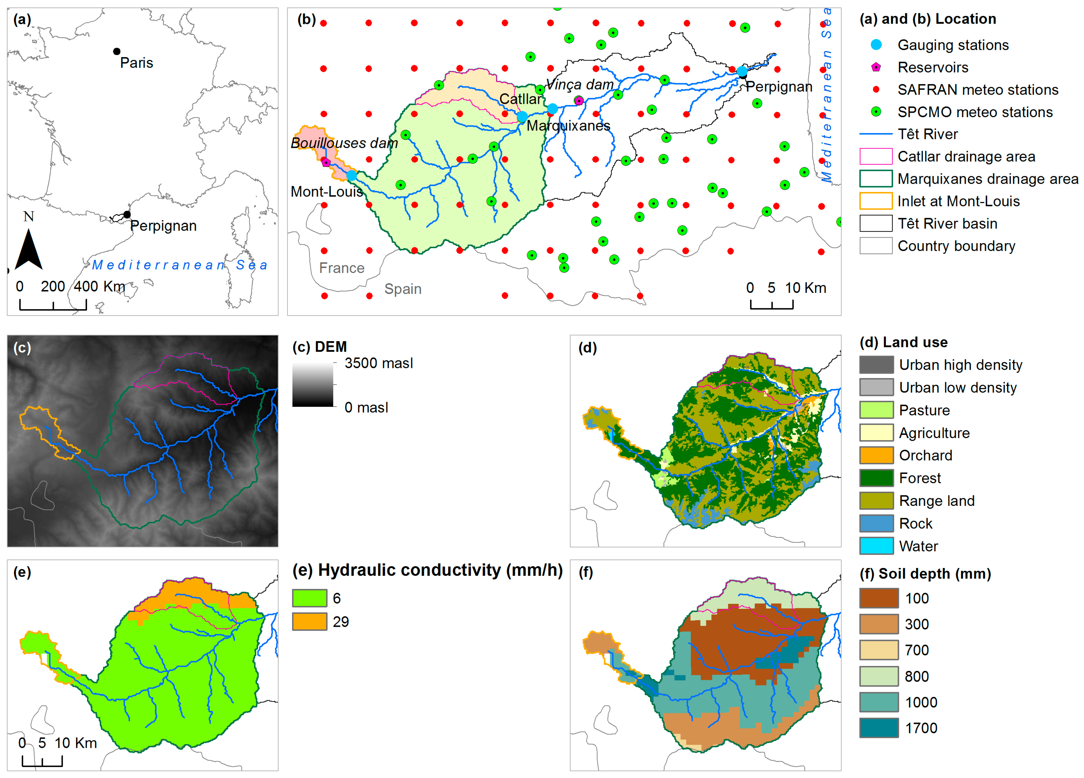
Figure 2.
Observed and SWAT simulated discharges (m3 s−1) with 95% confidence intervals (95PPU band) for both calibration (2009–2011) and validation (2012–2013) periods: (a) Simulated and observed discharge at Marquixanes at the daily time-step, using a minimum drainage area of 15 km2; (b) Simulated and observed discharge at Marquixanes at the hourly time-step, using a minimum drainage area of 15 km2; (c) Simulated and observed discharge at Marquixanes at the hourly time-step, using a minimum drainage area of 1 km2; (d) Simulated and observed discharge at Catllar at the hourly time-step, using a minimum drainage area of 15 km2. For better readability, the Y axes of the hourly figures were limited above the maximal observed hourly discharge, i.e., 161 m3 s−1 in Marquixanes and 50 m3 s−1 in Catllar, respectively.
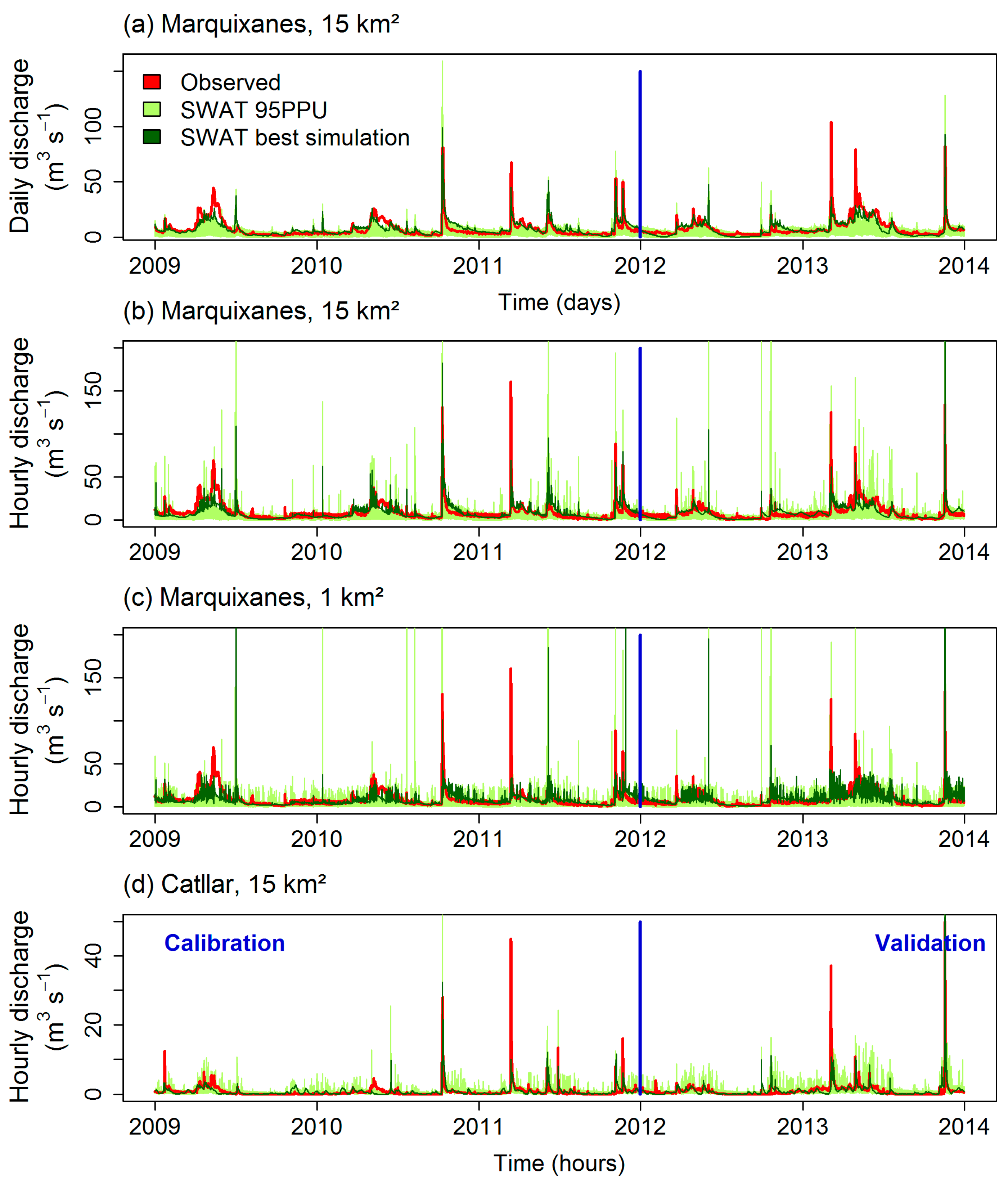
Figure 3.
Observed and SWAT-simulated flow duration curves (m3 s−1): (a) Simulated and observed discharge at Marquixanes at the daily time-step, using a minimum drainage area of 15 km2; (b) Simulated and observed discharge at Marquixanes at the hourly time-step, using a minimum drainage area of 15 km2; (c) Simulated and observed discharge at Marquixanes at the hourly time-step, using a minimum drainage area of 1 km2; (d) Simulated and observed discharge at Catllar at the hourly time-step, using a minimum drainage area of 15 km2.

Figure 4.
Distribution functions of behavioral simulations per event for (a) the CKSS (-) parameter and (b) the CZ (-) parameter.
Figure 4.
Distribution functions of behavioral simulations per event for (a) the CKSS (-) parameter and (b) the CZ (-) parameter.

Figure 5.
Sub-daily discharges (m3 s−1) simulated with both the SWAT (best simulation at hourly time-step) and MARINE (multi-event calibration at variable time-step) models and observed data for the six flash flood events that occurred in the Têt River basin (Marquixanes gauging station) from 2009 to 2013: (a) event from 7 October 7 to 27 October 2010; (b) event from 12 March to 20 March 2011; (c) event from 3 November to 15 November 2011; (d) event from 3 March to 15 March 2013; (e) event from 28 April to 7 May 2013; (f) event from 16 November to 23 November 2013. Maximal 95PPU upper limit is 806 m3 s−1.

Figure 6.
Soil water content (%) before and after the floods, and cumulative rainfall (mm) during the six major flood events in the Têt River basin from 2009 to 2013. Initial soil water content (before flood) was simulated with SWAT and SIM and final soil water content (after flood) was simulated with SWAT and MARINE. Cumulative rainfall was spatialized from rain gauge records with Thiessen polygons.
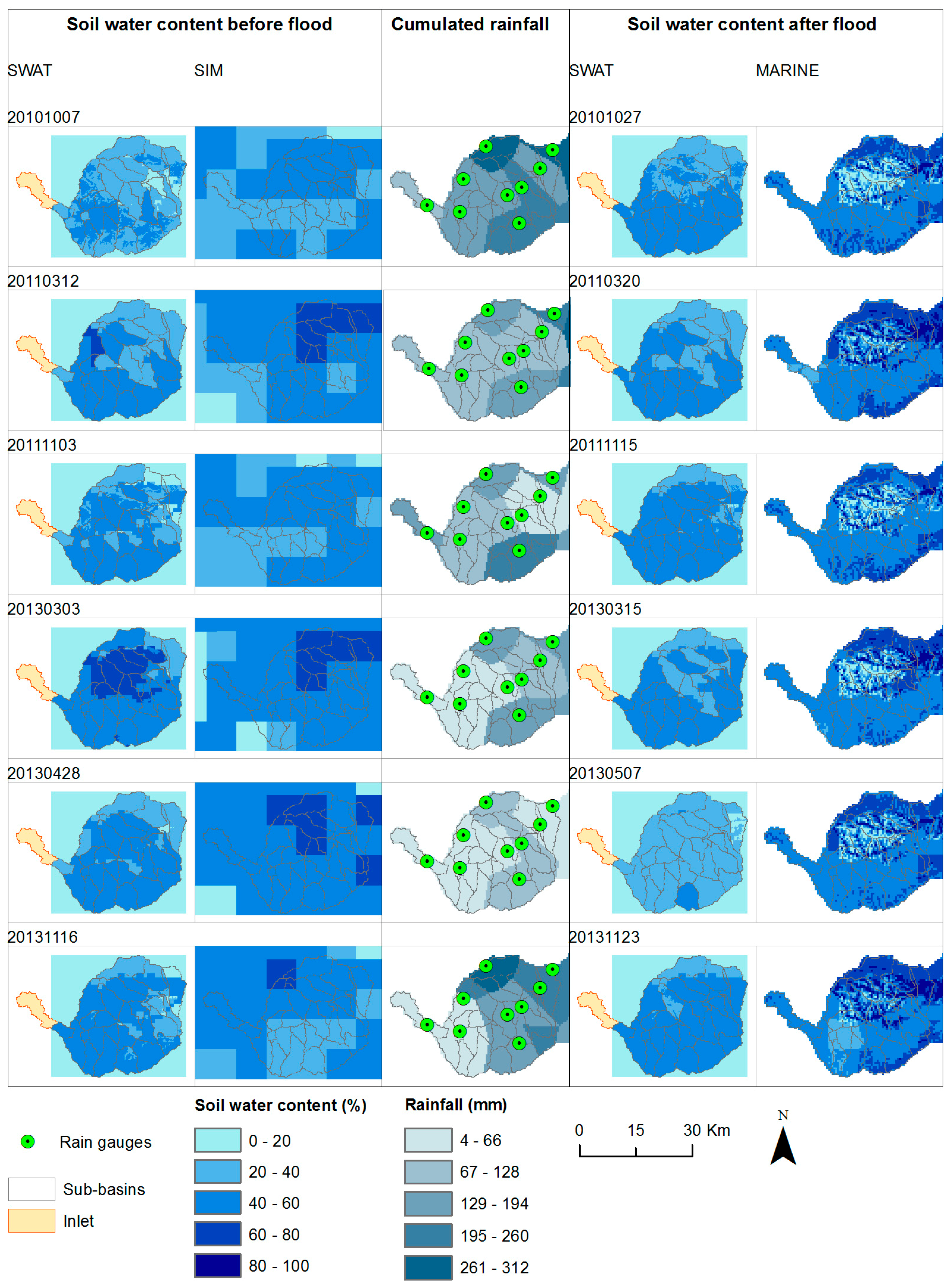

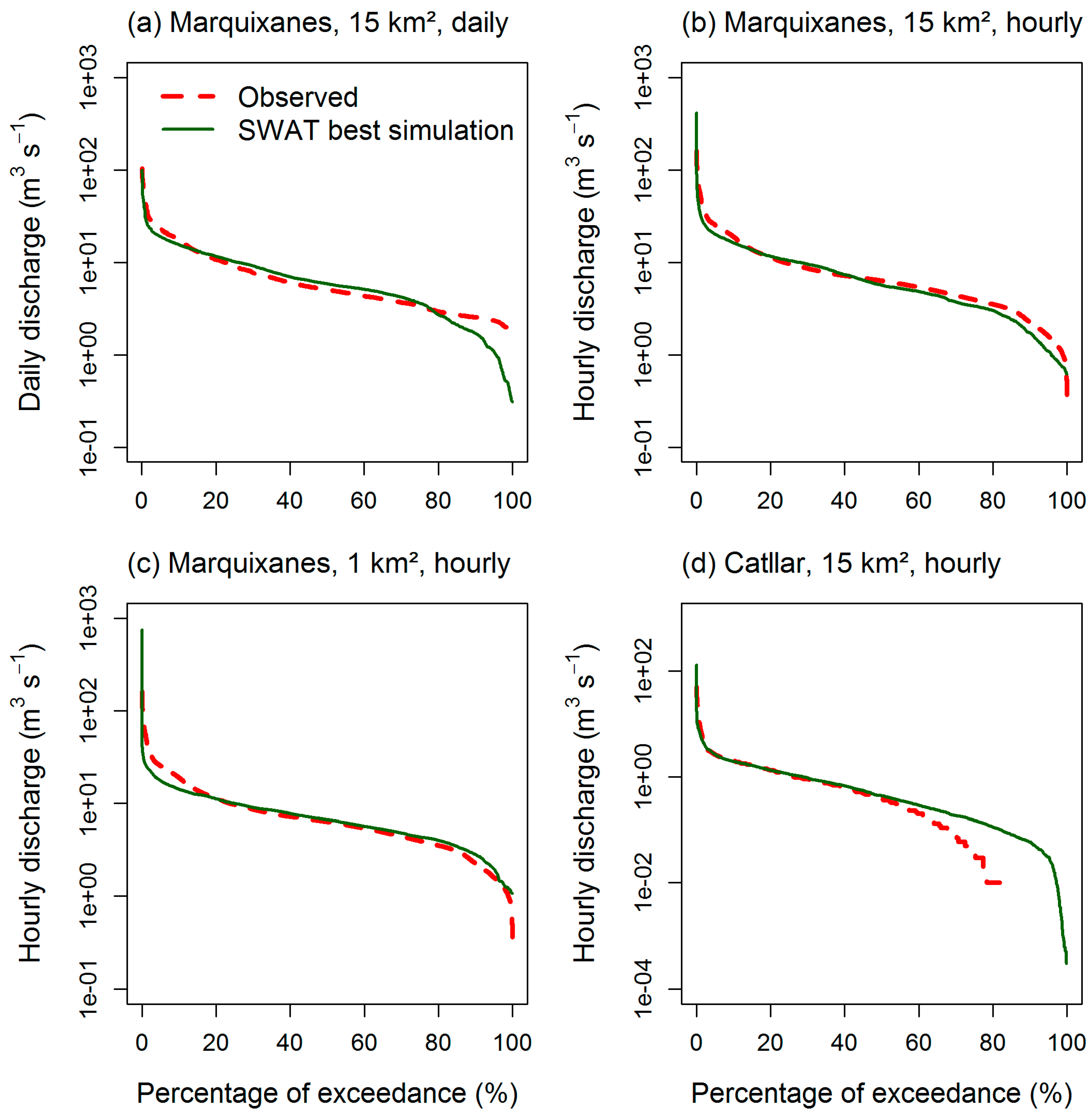
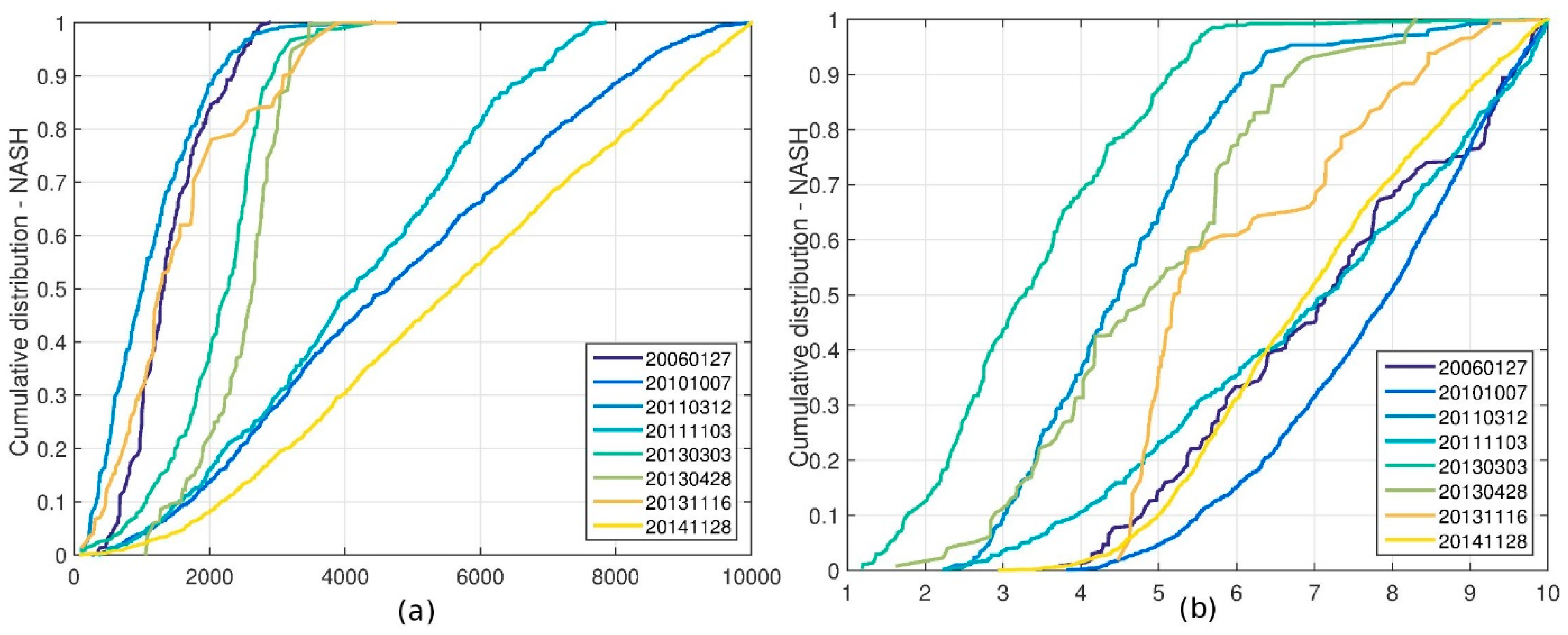
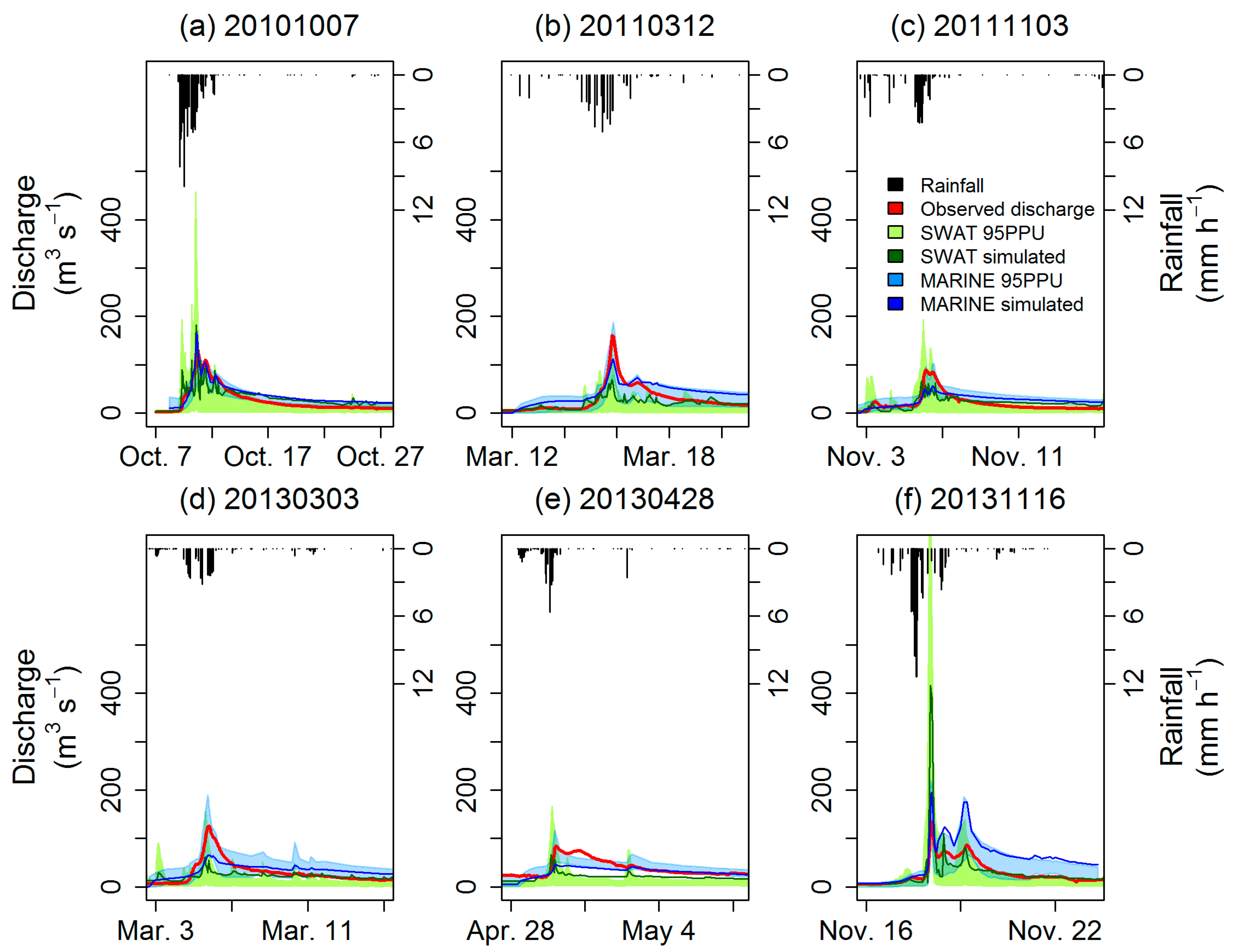
Table 1.
List of the flood events of interest for MARINE model calibration and validation from 2006 to 2014 at Marquixanes gauging station, and for comparison with the Soil and Water Assessment Tool (SWAT) at flood event-scale (hourly outputs, 15 km2 delineation scheme): peak discharge, time of peak and water exported volumes.
| Events | Dates of Flood Start and Flood End | Season | Observed | SWAT Simulated | MARINE Simulated | ||||||
|---|---|---|---|---|---|---|---|---|---|---|---|
| Peak Discharge (m3 s−1) | Time of Peak (UTC) | Volume (×106 m3) | Peak Discharge (m3 s−1) | Time of Peak (UTC) | Volume (×106 m3) | Peak Discharge (m3 s−1) | Time of Peak (UTC) | Volume (×106 m3) | |||
| 20060127 | 27/01/2006 14/02/2006 | Winter | 52 | 30/01 11:18 | 22.3 | - | - | - | 76 | 31/01 13:59 | 47.1 |
| 20101007 | 07/10/2010 27/10/2010 | Autumn | 123 | 11/10 15:59 | 38.3 | 182 | 11/10 14:00 | 54.1 | 165 | 11/10 14:35 | 62.1 |
| 20110312 | 12/03/2011 20/03/2011 | Spring | 159 | 15/03 21:16 | 21.5 | 70 | 15/03 21:00 | 15.5 | 112 | 15/03 21:16 | 31.6 |
| 20111103 | 03/11/2011 15/11/2011 | Autumn | 88 | 06/11 15:25 | 21.9 | 67 | 06/11 10:00 | 23.0 | 56 | 07/11 00:02 | 29.4 |
| 20130303 | 03/03/2013 15/03/2013 | Spring | 132 | 06/03 09:00 | 33.7 | 62 | 06/03 02:00 | 24.9 | 66 | 06/03 06:52 | 38.1 |
| 20130428 | 28/04/2013 07/05/2013 | Spring | 94 | 29/04 19:38 | 33.5 | 67 | 29/04 15:00 | 17.2 | 47 | 29/04 19:38 | 26.3 |
| 20131116 | 16/11/2013 23/11/2013 | Autumn | 165 | 18/11 01:15 | 20.4 | 416 | 18/11 01:00 | 19.3 | 196 | 18/11 01:45 | 36.0 |
| 20141128 | 28/11/2014 08/12/2014 | Autumn | 358 | 01/12 00:52 | 56.4 | - | - | - | 462 | 30/11 14:07 | 55.9 |
Table 2.
List of the parameters in SWAT changed for sensitivity analysis and for the calibration of discharge at an hourly time-step at the Marquixanes gauging station with a 15 km2 minimum drainage area watershed delineation: sensitivity ranks (1 being the most sensitive, 23 the least sensitive), initial ranges, and final calibrated ranges. Significantly sensitive parameters (p-values p < 0.001) are marked with * (H0: β = 0, reject if p < 0.001). In SWAT-CUP SUFI-2, two types of changes were used: “R” means the existing parameter value is multiplied by (1 + a given value); “V” means the existing parameter value is to be replaced by a given value.
| Parameter | Input File | Description | Type of Change | Sensitivity Rank | Initial Ranges | Calibrated Ranges | ||
|---|---|---|---|---|---|---|---|---|
| Min | Max | Min | Max | |||||
| CN2 | .mgt | Initial Soil Conservation Service (SCS) runoff curve number for moisture condition II (-) | R | 3 * | −0.1 | 0.1 | −0.1 | 0.1 |
| ALPHA_BF | .gw | Baseflow alpha factor (1/days) | V | 16 | 0.01 | 1 | 0.01 | 1 |
| GW_DELAY | .gw | Groundwater delay time (days) | V | 12 | 0 | 500 | 0 | 500 |
| GW_REVAP | .gw | Groundwater “revap“ coefficient (-) | V | 11 | 0.02 | 0.2 | 0.02 | 0.2 |
| GWQMN | .gw | Threshold depth of water in the shallow aquifer required for return flow to occur (mm H2O) | V | 10 | 0 | 5,000 | 0 | 5,000 |
| RCHRG_DP | .gw | Deep aquifer percolation fraction (-) | V | 4 * | 0.01 | 0.99 | 0.3 | 0.99 |
| REVAPMN | .gw | Threshold depth of water in the shallow aquifer for “revap” or percolation to the deep aquifer to occur (mm H2O) | V | 18 | 0 | 750 | 0 | 750 |
| CH_K2 | .rte | Effective hydraulic conductivity in main channel alluvium (mm/h) | V | 5 * | 0 | 127 | 30 | 127 |
| CH_N2 | .rte | Manning‘s “n“ value for the main channel (m−1/3 s) | V | 1 * | 0.014 | 0.15 | 0.045 | 0.15 |
| CH_K1 | .sub | Effective hydraulic conductivity in tributary channel alluvium (mm/h) | V | 7 | 0 | 127 | 0 | 127 |
| CH_N1 | .sub | Manning‘s “n“ value for the tributary channel (m−1/3 s) | V | 14 | 0.014 | 0.15 | 0.014 | 0.15 |
| TLAPS | .sub | Precipitation lapse rate (°C/km) | V | 6 | −8 | −4 | −8 | −4 |
| PLAPS | .sub | Temperature lapse rate (mm H2O/km) | V | 2 * | 0 | 500 | 0 | 200 |
| ESCO | .hru | Soil evaporation compensation factor (-) | V | 15 | 0.7 | 0.95 | 0.7 | 0.95 |
| EPCO | .hru | Plant uptake compensation factor (-) | V | 22 | 0.7 | 1 | 0.7 | 1 |
| LAT_TTIME | .hru | Lateral flow travel time (days) | V | 13 | 0 | 180 | 0 | 60 |
| CANMX | .hru | Maximum canopy storage (mm H2O) | V | 20 | 0 | 100 | 0 | 100 |
| OV_N | .hru | Manning‘s “n“ value for overland flow (m−1/3 s) | V | 8 | 0.01 | 0.6 | 0.01 | 0.6 |
| SOL_K | .sol | Saturated hydraulic conductivity (mm/h) | R | 19 | −0.1 | 0.1 | −0.1 | 0.1 |
| SOL_AWC | .sol | Available water capacity of the soil layer (mm H2O/mm soil) | R | 17 | −0.1 | 0.1 | −0.1 | 0.1 |
| SOL_BD | .sol | Moist bulk density (g/cm3) | R | 9 | −0.1 | 0.1 | −0.1 | 0.1 |
| SOL_CBN | .sol | Organic carbon content (%) | R | 23 | −0.1 | 0.1 | −0.1 | 0.1 |
| SURLAG | .bsn | Surface runoff lag coefficient (-) | V | 21 | 0.05 | 24 | 0.05 | 24 |
Table 3.
List of the catchment parameters and parameter ranges in MARINE. Sensitivity ranks are computed according to the maximum distance between the behavioral and non-behavioral distributions (1 is the most sensitive, 5 is the least sensitive). Fitted values are obtained with the best subset of calibration events.
| Parameter | Description | Initial Ranges | Units | Sensitivity Ranks | Fitted Values | |||||||||
|---|---|---|---|---|---|---|---|---|---|---|---|---|---|---|
| Min | Max | 20061027 | 20101007 | 20110312 | 20111103 | 20130303 | 20130428 | 20131116 | 20141128 | Average | ||||
| Correction coefficient of the soil thicknesses | 0.1 | 20 | - | 2 | 1 | 2 | 2 | 2 | 3 | 3 | 1 | 2.0 | 5.1 | |
| Correction coefficient of the hydraulic conductivities | 0.1 | 20 | - | 4 | 3 | 5 | 3 | 5 | 5 | 2 | 2 | 3.6 | 19.6 | |
| Correction coefficient of the soil lateral transmissivities | 100 | 10,000 | - | 1 | 2 | 1 | 1 | 1 | 1 | 1 | 3 | 1.4 | 1336.1 | |
| Manning’s roughness coefficient of the river bed | 1 | 30 | m−1/3 s | 3 | 4 | 3 | 4 | 4 | 2 | 4 | 4 | 3.5 | 9.2 | |
| Manning’s roughness coefficient of the flood plain | 1 | 20 | m−1/3 s | 5 | 5 | 4 | 5 | 3 | 4 | 5 | 5 | 4.5 | 15.4 | |
Table 4.
Goodness-of-fit indices for calibration (2009–2011) and validation (2012–2013) of the SWAT model at both the hourly and daily time-steps, for two minimum drainage area watershed delineations, and at two gauging stations. Numbers in bold highlight indices higher than the “satisfactory” thresholds suggested by Moriasi et al. [59] at daily (R2 and NS) and monthly (PBIAS) time-steps.
| Stations | Minimum Drainage Area | Time-Step | Simulation Period | p-Factor (-) | r-Factor (-) | R2 (-) | NS (-) | PBIAS (%) |
|---|---|---|---|---|---|---|---|---|
| Marquixanes | 15 km2 | Daily | Calibration | 0.86 | 1.05 | 0.65 | 0.65 | −4.7 |
| Validation | 0.85 | 0.98 | 0.66 | 0.64 | 13.5 | |||
| 15 km2 | Hourly | Calibration | 0.75 | 1 | 0.56 | 0.54 | 13.4 | |
| Validation | 0.84 | 1.05 | 0.49 | 0.45 | 7.6 | |||
| 1 km2 | Hourly | Calibration | 0.70 | 0.92 | 0.10 | −0.28 | 18.7 | |
| Validation | 0.83 | 1.05 | 0.28 | 0.21 | 0.6 | |||
| Catllar | 15 km2 | Hourly | Calibration | 0.53 | 0.79 | 0.48 | 0.46 | −34.3 |
| Validation | 0.63 | 0.83 | 0.35 | 0.32 | 17.2 |
Table 5.
Goodness-of-fit indices (Nash-Sutcliffe efficiencies) for the six flood events simulated with both the MARINE and the SWAT models at Marquixanes gauging station. Numbers in bold highlight Nash-Sutcliffe efficiencies higher than 0.5. Events marked with * are calibration events for MARINE.
Table 5.
Goodness-of-fit indices (Nash-Sutcliffe efficiencies) for the six flood events simulated with both the MARINE and the SWAT models at Marquixanes gauging station. Numbers in bold highlight Nash-Sutcliffe efficiencies higher than 0.5. Events marked with * are calibration events for MARINE.
| Model | 20061027 | 20101007 | 20110312 | 20111103 | 20130303 | 20130428 | 20131116 | 20141128 |
|---|---|---|---|---|---|---|---|---|
| MARINE | −0.55 | 0.80 * | 0.71 * | 0.60 * | 0.60 * | 0.38 | 0.39 | 0.64 |
| SWAT daily 15 km2 | - | 0.76 | 0.44 | 0.83 | 0.21 | −1.12 | 0.82 | - |
| SWAT hourly 15 km2 | - | 0.59 | 0.27 | 0.54 | 0.24 | −0.84 | −0.80 | - |
| SWAT hourly 1 km2 | - | −0.09 | −0.34 | 0.17 | −0.14 | −1.43 | −1.99 | - |
© 2017 by the authors. Licensee MDPI, Basel, Switzerland. This article is an open access article distributed under the terms and conditions of the Creative Commons Attribution (CC BY) license (http://creativecommons.org/licenses/by/4.0/).
Share and Cite
MDPI and ACS Style
Boithias, L.; Sauvage, S.; Lenica, A.; Roux, H.; Abbaspour, K.C.; Larnier, K.; Dartus, D.; Sánchez-Pérez, J.M. Simulating Flash Floods at Hourly Time-Step Using the SWAT Model. Water 2017, 9, 929. https://doi.org/10.3390/w9120929
AMA Style
Boithias L, Sauvage S, Lenica A, Roux H, Abbaspour KC, Larnier K, Dartus D, Sánchez-Pérez JM. Simulating Flash Floods at Hourly Time-Step Using the SWAT Model. Water. 2017; 9(12):929. https://doi.org/10.3390/w9120929
Chicago/Turabian StyleBoithias, Laurie, Sabine Sauvage, Anneli Lenica, Hélène Roux, Karim C. Abbaspour, Kévin Larnier, Denis Dartus, and José Miguel Sánchez-Pérez. 2017. "Simulating Flash Floods at Hourly Time-Step Using the SWAT Model" Water 9, no. 12: 929. https://doi.org/10.3390/w9120929
Note that from the first issue of 2016, this journal uses article numbers instead of page numbers. See further details here.