Performance Assessment of Spatial Interpolation of Precipitation for Hydrological Process Simulation in the Three Gorges Basin

Abstract

Accurate assessment of spatial and temporal precipitation is crucial for simulating hydrological processes in basins, but is challenging due to insufficient rain gauges. Our study aims to analyze different precipitation interpolation schemes and their performances in runoff simulation during light and heavy rain periods. In particular, combinations of different interpolation estimates are explored and their performances in runoff simulation are discussed. The study was carried out in the Pengxi River basin of the Three Gorges Basin. Precipitation data from 16 rain gauges were interpolated using the Thiessen Polygon (TP), Inverse Distance Weighted (IDW), and Co-Kriging (CK) methods. Results showed that streamflow predictions employing CK inputs demonstrated the best performance in the whole process, in terms of the Nash–Sutcliffe Coefficient (NSE), the coefficient of determination (R²), and the Root Mean Square Error (RMSE) indices. The TP, IDW, and CK methods showed good performance in the heavy rain period but poor performance in the light rain period compared with the default method (least sophisticated nearest neighbor technique) in Soil and Water Assessment Tool (SWAT). Furthermore, the correlation between the dynamic weight of one method and its performance during runoff simulation followed a parabolic function. The combination of CK and TP achieved a better performance in decreasing the largest and lowest absolute errors compared to any single method, but the IDW method outperformed all methods in terms of the median absolute error. However, it is clear from our findings that interpolation methods should be chosen depending on the amount of precipitation, adaptability of the method, and accuracy of the estimate in different rain periods.

1. Introduction

Precipitation is a major driving force of hydrological processes. Spatial precipitation patterns are consistently affected by topography and wind direction, which influence the estimation of the volume of storm runoff, peak runoff, and time-to-peak simulated by hydrological models [1]. In general, precipitation data are mainly sourced from precipitation gauges, re-analysis data or radar data [2]. Due to accessibility, this study focuses on precipitation data derived from rain gauges. However, obtaining accurate precipitation data in mountainous areas remains a challenge, mainly due to insufficient rain gauges [3,4].

Various convenient interpolation methods have been developed to simulate precipitation spatially [5,6]. The Thiessen Polygon (TP) and Inverse Distance Weighted (IDW) methods are the most popular deterministic methods, and both have been employed at varying spatial and temporal scales because of their simplicity [7]. Geostatistical methods, such as the Ordinary Kriging (OK), Co-Kriging (CK) and all the kriging variants, use the spatial correlation structure among observed data to estimate the spatial distribution of precipitation [7,8]. The precision of these methods is variable in different regions [9], but these methods give similar average areal precipitation values with the exception of extreme values [2]. When comparing different methods while considering sampling design, sample size, area of the region studied, and the associated results, kriging methods generally perform better than nongeostatistical methods [4,10]. Nevertheless, kriging methods usually overestimate the small values and underestimate large values [11].

The concept of combining different estimates in the same event has gained wide acceptance [12,13,14]. A number of different methods have been developed to merge radar and gauge rainfall estimates such as Mean Field Bias [14], Kalman Filter [15], and geostatistical approaches [16]. Combining precipitation estimates can exploit the strengths and minimize the weakness of each method, resulting in better predictions compared to the single method’s estimate [17]. Weighting schemes of geostatistical merging have been widely used [18,19]. The weights of radar and gauge rainfall estimates at each grid point are determined such that their linear combination minimizes the expected error variance of the estimate [20]. For example, Hasan et al. used a weighted combination approach to merge radar and spatially interpolated gauge rainfall estimates, and they concluded that the errors from the multiple estimates were correlated [21]. Furthermore, Woldemeskel et al. used a combination of thin plate smoothed splines and the IDW method to merge satellite and station data on a monthly time scale. They found that there was an improvement in rainfall estimation, particularly in regions with a sparse station network [22]. With the encouraging results reported by these preliminary studies, the present study applies the theory of weighting method to combining interpolation estimates. We therefore make the best use of available interpolation estimates and explore the influence of the combination of interpolation methods’ estimates on runoff simulation.

In general, to achieve the process-oriented simulation of hydrological processes, the variable basin inputs and runoff generation processes need to be adequately addressed by hydrological models [23,24,25,26,27]. The Soil and Water Assessment Tool (SWAT) is one of most commonly used hydrological models to predict the impact of weather data, land use, soil type, and slope on runoff simulation [28,29,30]. A considerable body of research demonstrated that the precipitation derived by interpolation methods for driving SWAT could enhance the performance of hydrological simulation [30,31,32,33]. For example, Masih et al. concluded that the Inverse Distance Elevation Weighted (IDEW) method outperformed the least sophisticated nearest neighbor (the default method used in SWAT), primarily, in small sub-catchments in the Karkheh basin in Iran [34].

However, there are only a few studies investigating interpolation uncertainties in different rain periods. The performance of process-based hydrological models is usually assessed through comparison between simulated and measured streamflow [29]. Although necessary, it is not sufficient to estimate the quality and realism of the modeling in the whole runoff process, because streamflow integrates different processes of the sub-basins including heavy and light rain periods [35]. Improvements to flow predictions depend on a wide range of factors such as rainfall event characteristics, runoff generation mechanisms, and applied models [36]. It is hard to assess whether the interpolation data improves the performance of modeling the runoff process during either a heavy or light rainfall period. Furthermore, large-scale processes are produced by integrating small-scale processes in space and time [27,37]; errors in estimated precipitation will result in a scale dilemma for runoff processes. Particularly in catchments with complex topography, the spatial distribution of precipitation is likely to be heterogeneous and the hydrological processes are more complex. This is the case in the Three Gorges Basin, where the world’s largest hydropower project is implemented—The Three Gorges Project. The project contributes significantly to socio-economic aspects in China, such as flood control, power generation, navigation, and water supply [38]. Due to the scarcity of accurate precipitation data, the development of water resource studies in this area is limited [33,39]. In a previous study carried out in the Daning River basin of the Three Gorges Basin, precipitation input was identified as a major source of error for runoff modeling [33].

In light of the issues discussed above, the main objectives of this study are: (i) to evaluate the performances of different interpolation schemes; (ii) to investigate the underlying differences in runoff process modeling with interpolation datasets during light and heavy rain events; and (iii) to analyze the performance of combining different estimates and the influence on runoff process modeling. The Pengxi River is one of the main tributaries on the north shore of the Three Gorges Basin. It is selected as a test basin because it has prominent heterogeneity and uncertainty of precipitation influenced by topography [39]. This paper is structured as follows: the description of study area, available data, interpolation methods, and the hydrological model are provided in Section 2. In Section 3, results of the precipitation estimates are demonstrated and different runoff processes are analyzed. Finally, conclusions are presented in Section 4.

2. Materials and Methods

2.1. Study Area

The Pengxi River is one of the main tributaries of the Yangtze River in the Three Gorges Basin (as shown in Figure 1), which is located in the Chongqing Municipality of China between the latitudes of 30.50° N–31.42° N and longitudes of 107.56° E–108.54° E. It extends over Yunyang County, Kai County and Wan County, with an altitude variation of 148–2549 m above mean sea level and an area of 5173 km². The length of the mainstream of Pengxi River is about 182 km. The basin is in a subtropical monsoon region, with relatively abundant rainfall and a humid climate. Average annual precipitation and temperature over the basin are 800–1500 mm and 18.5 °C, respectively. The average annual runoff is about 3.41 billion m³ [38]. Due to the serious extrusion of crustal movement and water erosion, the gully topography is very complex, with approximately 63% mountainous land and 31% hills.

2.2. Precipitation Data

Daily records for 16 selected rain gauges within or close to the Pengxi River basin (as shown in Figure 1) were provided by the Changjiang Water Resources Committee. The mean daily precipitation from 2009 to 2013 was 3.21 mm/d. The statistical information about the annual rainfall obtained from the daily rainfall records is displayed in

Table 1. Rain gauges, location, and statistics of mean annual precipitation from 2009 to 2013.

Gauge	Longitude (° E)	Latitude (° N)	Elevation (m)	Mean Annual Precipitation (mm)
Xinghua	108.63	31.01	510	1040.5
Guanmian	108.67	31.55	969	1780.1
Dajin	108.45	31.50	387	1250.2
Yanshui	108.65	31.45	1134	1516.3
Wenquan	108.55	31.33	269	1274.6
Wushan	107.95	30.95	262	1180.1
Nanya	108.08	31.08	385	1085.5
Linjiang	108.22	31.10	204	1098.4
Zhonghe	108.13	31.18	230	1071.8
Zhengba	108.30	31.35	401	1197.1
Hexing	107.82	30.73	418	1068.6
Qiaoting	108.08	30.80	591	1176.1
Yujia	107.95	30.82	332	1174.3
Nanmen	108.23	30.97	127	1053.8
Yanjinkou	107.55	30.60	444	1070.0
Gaolou	109.08	31.60	1858	1752.5

. It shows that the rain gauges with an elevation of over 900 m, such as Guanmian gauge, Yanshui gauge, and Gaoluo gauge, have higher mean annual precipitation.

2.3. Interpolation Schemes

The selection of interpolation methods in this paper was based on the popularity, in research papers, of different methods of precipitation interpolation. The three tested methods were Thiessen Polygons (TP), Inverse Distance Weighted (IDW), and Co-Kriging (CK). The literature review showed that these three methods were applied far more than other methods [2].

2.3.1. Thiessen Polygon

The TP method was developed by Thiessen [40]. According to the location of rain gauges, polygons are formed by the perpendicular bisectors of the lines joining nearby gauges. Thus, each polygon contains only one rain gauge, and the weights of the rain gauges are computed by their relative areas, which are estimated with the Thiessen polygon network. The average precipitation in each sub-basin is calculated in Equation (1). In this study, the mean precipitation generated in each sub-basin was incorporated into the hydrological simulation by creating a virtual rain gauge within the centroid of each sub-basin.

$$\stackrel{}{Z}(s_0)=\frac{Z(s_1)F_1+Z(s_2)F_2+\dots +Z(s_n)F_n}{F}={\displaystyle \sum _{i=1}^{n}Z(s_i)\frac{F_i}{F}}$$

(1)

where $\stackrel{}{Z}(s_0)$ is the average precipitation in the center of sub-basin; $Z(s_i)$ represents measured precipitation at the rain gauge $i$; $F_i$ is the area of Thiessen polygon associated with gauge $i$; $F$ is the area of the sub-basin.

2.3.2. Inverse Distance Weighting

The IDW method is based on the assumption that the value at an unsampled point can be approximated by the weighted average of observed values within a circular search neighborhood [41], the radius of which can be defined by the range of a fixed number of closest points. In our case, we adopted a localized IDW approach that only took the values of the rain gauges within a 50 km distance into account, based on a similar study by Wagner et al. [32]. The weights used for averaging are a decreasing function of the distance between the sampled and unsampled points. The weight ${\lambda }_i$ is proportional to the inverse distance between observations and $s_0$:

$$\stackrel{}{Z}(s_0)={\displaystyle \sum _{i=1}^N{\lambda }_{i}Z(s_i)}$$

(2)

where $\stackrel{}{Z}(s_0)$ is the predicted values at $s_0$; $N$ is the number of the sample points; ${\lambda }_i$ represents the weights, ${\displaystyle \sum _{i=1}^N{\lambda }_i=1}$;$Z(s_i)$ is the measured precipitation at $s_i$. The weight ${\lambda }_i$ is determined according to:

$${\lambda }_i=\frac{d_{i0}^{-p}}{{\displaystyle \sum _{i=1}^N{d}_{i0}^{-p}}}$$

(3)

where $d_{i0}$ is the distance between the prediction point $s_0$ and the known sample point $s_i$; the power exponent $p$ controls the decrease in weight with increasing distance. The higher exponents perform better closer to the coast line and lower exponents are preferred closer to the mountain crest [42]. In general, $p$ values are 1, 2 or 3 in mountainous areas [33]. In this paper, the value of $p$ was fixed as 2.

2.3.3. Co-Kriging

The CK method, based on the Ordinary Kriging (OK) method, is an interpolation method that introduces more than one relevant regionalized environmental factor affecting the interpolation results [8]. Theoretically, there is no essential difference between OK and CK methods. The CK method takes into account the combined effects of multiple variables that affect spatial information and can be derived from the OK method. When an environmental variable is incorporated in the study area, the information is introduced into CK as a second type of influencing factor. Some studies found it was beneficial to incorporate elevation into geostatistical methods for daily precipitation interpolation [7,43]. In this paper, the elevation data integrated as a correction factor was tested. The calculation equation is:

$$\stackrel{}{Z}(s_0)={\displaystyle \sum _{i=1}^n{\lambda }_i}Z(s_i)+\beta [y(s_i)-m_y+m_z]$$

(4)

where ${\displaystyle \sum _{i=1}^N{\lambda }_i=1}$, $\stackrel{}{Z}(s_0)$ is the predicted value at $s_0$; $Z(s_i)$ is the measured precipitation at $s_i$; $y(s_i)$ is the elevation of $s_i$; $n$ is the number of rain gauges; ${\lambda }_i$ and $\beta$ are the weight coefficients of CK; $m_y$ is the average elevation of all rain gauges and $m_z$ is the average precipitation of all rain gauges.

An experimental semi-variogram is adopted to assess the weight ${\lambda }_i$, which represents the spatial variation set against the distance, or separation, of input sample points. The empirical semi-variogram $y(h)$ is computed from the input data as follows:

$$y(h)=\frac{1}{2N}{\displaystyle \sum _{i=1}^N{\left[Z(x_i)-Z(x_i+h)\right]}^2}$$

(5)

where $N$ is the number of possible pairs of points; $Z(x_i)$ is the observed precipitation in the rain gauges, and $Z(x_i+h)$ is the value at a location moved by vector $h$. The experimental semi-variogram is a function of both distance and direction and is relatively easy to derive when the field has isotropy, which only depends on $h$. In this study, a local CK approach was applied taking only stations within a 50 km distance into account based on a similar study by Wagner et al. [32]. Next, a theoretical, continuous function needs to be fitted to the empirical semi-variogram. This function represents the spatial dependence structure of the data. Exponential, Gaussian, and spherical are the most commonly used variogram models for kriging applications in hydrology [44].

2.4. Combination of Interpolation Methods’ Estimates

A combined method is used to combine the interpolation methods’ estimates [17]. The basic equation for combining two methods’ estimates is:

$$\stackrel{}{Z}{(s_0)}_{\mathrm{COM},t}=w_{\mathrm{A}}\stackrel{}{Z}{(s_0)}_{\mathrm{A},t}+w_{\mathrm{B}}\stackrel{}{Z}{(s_0)}_{\mathrm{B},t}$$

(6)

where on a given day (t), $\stackrel{}{Z}{(s_0)}_{\mathrm{A},t}$ and $\stackrel{}{Z}{(s_0)}_{\mathrm{B},t}$ are the interpolated precipitation obtained from the two methods A and B. $w_{\mathrm{A}}$ and $w_{\mathrm{B}}$ are the weights applied to each method to provide a combined estimate $\stackrel{}{Z}{(s_0)}_{\mathrm{COM},t}$. In this paper, the weights $w_{\mathrm{A}}$ and $w_{\mathrm{B}}$ were tested as $w_{\mathrm{A}}+w_{\mathrm{B}}=1$.

2.5. Hydrologic Model

The SWAT is a semi-distributed hydrological model developed by the United States Department of Agriculture (USDA). Hydrologic processes simulated by SWAT include canopy storage, infiltration, redistribution, evapotranspiration, lateral subsurface flow, and surface flow [38]. In this study, the daily streamflow in the Pengxi River basin was simulated using SWAT. The Penman–Monteith and CN methods were applied to estimate evapotranspiration and runoff, respectively, and establish the water balance of each of the Hydrological Response Units (HRUs) [45,46,47,48].

In SWAT, the default precipitation interpolation method is a version of the least sophisticated nearest neighbor technique. The theory of this method is that the unknown values can be extracted by the nearby known points. The data from the rain gauge closest to the centroid of each sub-basin are selected as the sole input for that particular sub-basin. Then, the areal rainfall data are inputted directly into SWAT. The default method is best for qualitative data when other interpolation methods are not applicable. The disadvantages of only one sample point are considered and other nearby sample points are ignored for the estimated values, with no error estimate [8].

2.5.1. Model Setup

The available observed streamflow data from 2009 to 2013 in the Wenquan gauging station (as shown in Figure 1) were collected from the Changjiang Water Resources Committee. The Digital Elevation Model (DEM) map was obtained from the Data Center for Resource and Environmental Science, Chinese Academy of Science (RESDC), and was available at a grid size of 30 m × 30 m. Land use and land cover data were derived from GlobeLand30 and Landsat8. The soil map was created from a 1:1,000,000 digital map in China and available from the Institute of Soil Science, Chinese Academy of Science. Multi-year meteorological data including wind speed, temperature, and relative humidity data in five meteorological stations (Daxian, Wanyuan, Fengjie, Wanxian, and Liangpin stations, all of which are around the Pengxi River basin) were taken from the China Meteorological Data Sharing Service System [49]

2.5.2. Model Evaluation

The prediction uncertainty was quantified to analyze the model performance, by means of the Nash–Sutcliffe Coefficient (NSE), the coefficient of determination (R²), Root Mean Square Error (RMSE), Standard Deviation (SD), the Coefficient of Variation (CV) and Mean Absolute Error (MAE) which were defined in Equations (7)–(12).

$$E_{\mathrm{NS}}=1-\frac{{\displaystyle \sum _{i=1}^n{(x_{\mathrm{sim},i}-x_{\mathrm{mea},i})}^2}}{{\displaystyle \sum _{i=1}^n{(x_{\mathrm{mea},i}-\overline{x_{\mathrm{mea},i}})}^2}}$$

(7)

$${\mathrm{R}}^2={\left[\frac{{\displaystyle \sum _{i=1}^n(x_{\mathrm{mea},i}-\overline{x_{\mathrm{mea},i}})(x_{\mathrm{sim},i}-\overline{x_{\mathrm{sim},i}})}}{\sqrt{{\displaystyle \sum _{i=1}^n(x_{\mathrm{mea},i}-\overline{x_{\mathrm{mea},i}}){}^2{\displaystyle \sum _{i=1}^n(x_{\mathrm{sim},i}-\overline{x_{\mathrm{sim},i}}){}^2}}}}\right]}^2$$

(8)

$$\mathrm{RMSE}={\left\{\frac{1}{n}{\displaystyle \sum _{i=1}^n{(x_{\mathrm{sim},i}-x_{\mathrm{mea},\mathrm{i}})}^2}\right\}}^{0.5}$$

(9)

$$\mathrm{SD}=\sqrt{\frac{{\displaystyle \sum _{i=1}^n{(x_{\mathrm{sim}.i}-\overline{x_{\mathrm{sim}.i}})}^2}}{n-1}}$$

(10)

$$\mathrm{CV}=\frac{\mathrm{SD}}{\overline{x_{\mathrm{sim},i}}}$$

(11)

$$\mathrm{MAE}=\frac{{\displaystyle \sum _{i=1}^n\left|x_{\mathrm{sim},i}-x_{\mathrm{mea},i}\right|}}{n}$$

(12)

where $n$ was the number of simulation days; $x_{\mathrm{sim},i}$ and $x_{\mathrm{mea},i}$ were the SWAT daily simulated streamflow and measured streamflow (m³/s), respectively; $\overline{x_{\mathrm{sim},i}}$ and $\overline{x_{\mathrm{mea},i}}$ were the daily simulated average value and measured streamflow (m³/s), respectively.

3. Results and Discussion

3.1. Analysis of the Spatial Interpolation of Precipitation Distribution

In this paper, the SWAT was set up for the entire Pengxi River basin. Using watershed delineation and area threshold definition of each sub-basin in the SWAT, 25 sub-basins were derived (as shown in Figure 1). The precipitation in each centroid of the sub-basins, from 2009 to 2013, was calculated using three interpolation methods. The spatial rainfall variability in the sub-basins and the areal average annual rainfall input for each sub-basin are shown in

Table 2. The spatial rainfall variability in sub-basins and the areal rainfall input for each sub-basin.

Sub-Basin	Annual Average Precipitation (mm)				Mean (mm)	SD	CV
	Default	TP	IDW	CK
1	1379.4	978.4	960.0	974.6	1073.1	204.3	0.190
2	1379.4	1012.8	1084.2	1193.2	1167.4	159.6	0.137
3	999.3	978.4	960.0	974.6	978.1	16.2	0.017
4	1208.6	926.4	943.6	1037.4	1029.0	129.2	0.126
5	999.3	1012.8	1084.2	1193.2	1072.4	88.7	0.083
6	1208.6	1195.6	1000.3	1074.6	1119.8	99.9	0.089
7	1024.5	1195.6	1000.3	1074.6	1073.7	86.9	0.081
8	871.1	1012.8	1084.2	1193.2	1040.3	135.0	0.130
9	1024.5	856.6	979.6	1045.7	976.6	84.6	0.087
10	1024.5	1012.8	1084.2	1193.2	1078.7	82.5	0.077
11	834.5	898.1	959.6	1065.9	939.6	98.5	0.105
12	871.1	959.4	976.2	1105.4	978.0	96.6	0.099
13	871.1	857.0	898.7	901.4	882.0	21.6	0.024
14	835.7	959.4	976.2	1105.4	969.2	110.3	0.114
15	1024.5	946.1	921.4	968.3	965.1	43.9	0.046
16	1024.5	1208.5	1104.1	1299.6	1159.2	120.1	0.104
17	826.8	1245.5	1057.9	1284.1	1103.6	209.2	0.190
18	826.8	1012.8	1084.2	1193.2	1029.2	153.9	0.150
19	965.3	1245.5	1057.9	1284.1	1138.2	151.8	0.133
20	1024.5	1012.8	1084.2	1193.2	1078.7	82.5	0.077
21	944.8	1383.8	1016.8	1096.1	1110.4	192.4	0.173
22	806.9	1208.5	1104.1	1299.6	1104.8	214.0	0.194
23	944.8	1383.8	1016.8	1096.1	1110.4	192.4	0.173
24	872.1	867.7	1056.0	1173.7	992.4	149.3	0.151
25	959.3	1195.6	1000.3	1074.6	1057.4	103.7	0.098

Notes: TP is abbreviation of Thissen Polygen; IDW is abbreviation of Inverse Distance Weighting; CK is abbreviation of Co-Kriging; SD is abbreviation of standard deviation; CV is abbreviation of coefficient of variation.

. It indicates that CV values varied from 0.017 to 0.194 among sub-basins, with a range in SD of 16.2 to 214.0 mm. The greatest variability in a sub-basin level input was observed in sub-basin #22, in which the annual average rainfall (from low to high) was 806.9 mm for the default method, 1104.1 mm for the IDW method, 1208.5 mm for the TP method, and 1299.6 mm for the CK method. The smallest variation (a CV of 0.017) occurred in sub-basin #3, but there was still a 1.9% difference between the TP and IDW methods. This could be explained by the information presented in Figure 2, which illustrates high-intensity isolines in sub-basin #22, indicating a heterogeneous rainfall pattern, and low-intensity isolines in sub-basin #3 relating to a more homogeneous distribution of rainfall. The averaged SD and CV values for each sub-basin were 121.1 mm and 0.11, respectively. These interpolation methods result in considerable uncertainty of the spatial variability of rainfall, particularly at the sub-basin level, which is supported by similar studies [2,33].

Rainfall mapping of the results obtained by the four methods (Default, TP, IDW, and CK) in four typical months (March, June, September, and December) are shown in Figure 2. Valuable spatial and temporal visualizations of the rainfall distribution throughout the study region are provided. The changes in the spatial rainfall pattern from month to month are clearly depicted in all maps. The spatial trend in the rainfall distribution decreased from the northwest to the southeast during March, whereas an inverse trend is evident during June and September. The maximum precipitation (310 mm) is observed throughout the region during June to September, whereas the opposite trend is true during December. In addition, variations in the temporal rainfall pattern are clearly visible, with higher rainfall levels during June and September and lower rainfall levels in March and December.

Furthermore, important differences in the precipitation distribution among the four methods are also evident in the maps. As represented in Figure 2, the inefficient use of rain gauges in the default method resulted in jumping values of areal rainfall input in several sub-basins. For example, precipitation of over 90 mm was only depicted in the sub-basins #22 and #24 in March, while in sub-basins #4 and #6 the precipitation ranged from 60.1 to 70 mm. The TP method made use of the recorded data from rain gauges. The areal rainfall input of sub-watershed #4 was calculated by involving Guanmian and Yanshui gauges as well as Dajin and Wenquan gauges. A better description of the spatial rainfall distribution was obtained by weighting the nearby stations compared with the default method. The isolines obtained by the IDW, CK methods showed a homogeneously distributed spatial rainfall distribution from north to south. Spatial distributions of the CK rainfall estimates are represented by a continuous and smooth surface, which accurately represented the thermal and dynamic forcing mechanisms of the topography. In contrast, the map produced by the IDW method presents more isolines around the rain stations, for example, in the area between sub-basins #1 and #2, with lower precipitation in March, which is where the Guanmian gauge is located. This could be explained by the fact that the interpolated results using IDW were more significantly impacted by the nearby stations [33].

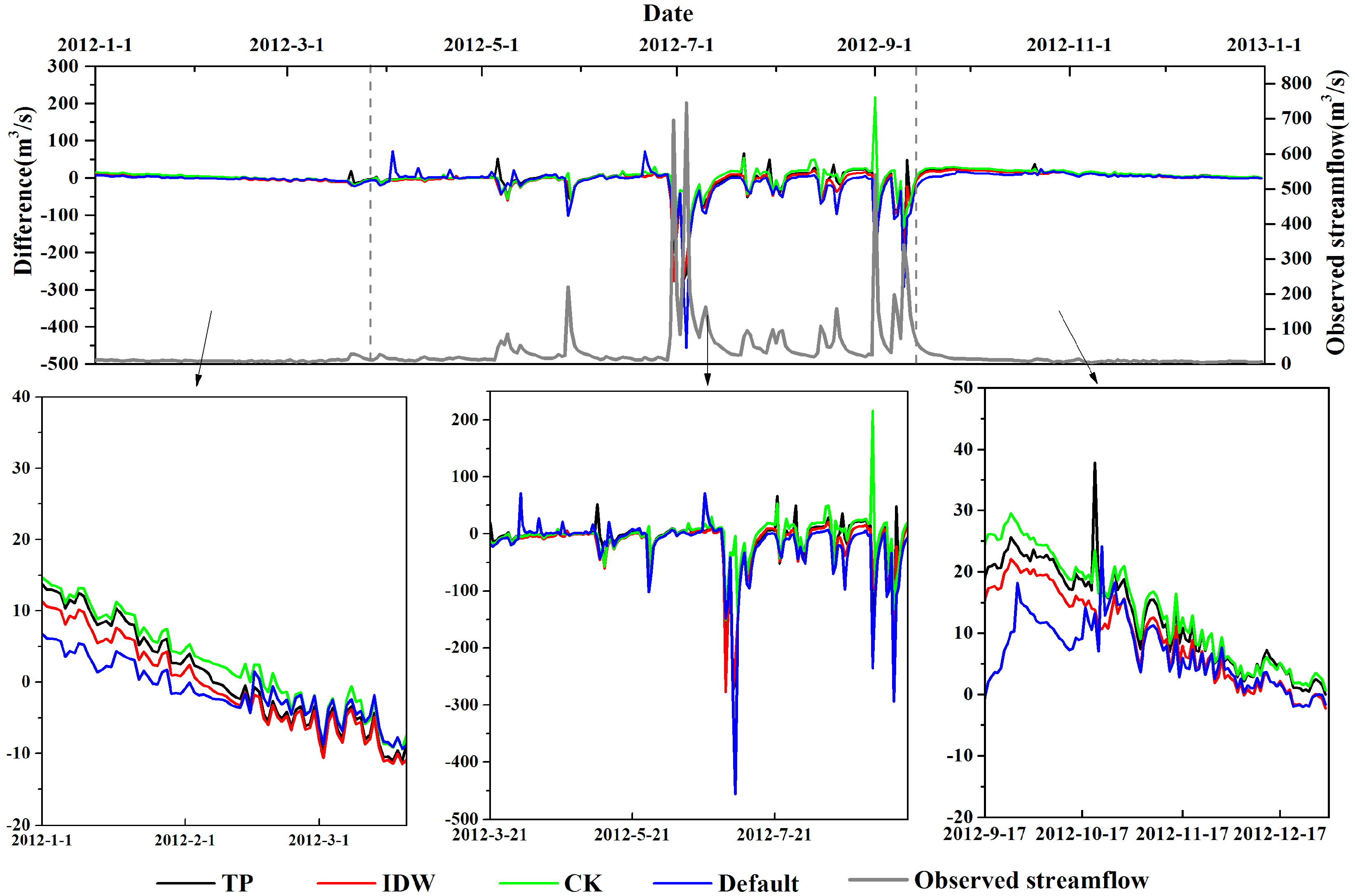
3.2. Analysis of Runoff Process by Spatial Interpolation of Precipitation

To illustrate the reliability of the SWAT performance, the observed precipitation data from 16 rain gauges were used as input data. Model calibration and validation were performed using the observed streamflow in the Wenquan gauging station. The model simulated a period of five years (2009–2013); data from the first year were considered as warm up time for the model, followed by model calibration using data from 2010 to 2011, whereas the remaining two years (2012–2013) of the dataset were employed for validating the model. The R² during the calibration and validation periods was 0.69 and 0.64, respectively. The NSE during calibration and validation periods was 0.77 and 0.73, respectively. More details about model calibration and validation and parameter optimization in the Pengxi River basin are available in the study by Shi et al. [34].

The performances of different interpolation methods were evaluated with the aforementioned calibrated parameters (described in Section 2.5.2). Results from the streamflow simulations in 2012 were shown in daily scales. The NSE, R² and RMSE indices for each dataset are displayed in

Table 3. Performance assessment of runoff modeling with different interpolated precipitation in 2012.

Method	NSE	R2	RMSE
Default	0.64	0.76	42.85
TP	0.75	0.81	35.29
IDW	0.76	0.83	35.06
CK	0.82	0.82	29.89

Notes: NSE is abbreviation of Nash-Sutcliffe coefficient; R² is abbreviation of coefficient of determination; RMSE is abbreviation of Root Mean Square Error.

. The best value for both NSE and R² is 1 (unit-less). For RMSE, a smaller value indicates better prediction. Results showed that the CK dataset performed very well on the daily scale simulation of discharge, and it had better NSE (0.82), R² (0.82), and RMSE (29.89) indices when compared to the runoff simulation using the default method (0.64, 0.76, and 42.85). The IDW method proved to be the second best dataset that was applied to the runoff simulation, with a NSE, R², and RMSE of 0.76, 0.83, and 35.06, respectively. The NSE, R², and RMSE indices of the TP method showed comparable values to the IDW method: 0.75, 0.81, and 35.29, respectively. These results demonstrated that the three interpolation schemes could improve runoff simulation in SWAT.

The default method produced a discrete and abrupt surface, while the other methods produced a smooth and gradual surface [8]. The smoothness depended on the criteria used in the selection of the weight values in relation to the distance between the point of interest and the sample points. The TP method typically showed reasonable performance for gauges, when the nearby gauge was representative of the estimated gauge [32]. The main reason why the IDW method outperformed the TP method depended on the differences in spatial precipitation distribution. The TP method produced a discrete and abrupt precipitation distribution, while the IDW method resulted in a smooth and gradual precipitation field. The smoothness relies on the criteria used in the selection of the weight values in relation to the distance between the point of interest and sample points [8]. This was in agreement with findings of Ruelland et al., who pointed out that IDW interpolation could significantly reduce error by adjusting the weighting factors used to reflect the relative influence of each station [50].

The precipitation dataset produced by the CK method had the best performance in terms of NSE, R², and RMSE, due to its estimated weights for donors found using a semi-variogram. On the other hand, the performance of the CK method could be ascribed to the very frequent application of an elevation correction factor in the case of the CK-based dataset. The CK method was found to be useful for regionalization of hydrological signatures [5,51]. It solved a problem of hydrological modeling in that the precipitation data were poorly resolved in space and could not capture heterogeneous orographic effects [52]. In particular, most available rain gauges in the Pengxi River basin were located at low elevations, which often led to an underestimation of precipitation input by other methods.

Figure 3 shows the differences between the simulated streamflow of different datasets and the observed streamflow in Wenquan gauging station of 2012. Large differences in flow were evident during the peaks. The same conclusion was obtained by Chen et al. that the hydrological response in the catchment associated with different interpolation methods could reflect a large difference [53]. Based on differences in the specific characteristics of streamflow, the year 2012 could be approximately divided into three periods. In the first period, 1 January to 20 March, there was no obvious improvement in the runoff process given by interpolation methods compared with the default method. However, interpolation methods performed well in the second period, from 21 March to 16 September, but poorly in the third period, from 17 September to 31 December.

For further analysis, the focus was set on the performances of interpolation methods during the three periods, the results of which are summarized in

Table 4. Performance assessment of runoff simulation with different interpolation schemes during three periods.

Method	First Period				Second Period				Third Period
	MAE	NSE	R2	RMSE	MAE	NSE	R2	RMSE	MAE	NSE	R2	RMSE
	(mm)			(mm)	(mm)			(mm)	(mm)			(mm)
Default	3.54	−4.36	0.14	4.2	26.88	0.59	0.75	60.6	6.92	−7.13	0.56	8.6
TP	6.19	−14.6	0.13	7.2	22.7	0.73	0.81	48.8	12.58	−24.05	0.59	14.8
IDW	5.62	−11.68	0.12	6.5	22.09	0.74	0.83	48.1	9.56	−14.85	0.72	11.8
CK	5.97	−14.57	0.1	7.2	20.12	0.82	0.83	40.5	13.78	−28.67	0.74	16.1

Note: MAE is abbreviation of Mean Absolute Error.

. In the first period, the values of MAE ranged from 3.54 to 6.19 mm/d during 1 January to 20 March. Results clearly demonstrated that the default method performed marginally better than the other methods in simulating streamflow, and the R² and RMSE were 0.14 and 4.2, respectively. The values of NSE in four methods were negative. In the second period, the CK method performed much better than other methods, with the lowest values of MAE and RMSE. The default method presented the weakest behavior during this period. In terms of R², the values were greater than 0.5 which were considered acceptable. The IDW method with an exponent of one performed similarly to the CK method, while the correlation in two points of the IDW method decreased almost linearly with increasing distance [32]. The CK method outperformed the IDW method in terms of NSE, with a value of 0.82. In the third period, the default method was slightly better than other methods with the MAE of 6.92 mm and RMSE of 8.6 mm. However, the values of NSE were also negative in the four methods.

Overall, the comparison of different methods in the three periods demonstrated that the CK method could reliably estimate precipitation-driven peaks in flow, as the peaks in precipitation and streamflow were closely matched in the time during 21 March to 16 September. However, in the first and third periods, an NSE less than zero occurred which indicated that the mean observed value was a better predictor than the simulated values [54]. In these two periods, the stimulated streamflow was underestimated or overestimated by the four methods. This situation could be explained by the fact that when extreme rainfalls occurred, i.e., higher or lower rainfall than the surrounding stations, the methods either overestimated or underestimated average rainfall because the estimation methods were affected by the surrounding rainfall stations [55]. In addition, we concluded that the response between precipitation and streamflow, as estimated by the SWAT, was not obvious in the light rain periods (dry periods) and prominent in heavy rain period (wet period). Several authors have previously addressed that SWAT’s predictive capabilities were less well-suited for drier conditions and consistently better during wet periods [56,57,58]. Different responses of the runoff to light and heavy rain could be attributed to the runoff response parameters in the SWAT [38]. One potential explanation for the difference performances is the model’s adjustment for curve number, which based upon antecedent moisture conditions does not accurately reflect the seasonal variations [57]. Another potential explanation is that the storage in the stream network riparian zone is not adequately represented in SWAT. Field research indicates that during dry periods, the water table in the riparian zone continues to be lowered by transpiration, which leads to water table depression results in storage [59].

3.3. Combination of Interpolation Methods’ Estimates for Runoff Process Simulation

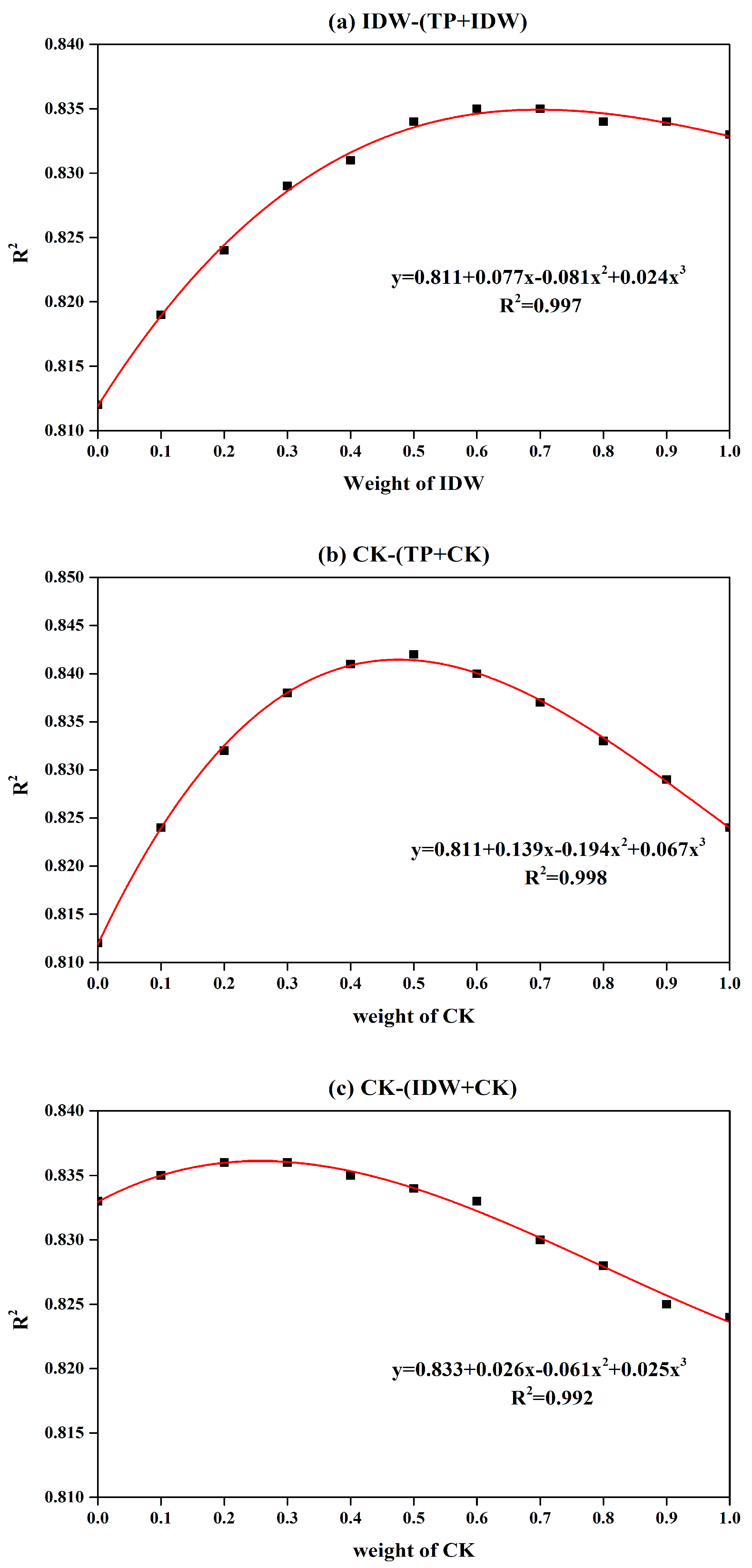
3.3.1. Combining Interpolation Methods’ Estimates

As noted previously, the relative influence of these various drivers of runoff could also be assessed by using multiple regression analysis. The correlation matrix, based on spatial interpolation of precipitation data in different methods, is presented in

Table 5. Correlation matrix between TP, IDW, and CK in interpolating precipitation in 2012.

Method	TP	IDW	CK
TP	1	0.89	0.83
IDW	—	1	0.96
CK	—	—	1

. It is evident that precipitation estimates from interpolation methods were significantly correlated with each other. The spatially interpolated precipitation estimate from the CK method showed a significant correlation with the estimate from the IDW method, and the R² was 0.96. By contrast, there were lower values of correlation between each of the CK and IDW methods and the TP method: 0.83 and 0.89, respectively. This implies that there was less variance of interpolated precipitation between the CK and IDW methods, considering the adaptable weights, compared with the TP method.

To account for the characteristics of interpolated precipitation among methods, further study was conducted to find out the model performance of combining interpolation methods’ estimates. Based on the algorithm in Hasan et al. [17] (as shown in Equation (6)), the results of three combination modes are shown in Figure 4. It can be seen that the relationship between the weight of one method and the performance of daily streamflow prediction accuracy, R², of the combined estimates followed a parabolic function. In the combination of IDW and TP methods’ estimates (Figure 4a), when the IDW method occupied a weight of 0.65, the peak of the fitting curve reached an R² of 0.835 and a NSE of 0.77. The CK method had a weight of 0.45 and the R² was 0.842 in the fitting curve for the combination of CK and TP methods’ estimates (Figure 4b), with an NSE of 0.83. As for the combination of IDW and CK methods’ estimates, the R² was 0.836 and NSE was 0.83 when the CK method had a weight of 0.25 (Figure 4c). Overall, the combination of the CK and TP methods’ estimates improved results compared to the best performance of a single method with an R² of 0.83 (see Table 3).

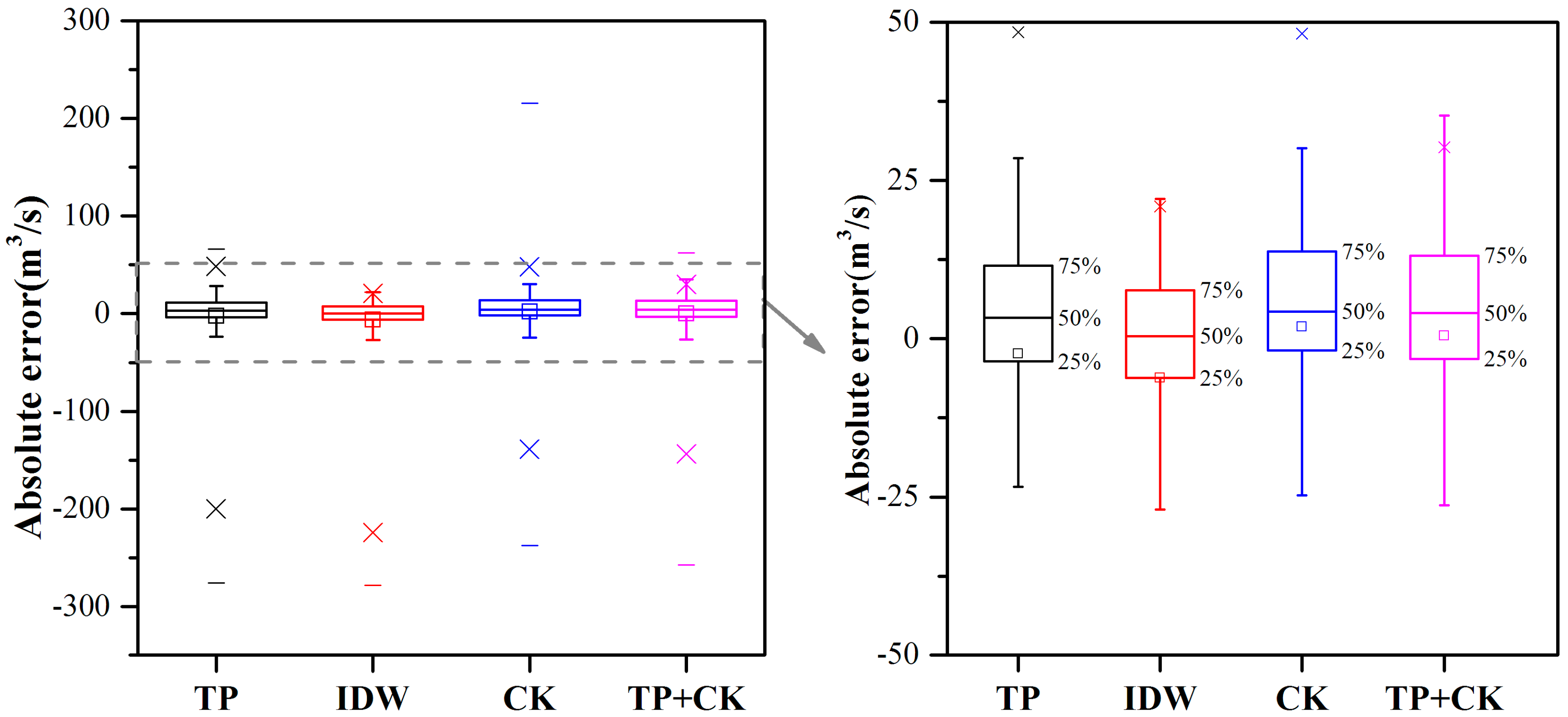
3.3.2. Performance Comparison

To further figure out the impact of the selection of the combination method on absolute error magnitude, the absolute error distributions of different methods are presented as box plots in Figure 5. The center represented the middle 50%, or 50th percentile, of the data set and was derived using the lower and upper quartile values. The median value was displayed inside the “box”. The maximum and minimum values were displayed with vertical lines (“whiskers”) connecting the points to the center box. As regards comparison among these methods, the results were quite variable, with the largest absolute error ranging from 22.08 m³/s (in the IDW method) to 215.6 m³/s (in the CK method) in the four methods.

In Figure 5, the largest and lowest absolute errors are derived from the CK and TP methods, respectively. The largest absolute error in the CK method was 215.6 m³/s on 1 September when the observed streamflow was 755.6 m³/s, and the lowest absolute error occurred on 3 July: −275.8 m³/s using the TP method when the observed streamflow was 321 m³/s. For the combination of CK and TP methods’ estimates, the absolute errors were decreased to 55 m³/s on 1 September and 257.48 m³/s on 3 July. On the right of Figure 5, it can be noted that the mean absolute error of 0.44 m³/s, found with the combination method, was the least, compared with the values of −2.36, −6.21, and 1.92 m³/s for the TP, IDW, and CK methods alone, respectively. However, the mean values were influenced by the outliers. The median values of the four methods were 3.4 m³/s, 0.4 m³/s, 4.5 m³/s, and 4.0 m³/s, respectively, which suggested that the IDW method outperformed other methods. It shows that combining estimates allowed minimization of the largest and lowest errors, resulting in better predictions compared with the single best method [8,17], but the median absolute error is still remarkable.

4. Conclusions

This paper detailed the results of the runoff process in SWAT with different interpolation precipitation datasets developed on the Three Gorges Basin. The performances of spatial interpolation of precipitation using the TP, IDW, and CK methods were evaluated, and the causes of the differences in model performance between light and heavy rain were revealed. Furthermore, combinations of the different interpolation estimates and the influence this has on runoff process simulation were analyzed. The major results were summarized as follows:

(i) Three interpolation methods were noticeably better than the default approach at streamflow modeling during the whole process. The CK methods showed the best performance in terms of NSE, R², and RMSE indexes.

(ii) Compared with the default method in SWAT, the TP, IDW, and CK methods were less reliable in accurately predicting low flows in light rain periods (dry periods) but performed better in heavy rain periods (wet periods). In the dry periods, the three methods obviously reflected a trend of underestimation or overestimation of precipitation because the estimation methods were affected by the surrounding rainfall stations. In addition, the poor performance in the dry periods also demonstrated that SWAT’s predictive capabilities were less well-suited in drier conditions for poor precipitation-runoff response in the SWAT.

(iii) Three merging interpolated estimates were examined; they differed in the correlation between the dynamic weight of one method and the performance of runoff simulation. The combination of TP and CK methods’ estimates performed best in accurately predicting streamflow in terms of R², for minimizing the largest and lowest errors. However, by taking the median absolute error of streamflow into account, it was clear from our findings that the IDW method produced the least absolute errors compared to other methods including the combined estimates.

Overall, our study underlines that interpolation methods should be embedded in SWAT during the heavy rain period to capture rainfall characteristics for runoff process simulation. Furthermore, through the analysis of simulation results, a combination of interpolation estimates yielded no obvious improvement in hydrological modeling in terms of absolute errors. The spatial interpolation of precipitation for runoff process simulation needs to be further explored in the future. The results further elucidate the effect of spatial interpolation of precipitation on predicting runoff processes.

References

1. Caracciolo, D.; Arnone, E.; Noto, L.V. Influence of spatial precipitation sampling on hydrological response at the catchment scale. J. Hydrol. Eng. 2014, 19, 544–553. [Google Scholar] [CrossRef]
2. Szcześniak, M.; Piniewski, M. Improvement of hydrological simulations by applying daily precipitation interpolation schemes in meso-scale catchments. Water 2015, 7, 747–779. [Google Scholar] [CrossRef]
3. Cristiano, E.; ten Veldhius, M.-C.; van de Giesen, N. Spatial and temporal variability of rainfall and their effects on hydrological response in urban areas—A review. Hydrol. Earth Syst. Sci. Discuss. 2017, 21, 3859–3878. [Google Scholar] [CrossRef]
4. Li, J.; Heap, A.D. A review of comparative studies of spatial interpolation methods in environmental sciences: Performance and impact factors. Ecol. Inform. 2011, 6, 228–241. [Google Scholar] [CrossRef]
5. Xu, W.; Zou, Y.; Zhang, G.; Linderman, M. A comparison among spatial interpolation techniques for daily rainfall data in Sichuan province, China. Int. J. Climatol. 2015, 35, 2898–2907. [Google Scholar] [CrossRef]
6. Bayat, B.; Zahraie, B.; Taghavi, F.; Nasseri, M. Evaluation of spatial and spatiotemporal estimation methods in simulation of precipitation variability patterns. Theor. Appl. Climatol. 2012, 113, 429–444. [Google Scholar] [CrossRef]
7. Ly, S.; Charles, C.; Degré, A. Different methods for spatial interpolation of rainfall data for operational hydrology and hydrological modeling at watershed scale. A review. Biotechnol. Agron. Soc. Environ. 2013, 17, 392–406. [Google Scholar]
8. Li, J.; Heap, A.D. Spatial interpolation methods applied in the environmental sciences: A review. Environ. Model. Softw. 2014, 53, 173–189. [Google Scholar] [CrossRef]
9. Zareian, M.J.; Eslamian, S.; Safavi, H.R. A modified regionalization weighting approach for climate change impact assessment at watershed scale. Theor. Appl. Climatol. 2014, 122, 497–516. [Google Scholar] [CrossRef]
10. Borges, P.D.A.; Franke, J.; da Anunciação, Y.M.T.; Weiss, H.; Bernhofer, C. Comparison of spatial interpolation methods for the estimation of precipitation distribution in distrito Federal, Brazil. Theor. Appl. Climatol. 2015, 123, 335–348. [Google Scholar] [CrossRef]
11. Yamamoto, J.K. Correcting the smoothing effect of ordinary kriging estimates. Math. Geol. 2005, 37, 69–94. [Google Scholar] [CrossRef]
12. Sinclair, S.; Pegram, G. Combining radar and rain gauge rainfall estimates using conditional merging. Atmos. Sci. Lett. 2005, 6, 19–22. [Google Scholar] [CrossRef]
13. Wardhana, A.; Pawitan, H.; Dasanto, B.D. Application of hourly radar-gauge merging method for quantitative precipitation estimates. IOP Conf. Ser. Earth Environ. Sci. 2017, 58, 012033. [Google Scholar] [CrossRef]
14. Berndt, C.; Rabiei, E.; Haberlandt, U. Geostatistical merging of rain gauge and radar data for high temporal resolutions and various station density scenarios. J. Hydrol. 2014, 508, 88–101. [Google Scholar] [CrossRef]
15. Chowdhury, S.; Sharma, A. Global sea surface temperature forecasts using a pairwise dynamic combination approach. J. Clim. 2011, 24, 1869–1877. [Google Scholar] [CrossRef]
16. Goudenhoofdt, E.; Delobbe, L. Evaluation of radar-gauge merging methods for quantitative precipitation estimates. Hydrol. Earth Syst. Sci. 2008, 13, 195–203. [Google Scholar] [CrossRef]
17. Hasan, M.M.; Sharma, A.; Johnson, F.; Mariethoz, G.; Seed, A. Merging radar and in situ rainfall measurements: An assessment of different combination algorithms. Water Resour. Res. 2016, 52, 8384–8398. [Google Scholar] [CrossRef]
18. Robertson, A.W.; Lall, U.; Zebiak, S.E.; Goddard, L. Improved combination of multiple atmospheric gcm ensembles for seasonal prediction. Mon. Weather Rev. 2003, 132, 2732–2744. [Google Scholar] [CrossRef]
19. Krishnamurti, T.N.; Kishtawal, C.M.; Zhang, Z.; Larow, T.; Bachiochi, D.; Williford, E.; Gadgil, S.; Surendran, S. Multimodel ensemble forecasts for weather and seasonal climate. J. Clim. 2000, 13, 4196–4216. [Google Scholar] [CrossRef]
20. S̆alek, M. The radar and raingauge merge precipitation estimate of daily rainfall—First results in the Czech Republic. Phys. Chem. Earth Part B Hydrol. Oceans Atmos. 2000, 25, 977–979. [Google Scholar] [CrossRef]
21. Hasan, M.M.; Sharma, A.; Mariethoz, G.; Johnson, F.; Seed, A. Improving radar rainfall estimation by merging point rainfall measurements within a model combination framework. Adv. Water Resour. 2016, 97, 205–218. [Google Scholar] [CrossRef]
22. Woldemeskel, F.M.; Sivakumar, B.; Sharma, A. Merging gauge and satellite rainfall with specification of associated uncertainty across australia. J. Hydrol. 2013, 499, 167–176. [Google Scholar] [CrossRef]
23. Guan, K.; Thompson, S.E.; Harman, C.J.; Basu, N.B.; Rao, P.S.C.; Sivapalan, M.; Packman, A.I.; Kalita, P.K. Spatiotemporal scaling of hydrological and agrochemical export dynamics in a tile-drained midwestern watershed. Water Resour. Res. 2011, 47, W00J02. [Google Scholar] [CrossRef]
24. Ye, X.; Zhang, Q.; Viney, N.R. The effect of soil data resolution on hydrological processes modelling in a large humid watershed. Hydrol. Process. 2011, 25, 130–140. [Google Scholar] [CrossRef]
25. Clark, M.P.; Nijssen, B.; Lundquist, J.D.; Kavetski, D.; Rupp, D.E.; Woods, R.A.; Freer, J.E.; Gutmann, E.D.; Wood, A.W.; Gochis, D.J.; et al. A unified approach for process-based hydrologic modeling: 2. Model implementation and case studies. Water Resour. Res. 2015, 51, 2515–2542. [Google Scholar] [CrossRef]
26. Wang, J.; Hassett, J.M.; Endreny, T.A. An object oriented approach to the description and simulation of watershed scale hydrologic processes. Comput. Geosci. 2005, 31, 425–435. [Google Scholar] [CrossRef]
27. Uhlenbrook, S.; Roser, S.; Tilch, N. Hydrological process representation at the meso-scale: The potential of a distributed, conceptual catchment model. J. Hydrol. 2004, 291, 278–296. [Google Scholar] [CrossRef]
28. Gitau, M.W.; Chaubey, I. Regionalization of swat model parameters for use in ungauged watersheds. Water 2010, 2, 849–871. [Google Scholar] [CrossRef]
29. Chaponnière, A.; Boulet, G.; Chehbouni, A.; Aresmouk, M. Understanding hydrological processes with scarce data in a mountain environment. Hydrol. Process. 2008, 22, 1908–1921. [Google Scholar] [CrossRef] [Green Version]
30. Galván, L.; Olías, M.; Izquierdo, T.; Cerón, J.C.; Fernández de Villarán, R. Rainfall estimation in swat: An alternative method to simulate orographic precipitation. J. Hydrol. 2014, 509, 257–265. [Google Scholar] [CrossRef]
31. Vu, M.T.; Raghavan, S.V.; Liong, S.Y. Swat use of gridded observations for simulating runoff—A Vietnam River basin study. Hydrol. Earth Syst. Sci. 2012, 16, 2801–2811. [Google Scholar] [CrossRef] [Green Version]
32. Wagner, P.D.; Fiener, P.; Wilken, F.; Kumar, S.; Schneider, K. Comparison and evaluation of spatial interpolation schemes for daily rainfall in data scarce regions. J. Hydrol. 2012, 464–465, 388–400. [Google Scholar] [CrossRef]
33. Shen, Z.; Chen, L.; Liao, Q.; Liu, R.; Hong, Q. Impact of spatial rainfall variability on hydrology and nonpoint source pollution modeling. J. Hydrol. 2012, 472–473, 205–215. [Google Scholar] [CrossRef]
34. Masih, I.; Maskey, S.; Uhlenbrook, S.; Smakhtin, V. Assessing the impact of areal precipitation input on streamflow simulations using the swat model1. JAWRA J. Am. Water Resour. Assoc. 2011, 47, 179–195. [Google Scholar] [CrossRef]
35. Di Lazzaro, M.; Zarlenga, A.; Volpi, E. Hydrological effects of within-catchment heterogeneity of drainage density. Adv. Water Resour. 2015, 76, 157–167. [Google Scholar] [CrossRef]
36. Tetzlaff, D.; Uhlenbrook, U. Effects of spatial variability of precipitation for process-orientated hydrological modelling: Results from two nested catchments. Hydrol. Earth Syst. Sci. Discuss. 2005, 2, 119–154. [Google Scholar] [CrossRef]
37. Yu, Z.; Lu, Q.; Zhu, J.; Yang, C.; Ju, Q.; Yang, T.; Chen, X.; Sudicky, E.A. Spatial and temporal scale effect in simulating hydrologic processes in a watershed. J. Hydrol. Eng. 2014, 19, 99–107. [Google Scholar] [CrossRef]
38. Shi, Y.; Xu, G.; Wang, Y.; Engel, B.A.; Peng, H.; Zhang, W.; Cheng, M.; Dai, M. Modelling hydrology and water quality processes in the pengxi river basin of the three gorges reservoir using the soil and water assessment tool. Agric. Water Manag. 2017, 182, 24–38. [Google Scholar] [CrossRef]
39. Hui, D.; Yang, Y.; Wang, G.; Wang, L.; Yu, J.; Xu, Z. Evaluation of gridded precipitation data for driving swat model in area upstream of three gorges reservoir. PLoS ONE 2014, 9, e112725. [Google Scholar]
40. Thiessen, A.H. Precipitation averages for large areas. Mon. Weather Rev. 1911, 39, 1082. [Google Scholar] [CrossRef]
41. Mair, A.; Fares, A. Comparison of rainfall interpolation methods in a mountainous region of a tropical island. J. Hydrol. Eng. 2011, 16, 371–383. [Google Scholar] [CrossRef]
42. Kurtzman, D.; Navon, S.; Morin, E. Improving interpolation of daily precipitation for hydrologic modelling: Spatial patterns of preferred interpolators. Hydrol. Process. 2010, 23, 3281–3291. [Google Scholar] [CrossRef]
43. Jacquin, A.P.; Soto-Sandoval, J.C. Interpolation of monthly precipitation amounts in mountainous catchments with sparse precipitation networks. Chil. J. Agric. Res. 2013, 73, 406–413. [Google Scholar] [CrossRef]
44. Adhikary, S.K.; Yilmaz, A.G.; Muttil, N. Optimal design of rain gauge network in the middle yarra river catchment, australia. Hydrol. Process. 2015, 29, 2582–2599. [Google Scholar] [CrossRef]
45. Seo, M.; Yen, H.; Kim, M.-K.; Jeong, J. Transferability of swat models between SWAT2009 and SWAT2012. J. Environ. Qual. 2014, 43, 869–880. [Google Scholar] [CrossRef] [PubMed]
46. Vazquez-Amabile, G.G.; Engel, B.A. Fitting of time series models to forecast streamflow and groundwater using simulated data from swat. J. Hydrol. Eng. 2008, 13, 554–562. [Google Scholar] [CrossRef]
47. Humphrey, C.P.; Jernigan, J.; Iverson, G.; Serozi, B.; O’Driscoll, M.; Pradhan, S.; Bean, E. Field evaluation of nitrogen treatment by conventional and single-pass sand filter onsite wastewater systems in the north carolina piedmont. Water Air Soil Pollut. 2016, 227, 1–17. [Google Scholar] [CrossRef]
48. Feng, Q.; Chaubey, I.; Engel, B.; Cibin, R.; Sudheer, K.P.; Volenec, J. Marginal land suitability for switchgrass, Miscanthus and hybrid poplar in the Upper Mississippi River Basin (UMRB). Environ. Model. Softw. 2017, 93, 356–365. [Google Scholar] [CrossRef]
49. China Meteorological Data Sharing Service System. Available online: http://data.cma.cn (accessed on 12 September 2016).
50. Ruelland, D.; Ardoin-Bardin, S.; Billen, G.; Servat, E. Sensitivity of a lumped and semi-distributed hydrological model to several methods of rainfall interpolation on a large basin in West Africa. J. Hydrol. 2008, 361, 96–117. [Google Scholar] [CrossRef]
51. Adhikary, S.K.; Muttil, N.; Yilmaz, A.G. Cokriging for enhanced spatial interpolation of rainfall in two Australian catchments. Hydrol. Process. 2017, 31, 2143–2161. [Google Scholar] [CrossRef]
52. Fatichi, S.; Vivoni, E.R.; Ogden, F.L.; Ivanov, V.Y.; Mirus, B.; Gochis, D.; Downer, C.W.; Camporese, M.; Davison, J.H.; Ebel, B.; et al. An overview of current applications, challenges, and future trends in distributed process-based models in hydrology. J. Hydrol. 2016, 537, 45–60. [Google Scholar] [CrossRef]
53. Chen, T.; Ren, L.; Yuan, F.; Yang, X.; Jiang, S.; Tang, T.; Liu, Y.; Zhao, C.; Zhang, L. Comparison of spatial interpolation schemes for rainfall data and application in hydrological modeling. Water 2017, 9, 342. [Google Scholar] [CrossRef]
54. Moriasi, D.N.; Arnold, J.G.; Van Liew, M.W.; Bingner, R.L.; Harmel, R.D.; Veith, T.L. Model evaluation guidelines for systematic quantification of accuracy in watershed simulations. Trans. ASABE 2007, 50, 885–900. [Google Scholar] [CrossRef]
55. Abo-Monasar, A.; Al-Zahrani, M.A. Estimation of rainfall distribution for the southwestern region of saudi arabia. Hydrol. Sci. J. 2014, 59, 420–431. [Google Scholar] [CrossRef]
56. Tobin, K.J.; Bennett, M.E. Temporal analysis of Soil and Water Assessment Tool (SWAT) performance based on remotely sensed precipitation products. Hydrol. Process. 2013, 27, 505–514. [Google Scholar] [CrossRef]
57. Feyereisen, G.W.; Strickland, T.C.; Bosch, D.D.; Sullivan, D.G. Evaluation of swat manual calibration and input parameter sensitivity in the little river watershed. Trans. ASABE 2007, 50, 843–855. [Google Scholar] [CrossRef]
58. Van Liew, M.W.; Arnold, J.G.; Bosch, D.D. Problems and potential of autocalibrating a hydrologic model. Trans. ASAE 2005, 48, 1025–1040. [Google Scholar] [CrossRef]
59. Shirmohammadi, A.; Sheridan, J.M.; Asmussen, L.E. Hydrology of alluvial stream channels in southern coastal plain watersheds. Trans. ASAE 1986, 29, 0135–0142. [Google Scholar] [CrossRef]
Figure 1. Location of gauging station (green solid circle), rain gauges (red solid triangle), and topography in the Pengxi River basin.
Water 09 00838 g001
Figure 2. Mean monthly rainfall maps by TP (the first row), IDW (the second row) and CK (the third row) in March, June, September and December from 2009 to 2013. TP is abbreviation of Thissen Polygen; IDW is abbreviation of Inverse Distance Weighting; CK is abbreviation of Co-Kriging.
Water 09 00838 g002
Figure 3. Modeled streamflow difference between various methods and the observed streamflow at Wenquan gauging station.
Water 09 00838 g003
Figure 4. Relationship between the weight of one method’s estimate in the combination method with the performance of streamflow prediction accuracy R2 in 2012. (a) IDW-(TP+IDW), (b) CK-(TP+CK), (c) CK-(IDW+CK).
Water 09 00838 g004
Figure 5. Box plots of absolute errors with different interpolation methods in 2012.
Water 09 00838 g005