Atmospheric and Surface-Condition Effects on CO2 Exchange in the Liaohe Delta Wetland, China


1
College of Land and Environment, Shenyang Agricultural University, Shenyang 110866, China
2
Institute of Atmospheric Environment, China Meteorological Administration, Shenyang 110166, China
3
Chinese Academy of Meteorological Sciences, China Meteorological Administration, 46 Zhongguancun South Street, Haidian District, Beijing 100081, China
*
Author to whom correspondence should be addressed.
Water 2017, 9(10), 806; https://doi.org/10.3390/w9100806
Submission received: 15 August 2017
/
Revised: 11 September 2017
/
Accepted: 16 October 2017
/
Published: 20 October 2017
Abstract
:The eddy covariance method was used to study the CO2 budget of the Liaohe Delta reed wetland in northern China during 2012–2015. The changes in environmental factors (including meteorology, vegetation, hydrology, and soil) were analyzed simultaneously. The change in the trend of the CO2 concentration in the reed wetland was similar to global changes over the four years. The average annual CO2 accumulation was 2.037 kg·CO2·m−2, ranging from 1.472 to 2.297 kg·CO2·m−2. The seasonal characteristics of the CO2 exchange included high CO2 absorption in June and July, and high emissions in April and from September to October, with the highest emissions in July 2015. The average temperatures from 2013 to 2015 were higher than the 50-year average, largely due to increased temperatures in winter. Precipitation was below the 50-year average, mainly because of low precipitation in summer. The average wind speed was less than the 50-year average, and sunshine duration decreased each year. The CO2 exchange and environmental factors had a degree of correlation or consistency. The contribution of meteorology, vegetation, hydrology, and soil to the CO2 budget was analyzed using the partial least squares method. Water and soil temperature had a greater effect on the CO2 exchange variability. The regression equation of the CO2 budget was calculated using the significant contributing factors, including temperature, precipitation, relative humidity, water-table level, salinity, and biomass. The model fit explained more than 70% of the CO2 exchange, and the simulation results were robust.
1. Introduction
The global wetland area is only 20.3 × 10⁴ km2, which is equivalent to 5–8% of the terrestrial ecosystem [1]. However, its carbon sink capacity reaches 830 Tg·year−1 and the average carbon fixation rate is 118 g·C·m−2·year−1 [2]. Wetlands are the largest carbon pool in the world, and their carbon storage measures 400–500 GTC, which is equivalent to 20–30% [3,4,5] of the terrestrial ecosystem. Wetlands are particularly sensitive to global change [6]. Therefore, they play an important role in the balance of the carbon budget [7,8]. “The Global Climate 2011–2015” issued by the World Climate Organization (WMO) concluded that CO2 concentration, air temperature, and sea surface temperature in the Earth’s atmosphere have reached their highest values in the past 5 years and extreme weather events on all continents have reached an unprecedented high, especially over the past 3 years. The annual average temperature is 0.76 °C higher than the average from 1961 to 1990, and the CO2 concentration is now at 400 ppm. Global climate change has caused changes in the carbon cycle of wetlands, and has also affected the carbon stock stability [9]. The lack of identification of greenhouse gas emissions from wetlands has led to uncertainties in global ecosystem models and the remote sensing inversion of simulated carbon pool estimates [10].
Wetland ecosystem CO2 exchange is directly related to environmental factors [11]. Temperature is important for the primary productivity of the community and the physiological processes of vegetation [12]. Rising temperature may be beneficial for improving the photosynthetic enzyme activity in plant leaves [13], adjusting the light saturation and compensation points, promoting the absorption of CO2 within a certain threshold, and accelerating the carbon photosynthetic rate [14].
The temperature increase influences soil carbon accumulation rates [15], and significantly increases the rate of decomposition of litter organic matter [16,17]. Temperature determines the timing of soil freezing and thawing, which will lead to soil CO2 and CH4 increase [18]. The light intensity significantly regulates the activity of the photosynthetic enzymes and the opening of the stomata, which directly restricts the photosynthetic rate [19]. Short-term precipitation may affect wetland regional salinity and river water supply [20]. Intraseasonal precipitation variability can change salinity and soil moisture, and affect salt marsh composition, germination or biomass [17]. Salinity and water are the main environmental factors that determine the reed (Phragmites communis Trin.) distribution, ecotypes, and growth [21]. The morphological and photosynthetic physiological functions of reed change with increasing salinity [22,23], and the photosynthetic rate and stomatal conductance decrease with the increase of salinity. When the soil salinity is >3%, microbial activity and the carbon mineralization ability decline [24]. Seasonal dry–wet changes and water-table level (WTL) variability can alter the aerobic–anaerobic conditions. The decomposition rate of litter can also change the oxidation reduction potential of wetland soil [25], and affect the photosynthesis of plants [26]. Extreme precipitation (wet year) will cause reed wetland biological invasion [27].
Temperature (Ta) and precipitation (PPT) changes affect the length of the growing season, WTL, and salinity. They also determine the composition and quantity of plant species in wetlands [28], thereby affecting the carbon budget of the reed wetland. Temperature (air or soil) [29], WTL [30], and vegetation are considered to be important factors controlling the carbon budget of wetlands and may be coupled together to synergize the CO2 exchange in the wetland system [31]. These topics have become the current research focus [32].
Eddy covariance (EC) observations are common and have been extensively studied in different types of wetlands for CO2 exchange. To fully understand the relationship between the different factors and CO2 exchange, more observation points and long-term measured data are required. The measurement of multi-year CO2 by EC has been carried out in the Yellow River delta [33]. However, data are still scarce in the Liaohe Delta wetland, which is the largest reed area wetland in China. Because of the interdependence between CO2 exchange and environmental factors, the prediction of CO2 exchange in the Liaohe Delta is still uncertain. The reed is the most widely distributed vascular plant and perennial herb in wetlands, with efficient gas exchange occurring through ventilated tissue [34]. In this study, we used EC measurements to study CO2 exchange from 2012 to 2015 in the wetland of northern China. The average carbon sequestration capacity of the reed was 0.82–1.63 kg CO2·m−2·year−1 [35], which is 4.0 times the average carbon fixation capacity of global vegetation [36]. The main objectives were: (i) to identify the long-term CO2 sink-source strength of the reed ecosystem; (ii) to explore the seasonal and inter-annual variability of CO2 exchange and its main drivers; and (iii) to simulate the characteristics of CO2 exchange in the wetland of the Liaohe Delta.
2. Materials and Methods
2.1. Site Description
The Liaohe Delta is one of the three major river deltas in China, located at the junction of the Liaohe River, Shuangtaizi River, and Daling river estuary that is linked to the Bohai Sea. The dominant vegetation of the wetlands is reed (Phragmites communis), with a growing season from April to October. In mid-April, the underground rhizomes germinate. The reeds grow rapidly in June and July, flower in August, and begin to wither after September (Figure 1). The community height is generally 2–3 m, the total coverage is greater than 90%, only a small amount of associated species occur in the lower distribution, and the yield is up to 14–15 t·hm−2. The soil is typical of the marine saline soil subclass (Soils of China). Soil texture is typical clay, with pH > 8. The soil organic matter content, ammonium nitrogen, alkali solution nitrogen, nitric nitrogen, instant phosphorus, instant potassium, and total nitrogen are shown in Table 1. The water in the wetland originates mainly from irrigation, and flooding from March to September. The irrigation water supply is from the Liaohe and Daling rivers [37], as well as groundwater, precipitation, and sea water supply. The soil surface contains a lot of water.
2.2. EC Measurements
The EC observation system was installed at 40°56′29″ N, 121°57′36″ E, and a 90% footprint of the contribution area of the EC observation system was reed. The system consisted of a precision 3-axis sonic anemometer, an open-path CO2/H2O analyzer (Li-7500), and data collector (Li-7550). The sampling frequency was 10 Hz and the installation height was 4 m. The original output data included horizontal wind speed (Ux, Uy), vertical wind speed (Uz), CO2 absolute density, water vapor absolute density, ultrasonic virtual temperature (Ts), atmospheric pressure (pressure), and CSAT3 diagnostic value (diag_csat). The system calculates the online flux (every 30 min), and stores the flux (every 30 min), and the time series (10 Hz; Figure 2) data.
The calibration of the open-path gas analyzer was checked at semiannual intervals, using a calibration cell provided by the manufacturer. A standard gas was used to set the CO2 span, and a dew point generator (Li-610, Licor, Lincoln, NE, USA) was used for the H2O span, while zeros were checked for both gases by scrubbing the airstream with magnesium perchlorate and soda lime (LI-670 flow controller, Licor, Lincoln, NE, USA).
The CO2 flux is calculated as:
where Fc is the CO2 flux, is the instantaneous deviation of the vertical wind speed, and the mean value, i.e., the disturbance value; is the instantaneous disturbance value of the CO2 density; and is the covariance of the vertical wind speed and the CO2 density. The raw data were manipulated using Eddypro 5.1.1 software for, e.g., the coordinate rotation, spiking removal, time-delay removal and WPL correction; and the throughput data for 30 min were obtained.
QA/QC quality control was performed to remove outliers. The calculation of spectral correction factors is performed in different ways for “small” and “large” fluxes, where the threshold between small and large fluxes is set in the graphical user interface (GUI) taken to be the “Minimum, unstable” values under “Spectral and cospectra QA/QC” in Eddypro Advanced Settings. During the period of precipitation, the observation error of the eddy correlation observation system is relatively large and, therefore, the observational data during precipitation are excluded.
Gap-filling: to accurately calculate the annual values of net ecosystem exchange (NEE) at the sites, gap-filling is required to account for the missing data. The commonly used methods for filling missing data (1–3 point) include Excel’s interpolation FORECAST function (x, known_y′s, known_x′s). For longer data, the mean diurnal variation (MDV) is an interpolation technique where the missing NEE value for a certain time period (half-hour) is replaced with the averaged value of the adjacent days at exactly that time of day. Windows of 7 days during daytime and 14 days during nighttime were chosen for averaging in the application. Missing half-hourly NEE data (due to, e.g., instrument and power failure) were filled with the mean diurnal variation approach using a 14-day window during the winter season [38]. Using the above analysis, half-hour NEE data and the CO2 mole fraction were calculated.
Using QA/QC analysis and gap-filling process, the entire year’s half-hour of NEE was calculated, and the half hours of NEE were then combined into the annual NEE.
2.3. Abiotic Measurements
The installation height of the automatic weather observation system (A753 WS-X, Adcon, Vienna, Austria) was 2.5 m, and the installation height of the soil temperature sensor was −5 cm. The installation position of the salinity observation system (A755 SM-X, Adcon, Vienna, Austria) was −0.1 m. The WTL meter is a WTL gauge (YSI600, YSI, Yellow Springs, OH, USA). The weather sensors, soil temperature, salt content, and WTL were continuously monitored. The Plant Phantom installation (Plantcam, Wingscapes, Shelby, AL, USA) was located at 1.5 m. The canopy height and dried biomass of the samples were observed once every 15 days from the beginning of the reeds’ budding until the end of the growing season [39].
2.4. Meteorological Data
Meteorological data were downloaded from China Meteorological Data Service Center homepage (http://cdc.nmic.cn/home.do). The data were passed through quality control, including the extreme climate boundary value housings, stations, fixed duration (average) with extreme internal consistency, and time consistency. The mean value X ± S (n = 50) represents the multi-year average. Average temperature, relative humidity and wind speed are the average of the daily value during 2012–2015. Precipitation and evaporation are the cumulative of daily value during 2012–2015.
2.5. Partial Least Squares Regression Analysis
The prediction model was constructed using partial least squares (PLS) regression analysis [40], which is a statistical method similar to principal components regression. Instead of finding hyper planes of maximum variance between the response and independent variables, it finds a linear regression model by projecting the predicted variables and the observable variables to a new space. Because both the X and Y data are projected to new spaces, the PLS family of methods are known as bilinear factor models. Partial least squares discriminant analysis (PLS–DA) is a variant used when the Y is categorical. PLS regression is particularly suitable when the matrix of predictors has more variables than observations, and when there is multicollinearity among the X values [41]. The analysis was carried out using the SIMCA software (SIMCA v.13.0, UMETRICS, Umeå, Sweden). We used variable importance in projection (VIP) to measure the importance of xj in interpreting Y [42], explaining the role of the independent variable xj in the dependent variable set xj.
where whj is the jth component of wh. For h = 1,2,… m, there are
Among them, the xj pair is interpreted by th. If Rd (Y; th) is large, wh takes a large value, and xj′s interpretation of Y is important. We calculate VIPj as:
When Rd(Y; th) is large, whj2 is very large, and VIPj2 also takes a greater value. Conversely,
When all VIPj are 1, the independent variable xj (j = 1,2, ..., p), indicates that they have the same effect when interpreting Y. Otherwise, for xj of VIPj > 1, it is more important in interpreting Y. If an independent variable regression coefficient and VIPj are small, this means that the variable contribution to the model is very small, and can be neglected. VIP less than 0.8 can be considered to make a small contribution to the dependent variable [43].
We simulated the model based on PLS regression:
Suppose the multiple regression model is
Y = b0 + b1x1 + b2x2 + … bjxj (Y is the estimate)
Standardizing the raw data with a z-score,
where zi is the normalized variable value; xj is the actual variable value; xi is the mean; and si is the standard deviation.
zi = (xj − xi)/si
The regression coefficients w0, w1,... wj of the zi principal component were calculated using the PLS regression method, and were entered into the PLS regression normalized data mathematical model
Y = w0 + w1 z1 + w1 z2 + … wjzj
3. Results
3.1. Seasonal and Inter-Annual Variation of the CO2 Exchange
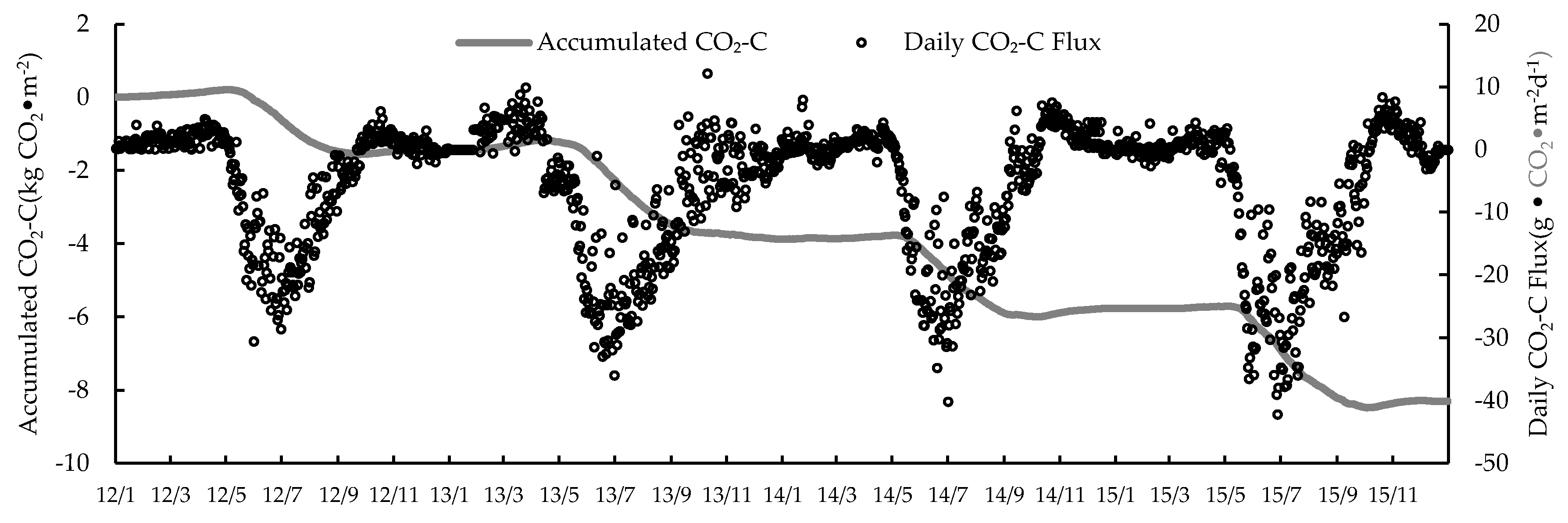
The CO2 concentration in the reed wetland ecosystem increased by 22.7 ppm from 2012 to 2015, which was below the global CO2 concentration. However, the annual average rate of increase was 5.67 ppm higher than the global rate (Table 2). The annual variation of the CO2 budget was large during the 4-year study period. The NEE absorption was 1472.97 g·CO2·m−2 in 2012, up to 2450.97 g·CO2·m−2 in 2015, and 1928.67 and 2296.84 g·CO2·m−2 in 2014 and 2013, respectively. The CO2 exchange accumulation curve suggests that the emissions in winter had little effect on the CO2 accumulation. The average annual CO2 absorption of reed wetland was 2037.15 g·m−2, which indicates a carbon sink (Figure 3). The seasonal variation trend of the CO2 exchange volume was similar in different years. The daily emission of CO2 gradually increased before the growth of reeds in the middle of April. From late April to May, the individual reeds were smaller and the CO2 absorption capacity was weaker. From June to July, the biomass of the reed was large, individual growth was at its highest, and the uptake of CO2 accounted for 67–78% of the year. The maximum daily absorption flux was 27.17 g·CO2·m−2·d−1 on 26 June 2012; 32.60 g·CO2·m−2·d−1 on 22 June 2013; 40.19 g·CO2·m−2·d−1 on 1 July 2014; and 42.20 g·CO2·m−2·d−1 on 27 June 2015. Soil respiration increased in August and September, with an increase in temperature, while the vegetative growth of the reed transformed into reproductive growth, and the CO2 net absorption of the reed community gradually decreased. From January to February, CO2 emissions were not significant, soil organic matter decomposition was slow, and soil respiration caused weak CO2 emissions from wetlands.
Based on the definition by Sagerfors (2007) [44] of the growing season (first day in the period when the 7-day average daily fluxes indicate stable uptake) as a period of net uptake, its length was 142 days in 2012 (5 May to 24 September), 161 days in 2013 (18 April to 26 September), 148 days in 2014 (5 May to 30 September) and 149 days in 2015 (7 May to 3 October).
3.2. Seasonal and Inter-Annual Variation of the Atmospheric Measurements
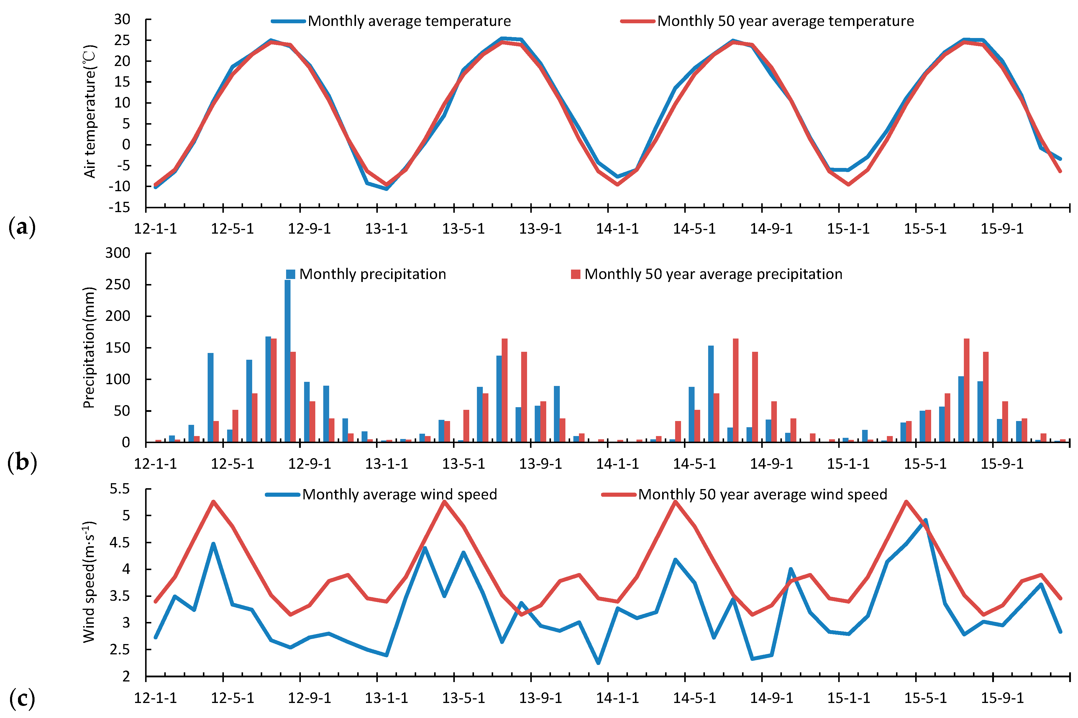
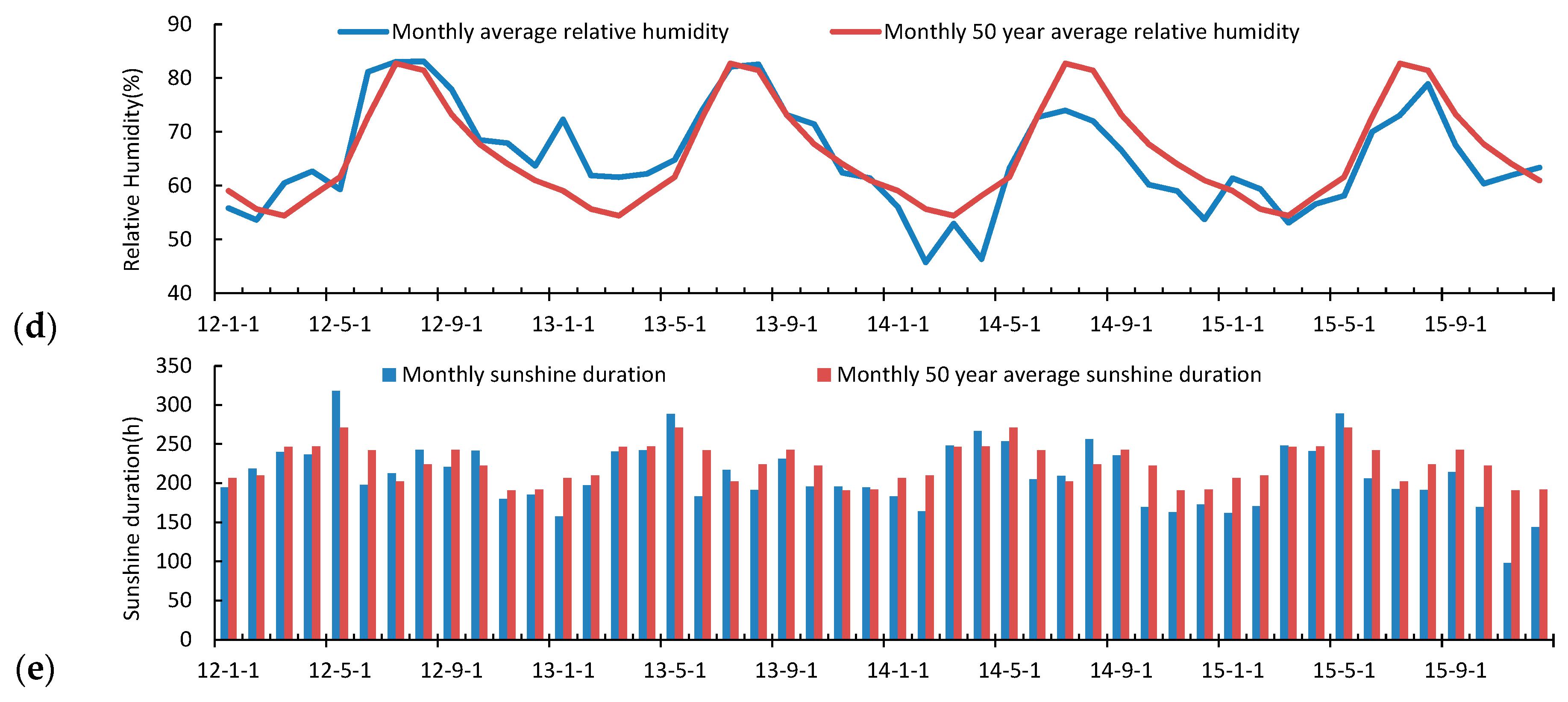
The average temperature (Ta) in 2012 (8.88 °C) was 0.04 °C lower than the Ta over the last 50 years (1961–2010; Table 3). In 2015, the annual Ta measured 10.26 °C, the highest in nearly 50 years. In 2012, the annual cumulative precipitation (PPT) anomalies measured 999 mm, and there were 98 PPT days. The PPT during 2013–2015 was 111.4 mm, 260.8 mm, and 164.1 mm, respectively, which were less than the long-term average of 611.2 mm. The relative humidity during 2012–2013 was higher than the long-term average of 65.97%. The average wind speed for the 4 years was less than the long-term average (3.93 m·s−1). The annual average sunshine duration (SD) from 2012 to 2015 was 2688.2 h, 2534.8 h, 2525.9 h, and 2326.8 h less than SD long-term average, respectively. The order of meteorological factors for the wetland during 2012–2015 was Ta rise, PPT, WS, RH, and SD decrease. The monthly variation of meteorological factors was clear, with the highest average monthly temperature in July and August, and the lowest in January (Figure 4). In the 4-year study period, temperatures in the winter and spring rose significantly, causing an increase in the annual average temperature. Rainfall was concentrated mainly from July to August. The precipitation and frequency during June, July, and August in 2012 were higher. The total annual precipitation in 2014 was the lowest, but the monthly precipitation in May and June was higher than the 50-year average. The precipitation from summer to winter during 2013–2015 was significantly lower than the long-term synchronization. The average wind speed had two peaks in spring and autumn, with the highest wind speed in April, the lowest in August, where the average wind speed of each month was less than the 50-year average. The average relative humidity was the highest in March and August, and lowest in December. In 2014, the relative humidity per month was less than the 50-year average. The longest SD months were May and September. In the autumn and winter, haze conditions reduced the number of sunshine hours, resulting in less ground-heat loss, and a smaller rise in the winter temperature.
3.3. Seasonal and Inter-Annual Variation of Phragmites Communis
From 2012 to 2015, the height of the reed canopy increased (Figure 5). The germination times of the reed occurred in mid-to-late April. The plant height and biomass increased linearly after germination, and the photosynthetic biomass of the reed increased a little until July. After August, the biomass again increased linearly. At this time the leaf area index decreased, and the weight of the stem increased. There was mainly vegetative growth, the dry matter in the leaves transferred to the stem, the biomass growth rate increased abruptly, and the plant height increased. The plant height and biomass reached a maximum in August or September. In September, the reed entered the flowering period, and the ground biomass decreased abruptly. After October, the reed entered the withering period, the average height of the stem was approximately 200 cm, and the average height of the reed stubble was approximately 15 cm in the following year.
3.4. Seasonal and Inter-Annual Variation of Soil Water and Salinity
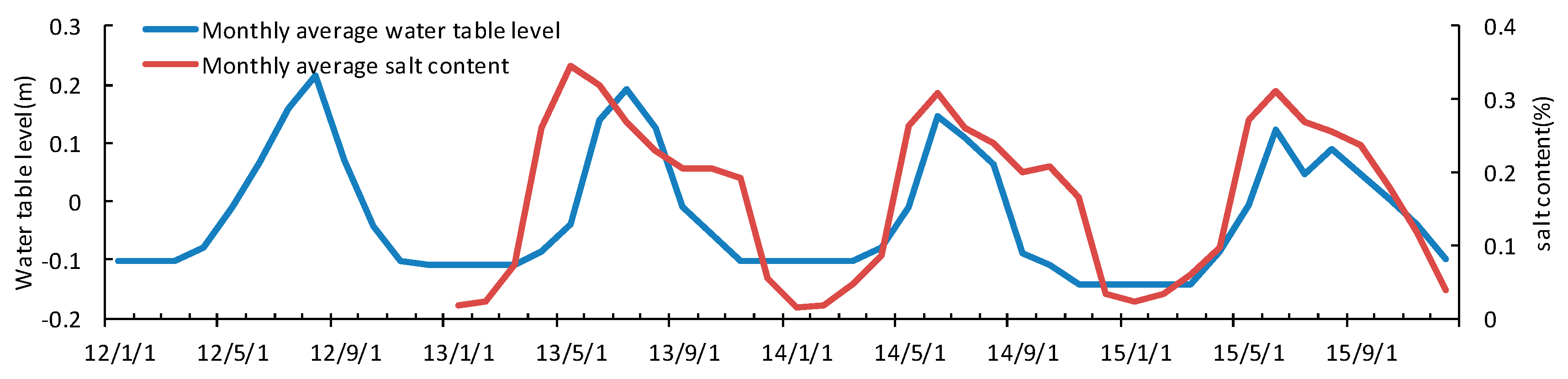
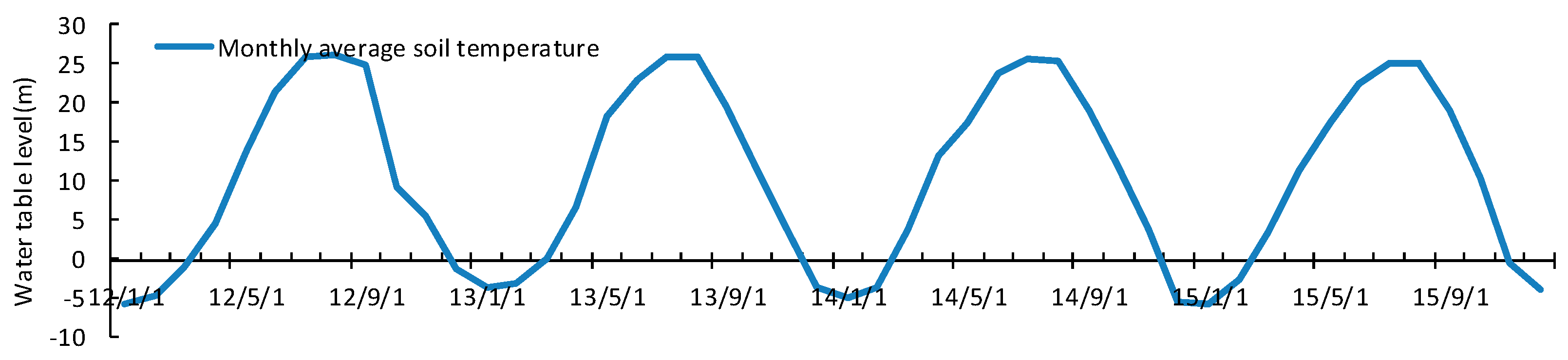
The WTL is the distance from the surface of the mud to the surface of the water, which is one of the key parameters that control the carbon budget of the wetland ecosystem [45]. The thickness of the WTL is related to the annual quota of artificial irrigation and precipitation recharge. The mean WTL during the growing season was 15 ± 6.2 cm, 11.3 ± 7.3 cm, 4.4 ± 5.0 cm, and 8.1 ± 6.8 cm below the vegetation surface in the years 2012, 2013, 2014, and 2015, respectively. During the growing season, the WTL trend was downward, with the lowest WTL in 2014 at 0.044 cm (Figure 6). The decrease in precipitation in summer and autumn were the cause of the WTL decrease in 2014 and 2015. The trend of salinity change had some correlation with the change in WTL thickness, which indicates that irrigation and drainage had a regulatory effect on salinity. The salinity was less than 0.1% before April. From May, the salinity increased rapidly, reaching 0.3%. The reed absorbed the dissolved salts as it grew, and the salinity then gradually decreased [46]. The process of rainwater top-down leaching also reduced the salinity. The variation curve of soil temperature was similar to that of air temperature. In the 4-year study period, Soil temperatures in the spring rose significantly (Figure 7).
3.5. Relationship between Environmental Factors and CO2
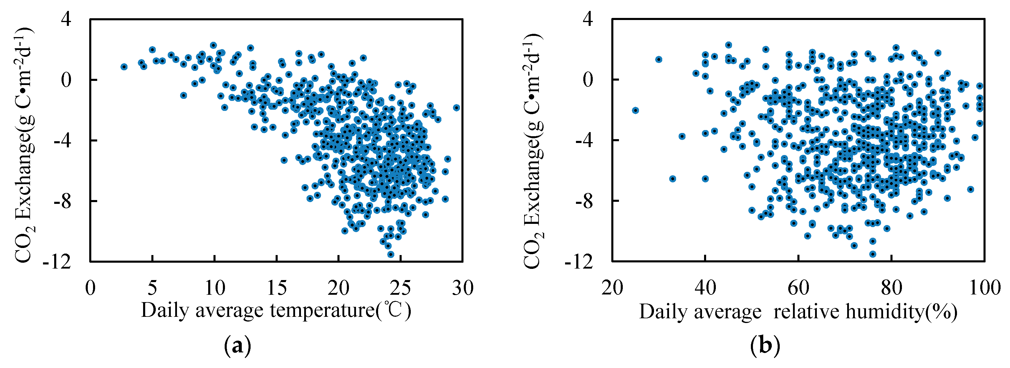
The relationship between the environmental factors and the monthly average CO2 (Figure 8) showed that the monthly CO2 exchange increased with increasing temperature when the temperature was below 10 °C. When the average temperature reached 10 °C, the absorption of CO2 began to increase linearly. The monthly precipitation ranged between 0 mm and 150 mm, and the CO2 exchange increased with increasing precipitation. Above 150 mm, the CO2 exchange decreased with increasing precipitation.
CO2 exchange was relative to the relative humidity, but the relative trend of wind speed and sunshine were not clear. The CO2 exchange was linearly related to the thickness of the water table layer. When the thickness was less than 0 cm, CO2 was weakly discharged. When the thickness ranged between 0 cm and 20 cm, CO2 was absorbed. Within a specific range, the increasing thickness of the water layer promoted the absorption of CO2. Within a salinity range of 0–0.2%, CO2 emissions increased with increasing salinity. Between 0.2% and 0.3%, CO2 absorption increased with increasing salinity.
On the basis of the monthly average, we further analyzed the relationship between the daily average and the environmental factors (Figure 9) in the growing season. Figure 9 and Figure 10 show a similar trend. The daily average correlation of air temperature, WTL, salinity, soil temperature and CO2 was more obvious. The maximum daily absorption of CO2 reached 12 g·C·m−2, when the temperature range was 20–25 °C, the water layer thickness was 0.1–0.2 m, the salinity was 0.3, and the soil temperature range was 20–25 °C.
The environmental factors attributed to CO2 exchange were studied using the PLS method. The VIP value of the WTL, soil salinity, temperature, weather, air temperature, precipitation, relative humidity, and biomass were greater than 0.8 (Figure 10), which had significant explanatory meaning for monthly CO2 exchange. The VIP of the WTL was maximum at 1.42, followed by surface soil temperature and air temperature. The VIP of the sunshine duration and wind speed were smaller, suggesting that the monthly CO2 balance did not have significant explanatory meaning. Environmental factors may have multiple collinearity and, therefore, we gathered collinearity statistcs for the environmental factors. When 0 < VIF < 10 and tolerance > 0.1, there is no multicollinearity; when 10 ≤ VIF < 100 and tolerance < 0.1, there is clear collinearity [47]. The results show that t2 and t3, t7 and t8 have clear collinearity (Table 4).
Using the PLS method, the environmental factors were divided into five groups to simulate the ability of the different combinations to explain the balance of CO2.
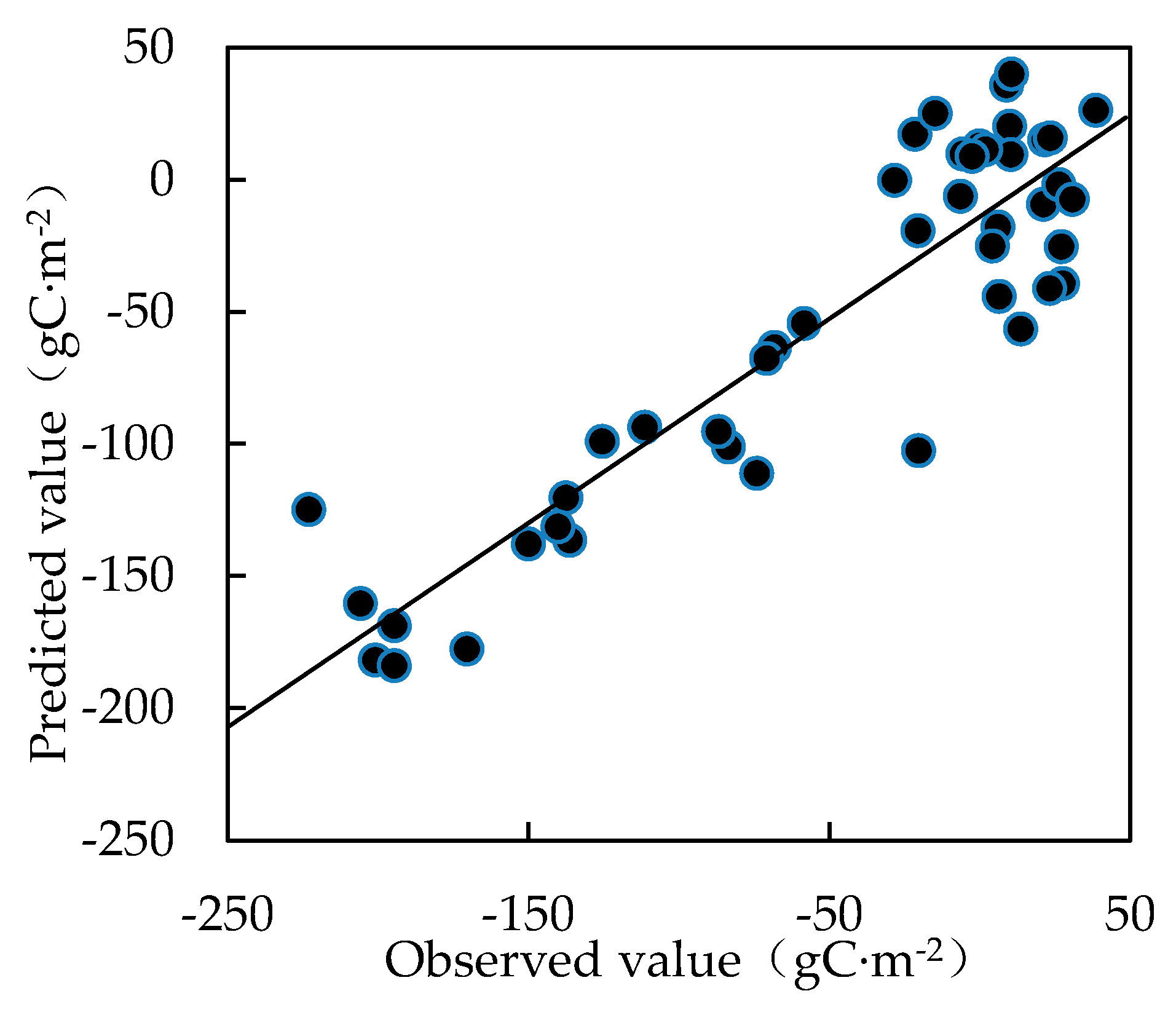
The first group, which included 10 environmental factors using the independent variable information rate R2X (cum) was the lowest, with a prediction accuracy of 62.9% (Table 4). The fifth group contained the VIP > 0.8 environmental factors, and the sixth group further eliminated the collinearity factor soil temperature. The ability and prediction accuracy of the sixth group was the best. The accuracy of the model increased from 62.9% to 72.5% (Table 5). This indicated that the model had 71.1% to 78.1% predictive power of CO2 exchange. The factors of the fifth group were used to predict the mathematical model of the CO2 monthly exchange, with a formula of Y = −0.588 − 0.647t1 − 0.356t3 + 0.028 t4 − 0.243t5 + 0.29t6 + 0.255t7. The predicted value of CO2 exchange is less than the observed value (Figure 11), with a correlation coefficient, R2 = 0.781.
4. Discussion
In this study, we used the eddy correlation method to analyze the CO2 exchange during 2012–2015 of the reed wetland in the Liaohe Delta, and observed the characteristics of several environmental factors simultaneously. The results showed that the atmospheric CO2 concentration increased annually. During the 4 years, the Liaohe Delta wetland was a large carbon sink. The average annual CO2 absorption was 2.04 kg·CO2·m−2, and the absorption peak was 23.51 µmol·m−2·s−1. The solid carbon capacity is higher than that of the Chongming Island wetland [48] and the Yellow River Delta [49]. The weak release period occurred from November to April and the net absorption period from May to October. The net absorption period was the longest in 2013, reaching 161 days. From June to July, the amount of CO2 absorption accounted for 62.11–78.54% of the year. The CO2 emissions were higher in April and September, reaching 7.35 g·CO2·m−2·d−1, and emissions were the lowest in December and January.
The annual average temperature during the 4–year period increased each year, and was clearly higher than that of the past 50 years, mainly owing to increased temperatures in winter. During 2013–2015, the accumulated annual precipitation was less than that for a normal year, especially during July–September; however, this did not affect the natural growth of the reeds. The annual sunshine duration decreased during 2012–2015. The decrease in the sunshine duration occurred mainly in winter, which had no effect on the absorption of CO2 by photosynthesis during the growing season of the reed.
There was correlation between environmental factors and CO2 exchange. The temperature range of 20–25 °C promotes photosynthesis of the reed. The WTL is one of the key control parameters of CO2 exchange, where the optimum depth is 0.1–0.2 m. Within a range of 0–0.2%, the increase in salinity can promote microbial activity, and increase organic carbon mineralization and CO2 emission. The salinity range of 0.2% to 0.8% is suitable for reed growth. At levels less than 0.2%, rush growth is too high, affecting the growth of the reeds.
The correlation of air temperature, WTL, salinity, soil temperature and CO2 was clearer than that of other factors. Water level and salinity are mainly affected by manual management measures. To increase the yield of the reeds, there should be initial irrigation, spring irrigation, and autumn irrigation according to the scientific irrigation of reed wetlands, where normal should be the “three irrigation, three rows” irrigation-management system. The first irrigation generally occurred from 10 March to 10 April. The main role of this was to advance thawing, increase the spring bud rate, and ensure the normal growth of the reeds. The spring irrigation was generally from 10 May to 10 June, where the main aim was to promote growth. Autumn irrigation generally occurred from 10 to 20 September to increase the reed fiber content and improve dry matter, while cultivating autumn buds, to lay the foundation for the second year of reed growth. The current water resources in the Liaohe Delta are mainly used for living and agriculture, and the remaining water can sustain a single spring irrigation, causing the single peak in the WTL curve. Over the 4-year period, the water supply for this irrigation management of “one irrigation and one row” was sufficient for the growth of reeds. During the last 3 years, precipitation in the Liaohe Delta decreased, and the decrease of the water layer had a positive effect on the uptake of CO2 in the reed wetland. Under irrigation management, the salinity of the growing season in the area was maintained within a range of 0.2–0.3%, which was favorable for the growth of reed and the promotion of CO2 absorption. The salinity tolerance range of reed (1.2–6.6 ng/L) [46] was better adapted to the salt marsh than that of the other types of wetland plants, such as Spartina alterniflora and Suaeda salsa.
The PLS regression model overcomes the shortcomings of traditional regression analysis, and dynamically quantifies the relationship between CO2 absorption and environmental factors in reed wetlands. Variable importance in projection reflects the importance of environmental factors for the CO2 exchange. The thickness of the water layer had the strongest effect on the CO2 exchange, followed by soil temperature, temperature, and salinity, whereas wind speed and sunshine had little effect. Therefore, irrigation is the best way to adjust the carbon balance of the reed. Independent variables such as soil water and salinity, and weather, can simulate and explain the CO2 exchange. This indicates that WTL and temperature are the main environmental factors that determine the distribution of reeds, ecotypes, and growth conditions [21].
5. Conclusions
The Liaohe Delta wetland is a large carbon sink. It plays an important role in wetland carbon sequestration in China. The variability of the CO2 exchange over the past four years was affected by vegetation and meteorological and hydrological factors. The changes in the environmental factors include increasing temperature, decreasing precipitation and sunshine hours, and increasing CO2 concentration.
Owing to the aforementioned environmental changes and irrigation management, the ability of the reeds to absorb CO2 and convert it to organic carbon was enhanced, reflecting the ability of the reeds to adapt to the environment. The WTL was the main contributor to the carbon dioxide expenditure among environmental factors. Satisfactory results were achieved using the PLS method to simulate carbon dioxide.
In recent years, under increasing temperatures and decreasing precipitation, artificial irrigation has controlled the key WTL, and can increase the CO2 absorption in the growing season. However, the increased temperatures in winter lead to increased emissions. The effect of coupling between the water level and salinity, and meteorological factors on the carbon balance of the wetland, will be the focus of future research.
Acknowledgments
This study is supported by the National Natural Science Foundation of China (41405109, 41375146), the Research project of Liaoning Meteorological Bureau (BA201607) and the Foundation of the Institute of Atmospheric Environment (2016SYIAEZD2, 2017SYIAEMS2). We thank Reetta Saikku, from Liwen Bianji, Edanz Editing China (www.liwenbianji.cn/ac), for editing the English text of a draft of this manuscript. Also, we would like to thank the Panjin Wetland Research Base for all data of the case study. The authors are grateful to all participants in the field for their contributions to the progress of this study.
Author Contributions
Qingyu Jia contributed to the conception and design, data analysis and interpretation, draft and revision of the manuscript. Wenying Yu collected the data. Li Zhou and Chenghua Liang contributed to the draft of the manuscript.
Conflicts of Interest
The authors declare no conflict of interest.
References
- Davidson, N.C. How much wetland has the world lost? Long-term and recent trends in global wetland area. Mar. Freshw. Res. 2014, 65, 934–941. [Google Scholar] [CrossRef]
- Mitsch, W.J.; Bernal, B.; Nahlik, A.M.; Mander, Ü.; Zhang, L.; Anderson, C.J. Wetlands, carbon, and climate change. Landsc. Ecol. 2012, 28, 1–15. [Google Scholar] [CrossRef]
- Solomon, S.; Qin, D.H.; Manning, M. Climate Change 2007: The Physical Science Basis; Contribution of Working Group I to the Fourth Assessment Report of the Intergovernmental Panel on Climate Change; Cambridge University Press: Cambridge, UK; New York, NY, USA, 2007. [Google Scholar]
- Yu, Z. Holocene carbon flux histories of the world’s peatlands: Global carbon-cycle implications. Holocene 2011, 21, 761–774. [Google Scholar] [CrossRef]
- Charman, D.J.; Beilman, D.W.; Blaauw, M.; Booth, R.K.; Brewer, S.; Chambers, F.M. Climate-related changes in peatland carbon accumulation during the last millennium. Biogeosci. Discuss. 2012, 9, 929–944. [Google Scholar] [CrossRef] [Green Version]
- Bu, Z.; Hans, J.; Li, H.; Zhao, G.; Zheng, X.; Ma, J.; Zeng, J. The response of peatlands to climate warming: A review. Acta Ecol. Sin. 2011, 31, 157–162. [Google Scholar] [CrossRef]
- Nilsson, M.; Sagerfors, J.; Buffam, I.; Laudon, H.; Eriksson, T.; Grelle, A.; Klemedtsson, L.; Weslien, P.; Lindroth, A. Contemporary carbon accumulation in a boreal oligotrophic minerogenic mire a significant sink after accounting for all C-fluxes. Glob. Chang. Biol. 2008, 14, 2317–2332. [Google Scholar] [CrossRef]
- Koehler, A.-K.; Sottocornola, M.; Kiely, G. How strong is the current carbon sequestration of an Atlantic blanket bog? Glob. Chang. Biol. 2015, 17, 309–319. [Google Scholar] [CrossRef]
- Kennedy, H.; Alongi, D.M.; Karim, A.; Chen, G.; Chmura, G.L.; Crooks, S. Chapter 4 coastal wetlands. In 2013 Supplement to the 2006 IPCC Guidelines for National Greenhouse Gas Inventories: Wetlands; IPCC: Geneva, Switzerland, 2014. [Google Scholar]
- Baldocchi, D.D. Assessing the eddy covariance technique for evaluating carbon dioxide exchange rates of ecosystems: Past, present and future. Glob. Chang. Biol. 2003, 9, 479–492. [Google Scholar] [CrossRef]
- Lund, M.; Lafleur, P.M.; Roulet, N.T.; Lindroth, A.; Christensen, T.R.; Aurela, M. Variability in exchange of CO2, across 12 northern peatland and tundra sites. Glob. Chang. Biol. 2010, 16, 2436–2448. [Google Scholar] [CrossRef]
- Kerkhoff, A.; Enquist, B.; Elser, J.; Fagan, W. Plant allometry, stoichiometry and the temperature-dependence of primary productivity. Glob. Ecol. Biogeogr. 2005, 14, 585–598. [Google Scholar] [CrossRef]
- Staehr, P.A.; Sand-Jensen, K. Seasonal changes in temperature and nutrient control of photosynthesis, respiration and growth of natural phytoplankton communities. Fresh Water Biol. 2006, 51, 249–262. [Google Scholar] [CrossRef]
- Flanagan, L.B. Stimulation of both photosynthesis and respiration in response to warmer and drier conditions in a boreal peatland ecosystem. Glob. Chang. Biol. 2011, 17, 2271–2287. [Google Scholar] [CrossRef]
- Gedan, K.B.; Bertness, M.D. How will warming affect the salt marsh foundation species Spartina patens and its ecological role? Oecologia 2010, 164, 479–487. [Google Scholar] [CrossRef] [PubMed]
- Kirwan, M.L.; Blum, L.K. Enhanced decomposition offsets enhanced productivity and soil carbon accumulation in coastal wetlands responding to climate change. Biogeosciences 2011, 8, 987–993. [Google Scholar] [CrossRef]
- Charles, H.; Dukes, J.S. Effects of warming and altered precipitation on plant and nutrient dynamics of a New England salt marsh. Ecol. Appl. Publ. Ecol. Soc. Am. 2009, 19, 1758. [Google Scholar] [CrossRef]
- Anna, M.A.; Jianjian, L.U. The Progress of research on carbon flux in wetland ecosystems. Wetl. Sci. 2008, 6, 116–123. [Google Scholar]
- Zhu, X.; Wang, S.; Zhang, C. Responses of different ecotypes of reed growing in the Hexi corridor to natural drought and salinity. Plant Physiol. J. 2003, 39, 371–376. [Google Scholar]
- Saenger, C.; Cronin, T.; Thunell, R.; Vann, C. Modelling river discharge and precipitation from estuarine salinity in the northern Chesapeake Bay: Application to Holocene palaeoclimate. Holocene 2006, 16, 467–477. [Google Scholar] [CrossRef]
- Vretare, V.; Weisner, S.E.B.; Strand, J.A.; Granéli, W. Phenotypic plasticity in Phragmites australis as a functional response to water depth. Aquat. Bot. 2001, 69, 127–145. [Google Scholar] [CrossRef]
- Zhao, K.; Li, J. Effects of salinity on the contents of osmotica of monocotyledenous halophytes and their contribution to osmotic adjustment. Acta Bot. Sin. 2009, 41, 1287–1292. [Google Scholar]
- Zhang, S.; Guo, C.; Su, F. Effect of salinity on the growth of reed. J. Shenyang Agric. Univ. 2008, 39, 65–68. [Google Scholar]
- Weston, N.B.; Vile, M.A.; Neubauer, S.C.; Velinsky, D.J. Accelerated microbial organic matter mineralization following salt-water intrusion into tidal freshwater marsh soils. Biogeochemistry 2011, 102, 135–151. [Google Scholar] [CrossRef]
- Bubier, J.; Crill, P.; Mosedale, A.; Frolking, S.; Linder, E. Peatland responses to varying interannual misture conditions as measured by automatic CO2 chambers. Glob. Biogeochem. Cycles 2003, 17, 1066–1081. [Google Scholar] [CrossRef]
- Chen, G. Study on Marsh in Sanjiang Plain; Science Press: Beijing, China, 1996; pp. 165–168. [Google Scholar]
- Minchinton, T.E. Disturbance by wrack facilitates spread of Phragmites australis in a coastal marsh. J. Exp. Mar. Biol. Ecol. 2002, 281, 89–107. [Google Scholar] [CrossRef]
- Robroek, B.J.M.; Schouten, M.G.C.; Limpens, J.; Berendse, F.; Poorter, H. Interactive effects of water table and precipitation on net CO2 assimilation of three co-occurring sphagnum mosses differing in distribution above the water table. Glob. Chang. Biol. 2009, 15, 680–691. [Google Scholar] [CrossRef]
- Daulat, W.E.; Clymo, R.S. Effects of temperature and watertable on the efflux of methane from peatland surface cores. Atmos. Environ. 1998, 32, 3207–3218. [Google Scholar] [CrossRef]
- Frolking, S.; Roulet, N.T. Holocene radiative forcing impact of northern peatland carbon accumulation and methane emissions. Glob. Chang. Biol. 2010, 13, 1079–1088. [Google Scholar] [CrossRef]
- Heinsch, F.A.; Heilman, J.L.; Mcinnes, K.J.; Cobos, D.R.; Zuberer, D.A. Carbon dioxide exchange in a high marsh on the Texas Gulf Coast: Effects of freshwater availability. Agric. For. Meteorol. 2004, 125, 159–172. [Google Scholar] [CrossRef]
- Fenner, N.; Freeman, C. Drought-induced carbon loss in peatlands. Nat. Geosci. 2011, 4, 895–900. [Google Scholar] [CrossRef]
- Han, G.; Yang, L.; Yu, J.; Wang, G.; Mao, P.; Gao, Y. Environmental Controls on Net Ecosystem CO2 Exchange Over a Reed (Phragmites australis) Wetland in the Yellow River Delta, China. Estuaries Coasts 2013, 36, 401–413. [Google Scholar] [CrossRef]
- Thomas, K.L.; Benstead, J.; Davies, K.L.; Lloyd, D. Role of wetland plants in the diurnal control of CH4 and CO2 fluxes in peat. Soil Biol. Biochem. 1996, 28, 17–23. [Google Scholar] [CrossRef]
- Mei, X.; Zhang, X. Carbon storage and fixation by a typical wetland vegetation in Changjiang River Estuary—A case study of Phragmites australis in east beach of Chongming Island. Chin. J. Eco-Agric. 2008, 16, 269–272. [Google Scholar] [CrossRef]
- Li, B.; Liu, C.-Q.; Wang, J.-X.; Zhang, Y.-J. Carbon Storage and Fixation Function by Phragmites australis, a Typical Vegetation in Baiyangdian Lake. J. Agro-Environ. Sci. 2009, 28, 2603–2607. [Google Scholar]
- Qi, Y. Study on the allocation scheme of multi-source ecological water supply of Panjin reed wetland. Water Resour. Hydropower Northeast China 2015, 33, 19–21. [Google Scholar]
- Sagerfors, J.; Lindroth, A.; Grelle, A.; Klemedtsson, L.; Weslien, P.; Nilsson, M. Annual CO2 exchange between a nutrient-poor, minerotrophic, boreal mire and the atmosphere. J. Geophys. Res. 2008, 113, G01001. [Google Scholar] [CrossRef]
- Lv, X. Wetland Ecosystem Observation Method; China Environmental Science Press: Beijing, China, 2005; pp. 94–99. [Google Scholar]
- Krishnan, A.; Williams, L.J.; Mcintosh, A.R.; Abdi, H. Partial least squares (PLS) methods for neuroimaging: A tutorial and review. Neuroimage 2011, 56, 455–475. [Google Scholar] [CrossRef] [PubMed]
- Wold, S.; Sjöström, M.; Eriksson, L. PLS-regression: A basic tool of chemometrics. Chemom. Intell. Lab. Syst. 2001, 58, 109–130. [Google Scholar] [CrossRef]
- Giuseppe, P.; Paolo, P.; Hans-Dieter, Z. Performance of PLS regression coefficients in selecting variables for each response of a multivariate PLS for omics-type data. Adv. Appl. Bioinform. Chem. 2009, 2, 57–70. [Google Scholar]
- Johnson, R.A.; Wichern, D.W. Applied Multivariate Statistical Analysis; Prentice Hall: New Jersey, NJ, USA, 2002. [Google Scholar]
- Sagerfors, J. Land-Atmosphere Exchange of CO2, Water and Energy at a Boreal Minerotrophic Mire. Ph.D. Thesis, Swedish University of Agricultural Sciences, Umea, Sweden, January 2007. [Google Scholar]
- Peichl, M.; Sonnentag, O.; Nilsson, M.B. Bringing color into the picture: Using digital repeat photography to investigate phenology controls of the carbon dioxide exchange in a boreal mire. Ecosystems 2014, 18, 115–131. [Google Scholar] [CrossRef]
- Sun, B.; Xie, J.C.; Wang, N.; Li, S.-Q.; Li, C.-J. Effect of reeds on salt enrichment and improvement of saline-alkali land. J. Soil Water Conserv. 2012, 26, 92–101. [Google Scholar]
- Hair, J.; Black, W.; Babin, B.; Anderson, R. Multivariate Data Analysis: Pearson New International Edition PDF eBook; Pearson: Zug, Switzerland, 2013; Volume 3, pp. 128–134. [Google Scholar]
- Li, Y.; Cui, L.; Pan, X.; Ning, Y.; Li, W.; Kang, X. Spatial distribution of plant diversity and functional groups in the Liaohe estuary. Biodivers. Sci. 2015, 23, 471–478. [Google Scholar] [CrossRef]
- Kang, X.M.; Cui, L.J.; Yue, X.L.; Li, W.; Zhang, M.Y.; Zhao, X.S.; Hao, Y.B.; Lei, Y.R.; Gao, Q. Valuation of Air Regulation by the Reed (Phragmites australis) Wetland in the Yellow River Delta. Wetl. Sci. Manag. 2015, 11, 23–25. [Google Scholar]
Figure 1.
Phenological phase of Phragmites communis.
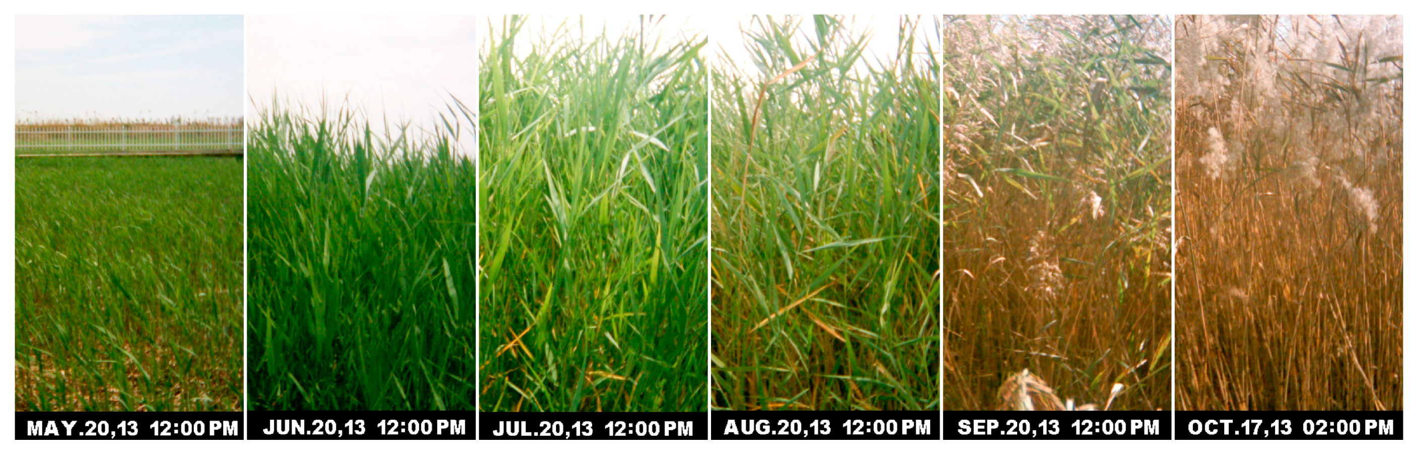
Figure 2.
EC observation system.
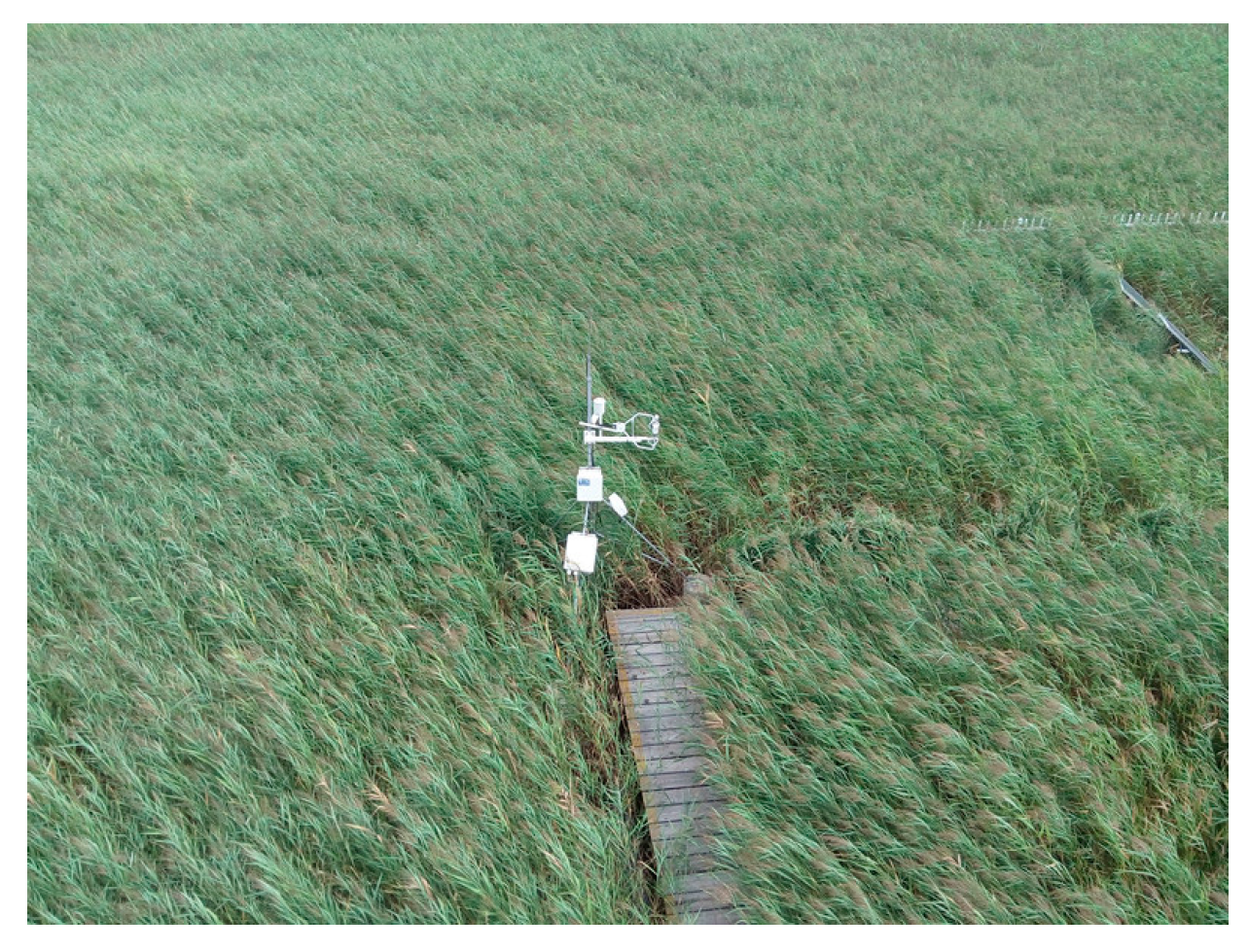
Figure 3.
Daily carbon fluxes over the 4-year study period, measured by the eddy covariance technique. Red dots indicate daily sums; and the blue line the accumulated curve.
Figure 3.
Daily carbon fluxes over the 4-year study period, measured by the eddy covariance technique. Red dots indicate daily sums; and the blue line the accumulated curve.

Figure 4.
Comparison of the meteorological elements with the 50-year average (1960–2010). (a) Temperature; (b) Precipitation; (c) Wind speed; (d) Relative humidity; (e) Sunshine duration.
Figure 4.
Comparison of the meteorological elements with the 50-year average (1960–2010). (a) Temperature; (b) Precipitation; (c) Wind speed; (d) Relative humidity; (e) Sunshine duration.


Figure 5.
Plant height and biomass change.

Figure 6.
Water table level (WTL) and salinity change.

Figure 7.
Topsoil temperature change.

Figure 8.
Environmental factors and CO2 monthly exchange. (a) Temperature; (b) Precipitation; (c) Relative humidity; (d) Wind speed; (e) Sunshine duration; (f) Water table level; (g) Salt content; (h) Soil temperature.
Figure 8.
Environmental factors and CO2 monthly exchange. (a) Temperature; (b) Precipitation; (c) Relative humidity; (d) Wind speed; (e) Sunshine duration; (f) Water table level; (g) Salt content; (h) Soil temperature.
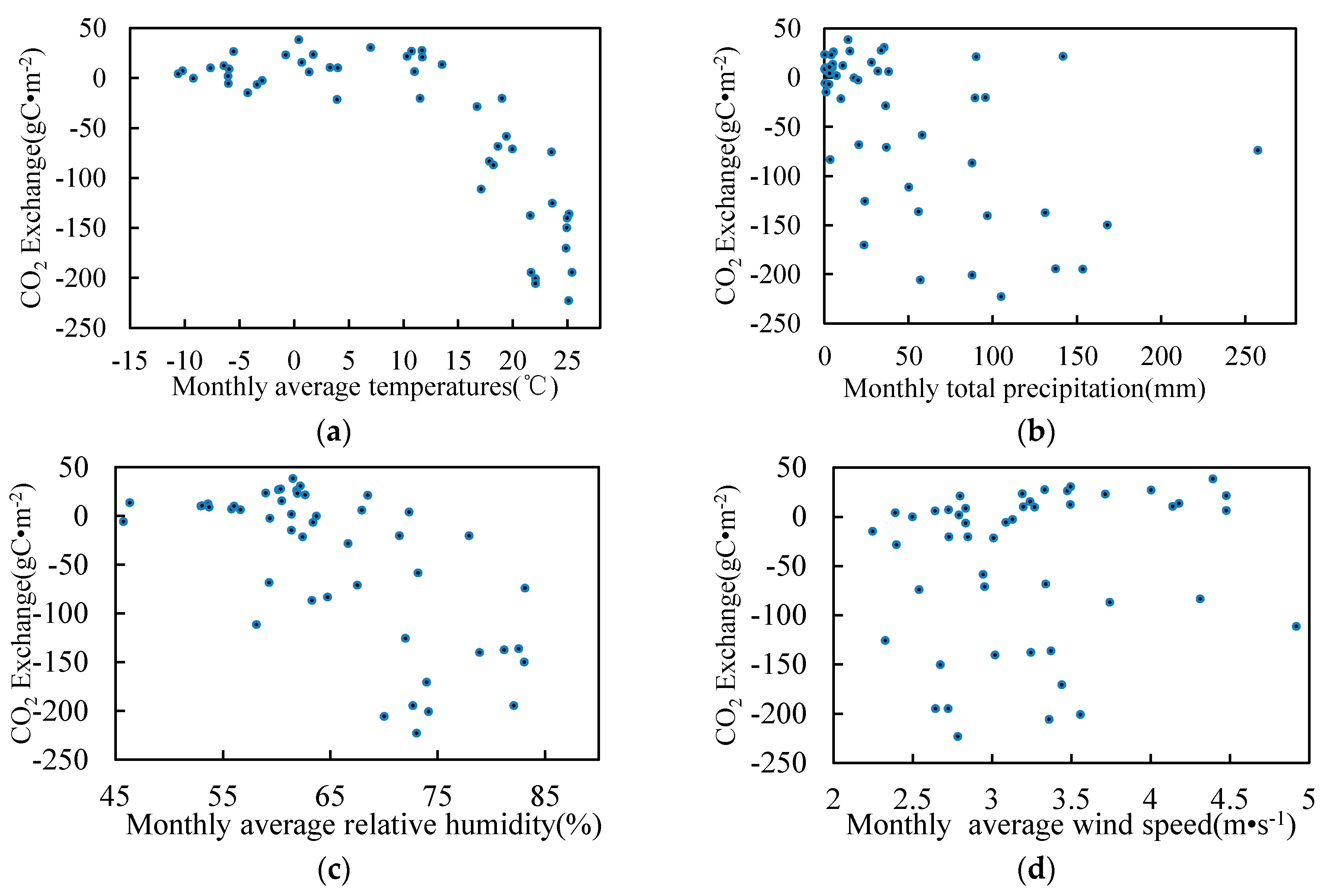
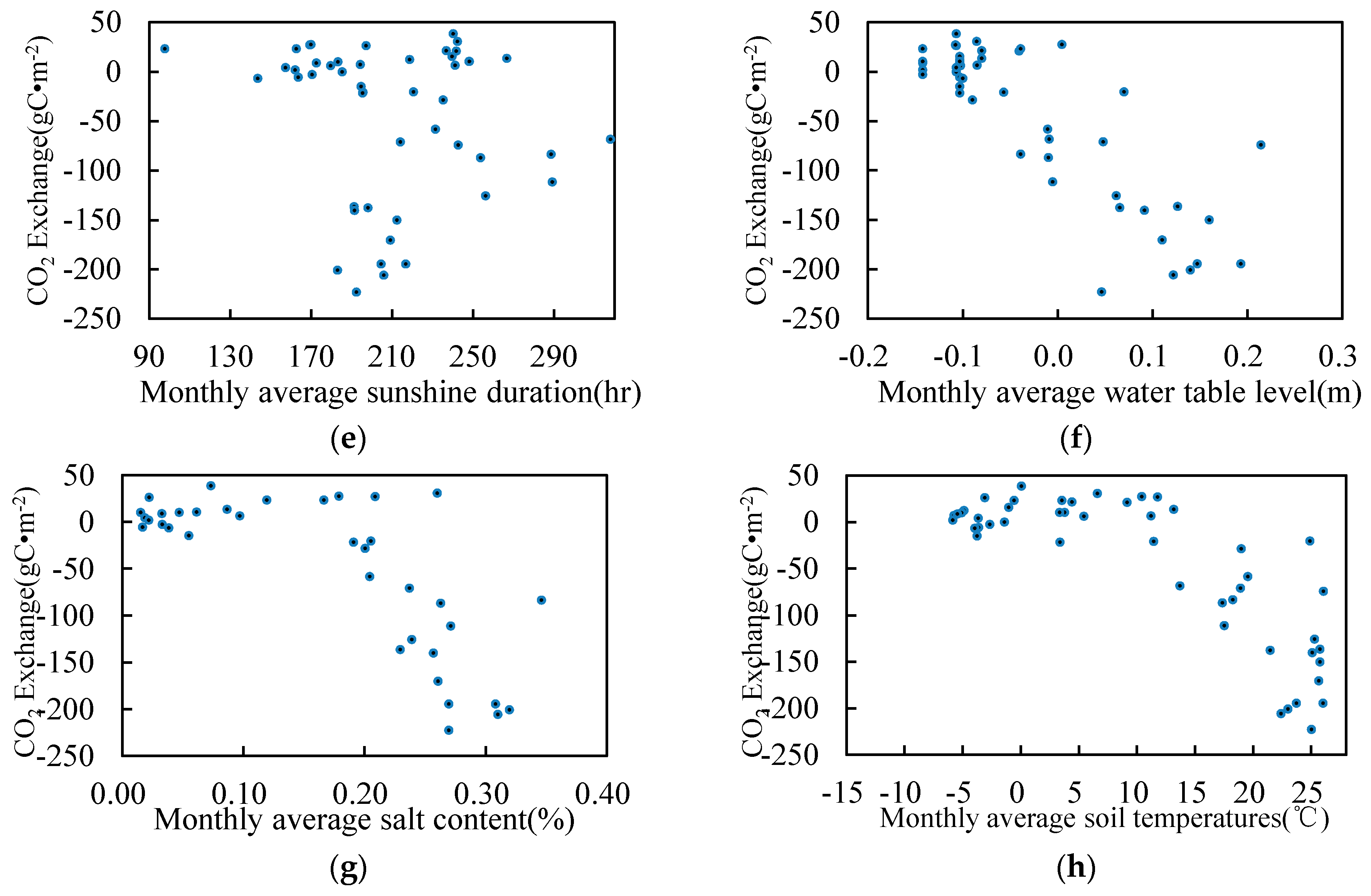
Figure 9.
Environmental factors and CO2 daily exchange in the growing season. (a) Temperature; (b) Relative humidity; (c) Wind speed; (d) Sunshine duration; (e) Water table level; (f) salt content; (g) Soil temperature.
Figure 9.
Environmental factors and CO2 daily exchange in the growing season. (a) Temperature; (b) Relative humidity; (c) Wind speed; (d) Sunshine duration; (e) Water table level; (f) salt content; (g) Soil temperature.

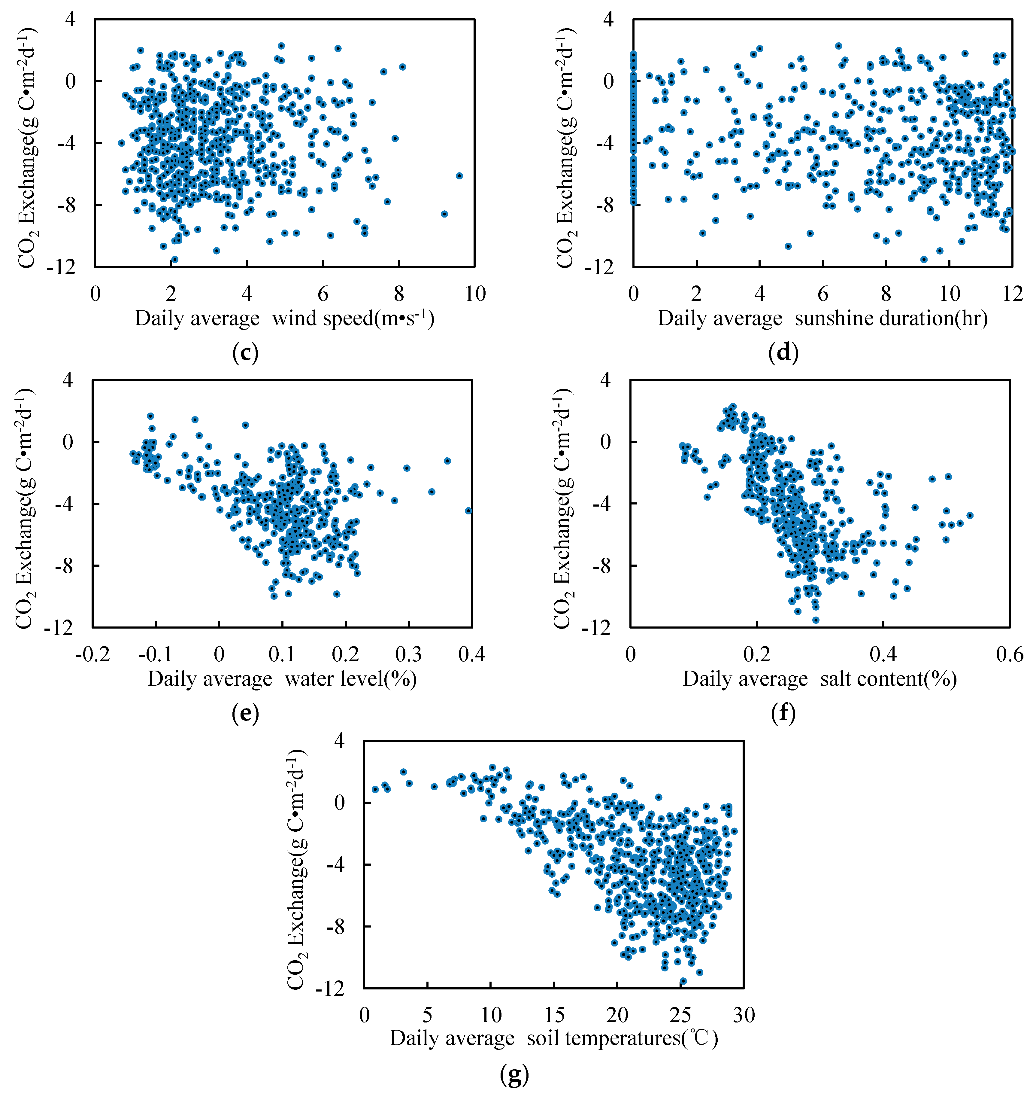
Figure 10.
Variable importance in projection (VIP) of the environmental factors for CO2 exchange. t1 is the WTL, t2 is soil temperature; t3 is air temperature; t4 is the salt content; t5 is relative humidity; t6 is precipitation; t7 is biomass; t8 is sunshine duration; t9 is height; and t10 is wind speed.
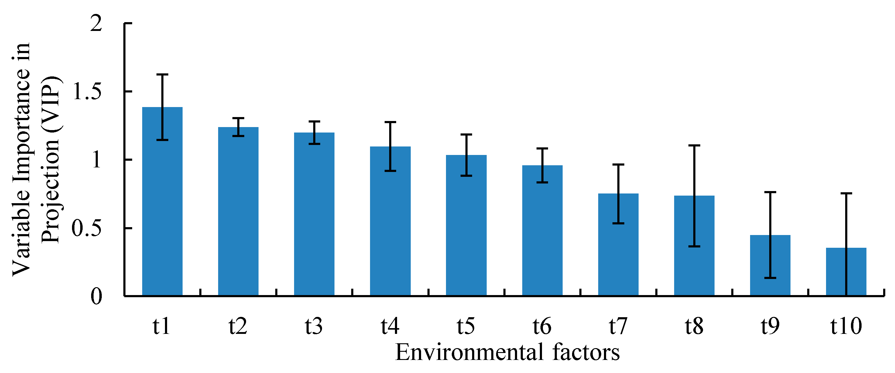
Figure 11.
Scatter plots of the observed and simulated values of CO2 monthly exchange.


Table 1.
Soil physical chemical properties.
| Depth (cm) | pH | Organic Matter (g·kg−1) | Total N (g·kg−1) | Nitrate N (mg·kg−1) | Ammonium N (mg·kg−1) | Alkali-Hydrolysis N (mg·kg−1) | Total P (mg·kg−1) | Available P (mg·kg−1) | Total K (g·kg−1) | Available K (g·kg−1) | C/N |
|---|---|---|---|---|---|---|---|---|---|---|---|
| 0–20 | 8.80 ± 0.2 | 19.4 ± 10 | 1.55 ± 0.1 | 4.21 ± 1.4 | 14.75 ± 6.0 | 67.2 ± 26 | 35 ± 6 | 14.50 ± 0.7 | 2.86 ± 0.3 | 0.75 ± 0.05 | 6.8 ± 1.6 |
| 20–40 | 9.27 ± 0.1 | 9.8 ± 3 | 1.65 ± 0.1 | 6.24 ± 0.9 | 4.33 ± 0.5 | 30.8 ± 14 | 22.62 ± 1.4 | 0.83 ± 0.32 |
Table 2.
CO2 concentration characteristics.
| Year | Reed Wetland (ppm) | Standard Deviation SD |
|---|---|---|
| 2012 | 375.14 | 24.67 |
| 2013 | 366.78 | 21.76 |
| 2014 | 383.65 | 11.90 |
| 2015 | 397.84 | 14.77 |
Table 3.
Meteorological factors and 50-year average comparison for 2012–2015.
| Year | Ta (°C) | PPT (mm) | RH (%) | Sunshine Duration (h) | WS (m·s−1) |
|---|---|---|---|---|---|
| 2012 | 8.88 | 999 | 68.13 | 2688.2 | 3.03 |
| 2013 | 9.48 | 499.8 | 69.22 | 2534.8 | 3.22 |
| 2014 | 9.71 | 350.4 | 60.32 | 2525.9 | 3.20 |
| 2015 | 10.26 | 447.1 | 63.67 | 2326.8 | 3.45 |
| 1961–2010 | 8.92 ± 0.73(±SD) | 611.2 ± 158.3(±SD) | 65.97 ± 2.47(±SD) | 2697.6 ± 192.3(±SD) | 3.93 ± 0.65(±SD) |
Table 4.
Collinearity statistics.
| Factors | Tolerance | VIF |
|---|---|---|
| t1 | 0.150 | 6.673 |
| t2 | 0.017 | 57.506 |
| t3 | 0.017 | 59.054 |
| t4 | 0.405 | 2.471 |
| t5 | 0.104 | 9.629 |
| t6 | 0.451 | 2.215 |
| t7 | 0.087 | 11.540 |
| t8 | 0.361 | 2.770 |
| t9 | 0.070 | 14.303 |
| t10 | 0.274 | 3.653 |
Table 5.
Environmental factors that explain the CO2 amount.
| Factor | R2X (cum) | R2Y (cum) | Q2 (cum) |
|---|---|---|---|
| The first group (Total factors) | 0.567 | 0.647 | 0.629 |
| The second group (Tair, P, RH) | 0.9 | 0.621 | 0.574 |
| The third group (WTL, SAL, TSoil) | 0.9 | 0.673 | 0.661 |
| The fourth group (H, Biomass) | 0.907 | 0.162 | 0.091 |
| The fifth group (Tair, P, RH, WTL, SAL, Tsoil, Biomass) | 0.885 | 0.781 | 0.711 |
| The sixth group (Tair, P, RH, WTL, SAL, Biomass) | 0.0898 | 0.781 | 0.725 |
© 2017 by the authors. Licensee MDPI, Basel, Switzerland. This article is an open access article distributed under the terms and conditions of the Creative Commons Attribution (CC BY) license (http://creativecommons.org/licenses/by/4.0/).
Share and Cite
MDPI and ACS Style
Jia, Q.; Yu, W.; Zhou, L.; Liang, C. Atmospheric and Surface-Condition Effects on CO2 Exchange in the Liaohe Delta Wetland, China. Water 2017, 9, 806. https://doi.org/10.3390/w9100806
AMA Style
Jia Q, Yu W, Zhou L, Liang C. Atmospheric and Surface-Condition Effects on CO2 Exchange in the Liaohe Delta Wetland, China. Water. 2017; 9(10):806. https://doi.org/10.3390/w9100806
Chicago/Turabian StyleJia, Qingyu, Wenying Yu, Li Zhou, and Chenghua Liang. 2017. "Atmospheric and Surface-Condition Effects on CO2 Exchange in the Liaohe Delta Wetland, China" Water 9, no. 10: 806. https://doi.org/10.3390/w9100806
Note that from the first issue of 2016, this journal uses article numbers instead of page numbers. See further details here.