Article

Discharge Fee Policy Analysis: A Computable General Equilibrium (CGE) Model of Water Resources and Water Environments

1
College of Water Conservancy and Hydropower Engineering, Hohai University, Nanjing 210098, China
2
Bureau of Comprehensive Development, Ministry of Water Resources, Beijing 100000, China
3
Construction and Administration Bureau of South-to-North Water Diversion Middle Route Project, Beijing 100038, China
*
Author to whom correspondence should be addressed.
Water 2016, 8(9), 413; https://doi.org/10.3390/w8090413
Submission received: 4 June 2016 / Revised: 9 August 2016 / Accepted: 7 September 2016 / Published: 21 September 2016
(This article belongs to the Special Issue Water Economics and Policy)

Abstract

:
To alleviate increasingly serious water pollution and shortages in developing countries, various kinds of policies have been implemented by local governments. It is vital to quantify and evaluate the performance and potential economic impacts of these policies. This study develops a Computable General Equilibrium (CGE) model to simulate the regional economic and environmental effects of discharge fees. Firstly, water resources and water environment factors are separated from the input and output sources of the National Economic Production Department. Secondly, an extended Social Accounting Matrix (SAM) of Jiangsu province is developed to simulate various scenarios. By changing values of the discharge fees (increased by 50%, 100% and 150%), three scenarios are simulated to examine their influence on the overall economy and each industry. The simulation results show that an increased fee will have a negative impact on Gross Domestic Product (GDP). However, waste water may be effectively controlled. Also, this study demonstrates that along with the economic costs, the increase of the discharge fee will lead to the upgrading of industrial structures from a situation of heavy pollution to one of light pollution which is beneficial to the sustainable development of the economy and the protection of the environment.

1. Introduction

Water pollution and shortages represent two major water crises around the world. In developing counties, these issues are becoming increasingly serious due to the explosive growth of the population and significant advancements in social-economic development, which pose many negative impacts on people’s health and the sustainable development of regions.
Traditional input-output (I-O) approaches and Computable General Equilibrium (CGE) models are only based on economic systems, which calculate production and consumption of an economy, without considering water resources, water environmental damage or appropriate protection activities. A CGE model which can be considered as a set of linear or nonlinear equations is utilized to demonstrate comprehensive relationships between supply and demand of various commodities and production factors in an economic system [1]. The environmental CGE models examine coordinated developments of the relationship among society, economy and environment under the shock of varied policies. The environmental CGE model has been widely used because it can fully reflect chain reactions and feedback effects in the process of policy implementation [2]. Bergman developed a static CGE model with seven sectors to evaluate the effects of air pollution control policy in Sweden. His results showed the general equilibrium effects between emission behaviors and mitigation actions [3]. Piggott et al. developed a static multinational CGE model about international trade and carbon emission to analyze the international effects of carbon tax [4]. Llop and Ponce-Alifonso employed a CGE model to analyze two of the main challenges faced by agriculture in Europe: technological changes and the application of the principle of cost recovery to water services [5]. CGE model structures have been tailored to include environmental feedbacks on the economic system. Robinson incorporated the net emissions into Stone-Geary function [6]. Besides modifications of production function and consumption function, production functions of pollution control behaviors and technologies have been listed [7]. In fact, these early studies treated the water sector as a passive rather than an active agent responsible for the provision of usable water. There have been many studies using CGE models to explore water issues. In these studies, water resources were considered in the CGE models as a production factor which provided resources for various industries, or as a type of constraint which restrained industrial development. Seung et al. found that the SAM model overestimated the agricultural sector’s outputs and factor income by comparing it with the social accounting matrix (SAM) model in researching agricultural transfer of water [8]. Furthermore, Seung et al. proposed a dynamic CGE model consisting of three agricultural sectors and five non-agricultural sectors to investigate the economic impacts of water being transfered from agriculture to wetlands [9,10]. A recent extension was to integrate a CGE model by linking it with a water management model, which allowed for a finer depiction of water distributions within irrigated agriculture. Water resource utilization was included in the model in terms of agricultural sectors by way of water shocks such as droughts, and then the impacts on gross domestic product (GDP) and household income were modeled [11].
The different water prices for consumers have led to the development of numerous models that assessed the impacts of different pricing policies. Decaluwé et al. used a CGE model to examine the impacts of different water pricing policies on agriculture and other industries. Due to the higher subsidies given to agriculture in the base period, there were stronger effects on the industry after simulating the water pricing policies and the agriculture sector had no flexible capital flow to deal with the changing policies. As a result, the agriculture sector was more greatly affected by the water pricing policies than other industries [12,13]. Gómez et al. presented a CGE model to analyze the welfare gains associated with an improvement in the allocation of water rights through voluntary water exchanges, then reaching the conclusion that “the increased efficiency provided by ‘water markets’ makes this option more advantageous than the popular alternative of building new desalinization plants” [14] (p. 1). Hatano and Okuda constructed a multi-area CGE model which simulated two kinds of situations (unchanged water-use efficiency and improved water-use efficiency in agriculture) to allocate water resources in the Yellow River Basin of China. The results indicated the water rights trade would improve the water-use efficiency and lead to better allocation of water resources [15]. Velázquez et al. researched the impacts of increasing water prices on water use efficiencies, water resources protection and water redistribution in Andalusia, the southern region of Spain. Their results indicated that although the policy applied did not achieve the aim of water saving, it did reallocate the water resources from the agriculture and tourism sectors to others where water consumption was not so basic [16]. Differences in (potable) water prices paid by different user groups, e.g., agriculture versus municipalities, could be captured by a water price distortion factor [17], or by applying different water tax rates to different sectors [18]. Differences in water prices inevitably have welfare and distributional effects. In most water-focused CGE models, welfare effects and distributional effects were not immediately evident because they were applied to a single household. Multi-household CGE models could be used to provide further information on the distributional effects and investigate poverty issues [19,20]. Luckmann et al. described an integrated water-focused CGE model (STAGE_W) that included multiple types and uses of water. Their model included reclamation of wastewater and brackish groundwater as separate and independent activities with specific cost structures for the first time in the literature [21].
Although some researches on water environments have been reported in recent years, the specific measures to improve regional ecological economies have not been studied systematically and/or applied widely. Most of the previous studies only calculate production and consumption of economy, without considering water resources or water environmental damages. Due to these limitations, impacts of the discharge fees are stimulated by an integrated environmental CGE model to provide a scientific basis for decision making on water resources and water environments in Jiangsu province in this study. The water resources management sector and the water pollution treatment sector are listed out individually for the first time according to the national economy I-O table and related data of Jiangsu province for the year 2012. Water resources and water environment factors are built into the production function as independent factors in order to construct the regional CGE model of water resources and water environments. The study contributes a novel CGE model to simulate impacts of the discharge fees in Jiangsu province for the first time.
The structure of the paper is organized as follows: the next section describes the materials and methods, including study area and data collection, extension of traditional SAM, description of the CGE model and parameter determination. Section 3 shows the main results of the different discharge fee policies, followed by the conclusions in the final section.

2. Materials and Methods

2.1. Study Area

Jiangsu province is located in the eastern coastal area of China. Experiencing tremendous development in the last three decades, Jiangsu province accounted for 10% of China’s GDP in 2012. Meanwhile, the water pollution crisis is also intensifying due to the increased wastewater and population. According to the Environmental Protection Department of Jiangsu province, over 5 billion metric tons of wastewater were discharged into the river, and over 98% of the waterbodies in the province were polluted in 2012 [22].

2.2. Data Collection

The empirical information, shown in the SAM database, is utilized to describe the state of the economic system. A SAM represents as a double-entry square matrix in which each agent is represented in a row and a column.
The data for the regional Water Resources and Water Environment Social Accounting Matrix (WRWESAM) of Jiangsu province are obtained from 2012 I-O Table of Jiangsu province [23]. Then, referring to the related yearbooks of finance, taxation, statistics and customs [24,25], the WRWESAM of Jiangsu province for the year of 2012 was built (see Table 1).
In the WRWESAM, the commodity account and the activity account both contain 9 sectors. On the one hand, some certain sectors in the I-O table (44 sectors) are merged to form a 6 sector I-O table which include agriculture (AG), mining industry (MI), manufacturing (MA), production and supply industry of electricity, heat and gas (PSIEHG), water production and supply industry (WPSI), as well as service industry (SI). On the other hand, 3 sectors are separated from the original 44 sectors according to the water resources bulletin 2012 and the environment bulletin 2012 of Jiangsu province [22], including water resources management sector (WRMS), water service of farming, forestry, animal husbandry and fishery (WSFFAHF), as well as water pollution treatment sector (WPTS). It is noteworthy that there is no overlap between the 6 sectors mentioned before and the 3 separated sectors. Therefore, the redesigned I-O table of Jiangsu province is made up of 9 sectors.
The WRWESAM takes into account 3 production factors: labor, capital, water resources and water environment (WRWE). Moreover, it involves two types of residents, rural residents and urban residents. Additionally, the enterprise account which reflects the sources and destinations of the enterprise’s income is incorporated, as well as the government accounts which are utilized to reflect the various taxes and expenditures of the local and the central governments. There are two external accounts included in the WRWESAM to represent exports and provincial callout. The capital accounts involves two kinds of capitals, the fixed capital formation (FCF) and the stock net change (SNC), the latter is assumed as the balance item to ensure the total balance of the commodity account.

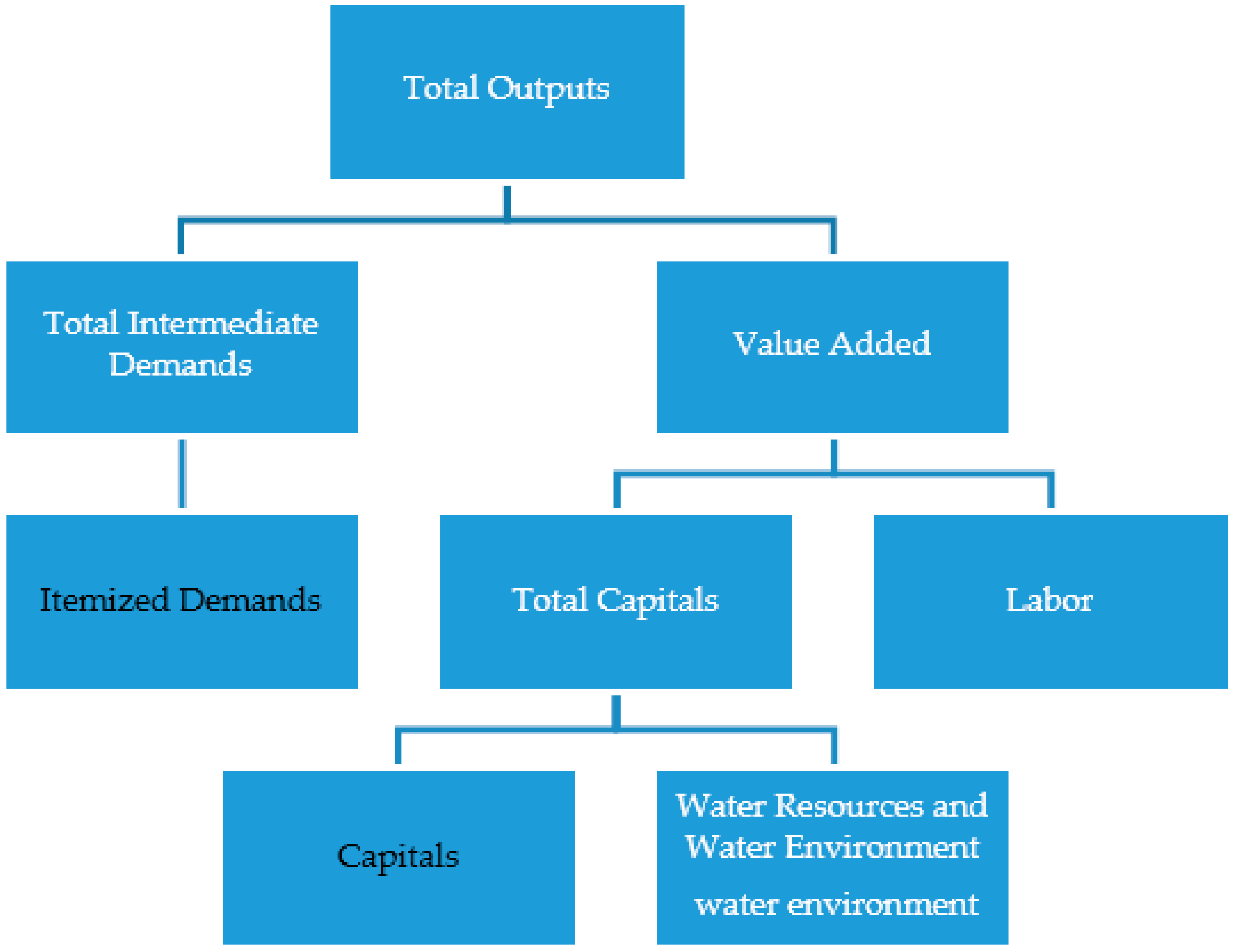
2.3. Extension of Traditional SAM

In view of water pollution and shortages which are caused by economic activities, water resources and water environment are built into the factors as part of the design of the WRWESAM. The novel accounts redesigned in the WRWESAM can be explained as follows.

1. Account of water pollution treatment sector (WPTS)

The function of this sector is to provide a service to meet environmental standards. The commodity of this sector is the value of the pollution cleanup and the activity is to remove pollution. In this study, the chemical oxygen demand (COD) removal amount is regarded as the pollution cleanup. Pollution cleanup may be viewed as special goods which are purchased at a certain price by polluters in order to reduce their pollution emission levels.

2. Account of water resources management sector (WRMS)

To investigate water resource utilization in production processes, WRMS was separated from the general production sectors. The commodity of this sector is the water for protecting water resources and the activity is to manage and protect water resources.

3. Account of water service of farming, forestry, animal husbandry and fishery (WSFFAHF)

In the WRWESAM, the commodity of this sector is the service for managing the irrigation water conveyance system of farming, forestry, animal husbandry and fishery, such as water control projects, reservoirs, sluices and canals. The activity of this sector is the corresponding management.

4. Account of water production and supply industry (WPSI)

According to the industrial classification standard for national economic activities in China, the commodity of WPSI is the water resources for national economic production activities while the activity is to produce and supply water resources.

5. The industrial sectors of the existing national economy in the SAM (AG, MI, MA, PSIEHG, SI)

In the WRWESAM, besides the aforementioned accounts, it does include all other industrial sectors. The commodities of these sectors are their production outputs and the activities are to produce these outputs.

6. Account of water resources and water environment factors (WRWE)

This account is a new virtual account of great importance and it accounts for the costs of resources and environment in the WRWESAM. As nature provides production activities with natural resources, such as indispensable resource stocks, i.e., land and minerals, environmental resources, i.e., water and air, nature should be charged with the environmental damage which is caused by weak governance of pollution treatment sectors and the emissions resulting from economic activities. WRWE in this study mainly refers to the water environmental rents and they are calculated by COD discharge amount as per the following formula:
Water environmental rents (RMB) = 0.7 (RMB/t) × COD discharge amount (t)

2.4. Description of the CGE Model

The CGE model is a general equilibrium model, capturing inter-sectoral interactions of the decision-making process in the economy. In order to get the optimization plans, the model includes producers and consumers, as well as government and foreign agents.
The CGE model is defined as a set of equations containing the equilibrium conditions to describe the relationships between supply and demand which formed the market. The mathematical equations of the model are presented in the Appendix A. There are seven kinds of modules in the CGE model, including COD discharge and COD removal, production, trade, final demand, commodity equilibrium (described in other modules), factor equilibrium and macro-closure modules.

1. COD discharge and COD removal module

(1) COD discharge
It is considered that there are closed relationships between the COD discharge amounts and the intermediate inputs, as well as the production outputs. Both COD discharging coefficients of intermediate inputs and production outputs may be regarded as unchanged.
(2) COD removal
The commodities of WPTS are identified as the COD removal amounts.

2. Production module

To distinguish the total capital and labor, a nested Constant Elasticity of Substitution (CES) production function was utilized to reflect the substitutes among various factors in the production process.
The total capital in the model include two parts (see Figure 1). One is capital which is assigned to residents and enterprises fairly, and the other one is water resources and the water environment which represents the water environmental rents. The impacts on the economy of Jiangsu province were simulated by increasing the discharge fees in different scenarios.

3. Trade module

Four parts are contained in the trade module, namely the product demand in the region, the product supply in the region, the call-in demand outside the region, as well as the callout supply outside the region.
The product demand in the region is defined by the normal Armington assumptions and divided into product demand in the region and call-in demand outside the region.
The direct quotation method is utilized to quote the prices or rates of exchange for different currencies in CGE model.

4. Final demand module

The residents’ demands, the government’s demands and other final demands are incorporated in the final demand module. The residents’ consumption is allocated to various commodities and service in the form of a linear expenditure system (LES). The demand equation in the LES can be written as Equation (A34) in Appendix A.4.1. Moreover, the total consumption of government comes from both local and central governments. Additionally, the fixed capital formation and the stock net change which have a consistent expenditure function forms are calculated in the final demands. In the nested structure of consumers’ final demands, the first layer reflects the demand for Armington commodity which is the sum of all activities in the economy.

5. Factor equilibrium module

The factor equilibrium contains labor, total capitals, as well as water resources and water environment equilibrium. The factor demands must equal the supplies in order to achieve the aim of factor market clearing.

6. Macro-closure module

The CGE model generally includes some equilibrium relationships between the residents’ revenue and expenditure, enterprises’ revenue and expenditure, government’s revenue and expenditure, as well as international revenue and expenditure.
The residents’ revenue and expenditure: The residents’ income consists of the factor income and the transfer payments from enterprises and local government. The residents’ consumption equals to residents’ after-tax income minus residents’ savings. The income should equal to the consumption.
Enterprises’ revenue and expenditure: The enterprises’ income should equal to the transfer payments to residents and government, plus the environmental rents.
Government’s revenue and expenditure: The local government’s income contains import tax, production valorem tax, individual income tax, enterprise direct tax and the financial amount from central government. The net savings of the local government should equal to the income minus the consumption of local government. The balance of the central government’s revenue and expenditure can be described as the local government.
Balance of international revenue and expenditure: The imports should equal to the exports.
The water environmental rent (Sn in Equation (A44)) represents as the fee which should have been paid to the nature by enterprises. The impacts of the discharge fees on the overall economy and each industry in Jiangsu province may be simulated and investigated by varying the values of Sn.

2.5. Parameter Determination

The CGE model of regional water resources and water environment contains several parameters, which are summarized as follows.

1. The parameters of CES function, CET function and Armington assumption

There is imperfect substitutability between labor and capital, domestic demands and imports, as well as incomplete conversion between domestic demands and exports by applying CES function, CET function and Armington assumption. More specifically, the elasticity values of substitution need to be inserted in CES function, CET function and Armington assumption in order to determine quantities and prices of various commodities and they can be obtained from literature or determined based on certain assumptions. The Generalized Maximum Entropy (GME) was applied to the parameter estimation of CES function, which emphasized the unknown parameters should be maximized under the constrained conditions [26]. Due to the difficulties of getting data for parameter estimation of CET function and Armington assumption, we have referred to certain assumptions from the Shanghai Academy of Social Sciences [27].
As WRMS and WPTS are separated from SI, and WSFFAHF is separated from AG, their elasticity values of substitution cannot be determined directly. Therefore, these elasticity values are replaced by the values before separation. The elasticity values of substitution of each sector are listed in Table 2.
The simultaneous equations are applied to represent CES function and CET function implicitly as:
Q = α [ δ x 1 ρ + ( 1 δ ) x 2 ρ ] 1 / ρ
p 1 p 2 = δ 1 δ ( x 2 x 1 ) 1 ρ
p q = p 1 x 1 + p 2 x 2
The share parameters and efficiency parameters may be solved as:
δ = x 1 1 ρ x 1 1 ρ + x 2 1 ρ
α = Q ( δ x 1 ρ + ( 1 δ ) x 2 ρ ) 1 ρ
where Q is the output, p i is the price, x i is the production input, p and q are the total price and total production inputs, δ and α are the share parameters and efficiency parameters, respectively.

2. The parameters of LES demand function

The consumers’ demand parameters and marginal budget shares have been obtained according to the consumption and price of commodities, disposable income of residents and expenditure elasticity calculated from the WRWESAM. The parameters of LES demand function are listed in Table 3.

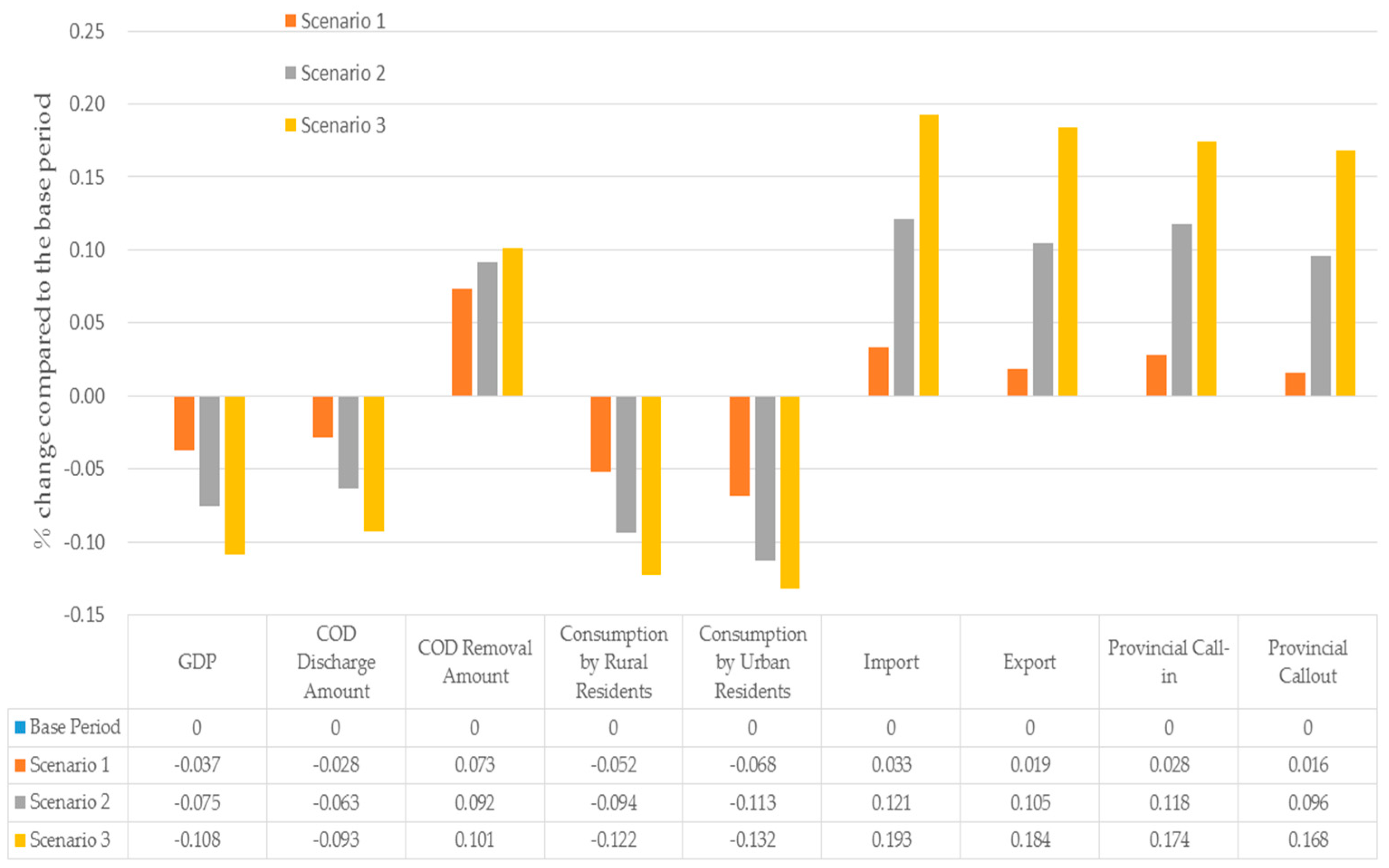
2.6. Simulating Impacts of the Discharge Fees

In the policy simulation, the correctness of the theory, the accuracy of the model and the integrity of the algorithm are quite important. A policy simulation model adopts the method of comparative static analysis which examines system changes from one balanced phase to another, taking no account of the switching process. In other words, the model only considers variance in the values of discharge fees.
An important virtual account—water resources and water environment factor—was incorporated into the extended WRWESAM, aiming to account for the unnoticeable costs for water pollution in traditional economic theories. This account is based on the costs which should have been paid to nature for water environment treatment by enterprises. In the model simulation, we defined an exogenous variable named Sn to express the water environmental rent and researched the impacts of various discharge fees by changing the values of Sn.
With water environmental rent incorporated into the CGE model, three scenarios are determined to estimate the possible effects of increases in discharge fees on regional economy. The discharge fee in 2012 was 0.7 yuan per ton. Here, we assumed that the government raised the discharge fee incrementally by 50% (scenario 1), 100% (scenario 2) and 150% (scenario 3). In addition, the prices of all commodities were assumed to be 1, the accuracy of the model could be examined through the quantities and prices.

3. Results and Discussion

3.1. Impacts on the Overall Economy

Adopting the CGE model of regional water resources and water environment, several policy indices are chosen to evaluate the impacts on the economy of Jiangsu province, namely GDP, COD discharge amount, COD removal amount, the consumption by rural and urban residents, the consumption of local and central government, capital formation, the stock change, imports and exports, as well as the provincial call-in and call-out. The simulation results are displayed in Figure 2. Also, it is noteworthy that there are almost no changes in the consumption of local and central government, the capital formation and the stock change, so they are invisible in Figure 2.
In general, the simulation results quantitatively demonstrate that the increases of discharge fees pose a negative impact on the economy of Jiangsu province. Compared with the base period, GDP in the three scenarios decrease by 0.037%, 0.075% and 0.108%, respectively. The fundamental reason is that the policy introduces a distortion in the market which prevents producers and consumers from maximizing all the market opportunities for trade. From this view, we may consider that the increases of discharge fees are disadvantageous to the macro economy of Jiangsu province.
Further, the consumption by rural and urban residents experiences the relative decreases while compared with the base period. The decline of the macro economy will lead to a decrease of residents’ incomes. As a result, their consumption capacities will drop proportionately.
In international trade, there is an obvious increase in the quantities of imports and exports, as well as the provincial call-in and call-out. As a response to the discharge fee policies, the enterprises will increase their purchasing power for obtaining advanced equipment from overseas in order to reduce wastewater and increase the foreign sales of their products to make profits. In consequence, it will stimulate the economic transactions to a certain extent.
However, the simulation results from the model also lead to some active impacts on the regional environment. As a response to the decrease of economic activities, COD discharge amount experiences a process of gradual decrease (0.028%, 0.063% and 0.093%) and the COD removal amount gradually increases (0.073%, 0.092% and 0.101%). The active impacts show us that the discharge fee policy is beneficial to the regional environment.

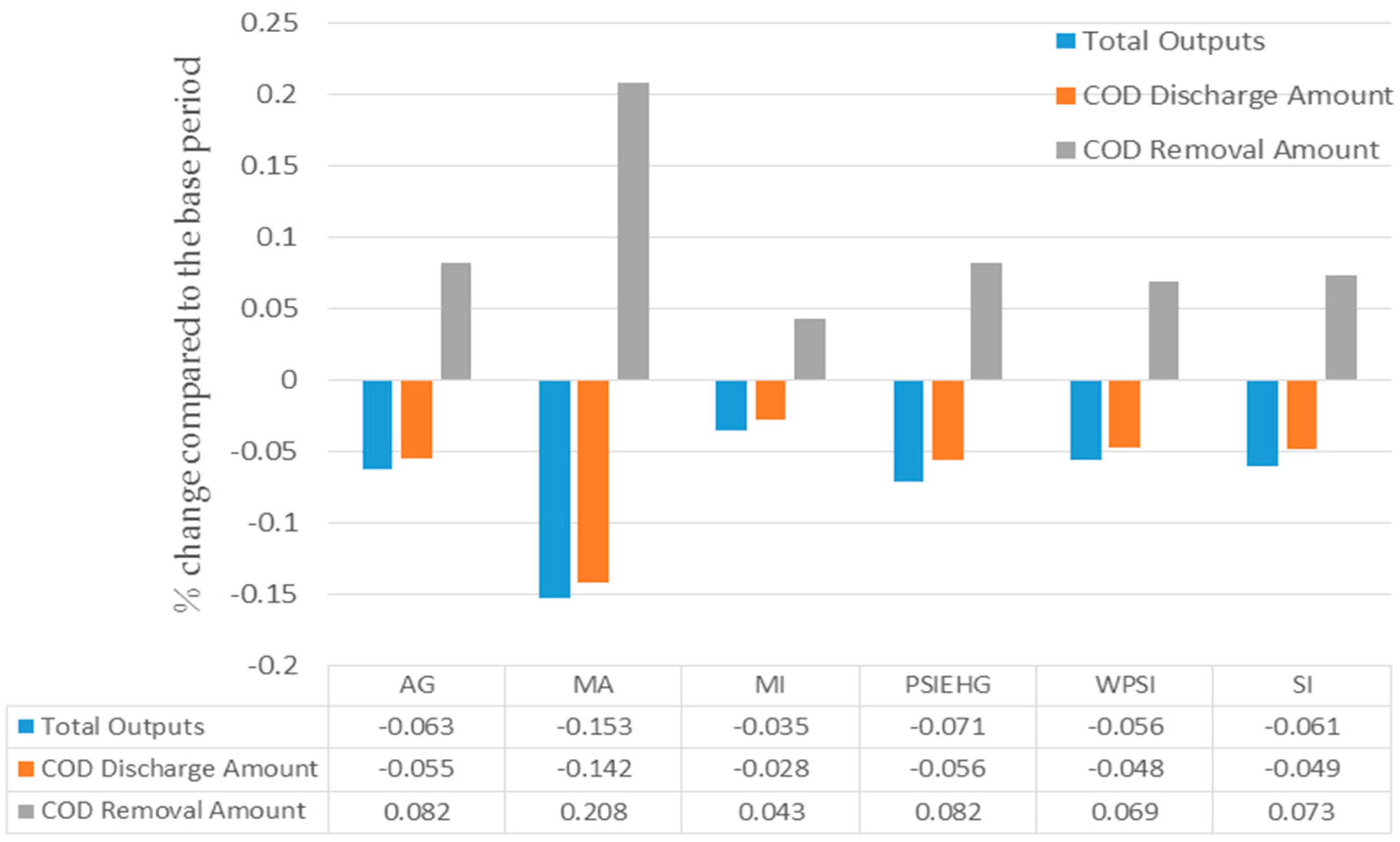
3.2. Impacts on Different Industries

The impacts on different industries of various discharge fees should be described by some indices, namely the total outputs, COD discharge amount and COD removal amount. We compared the three indices between scenario 2 and the base period.
As a result of Figure 3, the total outputs in different industries are decreased to different extents. The fundamental reason is that the increase of a discharge fee will downsize the enterprises’ production scales and, in consequence, the enterprises’ production outputs will be reduced synchronously. However, with the exception of MA, the total outputs of other industries drop. From Table 1 we can learn that MA has the largest share of production and they contribute the most to discharge in Jiangsu province. From the view of the economy, the industries with larger discharge are highly affected by the discharge fee policies and the proportion of their production outputs will drop.
Concerning the effectiveness of increasing the discharge fees on the regional environment, the simulation results also show the decrease in the amount of COD discharge and the increase in the amount of COD removal in different industries. The fundamental reason for this phenomenon is that the reduced economic activity would result in a lower discharge of COD. Moreover, with the policy implemented, the industries may increase their removal of pollution, aiming to meet environmental standards. For the industry with large discharge, such as MA, there are greater impacts on their COD discharge amount and COD removal amount. From the viewpoint of sustainability, this is beneficial for optimizing regional economic structures and regional environmental sustainability.

4. Conclusions

A CGE model of water resources and water environments was proposed to quantify the relationships among water resources, water environments and economic systems. The principles and methods relating to the environment and economy were employed to separate water resources and water environment sectors from the input and outputs source of the National Economic Production Department, aiming to take full account of the impacts of economic activities on water resources and water environments. The general equilibrium theory was employed to establish the CGE model, then the model parameters were quantitatively determined. Finally, the simulation results of impacts on the economy and water environment of Jiangsu province were obtained.
As a result, the increases in discharge fees would have negative impacts on the economy of Jiangsu province and lead to a decrease in GDP. The total outputs of each industry will be decreased to differing extents. Moreover, the industries with larger discharge are more greatly affected by the discharge fee policies and the policy will lead to an upgrade of the industrial structures from a situation of heavier pollution to one of lighter pollution. However, the policy is beneficial to the regional environment because of the reduction in COD discharge amounts and the increase in COD removal amounts. Overall, the discharge fee policy is beneficial to the sustainable development of the local economy and protection of the environment.

Acknowledgments

This work was funded by National Social Science Foundation of China (No. 2012 & ZD214), the Innovation Project of Graduate Student Training in Jiangsu Province (No. 1044/B14054) and the Priority Academic Program Development of Jiangsu Higher Education Institutions (PAPD).

Author Contributions

All authors made a substantial contribution to this manuscript. Guohua Fang and Ting Wang conceived and designed the methods and model; Xinyi Si collected and analyzed the data; Ting Wang and Xin Wen implemented the model and analyzed the results; Yu Liu prepared the manuscript and submitted it.

Conflicts of Interest

The authors declare no conflict of interest.

Appendix A

This appendix presents the equations of the CGE model.

Appendix A.1. COD Discharge and COD Removal Module

Appendix A.1.1. COD Discharge

COD discharge amount from intermediate inputs can be described as:
D C O D a = c Q I N T c a i d c c a
COD discharge amount from production outputs can be described as:
D C O D a = Q A a o d c a
The total COD discharge amount can be described as:
D C O D a = c Q I N T c a i d c c a + Q A a o d c a
where a is one of the nine sectors described in the WRWESAM, D C O D a is the total COD discharge amount of sector a, Q I N T c a and Q A a are the intermediate inputs of sector a for commodity c and the total outputs of sector a, i d c c a and o d c a , respectively, represent the COD discharging coefficients of intermediate inputs and production outputs.

Appendix A.1.2. COD Removal

The total COD removal amount can be described as:
R C O D a = c Q I N T c a i r c c a
where R C O D a is the total COD removal amount of sector a, i r c c a is the COD removal coefficient of intermediate inputs.

Appendix A.2. Production Module

Appendix A.2.1. The First Layer Nested

In the first layer, the composite total intermediate demands and value added are combined in the CES composite total outputs. Normally, the elasticity value of substitution is assumed to be zero, while the nested CES production function is regarded as a Leontief production function with the fixed coefficients. The Leontief (fixed coefficients) function is a special case of CES function when the elasticity value of substitution tends to be zero (σ→0) [13]. The nested Leontief-CES production function should be written as:
Q A a = α a q [ δ a q Q V A a ρ a + ( 1 δ a q ) Q I N T A a ρ a ] 1 ρ a , a A
P V A a ( 1 + τ g o v 1 , a + τ g o v 2 , a ) P I N V A a ( 1 + τ g o v 1 , a + τ g o v 2 , a ) = δ a q ( 1 δ a q ) ( Q I N T A a Q V A a ) 1 ρ a , a A
P A a Q A a = ( 1 + τ g o v 1 , a + τ g o v 2 , a ) P V A a Q V A a + ( 1 + τ g o v 1 , a + τ g o v 2 , a ) P I N T A a Q I N T A a , a A
where Q V A a and Q I N T A a are the value added and total intermediate demands, P A a , P V A a and P I N T A a are the prices of total outputs, value added and total intermediate demands. α a q is the efficiency parameter, δ a q and ( 1 δ a q ) , respectively, represent the shares of value added and total intermediate demands, ρ a is related to the elasticity value of substitution σ a = 1 / ( 1 ρ a ) , τ g o v 1 , a and τ g o v 2 , a , respectively, are the ad valorem taxes paid to the local and central governments.

Appendix A.2.2. The Second Layer Nested

There are two branches in the second layer. The first is the total intermediate demands which resolved into the various commodity demands of each industry.
Q I N T c a = i c a c a Q I N T A a , a A , c C
P I N T A a = c C i c a c a P Q c
where i c a c a represents the relationship between Q I N T A a and Q I N T c a , P Q c is the price of commodity c .
In the second branch, the total value added is decomposed into labor and total capital which contains the water resources and water environment factors.
Q V A a = α a v a [ δ l a v a Q L D a ρ a v a + ( 1 δ l a v a ) Q K D a ρ a v a ] 1 ρ a v a , a A
W L W K = δ L A v a ( 1 δ L A v a ) ( Q K D a Q L D a ) 1 ρ a v a , a A
P V A a Q V A a = W L Q L D a + W K Q K D a , a A
where Q L D a is the labor quantities, Q K D a is the rate of capital return of sector a , W L and W K are the prices of labor and capital respectively. α a v a is the efficiency parameter, δ l a v a and ( 1 δ l a v a ) are the share parameters, ρ a v a is the substitution parameter.

Appendix A.2.3. The Third Layer Nested

In the third layer, the composite total capital is decomposed into two parts: the various types of capital which include enterprises’ dividends, and households’ own capital, the water resources and water environment factors.
a Q K D a = Q K S
W K Q K S = k + S
where Q K S is the supplied total amount of capital, k is the sum of various capital, S is the water environmental rents which should have been paid to the nature and should be calculated from the related data in the water pollution treatment sector.

Appendix A.3. Trade Module

The commodities on the regional market are the goods, and the host organizations include residents and government. The substitution between the product supply in the region and the supply outside the region should be described by the Armington assumption:
Q Q c = α c q ( δ c q Q D C c ρ c q + ( 1 δ c q ) Q M c ρ c q ) 1 ρ c q , c C
P D C c P M c = δ c q ( 1 δ c q ) ( Q M c Q D C c ) 1 ρ c q , c C
P Q c = P D C c Q D C c Q Q c + P M c Q M c Q Q c , c C
where Q Q c , Q D C c and Q M c are the supplied commodity c in the whole market, in the domestic market, as well as outside the regional market. P Q c , P D C c and P M c are the prices of Q Q c , Q D C c and Q M c respectively. α c q is the efficiency parameter, δ c q is the share parameter and ρ c q is the substitution parameter.
The function of call-in outside the region is a Leontief production function, including the inter-regional call-in and import. Further, the import price is determined by the international market price, exchange rate and tariff, as seen in Equation (A18). The relationship should be written as:
Q M M r , a = i c a r , a Q M a , a A , r R
P M a = r R i c a r , a P M M r , a , a A , r R
P M M r o w , a = p w m r o w , a ( 1 + τ m a ) E X R , a A , r o w R
where Q M M r , a is the imports of sector a and the call-in products from other regions, P M M r , a is the price of Q M M r , a , i c a r , a is the relationship between Q M M r , a and Q M a , r o w means the foreign activities, p w m r o w , a is the commodity price which calculated with foreign currency (like dollars), τ m a is the customs tariff of the import commodity, E X R represents the exchange rate.
The total outputs in the region produce two kinds of “goods”, those for the markets in the region and those outside the region, which are aggregated by CET function. The quantity supplied is in the control of transform boundary and the producers will determine the quantity supplied of each market according to the relative price between various markets. The change of relative price between commodities in the region and outside the region has a great impact on the relative quantities, determined by the optimized first-order condition in Equation (A20). The simple form of CET function can be written as:
Q A c = α c t [ δ c t Q D A c ρ c t + ( 1 δ c t ) Q E c ρ c t ] 1 ρ c t , ρ c t 1 , c C
P D A c P E c = δ c t ( 1 δ c t ) ( Q E c Q D A c ) 1 ρ c t , c C
P A c = P D A c Q D A c Q A c + P E c Q E c Q A c , c C
where Q A c , Q D A c and Q E c are the total outputs in the region, commodity c for the domestic market and the provincial market. P A c , P D A c and P E c are the prices of Q A c , Q D A c and Q E c respectively. α c t is the efficiency parameter, δ c t is the share parameter and ρ c t is the transformation parameter which should be greater than 1.
The function of the call-out outside the region is a Leontief production function as well. It involves the inter-regional call-out and export, and the export price is determined by the international market price, as well as the export taxes and exchange rate, as seen in Equation (A26).
Q E E a r = i c a a r Q E a , a A , r R
P E a = r R i c a a r P E E a r , a A , r R
P E E a , r o w = p w e a , r o w ( 1 τ e a ) E X R , a A , r o w R
where Q E E a r is the exports of sector a and the call-out products to other regions, P E E a r is the price of Q E E a r , i c a a r is the relationship between Q E E a r and Q E a , p w e a , r o w is the FOB (free on board) price of commodities calculated with foreign currency, τ e a is zero in the WRWESAM.
P E E a e = p w e a E X R , a A , e R
Due to the one-to-one relationship between commodity and activity, there is a high coherence on the price and quantity of activities produced and sold in the region. The high coherence should be described as:
Q D C c = Q D A c , c C
P D C c = P D A c , c C
Q A c = a I D E N T a c Q A a , c C
P A c = a I D E N T a c P A a , c C
where I D E N T a c is the unit matrix.
Among them, the inter-regional call-in, the inter-regional call-out, the exchange rate, the FOB price and the commodity price which are calculated in foreign currency are all given exogenously. Then, the import and export prices may be obtained according to the above formulae.

Appendix A.4. Final Demand Module

Appendix A.4.1. The Residents’ Demands

The residents’ income consists of the factor income and the transfer payments from enterprises and local government. The residents’ consumption equals residents’ after-tax income minus residents’ savings.
Y H h = W L Q L S s h i f h , l + ( W K Q K S S ) s h i f h , k + t r a n s f r h , e n t + t r a n s f r h , g o v 1
Y D h = ( 1 t i g o v 1 , h t i g o v 2 , h ) Y H h Y h g
where Y H h , Y D h and Y h g are the incomes, consumptions and savings of the residents, respectively. Q L S and Q K S are the total quantities of labor and total capital, respectively, s h i f h , l and s h i f h , k are the share parameters of labor and capital, t r a n s f r h , e n t and t r a n s f r h , g o v 1 are the transfer payments from enterprises and local government, t i g o v 1 , h and t i g o v 2 , h are the income tax rates from residents to local and central governments, respectively.
The minimum living allowance and the actual additional income are the main parts of the residents’ demands.
Q H c , h = θ c , h + u c , h P A c ( Y D h c P A c θ c , h )
where Q H c , h is the residents’ demand for commodity c , θ c , h and u c , h are the consumers’ demand parameters.

Appendix A.4.2. The Government’s Demands

The total consumption of government comes from both local and central governments and the consumption quantities of commodities are all given exogenously.
E G g o v 1 = c P Q c Q G c , g o v 1 ¯ + h t r a n s f r h , g o v 1 + t r a n s f r g o v 2 , g o v 1
E G g o v 2 = c P Q c Q G c , g o v 2 ¯ + t r a n s f r g o v 1 , g o v 2
where E G g o v 1 and E G g o v 2 are the consumptions of local and central governments. Q G c , g o v 1 ¯ and Q G c , g o v 2 ¯ represent as the consumption quantities of local government and central government for commodity c respectively. t r a n s f r g o v 1 , g o v 2 and t r a n s f r g o v 2 , g o v 1 are the financial amount from local government to central government and the relationship reversed, respectively.

Appendix A.4.3. The Other Final Demands

The fixed capital formation and the stock net change are included in the final demands of other regions, which both given exogenously and should be written as:
E I N V = c P Q c Q I N V c ¯ , c C
S A V = c P Q c Q S A V c ¯ , c C
where Q I N V c ¯ is the investments of sector c , Q S A V c ¯ is the increase in stocks which including the deprecation, E I N V and S A V are the total fixed capital formation and the stock net change.

Appendix A.5. Factor Equilibrium Module

The equations should be written as:
a Q L D a = Q L S
a Q K D a = Q K S
Q L S = Q L S ¯
Q K S = Q K S ¯
W K Q K S = k + S
where Q L S and Q K S are the supplied total amount of labor and capital, Q L S ¯ and Q K S ¯ are the endowments of labor and capital, k is the total capital.

Appendix A.6. Macro-Closure Module

Y E N T = ( W K Q K S S ) s h i f e n t , k + S n
E N T S A V = Y E N T s e n t
t r a n s f r h , e n t = Y E N T ( 1 s e n t ) φ h , e n t
T R g o v 1 , e n t = Y E N T ( 1 s e n t ) φ g o v 1 , e n t
T R g o v 2 , e n t = Y E N T ( 1 s e n t ) φ g o v 2 , e n t
where Y E N T and E N T S A V are the incomes and savings of enterprises, s h i f e n t , k is the share parameter to enterprises, S n is the simulated discharge fee (as a exogenous variable ), s e n t is the share parameter of enterprises’ savings, t r a n s f r h , e n t is the transfer payments from enterprises to residents, T R g o v 1 , e n t and T R g o v 2 , e n t are the enterprises’ direct taxes for local and central governments, respectively. φ h , e n t , φ g o v 1 , e n t and φ g o v 2 , e n t are the distribution coefficients.
The closure of government revenue and expenditure involves the macro-closure of local and central governments. Moreover, the import tax, production valorem tax, individual income tax and enterprise direct tax are included in the government revenue and expenditure.
The balance of local government revenue and expenditure should be written as:
Y G g o v 1 = c p w m c τ m c Q M M r o w , c + a P A a Q A a τ g o v 1 , a 1 + τ g o v 1 , a + τ g o v 2 , a + h t i g o v 1 , h Y H h + T R g o v 1 , e n t + t r a n s f r g o v 1 , g o v 2 , a A , h H
where Y G g o v 1 is the total income of local government.
The balance of fiscal revenue and expenditure is not included in the model.
G S A V g o v 1 = Y G g o v 1 E G g o v 1
where G S A V g o v 1 is the local government net savings.
The balance of central government revenue and expenditure should be written as:
Y G g o v 2 = a P A a Q A a τ g o v 2 , a 1 + τ g o v , a + τ g o v 2 , a + h t i g o v 2 , h Y H h + T R g o v 2 , e n t + t r a n s f r g o v 2 , g o v 1 , a A , h H
where Y G g o v 2 is the total income of local government.
The same to local government, the gap between revenue and expenditure of the central government is regarded as the government net savings which is given endogenously.
G S A V g o v 2 = Y G g o v 2 E G g o v 2
where G S A V g o v 2 is the net savings of local government.
According to the system equilibrium conditions, all supplies should equal to demands in the region which should be written as:
Q Q c = a Q I N T c , a + h Q H c , h + Q G c , g o v 1 ¯ + Q G c , g o v 2 ¯ + Q I N V c ¯ + Q S A V c ¯ , c C
In this model, there is only regular import-export trade between the domestic and foreign accounts. The balance of international revenue and expenditure should be written as:
c p w m c Q M M r o w , c + F S A V = c p w e c Q E E c , r o w
c P M M p r o , c Q M M p r o , c + P S A V = c P E E c , p r o Q E E c , p r o
E X R = E X R ¯
where F S A V is the foreign savings, P S A V is the savings outside the region.
The open CGE model with water resources and water environment factor consists of Equations (A1)–(A56), among which the endogenous variables are as follows: i d c c a , o d c a , i r c c a , Q A a , Q V A a , Q I N T A a , P A a , P V A a , P I N T A a , Q I N T c , a , Q L D a , Q K D a , W L , W K , P Q c , Q Q c , Q D C c , Q M c , P D C c , P M c , Q M M r , c , P M M r , c , E X R , Q A c , Q D A c , Q E c , P D A c , P E c , P A c , Q E E c , r , P E E c , r , Y H h , Y D h , Q H c , h , E G g o v 1 , E G g o v 2 , E I N T , S A V , Q L S , Q K S , Y E N T , E N T S A V , t r a n s f r h , e n t , T R g o v 1 , e n t , T R g o v 2 , e n t , Y G g o v 1 , G S A V g o v 1 , Y G g o v 2 , G S A V g o v 2 , P S A V , F S A V and k , totaling 52 endogenous variables. There are 56 equations, among which Equation (A13) equals to Equation (A40), Equation (A14) equals to Equation (A43), Equation (A26) equals to Equation (A27), so the latter can be removed. The unique solution of this model may be determined according to the 53 equations.
The equation of investments-savings should be added with the foreign net savings on the right. Due to its redundancy in math, it is necessary to add the dummy variable VBIS which should be zero if the model is valid. Value added to GDP by agriculture (%) has been applied as one of the indexes to study agricultural water management in Asia and Oceania during the past decades and it played an important role in formulating policy suggestions [28,29,30]. Also, GDP growth results in an increase of indirect water productivity in the manufacturing blocks energy and water as well as service blocks [31]. In this paper, GDP should be analyzed to research the effects on the regional macro economy caused by policy change. Take the index as an endogenous variable and establish the equation as:
G D P = c h Q H c , h + c g Q G c , g + c Q I N V c + c Q S A V c + c r Q E E c , r r c Q M M r , c
All of the above Equations (A1)–(A57) completely constitute the regional water resources and water environment CGE model.

References

  1. Zhao, Y.; Wang, J.F. CGE Model and Application of Economic Analysis; China Economic Publishing House: Beijing, China, 2008. (In Chinese) [Google Scholar]
  2. Gao, Y. The development method and implementation review of environmental CGE model. Shanghai Environ. Sci. 2008, 27, 210–213. (In Chinese) [Google Scholar]
  3. Bergman, L. Energy policy modeling: A survey of general equilibrium approaches. J. Policy Model. 1998, 10, 377–399. [Google Scholar] [CrossRef]
  4. Piggot, J.; Walley, J.; Wigle, R. International Linkages and Carbon Reduction Initiatives. In The Greening of World Trade Issues; Anderson, K., Blackhurst, R., Eds.; The University of Michigan Press: Ann Arbor, MI, USA, 1992; pp. 29–115. [Google Scholar]
  5. Llop, M.; Ponce-Alifonso, X. Water and agriculture in mediterranean region: The search for a sustainable water policy strategy. Water 2016, 8, 66. [Google Scholar] [CrossRef]
  6. Robinson, S. Macroeconomics, financial variables and computable general equilibrium models. World Dev. 1991, 19, 1509–1525. [Google Scholar] [CrossRef]
  7. Nestor, D.V.; Pasurka, C.A. CGE model of pollution abatement process for assessing the economics effects of environmental policy. Econ. Model. 1994, 12, 53–59. [Google Scholar] [CrossRef]
  8. Seung, C.K.; Harris, T.R.; MacDiarmid, T.R. Economic impact of surface water reallocation policies: A comparison of supply-determined SAM and CGE models. J. Reg. Anal. Policy 1997, 27, 55–76. [Google Scholar]
  9. Seung, C.K.; Harris, T.R.; MacDiarmid, T.R. Economic impacts of water reallocation: A CGE analysis for walker river basin of Nevada and California. J. Reg. Anal. Policy 1998, 28, 13–34. [Google Scholar]
  10. Seung, C.K.; Harris, T.R.; Englin, J.E.Y.; Noelwah, R.N. Impacts of water reallocation: A combined computable general equilibrium and recreation demand model approach. Ann. Reg. Sci. 2000, 34, 473–487. [Google Scholar] [CrossRef]
  11. Robinson, S.; Gueneau, A. CGE-W: An Integrated Modeling Framework for Analyzing Water-Economy Links Applied to Pakistan. In Proceedings of the 16th Annual Conference on Global Economic Analysis, Shanghai, China, 12–14 June 2013.
  12. Decaluwé, B.; Patry, A.; Savard, L. When water is no longer heaven sent: Comparative pricing analysis in a CGE model. Cah. Trav. 1999, 99, 5. [Google Scholar]
  13. Decaluwé, B.; Patry, A.; Savard, L.; Thorbecke, E. Poverty Analysis within a General Equilibrium Framework; Working Paper 9909; African Economic Research Consortium: Nairobi, Kenya, 1999; pp. 3–43. [Google Scholar]
  14. Gómez, C.M.; Tirado, D.; Rey-Maquieira, J. Water exchanges versus water works: Insights from a computable general equilibrium model for the Balearic Islands. Water Resour. Res. 2004, 40, W10502. [Google Scholar] [CrossRef]
  15. Hatano, T.; Okuda, T. Water Resource Allocation In the Yellow River Basin, China Applying A CGE Model. In Proceedings of the Intermediate Input-Output Conference, Sendai, Japan, 26–28 July 2006.
  16. Cardenete, M.A.; Hewings, G.J.D. Water price and water reallocation in Andalusia: A computable general equilibrium approach. Environ. Econ. 2011, 2, 17–27. [Google Scholar]
  17. Watson, P.S.; Davies, S. Modeling the effects of population growth on water resources: A CGE analysis of the South Platte River Basin in Colorado. Ann. Reg. Sci. 2011, 46, 331–348. [Google Scholar] [CrossRef]
  18. Qin, C.; Jia, Y.; Su, Z.; Bressers, H.T.A.; Wang, H. The economic impact of water tax charges in China: A static computable general equilibrium analysis. Water Int. 2012, 37, 279–292. [Google Scholar] [CrossRef]
  19. Boccanfuso, D.; Estache, A.; Savard, L. A Poverty Inequality Assessment of Liberalization of Water Utility in Senegal: A Macro-Micro Analysis, Cahier de Recherché/Working Paper; unpublished work. 2005.
  20. Letsoalo, A.; Blignaut, J.; de Wet, T.; de Wit, M.; Hess, S.; Tol, R.S.J.; Van Heerden, J. Triple dividends of water consumption charges in South Africa. Water Resour. Res. 2007, 43. [Google Scholar] [CrossRef]
  21. Luckmann, J.; Grethe, H.; McDonald, S.; Orlov, A.; Siddig, K. An integrated economic model of multiple types and uses of water. Water Resour. Res. 2014, 50, 3875–3892. [Google Scholar] [CrossRef]
  22. Environmental Protection Department of Jiangsu Province. Available online: http://www.jshb.gov.cn/jshbw/hbzl/ndhjzkgb/201306/t20130605_236653.html (accessed on 5 June 2013). (In Chinese)
  23. Jiangsu Provincial Bureau of Statistics. 2012 Input-Output Table of Jiangsu; Jiangsu Provincial Bureau of Statistics: Nanjing, China, 2012. [Google Scholar]
  24. Jiangsu Provincial Bureau of Statistics. 2013. Available online: http://www.jssb.gov.cn/2013nj/indexc.htm (accessed on 20 April 2015). (In Chinese)
  25. Major Targets for National Economic and Social Development of Jiangsu Province. 2012. Available online: http://www.jssb.gov.cn/tjxxgk/tjsj/ndsj/201504/t20150420_259211.html (accessed on 20 April 2015). (In Chinese)
  26. Huo, Y.B. The Study on CSI Model Constructing & GME Integration Evaluating of Its Parameter. Ph.D. Thesis, Nanjing University of Science & Technology, Nanjing, China, 9 September 2004. [Google Scholar]
  27. Wang, L. Armington Elasticity Estimation in the Main Industry in Our Country—Based on State-Space Model. Master’s Thesis, Shanghai Academy of Social Sciences, Shanghai, China, 2013. [Google Scholar]
  28. Valipour, M. Future of the area equipped for irrigation. Arch. Agron. Soil Sci. 2014, 60, 1641–1660. [Google Scholar] [CrossRef]
  29. Valipour, M. Future of agricultural water management in Africa. Arch. Agron. Soil Sci. 2015, 61, 907–927. [Google Scholar] [CrossRef]
  30. Valipour, M. A comprehensive study on irrigation management in Asia and Oceania. Arch. Agron. Soil Sci. 2015, 61, 1247–1271. [Google Scholar] [CrossRef]
  31. Pérez Blanco, C.D.; Thaler, T. An input-output assessment of water productivity in the Castile and León Region (Spain). Water 2014, 6, 929–944. [Google Scholar] [CrossRef]
Figure 1. Nested relationships of production.
Water 08 00413 g001
Figure 2. The overall economic impacts of increases in discharge fees.
Water 08 00413 g002
Figure 3. The impacts on different industries from increases in discharge fees.
Water 08 00413 g003
Table 1. Water Resources and Water Environment Social Accounting Matrix (WRWESAM) of Jiangsu province 2012.
Unit: 100 Million Yuan RMBCommodityActivity
WRMSAGWSFFAHFMIMAPSIEHGWPSISIWPTSWRMS
CommodityWRMS 0
AG 0.01
WSFFAHF 0
MI 0.05
MA 1.07
PSIEHG 0.16
WPSI 0.01
SI 1.53
WPTS 0
ActivityWRMS6.04500000000
AG02992.780000000
WSFFAHF0071.94000000
MI000419.5600000
MA000056951.330000
PSIEHG000002295.02000
WPSI00000061.9100
SI000000020728.220
WPTS0000000022.89
FactorLabor 1.36
Capital 1.82
WRWE 0
ResidentRural
Urban
Enterprise
GovernmentLocal0104.820186.741498.220035.91 0
Central 0.03
Abroad 0593.960911.737314.8300203.48
Other Regions 0369.1701689.157756.57263.7901280.42
FCF
SNC
Unit: 100 Million Yuan RMBActivityFactor
AGWSFFAHFMIMAPSIEHGWPSISIWPTSLaborCapitalWRWE
CommodityWRMS02.660003.3900
AG296.889.711.392107.750.050205.820.24
WSFFAHF71.940000000
MI2.000.0538.012654.2234.810.2194.310.17
MA656.9111.01124.0133308.1939.479.75574.846.10
PSIEHG10.110.7733.021308.3372.9310.79213.420.36
WPSI0.310.730.4829.152.541.2210.920.02
SI178.018.0754.394508.9223.298.07358.643.67
WPTS1.560.021.104.900.330.025.050.01
ActivityWRMS
AG
WSFFAHF
MI
MA
PSIEHG
WPSI
SI
WPTS
FactorLabor168.4837.6472.304123.8710.3512.70420.267.36
Capital88.621.9653.556076.5334.4611.90502.704.83
WRWE0.310.010.5966.653.780.045.140.02
ResidentRural 226.25164.05
Urban 798.37111.29
Enterprise 883.45126.15
GovernmentLocal0012.54534.3343.441.38789.840.01
Central0028.172228.4991.832.51789.330.13
Abroad
Other Regions
FCF 0
SNC
Unit: 100 Million Yuan RMBResidentEnterpriseGovernmentExportsProvincial CalloutCapital Account
RuralUrbanLocalCentralFCFSNC
CommodityWRMS00 000000
AG454.46523.02 30.108.5521.06329.1870.412.11
WSFFAHF00 000000
MI7.314.59 000.0149.5108.68
MA688.461867.80 00132.3811381.375377.1470.77
PSIEHG66.6999.85 00085.1900.89
WPSI4.3230.53 000007.67
SI855.622715.87 2523.63716.54249.07724.465849.0031.87
WPTS2.009.50 000000
ActivityWRMS
AG
WSFFAHF
MI
MA
PSIEHG
WPSI
SI
WPTS
FactorLabor
Capital
WRWE
ResidentRural 60.64
Urban 1896.71214.00
Enterprise
GovernmentLocal22.1988.76221.51 535.84
Central33.29133.14353.59130.13
Abroad
Other Regions
FCF 1829.275744.276511.701117.32253.265−448.45−1210.60
SNC 743.59
Table 2. The elasticity value of substitution of each sector.
Sector Para.WRMSAGWSFFAHFMIMAPSIEHGWPSISIWPTS
σ C E S 0.19070.32300.32300.18860.75730.32340.32340.19070.1907
σ C E T 333333333
σ A r m . 1.92.22.22.82.82.82.81.91.9
Notes: where σ is the elasticity value of substitution, ρ is related to σ and it can be calculated as ρ = 1 1 / σ .
Table 3. The parameters of linear expenditure system (LES) demand function ( θ c , h ) of each sector.
SectorRural ResidentsUrban Residents
Basic Demand (Million Yuan RMB)Marginal Budget ShareBasic Demand (Million Yuan RMB)Marginal Budget Share
WRMS0 0
AG6946.40.40726,390.70.109
WSFFAHF0 0
MI15.20.008390.30.0003
MA46,748.10.234135,267.10.216
PSIEHG571.90.0657819.90.009
WPSI194.10.0031481.90.002
SI58,779.30.283114,041.40.661
WPTS137.40.001398.90.002

