Integrating Artificial Neural Networks into the VIC Model for Rainfall-Runoff Modeling

Abstract

A hybrid rainfall-runoff model was developed in this study by integrating the variable infiltration capacity (VIC) model with artificial neural networks (ANNs). In the proposed model, the prediction interval of the ANN replaces separate, individual simulation (i.e., single simulation). The spatial heterogeneity of horizontal resolution, subgrid-scale features and their influence on the streamflow can be assessed according to the VIC model. In the routing module, instead of a simple linear superposition of the streamflow generated from each subbasin, ANNs facilitate nonlinear mappings of the streamflow produced from each subbasin into the total streamflow at the basin outlet. A total of three subbasins were delineated and calibrated independently via the VIC model; daily runoff errors were simulated for each subbasin, then corrected by an ANN bias-correction model. The initial streamflow and corrected runoff from the simulation for individual subbasins serve as inputs to the ANN routing model. The feasibility of this proposed method was confirmed according to the performance of its application to a case study on rainfall-runoff prediction in the Jinshajiang River Basin, the headwater area of the Yangtze River.

1. Introduction

The Jinshajiang River, the headwater area of China’s Yangtze River, is rife with hydropower resources that will be ready to put into use once the cascade power stations currently under construction in the area are complete. The cascade dams will be responsible for flood control, hydroelectricity generation and agricultural and industrial water consumption, so water resource planning, particularly accurate predictions of runoff, will be of substantial economic and social importance. Managing water resources effectively will also protect the lower Yangtze region from flood disasters.

The physically-based variable infiltration capacity (VIC) model [1,2] is a soil vegetation atmospheric transfer scheme that explicitly depicts the impact of spatial variability in infiltration, precipitation and vegetation on water fluxes throughout the landscape. A variety of updates to the original VIC model have made it capable of simulating quite complex hydrological processes. The newest version of the VIC model is comprised of three soil layers, which allow for explicitly depicting the interactions between the surface and groundwater [3]. The upper two soil layers, which generate the surface runoff, are characterized by the dynamic effects of precipitation on soil moisture; the lower soil layer, which determines the product of the base flow, represents the gradual variations in seasonal soil moisture with respect to the interaction between deeper soil water and subsurface flow. Subgrid-scale heterogeneity is also represented in regards to soil moisture storage, evaporation and runoff production [1,2,4,5,6,7]. In recent studies, the VIC model has been applied to several different scales of watersheds [8,9,10]. The VIC model has also been applied in several other research fields, for example to simulate streamflow ensembles [11], snowmelt [12], global flood events [13] and to conduct uncertainty analysis of climate data and model parameter sets [14]. Given the numerous applications and updates to the VIC model throughout its nearly twenty years of existence, the current version of the model is well suited to parameterizing various factors of the water budget process, including horizontal soil moisture distribution, evapotranspiration, infiltration capacity and subsurface flow heterogeneities. Booming populations and the excessive construction of dams, however, have left the traditional routing model unable to accurately reflect complex hydropower regulation schemes as the respective runoff of each subbasin is post-processed with a routing model via linear superimposition [15,16].

The artificial neural network (ANN) was designed to mimic biological neural processes to execute “brain-like” computations and is known as a powerful tool for modeling multidimensional nonlinear problems. ANNs can be applied to various aspects of the hydrologic modeling field, such as rainfall-runoff modeling [17,18], groundwater modeling [19,20], water quality assessment [21], regional flood frequency analysis and reservoir operations [22,23]. ANNs can also be utilized as bias-correction tools for multiple-source data [24,25]. Abramowitz et al. [26], for example, used ANNs to characterize, quantify and ultimately resolve systematic errors in a land surface model (LSM). Despite the attractive potential capability to map nonlinearity in rainfall runoff behavior, ANNs have been questioned for this purpose due to their lack of physically-realistic components or parameters [27,28]. In response, researchers have focused on integrating the ANN form with conceptual hydrological models as opposed to applying the ANN alone as a simple black-box model [29,30,31,32]. These hybrid models can yield highly accurate forecasts of dynamic processes, as the combination appropriately captures unknown and nonlinear components of the mechanistic model via the neural network [29].

In addition to the major criticism that ANNs lack physical mechanisms, other scholars have pointed out that ANN establishment is random in the underlying system; the results may fluctuate even with the same configuration [33]. There is currently a general consensus that single-point forecasts from the ANN model have finite value due to the variability of the outputs or uncertainty in the optimization procedure. To feasibly and effectively use modeling techniques to conduct water resource planning, it is necessary to construct a reasonable prediction band of the hydrologic variables to secure reliable information that accurately represents hydrological problems [34]. In this study, the primary focus was establishing an appropriate ANN prediction band to generate prediction ensembles and assess the uncertainty of ANN outputs.

The VIC model is useful for characterizing the spatial variability of infiltration, precipitation and vegetation; the ANN model is useful for nonlinear mapping. This paper presents a hybrid hydrology model comprised of a VIC model and an ANN routing model. In the proposed model, outflow processes including overland flow and groundwater in each subbasin are simulated by the VIC model. Next, each subbasin’s simulated daily runoff errors are corrected by an ANN bias-correction model. For runoff routing, the initial streamflow and simulated runoff corrected by the ANN are input to an ANN routing model. Finally, the flow inputs are routed by the ANN routing model to the outlet of the network forming a hydrograph of the simulation.

2. Integrating ANNs with the VIC Model

2.1. Variable Infiltration Capacity Model

The VIC model is a hydrologically-based, macroscale land surface model that represents the spatio-temporal subgrid-scale variability of precipitation, infiltration, runoff generation, evaporation and vegetation. The outflow processes include quick runoff and slow runoff. Quick runoff includes saturation and infiltration excess runoff [35]; the ARNO model [36] represents the slow runoff. Rainfall, maximum and minimum temperature, vegetation type and soil texture are the main input variables to the VIC model for conducting daily runoff simulation. The daily generated grid cell flow is routed to the edge of the grid cell based on the physical topology of the area to be modeled, then routed to the watershed outlet through the river networks (for a more detailed description of the VIC model, interested readers are advised to refer to Liang and Xie’s previous study [35]). In the present study, the spatial resolution of the VIC model was on a 10 km × 10 km grid with a 24-h time step.

2.2. Artificial Neural Networks

ANNs are mathematical and computational models designed to mimic, per their namesake, biological neural networks [37]. As shown in Figure 1, an integrated ANN structure includes an input layer, an output layer and at least one hidden layer with different quantities of neurons in each layer. The number of hidden nodes in a neural network is typically determined by trial-and-error. Determining connection weights and patterns of connections appropriately is also crucial. The most commonly-used ANN in the hydrology field is a feed-forward network with a back-propagation (BP) training algorithm [38,39]. The weights connecting each layer can be modified until the errors are minimized or the stopping criterion is met.

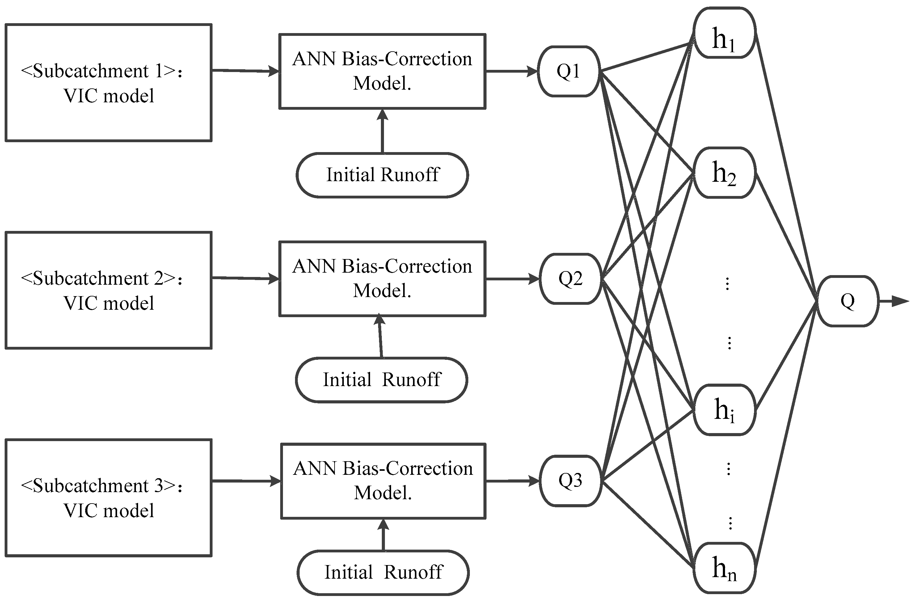
2.3. Hybrid VIC and ANN Model

The semi-distributed VIC model can explicitly represent the effects of the spatial variability of infiltration, precipitation and vegetation on water fluxes throughout the landscape. It cannot, however, accumulate the total runoff generated from individual subbasins by linear superposition alone. As discussed above, the hydrology model developed in this study was designed to integrate the advantages of both ANNs and the VIC model. A flow chart of the semi-distributed VIC model equipped with ANNs is provided in Figure 1. The hybrid model includes three components: The VIC model, the ANN bias-correction model (ABCM) and the ANN routing model (ARM). The first component simulates each subbasin runoff process by delineating and calibrating them separately. Next, each subbasin’s simulated daily runoff errors are corrected by the ABCM. The corrected streamflows from the simulation for the three subbasins are then input to the ARM, which routes them to the outlet of the network to form the hydrograph of the outlet of the entire watershed.

The VIC model can be driven by meteorological data and calibrated by streamflow data in each subbasin. To ensure the most accurate possible discharge is obtained, the simulated errors of the VIC model can be calculated using the initial streamflow and ABCM-simulated runoff using Equation (1):

$$E_i(t)=F_{{BP}_i}[Q_{{sm}_i}(t),Q_{{ob}_i}(t-1),Q_{{ob}_i}(t-2),\dots ,Q_{o{b}_i}(t-i)]$$

(1)

where $Q_{s{m}_i}(t)$ and $E_i(t)$ respectively denote the computed discharge and simulated error of each subbasin i at time t. $Q_{o{b}_{\mathrm{i}}}(t-1)$ denotes the initial flow of each subbasin i at time t − 1. $F_{BP}$ represents the BP neural network. It is necessary to test the autocorrelation of individual subbasin runoff values to obtain the ANN input parameters first, then the ANN can be used to establish the functional relationship of $Q_{o{b}_{\mathrm{i}}}\left(t\right)$ and $E_i(t)$. The ANNs in this model were designed for a “one-step-ahead” prediction, so there is a single node ($E_i(t)$) for the ANN output. Finally, the corrected flow $Q_{m{d}_i}(t)$ of each subbasin is calculated by adding $E_i(t)$ to $Q_{s{m}_i}(t)$:

$$Q_{m{d}_i}(t)=Q_{s{m}_i}(t)+E_i(t)$$

(2)

Typically, the initial subbasin flow affects the total runoff output during the concentration process. The total outflow $Q_{all}(t)$ at the whole basin outlet can be determined by inputting all subbasin-corrected flows using Equation (3), accordingly, where $Q_{all}(t)$ and $Q_{m{d}_i}(t)$ denote the total runoff output and corrected flow of each subbasin i at time t, respectively:

$$\begin{array}{ll}{Q}_{all}(t)=F_{BP}& [Q_{m{d}_1}(t),Q_{m{d}_1}(t-1),Q_{m{d}_1}(t-2),\mathrm{\dots },Q_{m{d}_1}(t-r),\\ & Q_{m{d}_2}(t),Q_{m{d}_2}(t-1),Q_{m{d}_2}(t-2),\mathrm{\dots },Q_{m{d}_2}(t-m),\\ & Q_{m{d}_{{}_3}}(t),Q_{m{d}_3}(t-1),Q_{m{d}_3}(t-2),\mathrm{\dots },Q_{m{d}_3}(t-n)]\end{array}$$

(3)

We used the shuffled complex evolution (SCE-UA) algorithm to optimize the VIC model for each subbasin. An ensemble of 100 models was acquired by training the ANNs 100 times with the SCE-UA algorithm. This arithmetic averaging technique was then applied to acquire the final output from the prediction band ensembles. Said technique is simple, effective and does not introduce any additional parameters as opposed to other approaches, like the principle of entropy maximization or weighted averaging. A cross-correlation approach was employed to secure reasonable input parameters [40,41]. Furthermore, the node quantity in the hidden layer of the ANNs was specified from one to 30 to optimize the ANN architectures.

3. Model Application and Case Study

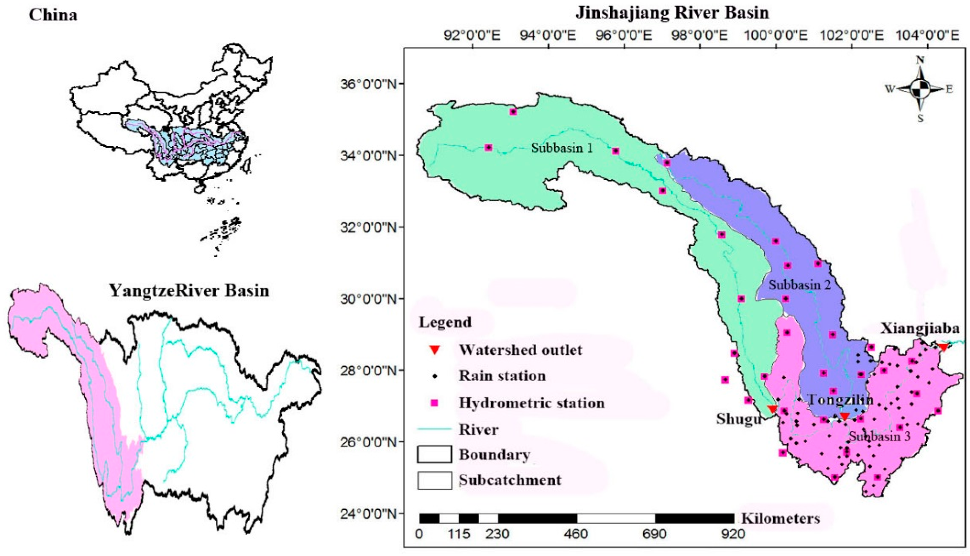
3.1. Study Area

The Jinshajiang River Basin, the headwater area of the Yangtze River, is mainly located in the east of the Tibetan plateau area. It has a drainage area of 326 × 10³ km², an annual average temperature from 16.4 °C to below zero and elevation ranging from 320 m to 6574 m. The area is characterized, as mentioned above, by an abundance of water resources. Precipitation in the basin gradually increases from northwest to southeast in a stepwise manner. Floods occur frequently during the five-month monsoon season from May to October. The whole basin can be delineated into three subbasins based on the underlying structure of the hybrid model, as shown in Figure 2. Subbasin 1, located upstream of the Jinshajiang River, is an area typically utilized for animal husbandry. Subbasin 2, which features especially abundant water resources, has been dammed by several cascade hydropower stations. The more populated downstream area, Subbasin 3, has also seen many large-scale water projects. To this effect, the discharge process in the area is likely influenced by anthropogenic activities (e.g., dams, irrigation and municipal water use) in addition to natural phenomena.

3.2. Data Preparation

Daily meteorological data including precipitation, maximum temperature and minimum temperature provided by the China Meteorology Administration were fed into the VIC model. One-hundred and ten precipitation observation stations provided daily precipitation data while maximum and minimum temperature information was provided by 33 meteorological stations (Figure 2). The inverse squared distance method was used to interpolate the daily climate variables to 10-km resolution. Soil texture in the Jinshajiang River Basin was classified according to the global Food and Agriculture Organization (FAO) soil maps with 10-km resolution (http://www.fao.org/geonetwork), and the vegetation dataset was derived based on Advanced Very High Resolution Radiometer (AVHRR) and land data assimilation system (LDAS) information. Land cover was defined by referring to the University of Maryland’s 14 types of global 1-km land cover data. Shuttle radar topography mission (SRTM) digital elevation data was downloaded from the SRTM website (http://www.cgiar-csi.org/data) with a spatial resolution of 3 arcs. Topography was obtained in ARCGIS software based on the digital elevation data.

3.3. Calibrating the VIC Model

Streamflow data measured between 2002 and 2010 for the three subbasins and total discharge records were used for the purposes of our case study. According to runoff measurements at the three hydrological control stations, the model was trained from 2003 to 2007 to capture both wet season and dry season information; it was validated for the period of 2008 to 2010. Warm-up data from 2002 were used to reduce sensitivity to state-value initialization errors. By inputting the meteorological data and observed streamflow data into the VIC model, the three subbasins were calibrated separately; the upstream monitoring station was calibrated first (including Subbasin 1 and Subbasin 2) followed by downstream Subbasin 3.

3.4. Configuring the ABCM

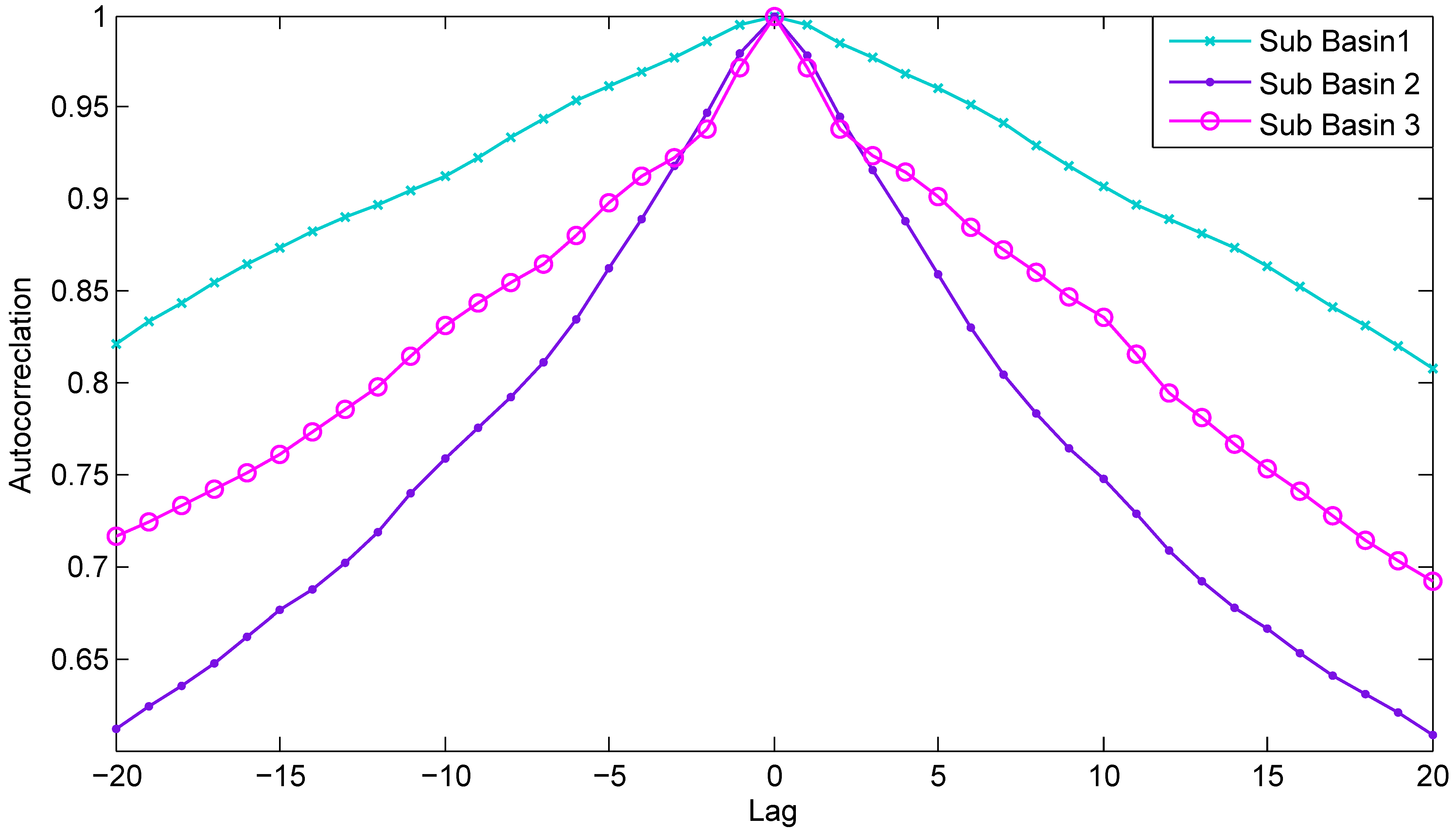
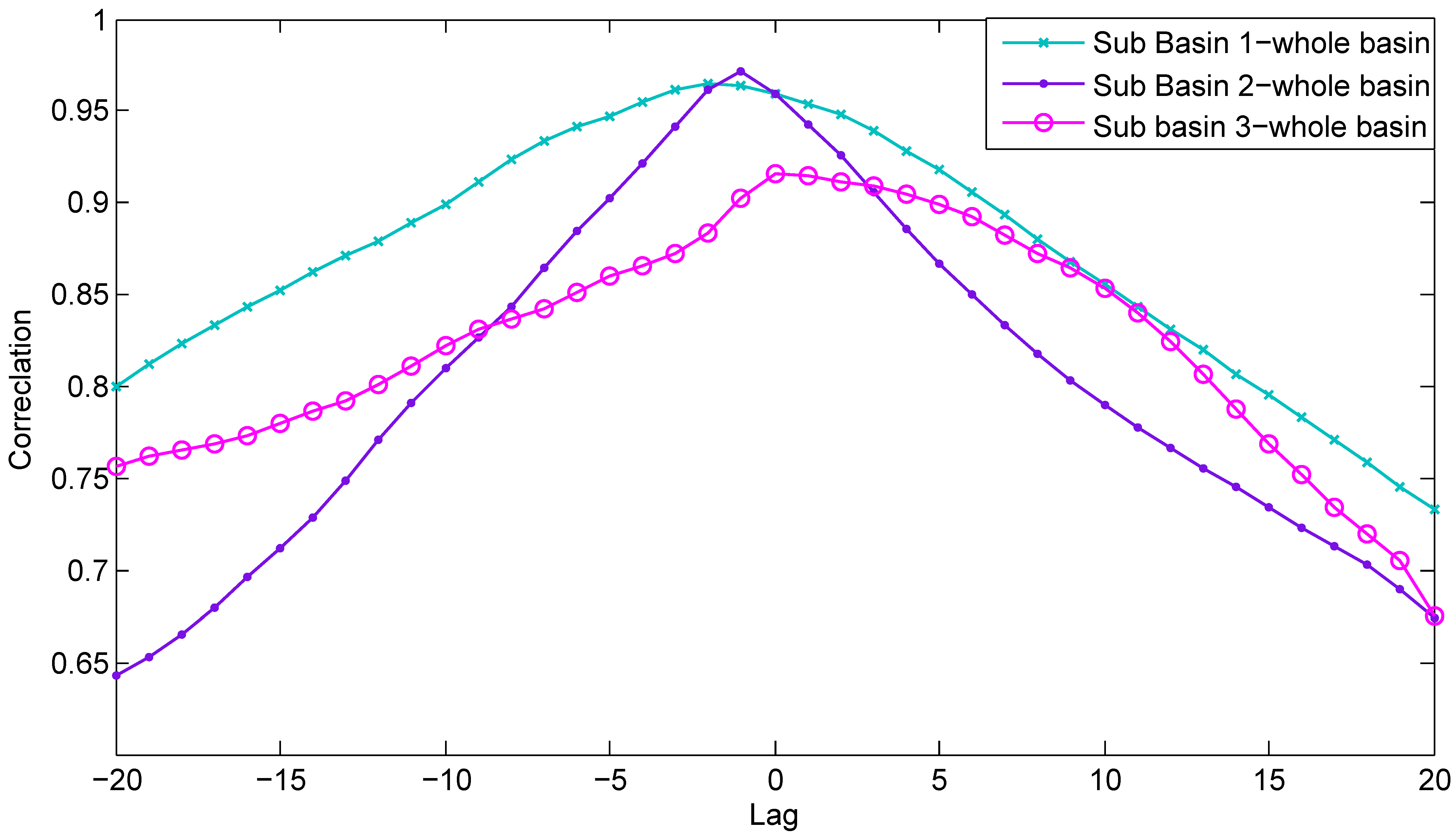
First, the appropriate input vectors of the ANN model were determined via auto-correlation among the dataset of each subbasin’s runoff (i.e., by statistical analysis). As shown in Figure 3, the correlation varied between the current streamflow and initial streamflow at different times in different basins. Any initial streamflow with a correlation coefficient larger than 90% plus the simulated streamflow at the current time were selected as the input vectors of each subbasin’s ABCM. This took place in a three-step process:

• Calculate $Q_{ob{s}_1}(t-1)$, $Q_{ob{s}_1}(t-2)$…, $Q_{ob{s}_1}(t-11)$ and $Q_{s{m}_1}\left(t\right)$ for Subbasin 1; $Q_{ob{s}_2}(t-1)$, $Q_{ob{s}_2}(t-2)$…, $Q_{ob{s}_2}(t-6)$ and $Q_{s{m}_2}\left(t\right)$ for Subbasin 2; $Q_{ob{s}_3}(t-1)$, $Q_{ob{s}_3}(t-2)$, $Q_{ob{s}_3}(t-3)$ and $Q_{s{m}_3}\left(t\right)$ for Subbasin 3.
• Let E_i(t) plus $Q_{s{m}_1}\left(t\right)$ be the corrected flow $Q_{m{d}_i}(t)$ of each subbasin.
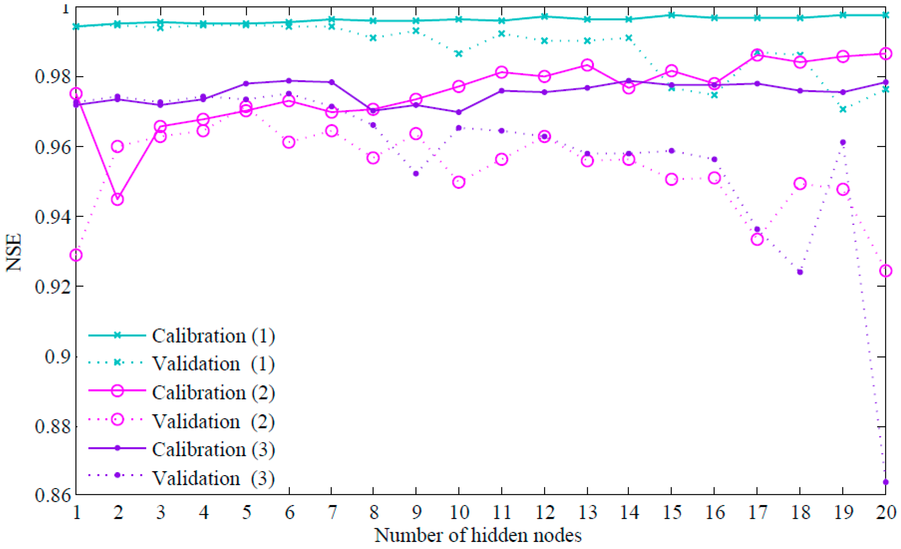
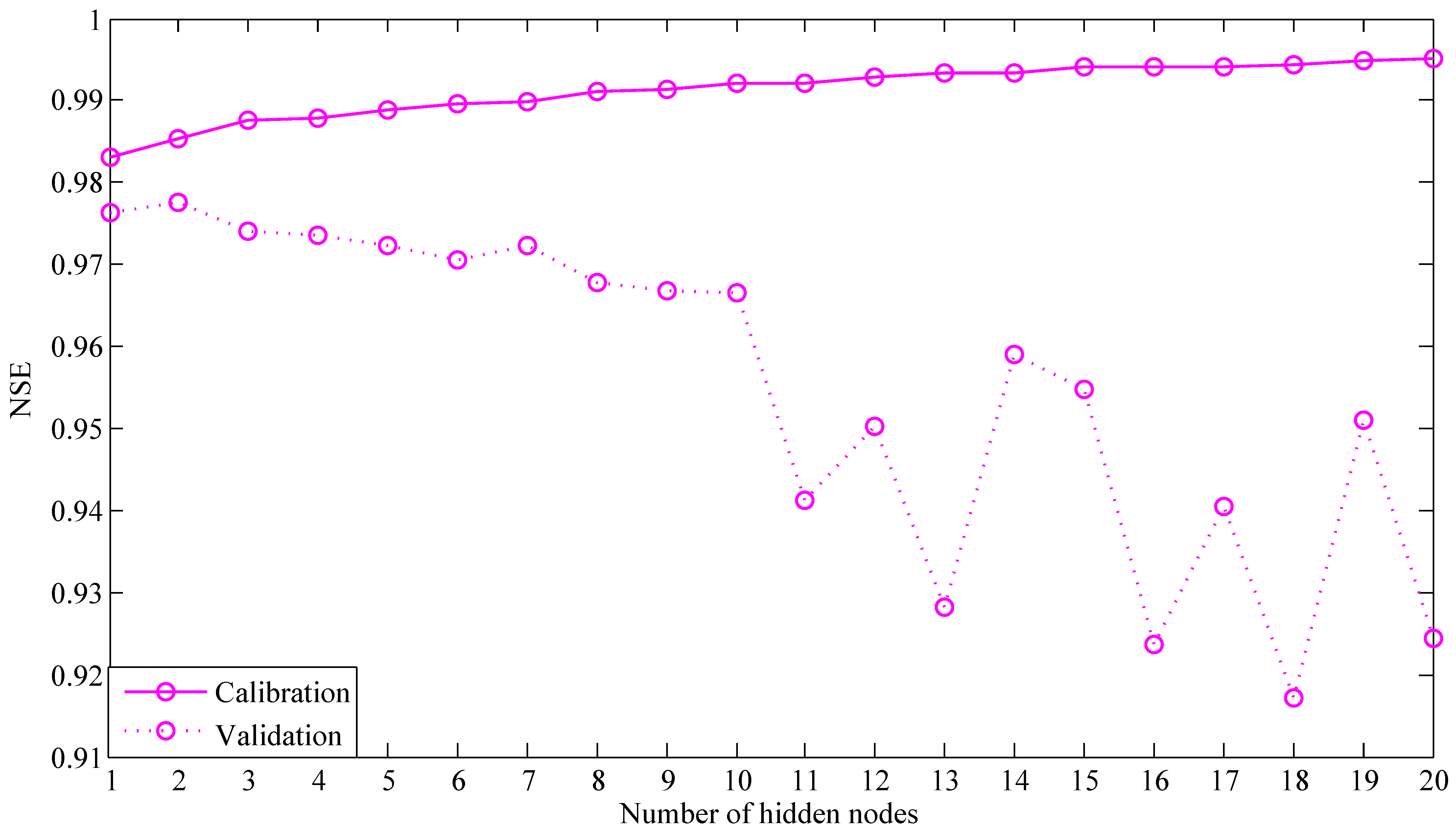
• Determine the optimal number of hidden neurons of each subbasin’s ABCM by trial-and-error.

Each ANN model was calibrated and validated 30 times independently and averaged to eliminate stochastic errors. To avoid over-training the ANNs, both the calibration and validation data were applied to search the optimal number of hidden neurons of each subbasin. The performance statistics of different hidden nodes of each subbasin’s ABCM in both calibration and validation periods are shown in Figure 4. As the number of hidden nodes increased, the Nash and Sutcliffe efficiency coefficient (NSE) value increased gradually in the calibration period; in the validation period, the NSE value first increased and then dramatically decreased. As a result, the subbasins’ ABCMs contained 4, 5 and 6 moderately hidden nodes, respectively.

3.5. Configuring the ARM

The ARM was established by inputting the corrected flow of every subbasin based on the correlation of subbasin runoff and total runoff (Figure 5). The performance of different hidden nodes of the ARMs in both calibration and validation periods are shown in Figure 6. Figure 5 and Figure 6 together indicate that the initial streamflow of subbasins that had correlation coefficients with current total runoff greater than 90% was successfully input into the ARM. This included calculating $Q_{m{d}_1}(t)$, $Q_{m{d}_1}(t-1)$…, $Q_{m{d}_1}(t-10)$ for Subbasin 1; $Q_{m{d}_2}(t)$, $Q_{m{d}_2}(t-1)$…, $Q_{m{d}_2}(t-5)$ for Subbasin 2; and $Q_{m{d}_3}(t)$, $Q_{m{d}_3}(t-1)$,$Q_{m{d}_3}(t-2)$ for Subbasin 3. The optimal quantity of hidden layer nodes was two.

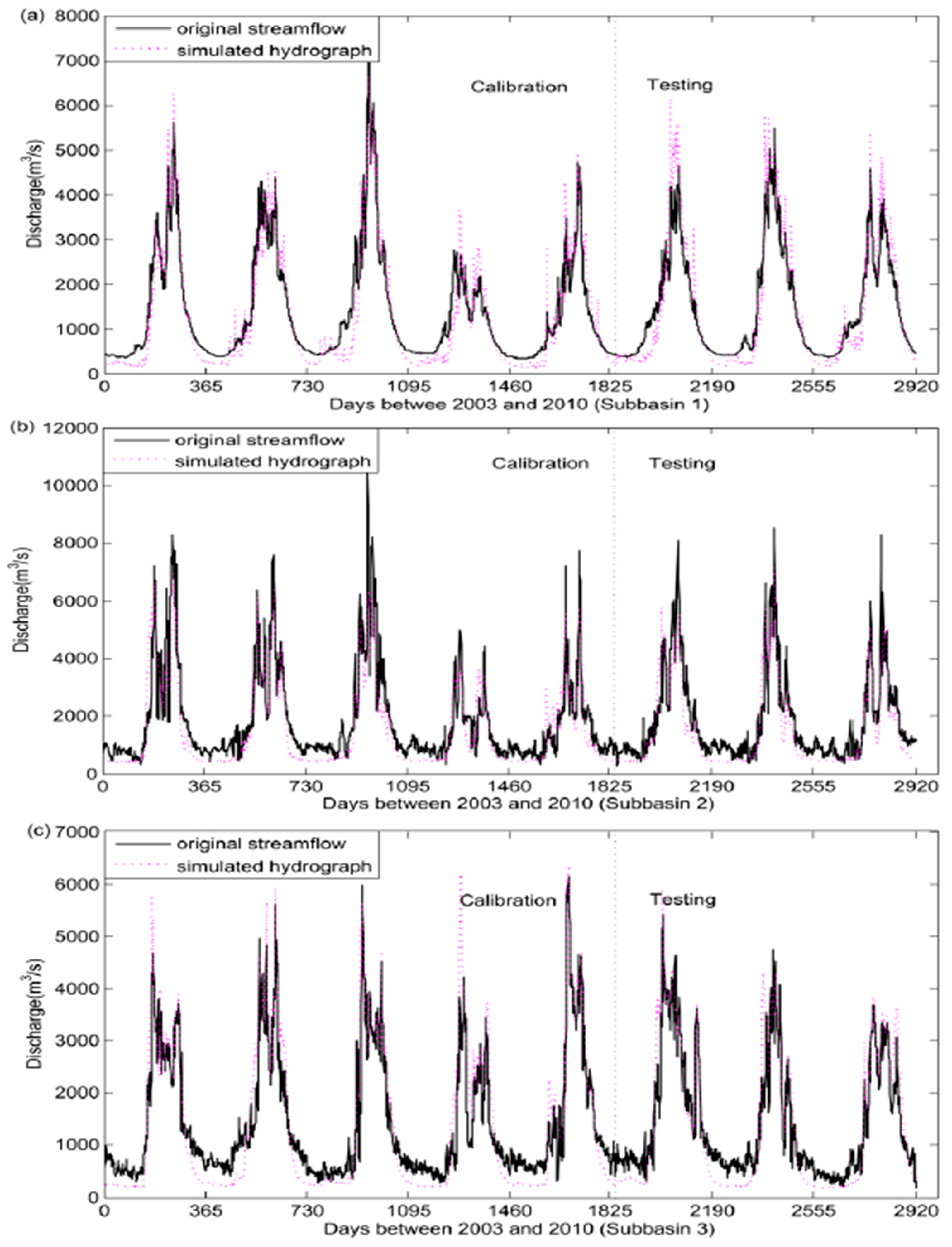
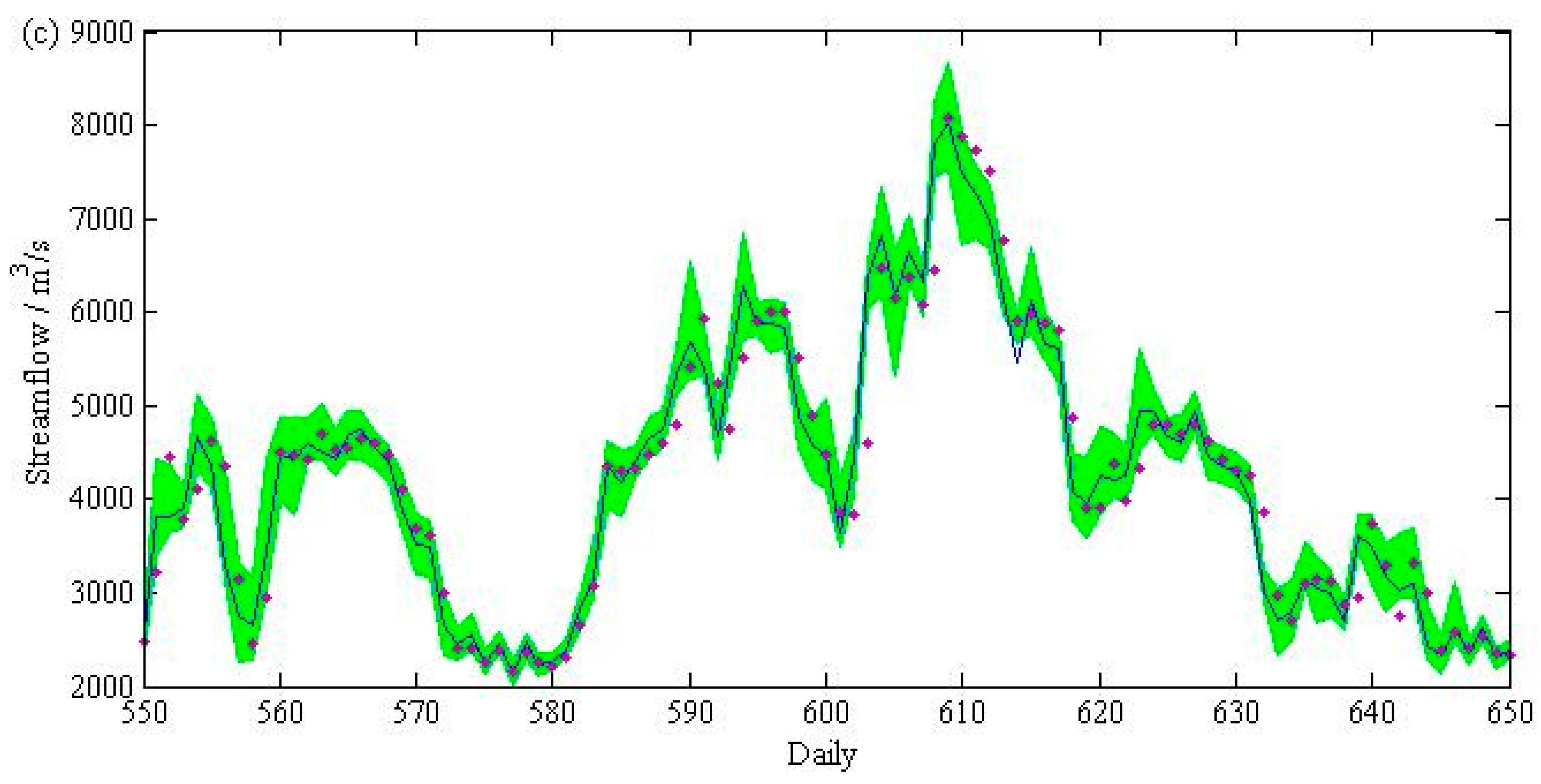
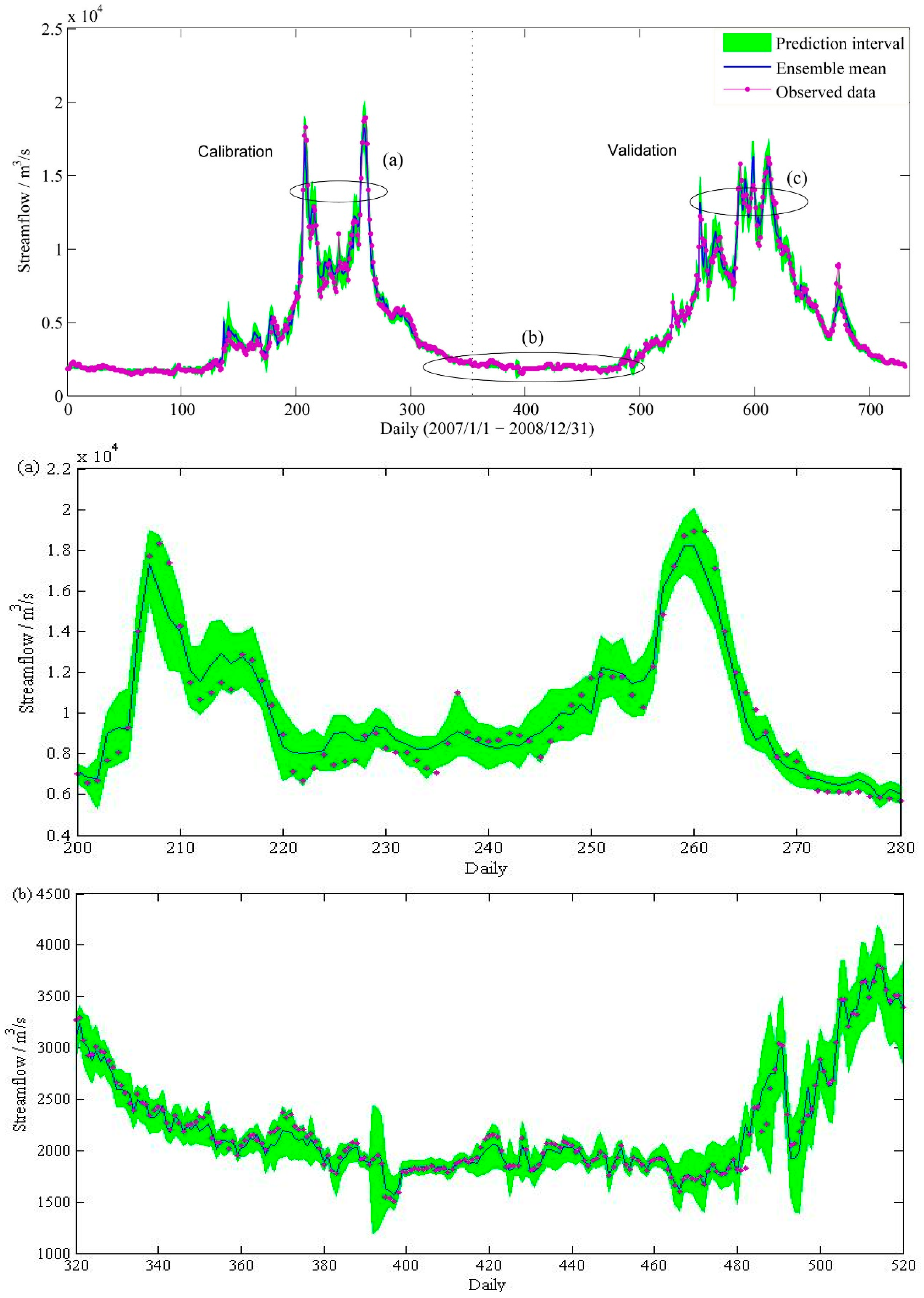
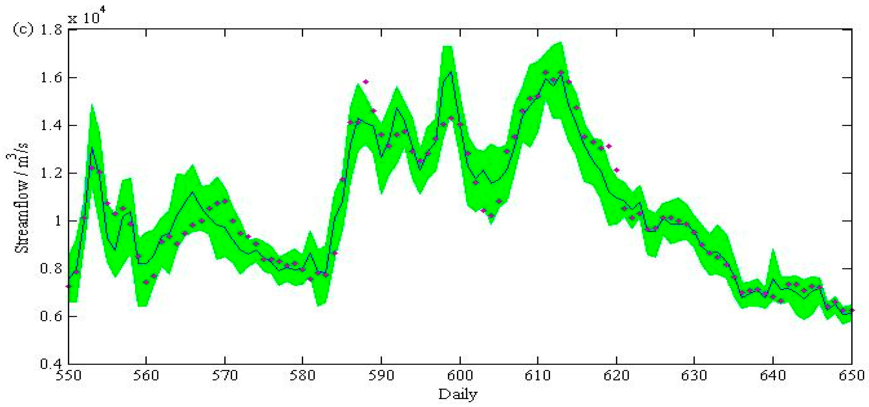
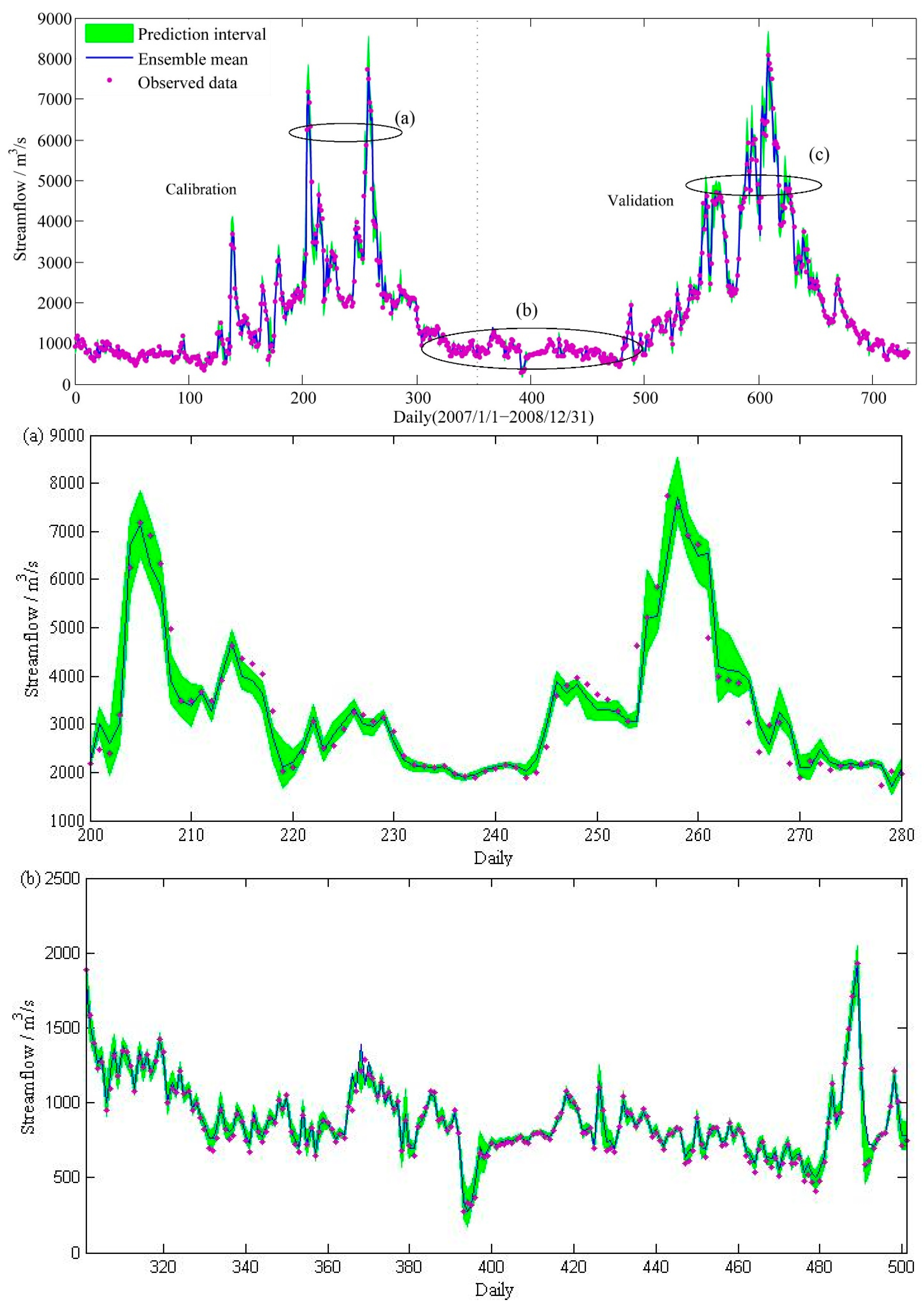
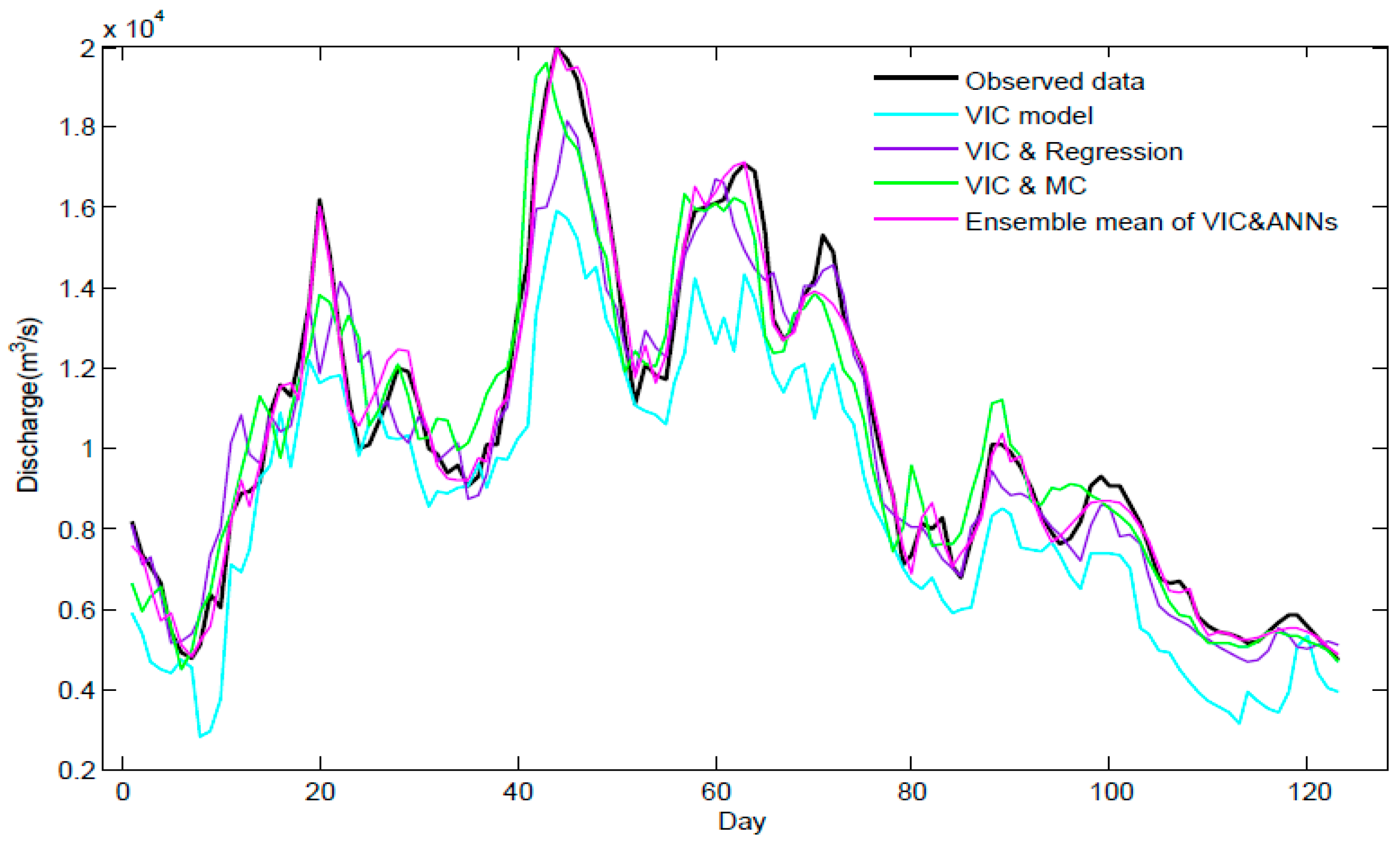
4. Results and Discussion

Table 1. Performance of the VIC model in each subbasin.

Model	Catchment	Calibration		Validation
		NSE	RE	NSE	RE
		(%)	(%)	(%)	(%)
VIC Model	Subbasin 1	86.63	8.73	85.39	1.34
	Subbasin 2	78.46	−18.61	78.23	−20.3
	Subbasin 3	78.82	−16.07	77.44	−16.57

reports the performance of the VIC model in each subbasin for both calibration and validation periods. Two statistical criteria were selected to assess the predictive capability of the hybrid model: the relative error (RE) and the NSE. Figure 7a–c display the time series of the measured and simulated streamflow of the three subbasins. As shown in Figure 7, the VIC model performance was indeed acceptable, and the simulated discharges were consistent with the observed streamflow series. Good NSE results were achieved for Subbasin 1, while Subbasins 2 and 3 had lower NSEs (Table 1).

Subbasin 1, located on the northeastern part of the Qinghai-Tibet Plateau, is upstream of the Jinshajiang River at the streamflow control station Shigu. Tableland and alpine valleys characterize the almost entirely undeveloped and steady flow above Shigu station. Conversely, the populated areas of Subbasin 2 and Subbasin 3 have experienced rapid development in recent decades, and thus, anthropogenic activities have remarkably altered the discharge process. In short, humans were likely responsible for the discrepancies among subbasins. The NSEs at the three subbasins exceeded 77%, and the RE values ranged between −20.3% and 1.34% in the calibration and validation periods. The streamflow was underestimated during all simulated periods, especially in the dry seasons, possibly due to the impact of operational reservoirs and relatively inadequate climate observation stations. These results were acceptable [43], but would need to be improved should they be applied to any actual engineering project.

The corrected ensemble mean flow of each subbasin was determined after bias-correction as shown in

Table 2. Performance measures for ABCM ensemble means.

Catchment	Calibration		Validation
	NSE	RE	NSE	RE
	(%)	(%)	(%)	(%)
Subbasin 1	99.76 (99.68–99.75)	0.09 (−0.04–0.11)	99.72 (99.65–99.73)	0.47 (0.08–0.62)
Subbasin 2	97.92 (96.81–98.24)	1.73 (1.35–2.23)	97.63 (96.19–98.87)	1.94 (1.25–3.12)
Subbasin 3	97.81 (96.29–98.23)	1.85 (1.07–2.14)	97.19 (95.82–96.64)	2.13 (2.34–3.97)

Note: Italicized values are the range of model performance across 100 ANN models. Ensemble means exceeding a single ABCM are bolded.

. By comparison between Table 1 and Table 2, the ABCM was found to reduce the RE and improve the NSE significantly during the calibration and validation periods. The consistently good performance over the calibration and validation periods suggests that the ABCM has favorable generalization properties and also rules out the possibility of preferable results being a result of overtraining the ANN model. The performance of Subbasin 1, which had an NSE value of approximately 100%, was quite a bit better than the other two subbasins (which had NSE values ranging from 97.19% to 97.92%). The RE values of the three subbasins were positive after being corrected by the ABCM, indicating that the model overestimated all simulated phases.

The daily ensemble prediction band of runoff for Subbasin 2, as well as its ensemble mean, observed values and VIC model-simulated values are shown in Figure 8. For the high flow, the forecasting width was wide, and thus, the coverage probability was high; the opposite was the case for the low flow. The forecasting width was slightly higher in the validation period than in the calibration period, and the ensemble mean was consistent with the observed data. In effect, the ABCM was able to correct errors in the VIC simulation and reproduce the seasonal hydrograph effectively in terms of both the magnitudes and timing of peak floods. Table 2 and Figure 8 together indicate that the ensemble consisting of independent ABCMs neutralized ensemble average errors; the resulting ensemble averages could serve as the final results for practical application. It is worth mentioning that some ensemble means exceeded some single ABCMs (bolded in Table 2).

The performance of the VIC and ANN ensemble mean model in terms of NSE and RE during the calibration and validation periods is presented in

Table 3. Traditional VIC model, VIC and ANN ensemble mean model, VIC and linear regression model and VIC and MC model performance during calibration and validation. MC, Muskingum-Cunge.

Model	Calibration		Validation
	NSE	RE	NSE	RE
	(%)	(%)	(%)	(%)
VIC	78.03	−21.51	78.47	−20.02
VIC and MC	95.77	−1.53	95.34	−0.85
VIC and Regression	95.62	−1.74	95.11	−1.2
VIC and ANN	98.89 (98.24–98.92)	0.43 (0.24–0.46)	97.76 (96.73–97.85)	−0.86 (−1.11–0.14)

, along with the performance of the VIC model using the traditional linear routing model. To further explore the potential of the proposed hybrid model, the output prediction results from the VIC and ANN ensemble mean model were compared against those of the VIC and linear regression model and the VIC and Muskingum–Cunge (MC) model. The linear regression model built a linear relationship between the streamflows of each subbasin based on the VIC model and the total runoff at the whole basin outlet. The MC method provided a numerical solution based on the traditional Muskingum routing model [44]. As a mesoscale river-routing scheme (RRS), the MC method has been coupled to land surface models (LSMs), such as the African Monsoon Multidisciplinary Analysis (AMMA) Land Surface Model Intercomparison Project, Phase 2 (ALMIP-2) [45].

The daily discharge behavior at the whole basin outlet was less accurately reproduced than that at any single subbasin outlet (Table 1 and Table 3). The integrated models drastically outperformed the traditional VIC model in both calibration and validation periods, as shown in Table 3. The traditional linear superposition routing method used in the VIC model cannot accurately represent the complex, dynamic runoff process. The evaluation indices of the VIC and linear regression model and the VIC and MC model were very similar, indicating that the two integrated models had comparable performance. Although the MC model has a comprehensive physical support, it is difficult to operate due to the large amount of data that it requires and the massive computational burden associated with it. The performance of the VIC and linear regression model was certainly inferior to the VIC and ANN ensemble mean model despite certain advantages (e.g., simplicity, facile implementation). Generally, the VIC and ANN ensemble mean model performed best; its NSE values ranged from 97.76% to 98.89%, and its RE values ranged between −0.86% and 0.43%. In short, the VIC and ANN model very accurately characterizes rainfall-runoff relationships. A comparison of the measured and predicted daily streamflow results from the traditional VIC model, VIC and ANN ensemble mean model, VIC and linear regression model and VIC and MC model is shown in Figure 9.

In order to evaluate the predictive uncertainty in different flow domains, the entire dataset was partitioned into three parts [46]: low flow (x ≤ μ (average value)), medium flow (μ < x < μ + 2δ (standard deviation)) and high flow (x ≥ μ + 2δ) [47]. The percentage of coverage (POC) and prediction interval with reference to ensemble average (PIEA) statistics of the VIC and ANN model at the whole basin in different runoff domains, along with the total dataset, are listed in

Table 4. Estimates of uncertainty indices in different flow domains for the VIC and ANN model (daily). POC, percentage of coverage.

Model Phase	Category	POC (%)	Prediction Band with Respect to Ensemble Mean (%)	No. of Patterns	% of Total Data
Calibration	Complete flow	64.45	8.74	1826	100
	Low flow	58.98	6.83	1213	66.40
	Medium flow	72.36	11.43	515	28.20
	High flow	90.63	12.03	98	5.39
Validation	Complete flow	66.92	10.89	1096	100
	Low flow	59.15	8.44	675	61.62
	Medium flow	76.95	12.08	338	30.86
	High flow	89.49	13.07	83	7.52

. The POC was 64.45% during the calibration period and 66.92% during the validation period for the total dataset. As the two indices of a higher coverage probability and narrower forecasting width are mutually exclusive, the PIEA was lower in the calibration period (8.74%) compared to the validation period (10.89%). These results suggested that the hybrid model is feasible and consistent.

The daily ensemble prediction band of runoff for the whole basin, as well as its ensemble mean, observed values and VIC model-simulated values are presented in Figure 10. Compared to Figure 8, the forecasting width of the whole basin was wider regardless of the period. The whole basin is very large, so the hydrological processes at work across it are highly complex and nonlinear; it is very challenging to represent all of the operational factors related to dams or agricultural activities in the area. That being said, these factors do have some regular patterns. For example: in the summer, individuals living in the area use more water for drinking, irrigation and filling reservoirs. The ANN model (especially the ANN ensemble mean) is a vital tool for seeking these patterns to improve the forecasting performance of the model on the whole.

5. Summary and Conclusions

An integrated rainfall-runoff model based on VIC and ANN models was built and implemented in the Jinshajiang River Basin in this study. The spatial distribution characteristics of the model input parameters were represented accurately by the VIC model considering the heterogeneity of the physico-geographical components, while the nonlinear mapping of runoff from each subbasin to the total streamflow at the whole basin outlet was established by two ANN models. Ensemble predictions were determined by constructing a prediction interval for the ANN models and then used to assess uncertainty and to improve the model’s reliability. The results of the case study indicated that the hybrid hydrology model based on the VIC and dual ANNs outperformed several other similar models and, further, that the proposed model can feasibly and effectively represent rainfall-runoff in areas like the Jinshajiang River Basin. The results of this study also may provide a scientific reference for basin-scale flood control, for better understanding the impact of climate change on streamflows and for conducting water resource management in the Jinshajiang River Basin and other regions with similar climatic characteristics (e.g., the Xin River Basin [48]).

This study was not without limitations. For example, limited data from only three stations were used to build the proposed model, and the soil data and vegetation data were assumed to be consistent on a yearly basis. The routing scheme used to simulate each subbasin is linear, which is disadvantageous in regards to generalizability. It is imperative to carefully account for hydrological blockages, like dams and certain anthropogenic activities in the watershed, as they considerably alter the hydrological regimes. Dam regulation schemes vary with various inflows, so in a future study, we will account for runoff classification and build three independent ABCMs and ARMs accordingly based on drought years, normal years and wet years. We plan to focus on taking runoff classification into account to improve the VIC model’s performance and to reduce model uncertainty, as well. We also hope to secure a greater quantity of measurements that can be used to further explore the modeling performance of increasing subdivision levels in the VIC model.

References

1. Liang, X. A simple hydrologically based model of land-surface water and energy fluxes for general-circulation models. J. Geophys. Res. 1994, 99, 14415–14428. [Google Scholar] [CrossRef]
2. Liang, X. Surface soil moisture parameterization of the VIC-2L model: Evaluation and modification. Glob. Planet. Chang. 1996, 13, 195–206. [Google Scholar] [CrossRef]
3. Liang, X.; Xie, Z.H.; Huang, M.Y. A new parameterization for surface and groundwater interactions and its impact on water budgets with the variable infiltration capacity (VIC) land surface model. J. Geophys. Res. 2003, 108. [Google Scholar] [CrossRef]
4. Nijssen, B.; Schnur, R.; Lettenmaier, D.P. Global retrospective estimation of soil moisture using the variable infiltration capacity land surface model, 1980–1993. J. Clim. 2001, 14, 1790–1808. [Google Scholar] [CrossRef]
5. Nijssen, B. Predicting the discharge of global rivers. J. Clim. 2001, 14, 3307–3323. [Google Scholar] [CrossRef]
6. You, Q.; Min, J.; Zhang, W.; Pepin, N.; Kang, S. Comparison of multiple datasets with gridded precipitation observations over the Tibetan Plateau. Clim. Dyn. 2015, 45, 791–806. [Google Scholar] [CrossRef]
7. You, Q.L.; Min, J.Z.; Kang, S.C.; Pepin, N. Poleward expansion of the tropical belt derived from upper tropospheric water vapour. Int. J. Climatol. 2015, 35, 2237–2242. [Google Scholar] [CrossRef] [Green Version]
8. Mo, K.C.; Lettenmaier, D.P. Hydrologic prediction over the conterminous United States using the national multi-model ensemble. J. Hydrometeorol. 2014, 15, 1457–1472. [Google Scholar] [CrossRef]
9. Park, D.; Markus, M. Analysis of a changing hydrologic flood regime using the Variable Infiltration Capacity model. J. Hydrol. 2014, 515, 267–280. [Google Scholar] [CrossRef]
10. Eum, H.I.; Dibike, Y.; Prowse, T.; Bonsal, B. Inter-comparison of high-resolution gridded climate data sets and their implication on hydrological model simulation over the Athabasca Watershed, Canada. Hydrol. Process. 2014, 28, 4250–4271. [Google Scholar]
11. Warrach-Sagi, K.; Wulfmeyer, V.; Grasselt, R.; Ament, F.; Simmer, C. Streamflow simulations reveal the impact of the soil parameterization. Meteorol. Z. 2008, 17, 751–762. [Google Scholar] [CrossRef]
12. Tan, A.; Adam, J.C.; Lettenmaier, D.P. Change in spring snowmelt timing in Eurasian Arctic rivers. J. Geophys. Res. 2011, 116. [Google Scholar] [CrossRef]
13. Wu, H.; Adler, R.F.; Tian, Y.; Huffman, G.J.; Li, H.; Wang, J. Real-time global flood estimation using satellite-based precipitation and a coupled land surface and routing model. Water Resour. Res. 2014, 50, 2693–2717. [Google Scholar] [CrossRef]
14. Eum, H.I.; Yonas, D.; Prowse, T. Uncertainty in modelling the hydrologic responses of a large watershed: A case study of the Athabasca river basin, Canada. Hydrol. Process. 2014, 28, 4272–4293. [Google Scholar] [CrossRef]
15. Lohmann, D.; Raschke, E.; Nijssen, B.; Lettenmaier, D.P. Regional scale hydrology: I. Formulation of the VIC-2L model coupled to a routing model. Hydrol. Sci. J. 1998, 43, 131–141. [Google Scholar]
16. Lohmann, D.; Raschke, E.; Nijssen, B.; Lettenmaier, D.P. Regional scale hydrology: II. Application of the VIC-2L model to the Weser River, Germany. Hydrol. Sci. J. 1998, 43, 143–158. [Google Scholar]
17. Gao, C.; Gemmer, M.; Zeng, X.; Liu, B.; Su, B.; Wen, Y. Projected streamflow in the Huaihe river basin (2010–2100) using artificial neural network. Stoch. Environ. Res. Risk Assess. 2010, 24, 685–697. [Google Scholar] [CrossRef]
18. Huo, Z.; Feng, S.; Kang, S.; Huang, G.; Wang, F.; Guo, P. Integrated neural networks for monthly river flow estimation in arid inland basin of Northwest China. J. Hydrol. 2012, 420, 159–170. [Google Scholar] [CrossRef]
19. Dumedah, G.; Walker, J.P.; Chik, L. Assessing artificial neural networks and statistical methods for infilling missing soil moisture records. J. Hydrol. 2014, 515, 330–344. [Google Scholar] [CrossRef]
20. Chang, F.J.; Lin, C.H.; Chang, K.C.; Kao, Y.H.; Chang, L.C. Investigating the interactive mechanisms between surface water and groundwater over the Jhuoshuei river basin in central Taiwan. Paddy Water Environ. 2014, 12, 365–377. [Google Scholar] [CrossRef]
21. Burchard-Levine, A.; Liu, S.; Vince, F.; Li, M.; Ostfeld, A. A hybrid evolutionary data driven model for river water quality early warning. J. Environ. Manag. 2014, 143, 8–16. [Google Scholar] [CrossRef] [PubMed]
22. Yilmaz, A.G.; Imteaz, M.A.; Jenkins, G. Catchment flow estimation using artificial neural networks in the mountainous Euphrates basin. J. Hydrol. 2011, 410, 134–140. [Google Scholar] [CrossRef]
23. Aziz, K.; Rahman, A.; Fang, G.; Shrestha, S. Application of artificial neural networks in regional flood frequency analysis: A case study for Australia. Stoch. Environ. Res. Risk Assess. 2014, 28, 541–554. [Google Scholar] [CrossRef]
24. Chang, F.J.; Chiang, Y.M.; Tsai, M.J.; Shieh, M.C.; Hsu, K.; Sorooshian, S. Watershed rainfall forecasting using neuro-fuzzy networks with the assimilation of multi-sensor information. J. Hydrol. 2014, 508, 374–384. [Google Scholar] [CrossRef]
25. Okkan, U.; Fistikoglu, O. Evaluating climate change effects on runoff by statistical downscaling and hydrological model GR2M. Theor. Appl. Climatol. 2014, 117, 343–361. [Google Scholar] [CrossRef]
26. Abramowitz, G.; Pitman, A.; Gupta, H.; Kowalczyk, E.; Wang, Y.P. Systematic bias in land surface models. J. Hydrometeorol. 2007, 8, 989–1001. [Google Scholar] [CrossRef]
27. ASCE Task Committee on Artificial Neural Networks in Hydrology. Artificial neural networks in hydrology: I Preliminary concepts. J. Hydrol. Eng. 2000, 5, 115–123. [Google Scholar]
28. ASCE Task Committee on Artificial Neural Networks in Hydrology. Artificial neural networks in hydrology: II Hydrologic applications. J. Hydrol. Eng. 2000, 5, 124–137. [Google Scholar]
29. Lee, D.S.; Jeon, C.O.; Park, J.M.; Chang, K.S. Hybrid neural network modeling of a full-scale industrial wastewater treatment process. Biotechnol. Bioeng. 2002, 78, 670–682. [Google Scholar] [CrossRef] [PubMed]
30. Chen, J.Y.; Adams, B.J. Integration of artificial neural networks with conceptual models in rainfall-runoff modeling. J. Hydrol. 2006, 318, 232–249. [Google Scholar] [CrossRef]
31. Jain, A.; Srinivasulu, S. Integrated approach to model decomposed flow hydrograph using artificial neural network and conceptual techniques. J. Hydrol. 2006, 317, 291–306. [Google Scholar] [CrossRef]
32. Song, X.M.; Kong, F.Z.; Zhan, C.S.; Han, J.W. Hybrid optimization rainfall-runoff simulation based on Xinanjiang model and artificial neural network. J. Hydrol. Eng. 2012, 17, 1033–1041. [Google Scholar] [CrossRef]
33. Elshorbagy, A.; Corzo, G.; Srinivasulu, S.; Solomatine, D.P. Experimental investigation of the predictive capabilities of data driven modeling techniques in hydrology—Part 1: Concepts and methodology. Hydrol. Earth Syst. Sci. 2010, 14, 1931–1941. [Google Scholar] [CrossRef]
34. Kasiviswanathan, K.S.; Cibin, R.; Sudheer, K.P.; Chaubey, I. Constructing prediction interval for artificial neural network rainfall runoff models based on ensemble simulations. J. Hydrol. 2013, 499, 275–288. [Google Scholar] [CrossRef]
35. Liang, X.; Xie, Z.H. Important factors in land-atmosphere interactions: Surface runoff generations and interactions between surface and groundwater. Glob. Planet. Chang. 2003, 38, 101–114. [Google Scholar] [CrossRef]
36. Todini, E. The ARNO rainfall–runoff model. J. Hydrol. 1996, 175, 339–382. [Google Scholar] [CrossRef]
37. Zeng, X.; Zbigniew, W.; Zhou, J.Z.; Su, B.D. Discharge projection in the Yangtze River basin under different emission scenarios based on the artificial neural networks. Quat. Int. 2012, 282, 113–121. [Google Scholar] [CrossRef]
38. Chen, J.Y.; Adams, B.J. Semidistributed form of the Tank model coupled with Artificial Neural Networks. J. Hydrol. Eng. 2006, 11, 408–417. [Google Scholar] [CrossRef]
39. Tiwari, M.K.; Song, K.Y.; Chatterjee, C.; Gupta, M.M. River-flow forecasting using higher-order neural networks. J. Hydrol. Eng. 2012, 17, 655–666. [Google Scholar] [CrossRef]
40. Bowden, G.J.; Dandy, G.C.; Maier, H.R. Input determination for neural network models in water resources applications. Part 1-background and methodology. J. Hydrol. 2005, 301, 75–92. [Google Scholar]
41. Bowden, G.J.; Dandy, G.C.; Maier, H.R. Input determination for neural network models in water resources applications. Part 2. Case study: Forecasting salinity in a river. J. Hydrol. 2005, 301, 93–107. [Google Scholar]
42. Jinshajiang River Basin in China. Data Center for Resources And Environmental Sciences, Chinese Academy of Sciences (RESDC). Available online: http://www.resdc.cn/data.aspx?DATAID=141 (accessed on 12 May 2016).
43. Raje, D.; Priya, P.; Krishnan, R. Macroscale hydrological modelling approach for study of large scale hydrologic impacts under climate change in Indian river basins. Hydrol. Process. 2014, 28, 1874–1889. [Google Scholar] [CrossRef]
44. Ponce, V.M.; Yevjevich, V. Muskingum-Cunge method with variable parameters. J. Hydraul. Div. 1978, 104, 124–137. [Google Scholar] [CrossRef]
45. Getirana, A.C.V.; Boone, A.; Peugeot, C. Evaluating LSM-Based Water Budgets over a West African Basin Assisted with a River Routing Scheme. J. Hydrometeorol. 2014, 15, 2331–2346. [Google Scholar] [CrossRef]
46. Nayak, P.C.; Sudheer, K.P.; Rangan, D.M.; Ramasastri, K.S. Short-term flood forecasting with a neurofuzzy model. Water Resour. Res. 2005, 41. [Google Scholar] [CrossRef]
47. Ye, L.; Zhou, J.Z.; Zeng, X.F.; Guo, J.; Zhang, X.X. Multi-objective optimization for construction of prediction interval of hydrological models based on ensemble simulations. J. Hydrol. 2014, 519, 925–933. [Google Scholar] [CrossRef]
48. Zhang, Y.; You, Q.; Chen, C.; Ge, J. Impacts of climate change on streamflows under RCP scenarios: A case study in Xin River Basin, China. Atmos. Res. 2016, 178–179, 521–534. [Google Scholar]
Figure 1. Flowchart of the variable infiltration capacity (VIC) and ANN model.
Water 08 00407 g001
Figure 2. Jinshajiang River Basin [42].
Water 08 00407 g002
Figure 3. Autocorrelation function of streamflow time series.
Water 08 00407 g003
Figure 4. Performance of different hidden nodes of each ANN bias-correction model (ABCM). NSE, Nash and Sutcliffe efficiency coefficient.
Water 08 00407 g004
Figure 5. Correlation of each subbasin runoff and total runoff.
Water 08 00407 g005
Figure 6. Performance of different quantities of ANN routing model (ARM) hidden nodes.
Water 08 00407 g006
Figure 7. Comparison of the original observed streamflow and the simulated runoff hydrograph according to the three-subbasin VIC model.
Water 08 00407 g007
Figure 8. Daily prediction interval, ensemble mean, observed values and VIC model-simulated values corresponding to Subbasin 2.
Water 08 00407 g008aWater 08 00407 g008b
Figure 9. Comparison of the observed and estimated daily runoff hydrographs from the VIC model, VIC and ANN ensemble mean model, VIC and linear regression model and VIC and MC model during the calibration period (July to October, 2005).
Water 08 00407 g009
Figure 10. Daily ensemble prediction band of runoff, ensemble mean, observed values and VIC model-simulated values (whole basin).
Water 08 00407 g010aWater 08 00407 g010b