Identifying the Correlation between Water Quality Data and LOADEST Model Behavior in Annual Sediment Load Estimations

Abstract

Water quality samples are typically collected less frequently than flow since water quality sampling is costly. Load Estimator (LOADEST), provided by the United States Geological Survey, is used to predict water quality concentration (or load) on days when flow data are measured so that the water quality data are sufficient for annual pollutant load estimation. However, there is a need to identify water quality data requirements for accurate pollutant load estimation. Measured daily sediment data were collected from 211 streams. Estimated annual sediment loads from LOADEST and subsampled data were compared to the measured annual sediment loads (true load). The means of flow for calibration data were correlated to model behavior. A regression equation was developed to compute the required mean of flow in calibration data to best calibrate the LOADEST regression model coefficients. LOADEST runs were performed to investigate the correlation between the mean flow in calibration data and model behaviors as daily water quality data were subsampled. LOADEST calibration data used sediment concentration data for flows suggested by the regression equation. Using the mean flow calibrated by the regression equation reduced errors in annual sediment load estimation from −39.7% to −10.8% compared to using all available data.

1. Introduction

Water quality samples are collected less frequently than flow, because water quality sampling implementations require significant labor and are costly to collect and analyze. Therefore, water quality samples are collected by various sampling strategies which are based on flow, time, or flow and time composited [1,2]. Fixed frequency sampling strategies collect samples based on time and represent the sampling being conducted with equal time intervals (e.g., 52, 26, and 12 per year in cases of weekly, fortnightly, and monthly, respectively) [3,4,5], while stratified sampling strategies are conducted based on flow proportion (e.g., 10 mm volumetric depth). Water quality data samples may not be consecutive or associated with the range of flow data, and therefore a straightforward annual load estimate (e.g., sum of daily loads) may not be possible. Thus, water quality samples typically need to be estimated for days on which samples were not collected [6].

Regression models (rating curves) are used to predict water quality concentrations (or loads) on days when flow data are measured. Regression models have been used extensively for this purpose, and have been modified from simple linear forms to logarithmic transformations and to consider seasonal variability [7,8]. Various ranges of water quality data sampling frequencies were used to predict pollutant loads with regression models [9,10,11,12,13,14] to investigate what sampling frequencies are appropriate for regression model use.

Several approaches have been suggested to determine the number of water quality data for estimating pollutant loads (Equations (1) [15], (2) [16], and (3) [17]). The equations are to determine the number of samples (n) to estimate the mean concentration within a margin of error (d) and are composed of the Student’s t value and statistical factors. The equations require an initial estimate of sample size (n_o) to compute the numbers of samples (n); iterations are necessary until n corresponds to n_o. For instance, if it is required to compute the number of samples for “0.05 (α) level of significance with a 90 percent chance (β = 0.1) of detecting a mean significantly different within 0.04 mg/L (d)”, assuming that an initial estimate of 12 (n_o = 12 thus v = 11) would be required and that the sample standard deviation (s′) would be the same as the population standard deviation (S = 0.05 mg/L), then the number of samples would be nine samples using Equation (1) (n = 8.12), nine samples using Equation (2) (n = 8.31), and 19 samples for Equation (3) (n = 18.39). However, the equations are used to determine the number of samples required to determine the mean concentration within a margin of error, not for load estimation regression model uses. In addition, the equations require assumptions for degree of freedom (v), sample standard deviation (s′), and population standard deviation (S, i.e., standard deviation of true water quality concentrations).

$$n=\frac{n_o}{1+\left(\frac{n_o}{N}\right)},n_o={(\frac{t·S}{d})}^2$$

(1)

$$n={\left(t_{1-\alpha /2,n-1}·s\prime /d\right)}^2$$

(2)

$$n=\frac{s{\prime }^2}{d^2}·{\left(t_{\alpha \left(2\right),v}+t_{\beta \left(1\right),v}\right)}^2$$

(3)

where, n is number of samples, n_o is the initial estimate, N is the total number of possible observations, t is the student’s t value, s′ is sample standard deviation, S is population standard deviation, d is absolute margin of error, α is a probability of committing a Type I error, β is a probability of committing a Type II error, and v is degrees of freedom.

Robertson [14] indicated that the most extensive sampling strategies did not necessarily lead to accurate pollutant load estimates. For example, Haggard et al. [18] defined storm events as times when the flow stage exceeds 1.5 m. The daily flow stage was less than 1.5 m approximately 80% of the time during their study period. The United States Geological Survey (USGS) [19] used the program PART [20] to separate runoff and baseflow from streamflow, and then the water quality data collected on days for which baseflow was less than 60% of streamflow were designated as water quality data from storm events. They found that use of water quality samples from fifty percent of storm events led to accurate and precise pollutant load estimates [18,19]. Park and Engel [21,22] found that approximately twenty to thirty percent of storm samples were required for accurate and precise annual pollutant load estimates.

LOAD ESTimator (LOADEST) [23] has 11 regression models to estimate constituent loads in streams and rivers using streamflow, constituent concentration, and regression model coefficients. The model calibrates regression model coefficients using three statistical methods which are Adjusted Maximum Likelihood Estimation (AMLE), Maximum Likelihood Estimation (MLE), and Least Absolute Deviation (LAD). The AMLE and MLE methods are appropriate when the calibration model error (or residuals) follows a normal distribution, and the LAD assumes the errors are independently and identically distributed random variables [24]. The model has been used to estimate daily pollutant loads for various water quality parameters with various sample sizes or sampling strategies (

Table 1. Various water quality data for Load Estimator (LOADEST) uses.

Water Quality Parameter	Sample Size	Period	Number of Sites	Reference
Mercury	30–47 samples (monthly sampling)	2002–2006	8	[1]
Suspended sediment	±30 samples (6–8 per year)	2001–2005	5	[27]
Chromophoric dissolved organic matter	39 samples	2004–2005	1	[28]
NOx-N, NH3-N, Total phosphorus	88–155 samples (Monthly sampling)	1992–2006	18	[29]
Total nitrogen, Total phosphorus, Total suspended solids	Monthly sampling	1970–2009	12	[30]
Total nitrogen	54–152 samples	12–22 years	18	[31]
Soluble reactive phosphorus, Total phosphorus	Weekly sampling	1998–2007	8	[32]

) [25,26].

Park and Engel [21] showed that water quality data should include an appropriate portion of water quality samples from storm events rather than a fixed number of water quality samples. In other words, an appropriate water quality sampling strategy is required to accurately estimate annual pollutant loads using approaches like LOADEST. Therefore, the objectives of the study were to: (1) identify the correlation between LOADEST model behavior and water quality datasets for various proportions of water quality data from storm events; and (2) suggest an approach to prepare water quality datasets for annual pollutant load estimation using LOADEST.

2. Materials and Methods

2.1. Water Quality Data Statistics for Annual Sediment Load Estimates

Park and Engel [22] retrieved daily sediment data from 211 streams from the USGS [33] and Heidelberg University [34] datasets, subsampled each daily data using six sampling strategies, ran the nine regression models in LOADEST, and compared the estimated annual sediment loads to the measured annual sediment loads. The regression model numbered 3 (Equation (4) [23]) provided the most accurate and precise annual sediment load estimates, and therefore the model was selected for use in this study.

$$\log \left(L_i\right)=a_0+a_1·\log \left(Q_i\right)+a_2·dtim{e}_i$$

(4)

$$\stackrel{=}{S}=\overline{S}+\frac{\sum {\left(S_i-\overline{S}\right)}^3}{2·\sum {\left(S_i-\overline{S}\right)}^2}$$

(5)

where, L is load, log(Q_i) is “log(S_i)–$\stackrel{=}{S}$”, dtime is “decimal time—center of decimal time”, $a_{0-2}$ are coefficients to calibrate, S_i is log(streamflow), $\overline{S}$ is mean of log(streamflow), and $\stackrel{=}{S}$ is center of log (streamflow).

The number of subsampled water quality datasets for each stream was 98 (i.e., (7 for weekly + 14 for fortnightly + 28 for monthly sampling strategies) × 2 (with or without storm event)). Therefore, 20,678 (98 subsampled datasets × 211 streams) annual sediment load estimates were analyzed in the study.

The annual sediment load estimates for the regression model were explored to identify what factors (or statistics) of model inputs affected annual sediment load estimates. LOADEST requires two inputs, one is to calibrate the regression model coefficients (i.e., water quality and streamflow datasets), and the other is to estimate daily loads (i.e., streamflow data). Thus, various statistics were derived from the subsampled input datasets (

Table 2. Statistics in calibration and estimation data.

Parameter	From Calibration Data	From Estimation Data
Q (1)	Minimum, Maximum, Mean, Standard deviation	Minimum, Maximum, Mean, Standard deviation
C (2)	Minimum, Maximum, Mean, Standard deviation	Minimum, Maximum, Mean, Standard deviation
Q, C, and L (3)	Correlation Coefficient of: Q and C, log(Q) and C, (log(Q))2 and C, Q and L, log(Q) and L, (log(Q))2 and L
	Coefficient of determination of: Q and C, log(Q) and C, (log(Q))2 and C, Q and L, log(Q) and L, (log(Q))2 and L
	Percentage of Q with C data in high, moist, mid-range, dry, and low flow regimes (4)
	Minimum Q in calibration data/Minimum flow in estimation data
	Maximum Q in calibration data/Maximum flow in estimation data
	Mean Q in calibration data/Mean flow in estimation data
	Standard deviation Q in calibration data/Standard deviation Q in estimation data

Notes: ⁽¹⁾ Q: streamflow data; ⁽²⁾ C: water quality data (i.e., concentration); ⁽³⁾ L: load (multiplication of measured streamflow by water quality data); ⁽⁴⁾ Flow Regimes: defined by flow frequencies [35].

). The statistics for calibration and estimation data listed in Table 2 were assumed to be possibly correlated to annual sediment load estimates.

2.2. Water Quality Data Selection for LOADEST Runs

The 20,678 annual sediment load estimates from LOADEST regression model number 3 were analyzed with the input data statistics (Table 2). Following these runs, there was a need to run LOADEST to investigate regression model behavior for calibration data characteristics. Thus, five USGS stations were selected from the 211 streams (i.e., the five USGS stations were selected for the Section 3.2). The USGS stations selected had long-term, daily water quality data, and the drainage areas ranged from 12.5 to 814,810 km² (

Table 3. Daily sediment data from United States Geological Survey stations.

Station Number	Station Name	Data Period	Drainage Area (km2)
02119400	Third Creek near Stony Point, NC, USA	1959–1968	12.5
07287150	Abiaca Creek near Seven Pines, MS, USA	1993–2002	246.6
03265000	Stillwater River at Pleasant Hill, OH, USA	1967–1973	1302.8
12334550	Clark Fork at Turah Bridge nr Bonner, MT, USA	1993–2002	9430.1
06486000	Missouri River at Sioux City, IA, USA	1992–1999	814,810.3

). LOADEST requires at least 12 water quality data to calibrate the model coefficients, and also it is limited to use a maximum of 2440 (approximately 6 years of daily data) water quality data samples [23]. Since the subsampling methods in the study included using all data (i.e., calibration data period and interval are the same as estimation data period and interval), each water quality dataset collected in the study was split into two datasets. For instance, the daily water quality dataset of 10 years was split into two water quality datasets of 5 years. Therefore, 10 water quality datasets were prepared from five USGS stations.

3. Results and Discussion

3.1. Required Statistics for Annual Sediment Load Estimates

All statistics listed in Table 2 were explored, it was found that the mean of flow in calibration data (MFC) were correlated to the errors in estimated pollutant loads (Equation (6)). In other words, there were no notable correlations between the errors and the other statistics listed in Table 2. Moreover, the other statistics did not show correlations to the categorized annual sediment load estimates by streamflow flashiness, drainage area, and geological location (i.e., the states in US).

$$\text{Error }(\%)=\frac{\left(\text{Estimated Sediment Load}-\text{Measured Sediment Load}\right)}{\text{Measured Sediment Load}}\times 100$$

(6)

MFCs were correlated to annual sediment load estimates, LOADEST underestimated loads with small MFCs and overestimated loads with large MFCs (e.g., Figure 1). This correlation (or trend) was identified through analysis of the annual sediment load estimates in the 211 streams. Park and Engel [22] showed that the portion of water quality data from storm events used in creating the model was correlated to errors in annual sediment load estimates. The correlation between annual sediment load estimates and MFCs corresponded to their results, since larger MFCs had more water quality data from storm events.

While the correlation was readily identified, the MFCs of the annual sediment load estimates for a value of 0% error differed for the 211 streams (Figure 1). For instance, annual sediment load estimates were the same as measured loads when MFC was approximately 650 cubic meters per second (CMS) for USGS Station 01463500, but MFC was approximately 14 cubic meters per second for USGS Station 01481000 (Figure 1). Therefore, the annual sediment load estimates with errors from −10% to +10% were assumed as acceptable annual sediment load estimates, and these annual sediment load estimates were extracted to investigate correlation between MFCs and peculiarity of the 211 streams. The MFCs were correlated to mean flow in estimation (MFE) data (i.e., entire flow data to estimate annual sediment load) and the MFCs were slightly greater than MFEs (Figure 2).

As a correlation between MFC and MFE was found, a linear regression to estimate a required MFC was derived (Equation (8)) using the formula for linear regression (Equation (7)) and the R software [36].

$$\begin{gathered} y=LRS·x+b \\ a=\frac{n\sum \left(xy\right)-\left(\sum x\right)\left(\sum y\right)}{n\sum x^2-{\left(\sum x\right)}^2} \\ b=\frac{\sum y-a\sum x}{n} \end{gathered}$$

(7)

$$LN\left(MFC\right)=0.9469·LN\left(MFE\right)+0.7665$$

(8)

where, y is a dependent variable, x is an independent variable, n is the number of variables, LRS is linear regression slope, and b is constant.

The required MFCs were computed by the regression equation using the MFEs from 211 streams, and the coefficient of determination (R²) between the required MFCs estimated by the regression equation and the MFCs from subsampled water quality data in 211 streams was 0.97 (Figure 3).

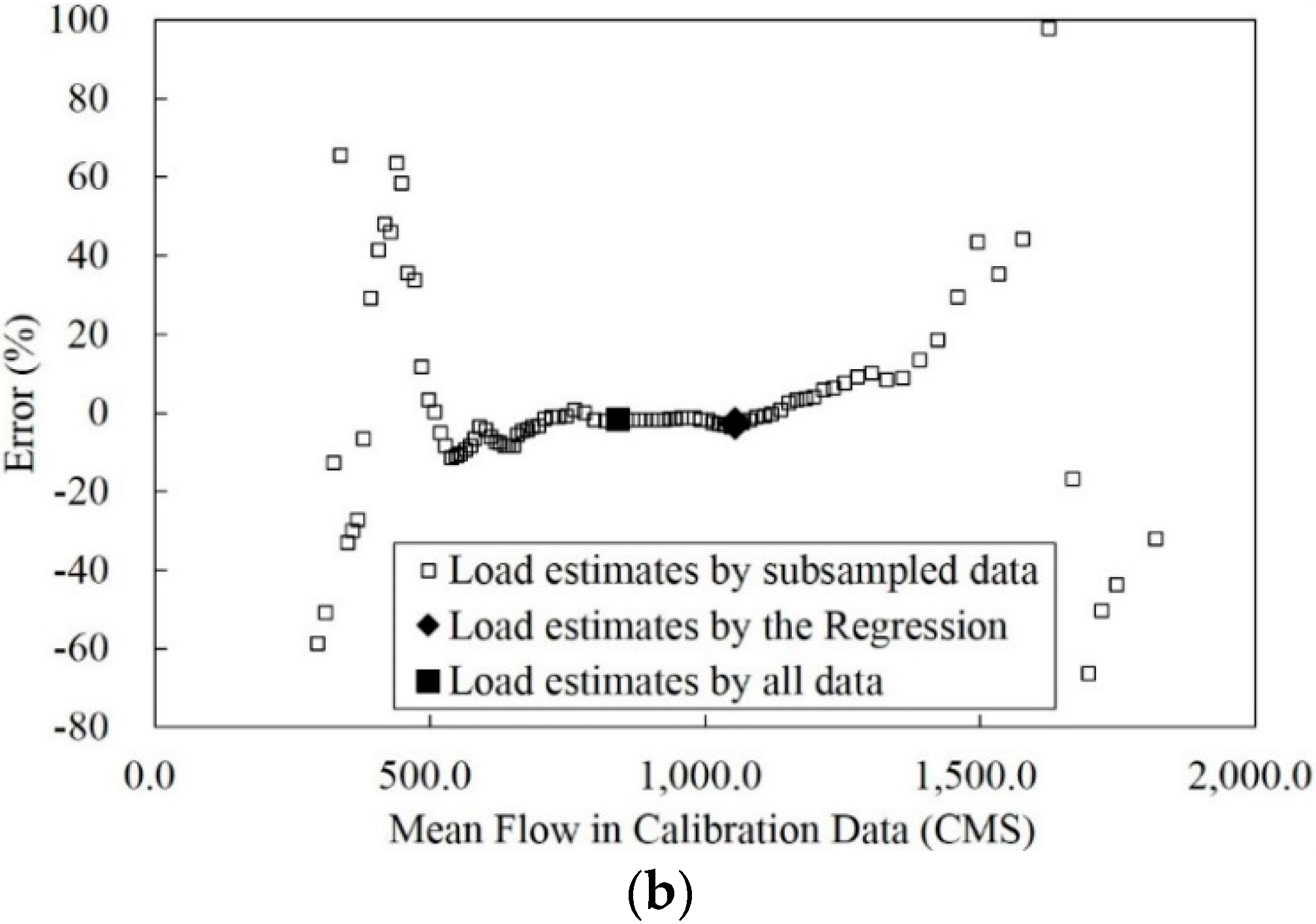
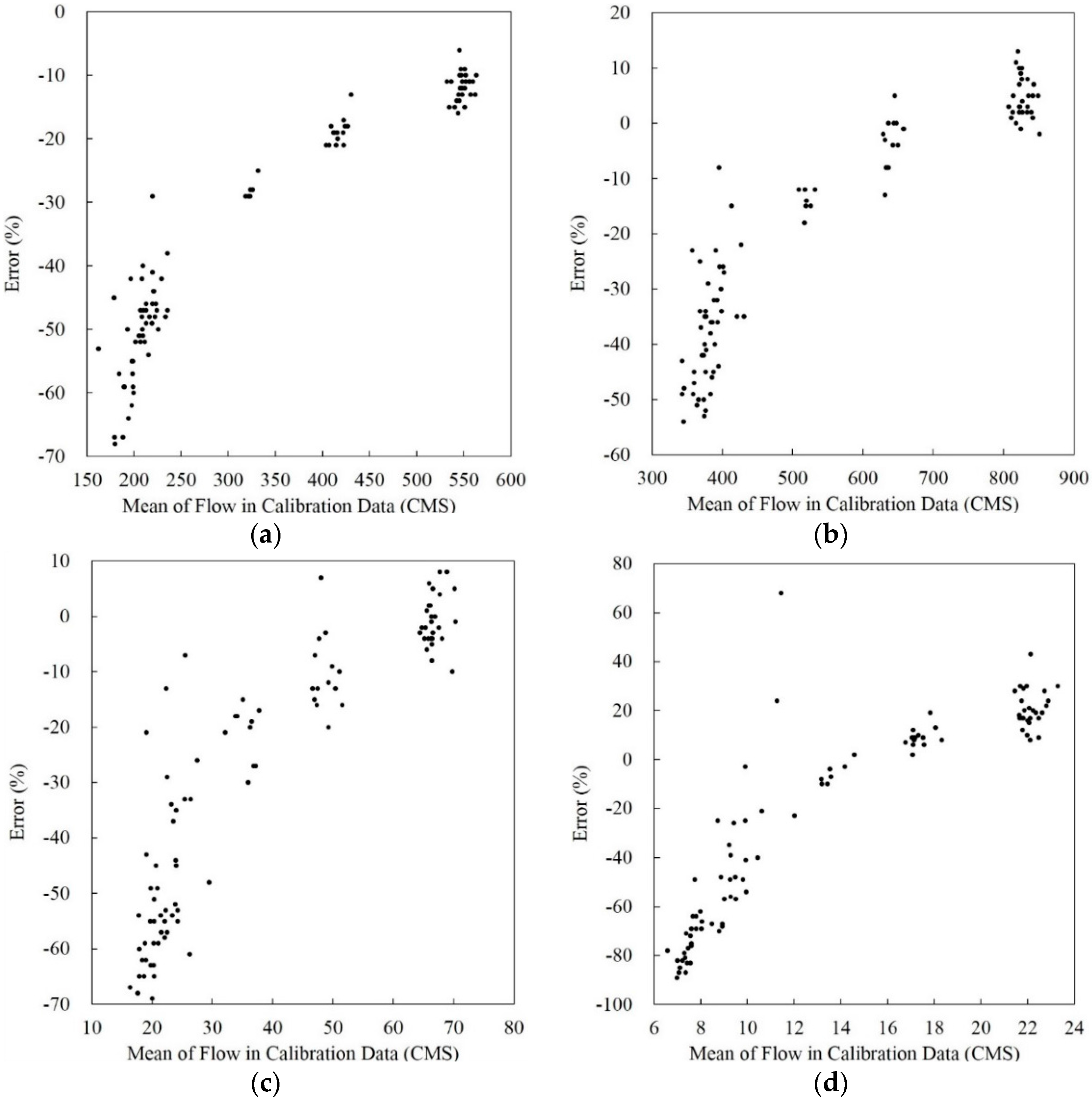
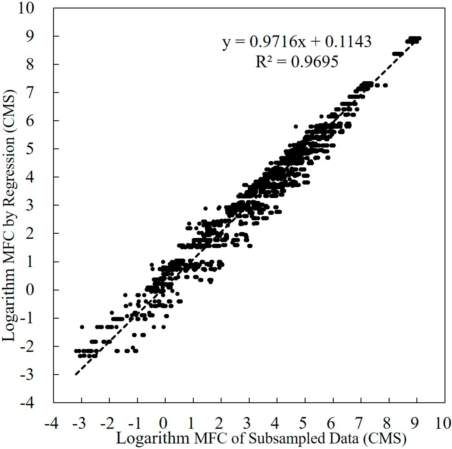
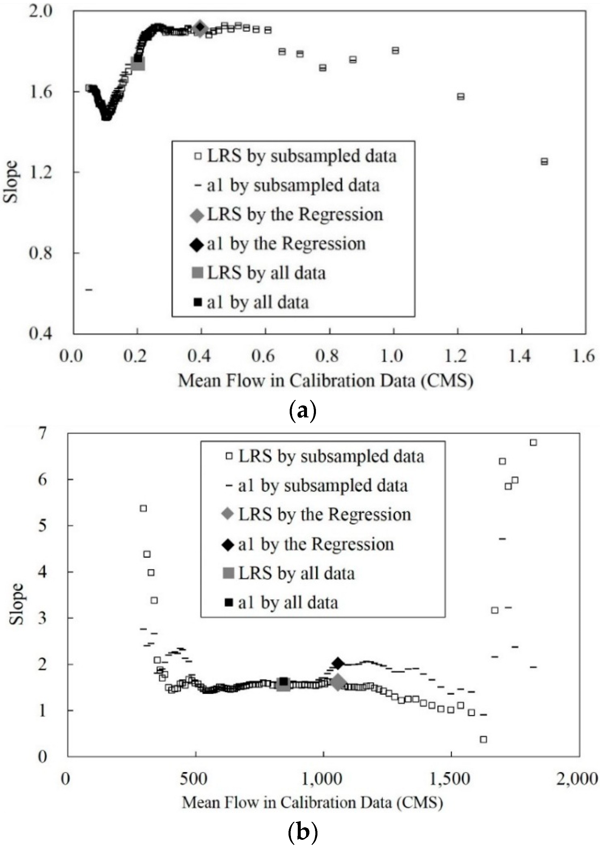
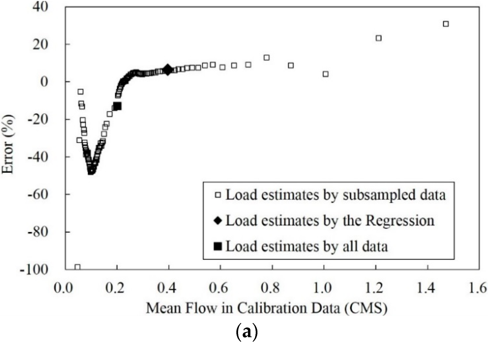
3.2. Mean Flow in Calibration Data and Annual Sediment Load Estimates

LOADEST runs were performed to identify the correlation between MFCs and annual sediment load estimates. The 10 water quality datasets from five USGS stations were subsampled based on flow size. Water quality datasets were in sequence by date, so the datasets were manipulated based on flow size in two ways to be ascending and to be descending before the data were subsampled. The first subsampled datasets from the ascending dataset were composed of the smallest 12 flow data (i.e., the smallest 12 flow data with water quality data for calibration data) from original datasets (i.e., raw-daily data), since LOADEST requires at least 12 water quality data samples with flow data. The first subsampled dataset had the minimum MFC from the original dataset. The second subsampled dataset from the ascending dataset was composed of the smallest 42 flow data from the original dataset, which was 30 flow data added to the first subsampled dataset. In the same manner, the third subsampled dataset of the ascending dataset was composed of the smallest 72 flow data form the original dataset. In other words, 30 flow data were added in each subsampling until all data were included. This approach was used to explore how LOADEST performed with data biased toward low flow. In this subsampling method, the water quality data from the largest flow were added in the last subsampling, therefore the model extrapolated with all subsampled datasets, except the last subsampled dataset which used all data.

For the method of subsampling the descending dataset, the first subsampled dataset was composed of the greatest 12 flow data from the original dataset, and the second subsampled dataset had the greatest 42 flow data. As with the other subsampling method, 30 data were added until the calibration data included all data. The first subsampled dataset had the maximum MFC from the original dataset. The annual sediment load estimates were not extrapolated, but the data were biased toward high flow (or storm events). These sampling methods are not practical in a water quality monitoring program, but they were used for evaluation of the model behaviors with MFCs.

Regression models predict loads based on the correlation between flow and water quality data. The slope, for instance a₁ in Equation (4), was regarded as one of most influential factors identifying the correlation between flow and concentration (or load). Therefore, there was a need to compare the two slopes. One was from measured data to calibrate LOADEST model coefficients, and the other was from the calibrated slope (a₁) in LOADEST. In other words, linear regression slopes (LRSs) between flow and concentration data in calibration data were computed using Equation (7), and the slope coefficients (a₁) in the LOADEST regression model (Equation (4)) were derived from all annual sediment load estimates.

Ten water quality datasets from five streams were subsampled to run LOADEST with subsampled datasets. The five USGS stations selected in the study had different geological locations and drainage areas. However, the model behaviors by changes in MFC were similar. Both LRSs (of calibration data) and a1 (from LOADEST) fluctuated when MFCs were too small or too great (Figure 4). Therefore, the errors of annual sediment load estimates were fluctuating when MFCs were too small or too great. In other words, the model showed low precision with the data biased toward either low or high flows (Figure 5). This indicates that there is a limitation on reproduction of the true load with water quality datasets biased toward low or high flow. Moreover, water quality datasets biased toward low or high flow could lead to annual sediment load estimates far from true loads. This is because the regression model requires only flow and water quality data, and therefore annual sediment load estimates close to true loads cannot be expected if the data are too biased to reproduce true load.

It might be thought that use of more water quality sample data in estimating loads would lead to pollutant load estimates that are closer to true loads. This premise was examined using all data to calibrate regression model coefficients. Although pollutant load estimates using all data were close to measured annual loads, use of all data did not necessarily lead to the smallest error in annual sediment load estimates. For instance, the error of annual sediment load estimates using all data were −13.0% and −1.7% with the data from USGS Station Number 02119400 (Figure 5a) and 06486000 (Figure 5b), while it was not difficult to find annual sediment load estimates with smaller error than the annual sediment load estimates using all data. Moreover, when MFCs were close to the required MFCs based on the regression equation (Equation (8),

Table 4. Comparison of annual sediment load estimate errors between regression equation and all data.

USGS Station Number (Data Period)	Error in Annual Sediment Load Estimates (%) (Percentage of Calibration Data from High Flow, %)
	Regression	All Data
02119400 (1959–1963)	6.4	−13.0
	(36.8)	(11.1)
02119400 (1964–1968)	2.5	−8.7
	(36.2)	(10.3)
07287150 (1993–1997)	13.0	22.4
	(16.8)	(10.1)
07287150 (1998–2002)	8.1	−5.1
	(17.4)	(10.1)
03265000 (1967–1969)	14.8	−29.5
	(20.3)	(10.1)
03265000 (1970–1973)	−10.8	−39.7
	(18.8)	(10.2)
12334550 (1993–1997)	7.5	−16.6
	(17.1)	(10.1)
12334550 (1998–2002)	0.7	−12.7
	(16.7)	(10.3)
06486000 (1992–1995)	−2.9	−1.7
	(18.4)	(10.1)
06486000 (1995–1999)	−5.8	−2.8
	(21.7)	(10.1)

), the errors were smaller than the errors of the annual sediment load estimates using all data. Therefore, a water quality dataset should consist of samples associated with appropriate flows (e.g., to be the required MFC by Equation (8)) rather than using data from extensive sampling strategies (e.g., daily water quality data collection).

The percentage of calibration data from high flow (PCH) conditions was computed in each sediment annual sediment load estimate (Table 4). High flow was defined as the upper 10% of flows for a given analysis period [35]. PCHs by the regression equation ranged from 16.7% (Station 12334550 from 1998 to 2002) to 36.8% (Station 02119400 from 1959 to 1963). Haggard et al. [18] and USGS [19] indicated 50% from water quality samples used in estimating loads should come from storm events, the percentage difference can be attributed to a different definition of storm events. For instance, Haggard et al. [18] defined storm events by flow stage exceeding 1.5 m which was approximately 20% of days during their study period, while the storm events (i.e., PCH) in the study were defined as the upper 10% of flows for a given period.

The regression equation (Equation (8)) can be employed, if the purpose of water quality monitoring programs is to estimate annual sediment loads using approaches like LOADEST:

(1)

Compute MFC_o using the regression equation with a mean flow of historical data prior to initiating a water quality monitoring program;

(2)

Collect a few water quality samples based on MFC_o;

(3)

Compute MFC_i using the regression equation with the mean flow from the beginning of water quality monitoring program;

(4)

Collect water quality samples from low flow if MFC_i is greater than the required MFC by regression equation, collect water quality samples from high flow (storm events) if MFC_i is smaller than the required MFC by regression equation;

(5)

Repeat processes 3 and 4 by the end of water quality monitoring program.

However, collecting water quality samples only for the flow regime close to the required MFC needs to be avoided, because it would be biased toward a certain regime of flow data.

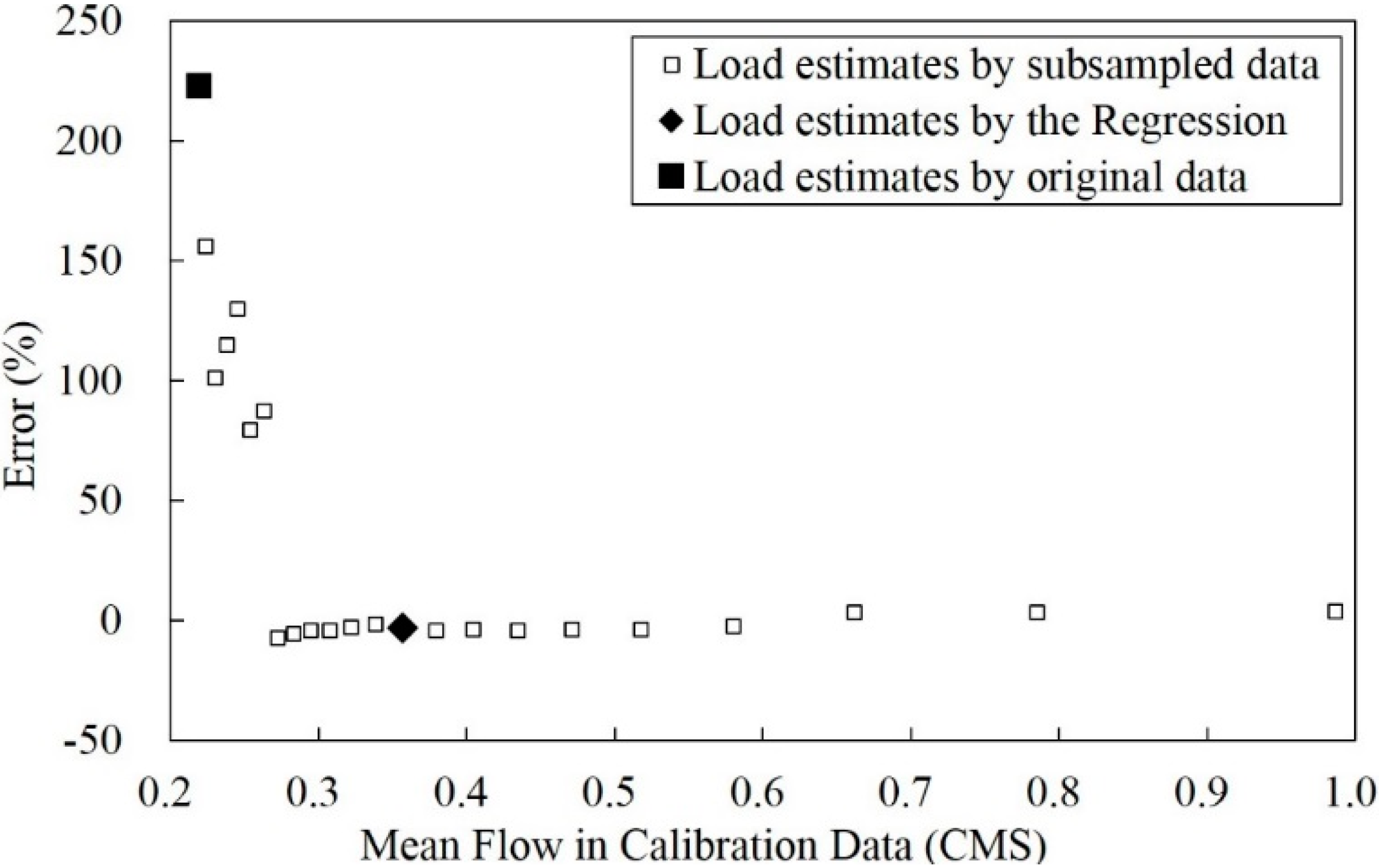
3.3. Improvement of the Poorest Annual Sediment Load Estimates

The regression equation to estimate a required MFC can be employed from the beginning of water quality monitoring programs. However, there is also a need to explore an approach to employ the regression equation for water quality datasets that have already been collected. When the regression equation is employed from the beginning of water quality monitoring programs, water quality samples will be added based on MFCs. However, if a water quality monitoring program has already been finished, or if a water quality dataset has been collected by others (e.g., EPA, USGS, etc.), water quality data cannot be added to obtain the required MFC by the regression equation. Another way to obtain the required MFC would be to exclude water quality data from the original data.

To explore this concept, five annual sediment load estimates from Park and Engel [21] were selected, which had poor annual sediment load estimates and had enough water quality data to allow data to be excluded when estimating loads. LOADEST runs were performed for the five water quality datasets, with water quality samples excluded. The water quality datasets were from monthly or fortnightly fixed interval sampling strategies, and the number of water quality data samples were 84, 120, and 261 (

Table 5. Improvement of the poorest annual sediment load estimates by MFC fitting.

USGS Station Number (Sampling Strategy)	MFE (1)	R. MFC (2)	MFC (3) (Error, %)		Num. Data (6) (PCH (7), %)
			Original (4)	Regression (5)	Original (4)	Regression (5)
02119400	0.18	0.36	0.19	0.35	120	45
(monthly on 18th)			(195.5)	(1.7)	(10.0)	(26.7)
02119400	0.18	0.36	0.22	0.36	120	57
(monthly on 19th)			(223.0)	(−3.0)	(12.5)	(26.3)
02119400	0.18	0.36	0.21	0.36	120	52
(monthly on 20th)			(132.8)	(−13.0)	(12.5)	(28.8)
02119400	0.18	0.36	0.17	0.36	261	65
(fortnightly on 12th)			(144.7)	(1.4)	(7.7)	(30.8)
05291000	1.43	2.50	1.78	2.51	84	59
(monthly on 25th)			(204.0)	(−27.0)	(9.5)	(13.6)

Notes: ⁽¹⁾ MFE: mean flow (CMS) of estimation data; ⁽²⁾ R. MFC: required MFC (CMS) by the regression equation (Equation (8)); ⁽³⁾ MFC: mean flow (CMS) of calibration data; ⁽⁴⁾ Original: calibration data from Park and Engel [21]; ⁽⁵⁾ Regression: calibration data after the exclusion of minimum flow data; ⁽⁶⁾ Num. data: the number of data in calibration data; ⁽⁷⁾ PCH: Percentage of calibration data from high flow (%).

). All MFCs from the calibration data were smaller than the required MFCs based on the regression equation. Therefore, water quality samples from the smallest flow data were removed, and LOADEST runs were performed for the reduced water quality datasets.

Annual sediment load estimates improved as water quality samples were removed. For instance, annual sediment load estimates using the original datasets showed large error, however, the error became smaller with MFC increases due to exclusion of water quality data associated with the smallest flow data (Figure 6). For the five water quality datasets, the errors ranged from 132.8% to 223.0% with the original dataset, while the errors ranged from −27.0% to 1.7% when the required MFCs from the regression equation were obtained for the LOADEST calibration datasets. The original datasets were biased toward low flow; in other words, MFCs were smaller than the required MFCs. The results indicate that a water quality dataset needs to consist of an appropriate portion of water quality data from low and high flows rather than large numbers of water quality samples, because the water quality datasets for a small number of data but with appropriate MFC demonstrated smaller errors than the water quality datasets with larger numbers of data (Table 5). The PCHs of the original datasets (‘Original’ in Table 5) were approximately 10%, while they need to be 20%–30% [21]. The PCHs of water quality datasets based on the regression equation were approximately 30%, except the water quality dataset for station 05291000 since the PCH was 13.6%.

4. Conclusions

Regression models are used to estimate pollutant loads or concentration for a given time sequence, and they are also capable of annual load estimation. LOADEST is used for various water quality parameters in various sample sizes. In the study, one of the regression models from LOADEST was evaluated with various sample sizes. Several distinct features were found in the study: (1) the mean of flow to calibrate (MFC) regression model coefficients were correlated to the mean of flow to estimate (MFE) pollutant loads; (2) the annual sediment load estimates were far from the measured loads if MFC is too small or too great; (3) the use of all data having identical data intervals and period to estimation data did not lead to the smallest error against the measured load; (4) the water quality dataset of appropriate MFC showed smaller errors than the water quality dataset for a large amount of data but biased toward low or high flows; and (5) exclusion of water quality data to fit the required MFC improved annual sediment load estimates. The results imply that a water quality dataset needs to represent the distribution of given data; in other words, it is required not to be biased toward a certain flow regime.

A regression equation was developed to compute the required mean flow in calibration data. The regression equation is applicable from the beginning of water quality monitoring programs. Furthermore, the regression equation is applicable to exclude water quality data if a water quality dataset has already been collected. The regression equation is expected to be employed, if the purpose is to estimate annual sediment loads using LOADEST.

References

1. Brigham, M.E.; Wentz, D.A.; Aiken, G.R.; Krabbenhoft, D.P. Mercury cycling in stream ecosystems. 1. Water column chemistry and transport. Environ. Sci. Technol. 2009, 43, 2720–2725. [Google Scholar] [CrossRef] [PubMed]
2. King, K.W.; Harmel, R.D. Considerations in selecting a water quality sampling strategy. Trans. ASAE 2003, 46, 63–73. [Google Scholar]
3. Halliday, S.J.; Skeffington, R.A.; Bowes, M.J.; Gozzard, E.; Newman, J.R.; Lowewnthal, M.; Palmer-Felgate, E.J.; Jarvie, H.P.; Wade, A.J. The water quality of the River Enborne, UK: Observations from high-frequency monitoring in a rural, lowland river system. Water 2014, 6, 150–180. [Google Scholar] [CrossRef] [Green Version]
4. Sanders, E.C.; Yuan, Y.; Pitchford, A. Fecal coliform and E. coli concentrations in effluent-dominated streams of the Upper Santa Cruz watershed. Water 2013, 5, 243–261. [Google Scholar] [CrossRef]
5. Valero, E. Characterization of the water quality status on a stretch of River Lerez around a small hydroeletric power station. Water 2012, 4, 815–834. [Google Scholar] [CrossRef]
6. Robertson, D.M.; Roerish, E.D. Influence of various water quality sampling strategies on load estimates for small streams. Water Resour. Res. 1999, 35, 3747–3759. [Google Scholar] [CrossRef]
7. Gilroy, E.J.; Hirsch, R.M.; Cohn, T.A. Mean square error of regression-based constituent transport estimates. Water Resour. Res. 1990, 26, 2069–2077. [Google Scholar] [CrossRef]
8. Johnson, A.H. Estimating solute transport in streams from grab samples. Water Resour. Res. 1979, 15, 1224–1228. [Google Scholar] [CrossRef]
9. Coynel, A.; Schafer, J.; Hurtrez, J.; Dumas, J.; Etcheber, H.; Blanc, G. Sampling frequency and accuracy of SPM flux estimates in two contrasted drainage basins. Sci. Total Environ. 2004, 330, 233–247. [Google Scholar] [CrossRef] [PubMed]
10. Henjum, M.B.; Hozalski, R.M.; Wennen, C.R.; Novak, P.J.; Arnold, W.A. A comparison of total maximum daily load (TMDL) calculations in urban streams using near real-time and periodic sampling data. J. Environ. Monit. 2010, 12, 234–241. [Google Scholar] [CrossRef]
11. Horowitz, A.J. An evaluation of sediment rating curves for estimating suspended sediment concentrations for subsequent flux calculations. Hydrol. Process. 2003, 17, 3387–3409. [Google Scholar] [CrossRef]
12. Johnes, P.J. Uncertainties in annual riverine phosphorus load estimation: Impact of load estimation methodology, sampling frequency, baseflow index and catchment population density. J. Hydrol. 2007, 332, 241–258. [Google Scholar] [CrossRef]
13. Kronvang, B.; Bruhnm, A.J. Choice of sampling strategy and estimation method for calculating nitrogen and phosphorus transport in small lowland streams. Hydrol. Process. 1996, 10, 1483–1501. [Google Scholar] [CrossRef]
14. Robertson, D.M. Influence of different temporal sampling strategies on estimating total phosphorus and suspended sediment concentration and transport in small streams. J. Am. Water Resour. Assoc. 2003, 39, 1281–1308. [Google Scholar] [CrossRef]
15. Cochran, W.G. Sampling Techniques, 2nd ed.; John Wiley and Sons: New York, NY, USA, 1963. [Google Scholar]
16. U.S. Environmental Protection Agency. Monitoring Guidance for Determining the Effectiveness of Nonpoint Source Controls; USEPA Office of Water Nonpoint Source Control Branch: Washington, DC, USA, 1997.
17. Zar, J.H. Biostatistical Analysis, 2nd ed.; Prentice Hall: Englewood Cliffs, NJ, USA, 1984. [Google Scholar]
18. Haggard, B.E.; Soerens, T.S.; Green, W.R.; Richards, R.P. Using regression methods to estimate stream phosphorus loads at the Illinois River, Arkansas. Appl. Eng. Agric. 2003, 19, 187–194. [Google Scholar] [CrossRef]
19. U.S. Geological Survey. Effect of Storm-Sampling Frequency on Estimation of Water-Quality Loads and Trends in two Tributaries to Chesapeake Bay in Virginia; Water-Resources Investigations Report 01-4136; U.S. Geological Survey: Richmond, VA, USA, 2001.
20. U.S. Geological Survey. Computer Programs for Describing the Recession of Ground-Water Discharge and for Estimating Mean Ground-Water Recharge and Discharge from Streamflow Records-Update; Water-Resources Investigation Report 98-4148; U.S. Geological Survey: Reston, VA, USA, 1998.
21. Park, Y.S.; Engel, B.A. Use of pollutant load regression models with various sampling frequencies for annual load estimation. Water 2014, 6, 1658–1697. [Google Scholar] [CrossRef]
22. Park, Y.S.; Engel, B.A. Analysis for regression model behavior by sampling strategy for annual pollutant load estimation. J. Environ. Qual. 2015, 44, 1843–1851. [Google Scholar] [CrossRef] [PubMed]
23. Runkel, R.L.; Crawford, C.G.; Cohn, T.A. Load Estimator (LOADEST): A Fortran Program for Estimating Constituent Loads in Streams and Rivers; U.S. Geological Survey Techniques and Methods: Reston, VA, USA, 2004.
24. Powell, J.L. Least absolute deviations estimation for the censored regression model. J. Econom. 1984, 25, 303–325. [Google Scholar] [CrossRef]
25. Jones, C.S.; Schilling, K.E. Carbon export from the Raccoon River, Iowa: Patterns, processes, and opportunities. J. Environ. Qual. 2013, 42, 155–163. [Google Scholar] [CrossRef] [PubMed]
26. Sprague, L.A.; Gronberg, J.A. Relating management practices and nutrient export in agricultural watersheds of the United States. J. Environ. Qual. 2012, 41, 1939–1950. [Google Scholar] [CrossRef] [PubMed]
27. Dornblaser, M.M.; Striegl, R.G. Suspended sediment and carbonate transport in the Yukon river basin, Alska: Flouxes and potential future responses to climate change. Water Resour. Res. 2009, 45, W06411. [Google Scholar] [CrossRef]
28. Spencer, R.G.M.; Aiken, G.R.; Bulter, K.D.; Dornblaser, M.M.; Striegl, R.G.; Hernes, P.J. Utilizing chromophoric dissolves organic matter measurements to derive export and reactivity of dissolved organic carbon exported to the Arctic Ocean: A case study of the Yukon river, Alaska. Geophy. Res. Lett. 2009, 36, L06401. [Google Scholar] [CrossRef]
29. Carey, R.O.; Migliaccio, K.W.; Brown, M.T. Nutrient discharges to Biscayne Bay, Florida: Trends, loads, and a pollutant index. Sci. Total Environ. 2011, 409, 530–539. [Google Scholar] [CrossRef] [PubMed]
30. Das, S.K.; Ng, A.W.M.; Perera, B.J.C. Assessment of nutrient and sediment loads in the Yarra river catchment. In Proceedings of the 19th International Congress on Modelling and Simulation, Perth, Australia, 12–16 December 2011; pp. 3490–3496.
31. Oh, J.; Sankarasubramanian, A. Interannual hydroclimatic variability and its influence on winter nutrients variability over the southeast United States. Hydrol. Earth Syst. Sci. Discuss. 2011, 8, 10935–10971. [Google Scholar] [CrossRef]
32. Duan, S.; Kaushal, S.S.; Groffman, P.M.; Band, L.E.; Belt, K.T. Phosphorus export across an urban to rural gradient in the Chesapeake Bay watershed. J. Geophy. Res. 2012, 117. [Google Scholar] [CrossRef]
33. USGS Water Quality Data for the Nation Homepage. Available online: http://waterdata.usgs.gov/nwis/qw (accessed on 23 March 2013).
34. National Center for Water Quality Research of Heidelberg University Homepage. Available online: http://www.heidelberg.edu/academiclife/distinctive/ncwqr (accessed on 23 March 2013).
35. U.S. Environmental Protection Agency. An Approach for Using Load Duration Curves in the Development of TMDLs; US EPA Office of Wetlands, Ocean and Watersheds: Washington, DC, USA, 2007.
36. R Core Team. R: A Language and Environment for Statistical Computing. R Foundation for Statistical Computing; The R Foundation: Vienna, Austria, 2012. [Google Scholar]
Figure 1. Correlation between errors and mean of flow in calibration data: (a) USGS station number 01357500; (b) USGS station number 01463500; (c) USGS station number 01470500; (d) USGS station number 01481000.
Water 08 00368 g001
Figure 2. Correlation between mean of flows in calibration and estimation data.
Water 08 00368 g002
Figure 3. Comparison of means of flow to calibrate (MFCs) from the calibration data of acceptable annual sediment loads and the required MFCs by Equation (8).
Water 08 00368 g003
Figure 4. Comparison of slopes from linear regression formula (LRS in Equation (7)) and calibrated LOADEST model (a1 in Equation (4)): (a) USGS station number 02119400; (b) USGS station number 06486000.
Water 08 00368 g004
Figure 5. Annual sediment load estimates by MFCs: (a) USGS station number 02119400; (b) USGS station number 06486000.
Water 08 00368 g005aWater 08 00368 g005b
Figure 6. Annual sediment load estimate improvement when excluding water quality samples (USGS station number 02119400, monthly fixed sampling strategy on 19th of every month).
Water 08 00368 g006