Estimated Grass Grazing Removal Rate in a Semiarid Eurasian Steppe Watershed as Influenced by Climate

Abstract

Grazing removal rate of grasses needs to be determined for various climate conditions to address eco-environmental concerns (e.g., desertification) related to steppe grassland degradation. The conventional approach, which requires survey data on animal species and heads as well as grass consumption per individual animal, is too costly and time-consuming to be applied at a watershed scale. The objective of this study was to present a new approach that can be used to estimate grazing removal rate with no requirement of animal-related data. The application of this new approach was demonstrated in a Eurasian semiarid typical-steppe watershed for an analysis period of 2000 to 2010. The results indicate that the removal rate tended to become larger, but its temporal variation tended to become smaller, from the upstream to downstream. Averaged across the watershed, the removal rate ranged from 63.9 to 401.0 g DM m⁻² (or 22.4 to 60.9%) during the analysis period. As expected, the removal rate in an atmospherically wetter year was higher than that in an atmospherically drier year. Nevertheless, none of the eleven analysis years had a removal rate higher than the threshold value of 65%, above which the risk of grassland degradation would become much greater.

1. Introduction

Steppe grasslands occupy about 8% of the earth’s terrestrial surface and are now considered the most altered and beleaguered ecosystem on the planet [1]. Over 40% of the global grasslands have been somewhat altered from their indigenous state, including more than 70% of the Inner Mongolia steppe grasslands of China [2], which are part of the largest and most characteristic Eurasian grassland (or Great Steppe). Here, the degradation has caused serious environmental and ecological problems such as more frequent and damaging hydrologic extremes (i.e., floods and droughts), desertification, dust storms, and even commodity scarcity. These problems in turn will likely threaten the sustainability of “grassland agriculture,” a system of agriculture in which major emphasis is placed on grasses, legumes, and other fodder or soil-building crops [3]. The main factors causing degradation are overgrazing, cultivation, overdevelopment, and climate change [4,5,6,7,8], which have altered the natural hydrology [9] and led to the erosion of the 10 to 20 cm calcic castanozem topsoil. This topsoil is vital for efforts to sustain grasslands because it is loose and has a plentiful supply of humus/organic matter. Policy choices to reduce or reverse grassland degradation are often made with only a vague understanding of causative complexity among steppe hydrology, topsoil erosion, and grassland degradation, however, which can limit efforts to manage, protect and/or restore steppe grasslands.

In order to fill this knowledge gap, the grazing removal rate of grasses needs to be determined for various climate conditions as characterized by precipitation and evapotranspiration. The conventional approach consists of that: (1) an extensive survey is conducted household by household to obtain data on species and heads of all grass-grazing animals (i.e., cows, horses, and sheep); (2) for a given animal species, the grazing rate was computed as the multiplication of the heads of this species and the dry mass (DM) of grass eaten by one such animal per year; and (3) the total grass removal rate in an area of interest is computed as the summation of the grazing rates of all animal species. Such a conventional approach can become too costly and time-consuming to be implemented for multiple years at a watershed scale as required to effectively manage steppe grasslands in practice. This may be an important reason why few watershed-scale studies on grazing removal rate have been reported in existing literature. The objective of this study was to present an innovative method that can be used to accurately estimate grazing removal rate at a watershed scale using remote sensing images and a total net primary production (NPP) prediction model. Hereinafter, NPP is the summation of aboveground (i.e., stems and leaves) and belowground (i.e., roots) productions. One advantage of this method over the conventional approach is that this method does not require data on animals. The rationale of this method is that NPP can well reflect the physical link between biosphere and climate system through the global cycling of carbon, water and nutrients, and can be reduced by grazing as a primary mechanic mechanism. This study applied and tested this method in a Eurasian semiarid typical-steppe watershed to be described in Section 2.1.

2. Materials and Methods

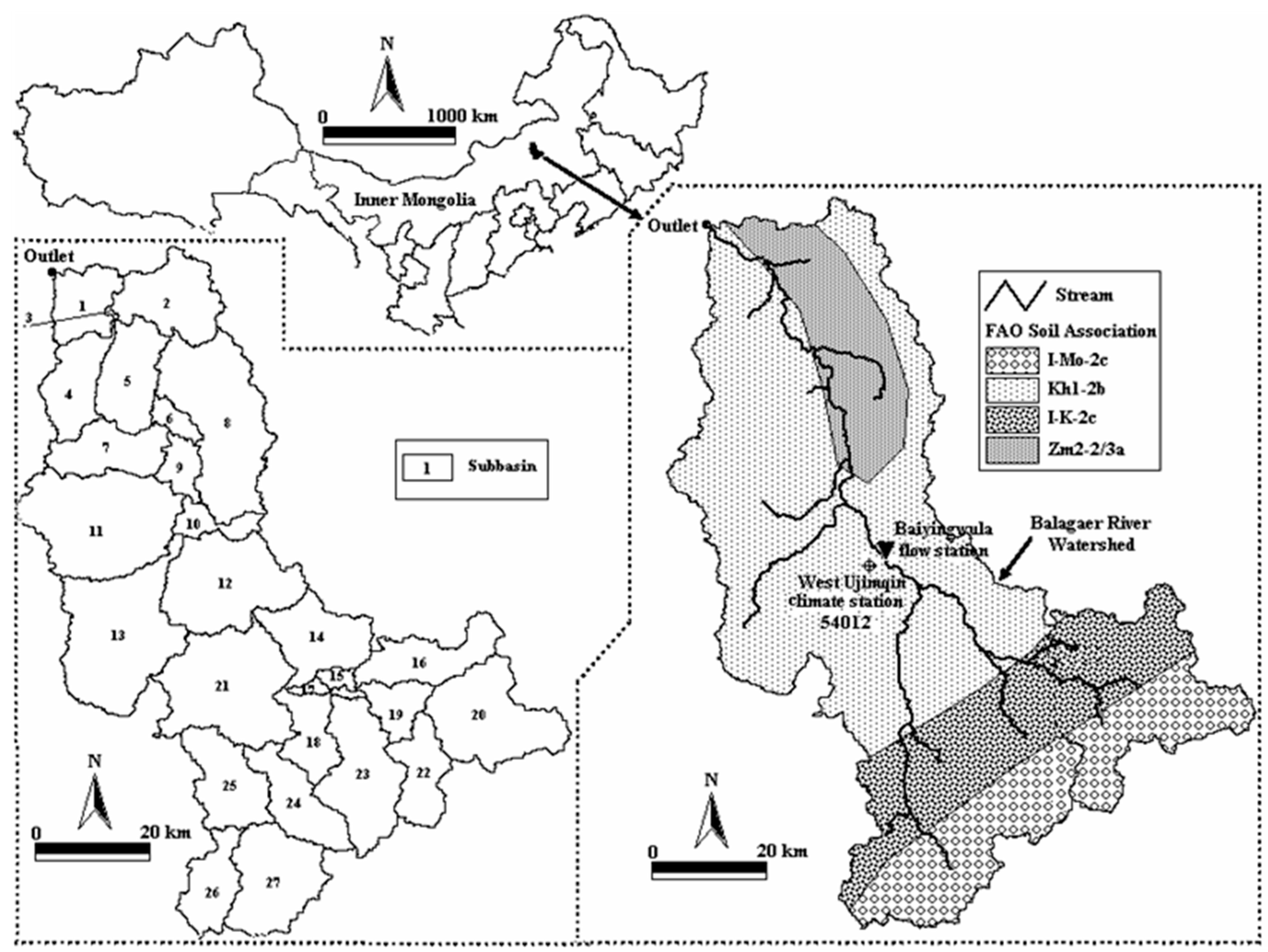
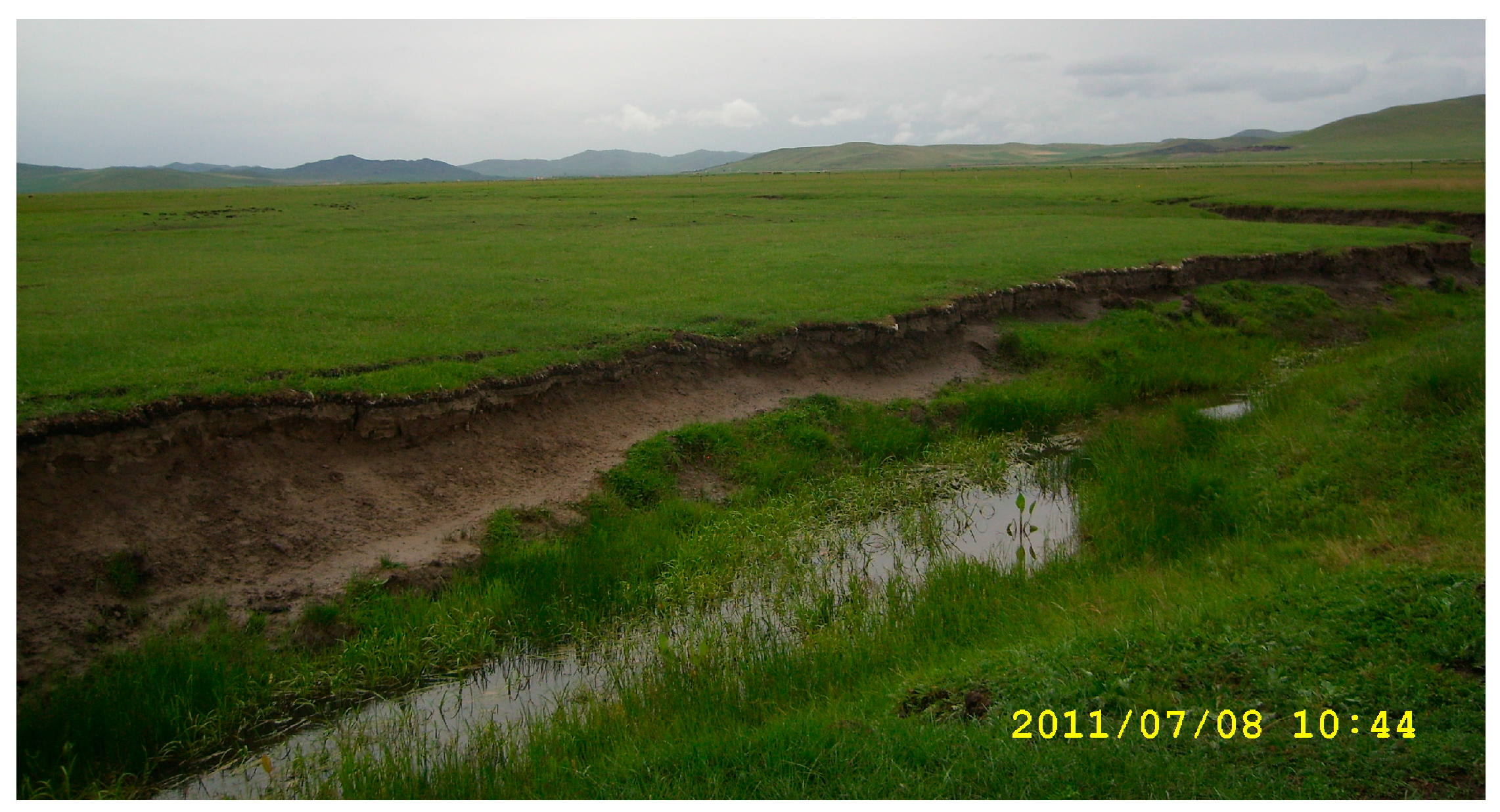
2.1. The Study Watershed

The 5350 km² Balagaer River watershed (centroid: 117°36′ E, 44°35′ N), located in the northeast Inner Mongolia Autonomous Region of China (Figure 1), was selected for this study. This watershed is almost uniformly covered by typical steppe grasses (Figure 2), with the predominant species of Leymus chinensis and Stipa grandis. The grasses, which are solely fed by rainwater and dependent on naturally-available nutrients (e.g., animal manures), have a root depth of up to 60 cm [10]. Rarely harvested, most of the grasses are mainly removed by semi-nomadic-style (i.e., half-year) grazing. The elevation of the watershed varies from 980 to 1876 m above mean sea level, with a mean topographic gradient of 0.09. The soils are classified by the Food and Agriculture Organization of the United Nations [11] into four classes, namely I-Mo-2c, Kh1-2b, I-K-2c, and Zm2-2/3a (Figure 1), each of which is further subdivided into two (i.e., upper and lower) layers. The first three types of soils are more permeable than the fourth. The upper layer is from ground surface to the 30 cm depth, while the lower layer is from the 30 to 100 cm depth. Across the watershed, the saturated hydraulic conductivity (K_s) varies from 1.5 to 107.0 mm·h⁻¹, with a mean of 28.5 mm·h⁻¹. The loamy soils are composed of less than 30% clay particles (diameter less than 0.002 mm) and more than 70% sand (diameter from 0.05 to 2.0 mm) and silt (diameter from 0.002 to 0.05 mm) particles [12].

The watershed receives 170 to 615 mm precipitation annually, with a mean of 335 mm. Most of the precipitation falls between July and September as rain, and between October and January as snow. However, the watershed has an annual potential evapotranspiration (E₀) of 1165 mm or higher, which is much larger than the mean annual precipitation, so the watershed has an arid and semiarid climate (i.e., is water-limited). The annual mean daily average air temperature is 1.2 °C, with a maximum daily temperature of up to 37.5 °C in summer and a minimum daily temperature of as low as −38.5 °C in winter. The watershed has an annual mean daily average wind speed of about 15 km·h⁻¹, with between 28 and 148 windy days in any given year. On a windy day, the maximum wind speed can reach 125 km·h⁻¹. The watershed has an annual mean discharge of 0.33 m³·s⁻¹, and the major water users are agriculture, animal husbandry, domestic, and power industry [13].

2.2. Data and Preprocessing

Daily data on precipitation, air temperature, relative humidity, wind speed, and solar radiation at West Ujimqin Climate Station 54012 (Figure 1) were downloaded from the National Meteorological Information Center website [14] for a record period of 1 January 2000 to 31 December 2010. This study presumed that precipitation was spatially uniform across the watershed for three reasons. First, there was no any other climate station within or adjacent to the watershed, where long-term observations were available. Second, given that West Ujimqin Climate Station is located near the centroid of the watershed, the station could likely represent the primary climate conditions for the entire drainage area. Thirdly, using the data on precipitation measured from 2010 to 2012 at 15 raingauges, which were installed and maintained by the authors across the watershed, Luo et al. [15] found that the precipitation exhibited a minimal spatial variation. In fact, the sufficient spatial coverage of climate stations and/or raingauges has been, and will continue to be, a challenge for any hydrology-related studies provided that the insufficient coverage tends to under-represent the possible spatial heterogeneity of precipitation. Global efforts are underway to use modern technologies (e.g., next generation radar) to acquire precipitation data at a kilometer spatial resolution [16]. However, such high-resolution data are just available for a few experiment sites and can have large uncertainties [17].

In addition, a soil classification GIS (geographic information system) map and its associated attribute table were downloaded from the FAO website [18]. The GIS map subdivides the watershed into 22 map units (not shown), each of which is assigned one of the four classes mentioned in Section 2.1, as shown in Figure 1. For each soil map unit and layer, the attribute table defines its soil texture (i.e., percent sand, silt, and clay particles) and organic matter content. In this study, the information presented by the attribute table was used to estimate the intrinsic soil-water properties (e.g., permanent wilting point ψ, field capacity ${\mathsf{\theta }}_{\mathrm{fc}}$, and saturated soil moisture ${\mathsf{\theta }}_{\mathrm{sat}}$) [19]. ψ is the minimal point of soil moisture the plant requires not to wilt, ${\mathsf{\theta }}_{\mathrm{sat}}$, on the other hand, is the soil moisture when all pores in the soil are filled with water. ${\mathsf{\theta }}_{\mathrm{fc}}$ is the soil moisture after the soil is saturated and then allowed to drain by water gravity until the drainage ceases. Further, a 30-m digital elevation model (DEM), which is a 3D representation of the watershed’s terrain surface with a spatial resolution of 30 m, was downloaded from the International Scientific Data Service Platform website http://datamirror.csdb.cn and used to delineate the boundary of the study watershed and its subbasins. As a result of the delineation, the watershed was subdivided into 27 subbasins (Figure 1).

Further, data on annual NPP, in g C m⁻², were extracted using the ENVI^® 4.7 software package from the 1-km MODIS (Moderate Resolution Imaging Spectroradiation) 17A3 images for the period of 2000 to 2010. The images, downloaded from the U.S. Geological Survey (USGS) Land Processes Distributed Active Center (LPDAC) website [20], present values of annual NPP [21,22,23,24]. Firstly, in ArcGIS^® 10, the images that cover the study watershed were merged into a single image, which was then projected to the coordinate system of the Universal Transverse Mercator (UTM) zone 50 N. Secondly, the projected image was clipped to the spatial extent of the watershed and then overlaid with the subbasin map delineated above. Thirdly, for each year, the NPP values for the 1-km cells that are included within a subbasin were arithmetically averaged to get the NPP value of this subbasin, and then the NPP values for the 27 subbasins were area-weighted averaged to get the NPP value of the study watershed as a whole. As a result, 28 NPP time series (one for the watershed and 27 for the subbasins) were generated. Finally, for a given subbasin, the NPP values for the analysis years (2000 to 2011) were arithmetically averaged to get the annual mean NPP of this subbasin.

2.3. Description of the NPP-Prediction Model

This study modified and used an NPP-prediction model developed by [13]. This empirical model estimates NPP, in g DM m⁻², as:

$$\mathrm{NPP}=100\cdot \mathrm{RDI}\cdot \mathrm{E}\cdot \exp \left[-{\left(9.87+6.25\cdot \mathrm{RDI}\right)}^{0.5}\right]$$

(1)

where RDI (-) is the dimensionless climatic dryness index; E (mm) is the annual actual evapotranspiration; and 100 is a unit conversion factor.

RDI is computed as [25]:

$$\mathrm{RDI}=0.629+0.237\cdot \left(\frac{{\mathrm{E}}_0}{\mathrm{P}}\right)-0.00313\cdot {\left(\frac{{\mathrm{E}}_0}{\mathrm{P}}\right)}^2$$

(2)

where E₀ (mm) is the annual potential evapotranspiration; and P (mm) is the annual precipitation.

E is estimated using a modified theoretical Fu’s solution [26,27,28] to the hypothesis of [29]. The Budyko hypothesis describes the annual water balance as a function of available water and energy, and it has been tested all over the world and widely used to estimate E [30,31,32]. However, because the original Fu’s solution (used in [13]) assumes that E ≤ P, which can be invalid when P is small in a water-limited environment [33], which is the case of the Balagaer River watershed, this study developed a modified solution by introducing a soil-moisture enhancement factor to take into account the evapotranspiration portion beyond P. Albeit, both the modified and original Fu’s solution share a same assumption of negligible water storage change within the analysis time interval. This assumption is usually valid for arid and semiarid areas at a large (e.g., annual) time interval [34]. The modified Fu’s solution is expressed as:

$$\frac{\mathrm{E}}{{\mathsf{\alpha }}_{\mathrm{sm}}\cdot \mathrm{P}}=1+\frac{{\mathrm{E}}_0}{{\mathsf{\alpha }}_{\mathrm{sm}}\cdot \mathrm{P}}-{\left[1+{\left(\frac{{\mathrm{E}}_0}{{\mathsf{\alpha }}_{\mathrm{sm}}\cdot \mathrm{P}}\right)}^{\mathsf{\omega }}\right]}^{\frac{1}{\mathsf{\omega }}}$$

(3)

where α_sm (≥1) (-) is the soil-moisture enhancement factor, representing the compensation of soil moisture to the portion of E beyond P; ω (-) has a range of [1, +∞) and is a parameter that represents combined effects of subbasin characteristics (namely vegetation physiology, soil properties, and topography) on water balance.

Yang et al. [30] presented a formula for ω. This formula (used in [13] considers soil properties and topography, but it does not have any variable representing vegetation physiology. Based on basic principles of hydrology [35] and findings of [36], a vegetation canopy can enhance evapotranspiration, that is, E tends to become larger for an area with a vegetation canopy than for the same area without the canopy. The enhancement depends on vegetation physiologic characteristics, namely species, stem height, leaf structure, and root structure. With this regard, this study introduced a vegetation-specific enhancement factor as a multiplier into the formula of [30], resulting in a new formula for ω expressed as:

$$\mathsf{\omega }=\left\{1+8.652\cdot {\left(\frac{{\mathrm{K}}_{\mathrm{s}}}{\mathrm{P}/{\mathrm{D}}_{\mathrm{w}}}\right)}^{-0.368}\cdot {\left(\frac{{\mathrm{S}}_{\max }}{{\mathrm{E}}_0}\right)}^{0.463}\cdot \exp \left[-4.464\cdot \tan \left(\mathsf{\beta }\right)\right]\right\}\cdot {\mathsf{\alpha }}_{\mathrm{veg}}$$

(4)

where D_w (-) is the number of wet days with nonzero precipitation; K_s (mm·day⁻¹) is the saturated hydraulic conductivity; S_max = (θ_fc − ψ)·d_r (mm) is the available water capacity of root zone; d_r (mm) is the root depth; β (°) is the landscape slope angle; and α_veg (≥1) (-) is the vegetation-specific enhancement factor.

Because the Penman-Monteith formula [37] is physically based and the best predictor of potential evapotranspiration (PET) among the existing evaporation models [38,39], it was chosen to estimate daily PET (mm·day⁻¹), which was summed spanning a year to get E₀ in this NPP-prediction model. The formula can be expressed as:

$$\mathrm{PET}=\frac{0.408\cdot \mathsf{\Delta }\cdot \left({\mathrm{R}}_{\mathrm{n}}-\mathrm{G}\right)+\mathsf{\gamma }\cdot \frac{900}{{\mathrm{T}}_{\mathrm{air}}+273}\cdot {\mathrm{u}}_2\cdot \left({\mathrm{e}}_{\mathrm{s}}-{\mathrm{e}}_{\mathrm{a}}\right)}{\mathsf{\Delta }+\mathsf{\gamma }\cdot \left(1+0.34\cdot {\mathrm{u}}_2\right)}$$

(5)

where Δ (kPa·°C⁻¹) is the slope of saturation vapor pressure curve; R_n (MJ m⁻²·day⁻¹) is the net solar radiation at vegetation surface; G (MJ m⁻²·day⁻¹) is the soil heat flux density; γ (kPa·°C⁻¹) is the psychrometric constant; T_air (°C) is the mean air temperature at 2 m height above ground surface; u₂ (m·s⁻¹) is the wind speed at 2 m height above ground surface; e_s (kPa) is the saturation vapor pressure; and e_a (kPa) is the actual vapor pressure. These parameters can be determined using the procedure recommended by [11].

T_air is computed as:

$${\mathrm{T}}_{\mathrm{air}}=\frac{{\mathrm{T}}_{\min }+{\mathrm{T}}_{\max }}{2}$$

(6)

where T_min (°C) and T_max (°C), respectively, are the daily minimum and maximum air temperatures.

Δ is computed as:

$$\mathsf{\Delta }=\frac{{\left(0.00815\cdot {\mathrm{T}}_{\mathrm{air}}+0.8912\right)}^7}{10}$$

(7)

γ is computed as:

$$\mathsf{\gamma }=6.6\times {10}^{-4}\cdot {\mathrm{P}}_{\mathrm{atm}}$$

(8)

where P_atm (kPa) is the atmosphere pressure, and it equals to 101.3 kPa at the mean sea level and a temperature of 20 °C [40].

e_s is computed as:

$${\mathrm{e}}_{\mathrm{s}}=\frac{1}{2}\cdot \left[\exp \left(\frac{16.78\cdot {\mathrm{T}}_{\min }-116.9}{{\mathrm{T}}_{\min }+237.3}\right)+\exp \left(\frac{16.78\cdot {\mathrm{T}}_{\max }-116.9}{{\mathrm{T}}_{\max }+237.3}\right)\right]$$

(9)

e_a is computed as:

$${\mathrm{e}}_{\mathrm{a}}=\mathrm{RH}\cdot {\mathrm{e}}_{\mathrm{s}}$$

(10)

where RH (percentage) is the relative humidity.

When dew point temperature, T_d (°C), is given and if 0 °C < T_air < 60 °C, 0 °C < T_d < 50 °C, and 1% < RH < 100%, RH can be computed as:

$$\mathrm{RH}=\frac{\exp \left(\frac{17.271\cdot {\mathrm{T}}_{\mathrm{d}}}{237.7+{\mathrm{T}}_{\mathrm{d}}}\right)}{\exp \left(\frac{17.271\cdot {\mathrm{T}}_{\mathrm{air}}}{237.7+{\mathrm{T}}_{\mathrm{air}}}\right)}$$

(11)

When wind speed is measured at a height different from 2 m above the ground, it can be converted to u₂ using a logarithmic profile formula found in [41,42]. R_n can be directly measured or estimated based on the extraterrestrial solar radiation and air temperatures [35,43].

2.4. Parameterization of the NPP-Prediction Model

For each soil map unit, the soil-water parameters, including$\mathsf{\psi }$, ${\mathsf{\theta }}_{\mathrm{fc}}$, ${\mathsf{\theta }}_{\mathrm{sat}}$, and ${\mathrm{K}}_{\mathrm{s}}$, were estimated using the soil-plant-air-water (SPAW) model [18]. The model uses a set of empirical equations to formulate the soil-retention curves in terms of the soil texture. The curves include the pressure-moisture curve, which describes the continuous relationship between capillary pressure and soil-water moisture content, and the conductivity-moisture curve, which describes the relationship between hydraulic conductivity and soil-water moisture content. In general, a pressure-moisture curve consists of three segments [44,45]: the first segment is continuous and nonlinear for capillary pressures between 1500 and 10 kPa, the second segment is linear for capillary pressures between 10 kPa to the air-entry capillary pressure, and the third segment has constant water content for capillary pressures smaller than the air-entry capillary pressure. In contrast, the conductivity-moisture curve is continuous and nonlinear from the saturation moisture content (${\mathsf{\theta }}_{\mathrm{sat}}$) to near air dry. Those empirical equations, described in detail in [46], have been proved to be valid for a wide range of textures. The inputs of the SPAW model include percentages of sand and clay particles, and the average organic matter content within a soil map unit of interest. In addition, the ArcGIS^® Hydrology extension was used to process the DEM to delineate the boundary of the Balagaer River watershed and its subbasins. As a result of the delineation, the watershed was subdivided into 27 subbasins (Figure 1), each of which was assumed to have a uniform overland gradient (i.e., single value for β). The extension automatically calculated β for the subbasins from the elevation values presented by the DEM.

Further, the subbasin map and the soil map were overlain in ArcGIS^® to determine the areal proportion of a given soil map unit that is included in each of the subbasins. Afterward, for each of the four parameters (i.e., $\mathsf{\psi }$, ${\mathsf{\theta }}_{\mathrm{fc}}$, ${\mathsf{\theta }}_{\mathrm{sat}}$, and ${\mathrm{K}}_{\mathrm{s}}$), the area-weighted average of its values responding to the map units that are included in a subbasin was computed and taken as the value of this parameter for this subbasin. Moreover, this study assumed that d_r (=60 cm), P_atm (=101.3 kPa), α_sm, and α_veg are spatiotemporally invariant. α_sm and α_veg were empirically adjusted until $\frac{\mathrm{E}}{\mathrm{P}}$ for the watershed and its subbasins falls between 0.85 to 1.35 for all eleven analysis years. This range of $\frac{\mathrm{E}}{\mathrm{P}}$ was determined by [33] based on field measurements and the FAO-56 (Food and Agriculture Organization Irrigation and Drainage Paper No. 56) dual crop coefficient (DCC) method [47,48] in the Xilin River Basin (115°32′ to 117°36′ E, 43°26′ to 44°39′ N), which is adjacent to the Balagaer River watershed.

2.5. Analysis of Grazing Removal Rate

For a given year, the value predicted by the model (Equation (1)) is the NPP with no influence of grazing and was thus presumed as the “natural” NPP, whereas the value presented by the MODIS data reflects the ground truth and was considered as the “actual” NPP. With a typical carbon content of 70% in dry leaves/stems plus roots of steppe grasses (including Leymus chinensis and Stipa grandis) [49], the MODIS-presented actual NPP (in g C m⁻²) was divided by this carbon content to have consistent units with the mode-predicted natural NPP (in g DM m⁻²). For the simplicity, by assuming that grazing and climate independently (but not interactively) influenced grass production, this study computed grass removal rate as difference of natural NPP less actual NPP. Although previous field experiments (e.g., [50,51,52]) found that the grass production in a dry year was mainly controlled by precipitation and temperature while the grass production in a wet year was primarily affected by grazing, [53] postulated that grazing and climate can somewhat interactively influence grass production and that such an interactive influence can either be positive or negative, depending on a number of not-easy-to-be-quantified factors (e.g., grazing intensity and pattern). Thus, our simple method may overestimate the grass removal rate for one year, while it can underestimate the grass removal rate for another year. However, for a long-term average, the overestimations and underestimations can be expected to be canceled out, making the method be a good predictor of annual mean NPP.

The computation, which was done on a yearly basis for each of the 27 subbasins as well as for the study watershed as a whole, resulted in 28 time series of removal rate in g DM m⁻², which in turn were divided by the corresponding 28 time series of natural NPP in g DM m⁻² to derive another 28 time series of removal rate in percent. Totally, 112 (4 × 28) time series, each of which has a length of N = 11 years, were obtained: 28 for natural NPP, 28 for actual NPP, 28 for removal rate in g DM m⁻², and 28 for removal rate in percent. Please note that four of the 112 time series were for the watershed and the remaining 108 time series were for the subbasins. In addition, 58 time series (with a same length of N = 11 years) of climate factors were also derived: one for P, 28 for E, 28 for $\frac{\mathrm{E}}{\mathrm{P}}$, and one for$\frac{{\mathrm{E}}_0}{\mathrm{P}}$. Further, across the 27 subbasins, the maximums and minimums of natural NPP, actual NPP, removal rate in g DM m⁻², and removal rate in percent, were computed, resulting in eight more time series of extreme values, each of which has a length of N = 11 years.

Firstly, the eight time series of extreme values and the four time series for the watershed were plotted to visually examine the spatiotemporal variations of NPP and removal rate. Secondly, at the watershed scale, the removal rate in percent was plotted versus each of the four climate factors (i.e., P, E, $\frac{\mathrm{E}}{\mathrm{P}}$, and $\frac{{\mathrm{E}}_0}{\mathrm{P}}$) to visually examine overall influences of climate on grazing removal rate. Finally, at both the watershed and subbasin scales, Pearson correlation coefficients [54] were computed between removal rate (either in g DM m⁻² or percent) and each of the four climate factors, and then compared with a critical value r_c (Equation (12)) for a significance level of α = 0.05 to identify which climatic condition (e.g., drier versus wetter) might be more closely associated with a higher grazing removal rate. A climate factor that gives a Pearson correlation coefficient (in absolute) of greater than r_c was judged to have a significant (at α = 0.05) influence on grass removal.

$${\mathrm{r}}_{\mathrm{c}}=\frac{{\mathrm{t}}_{\mathsf{\alpha }}}{\sqrt{{\mathrm{t}}_{\mathsf{\alpha }}^2+\mathrm{N}-2}}$$

(12)

where N (years) is the length of time series; and t_α (-) is the critical value of a t-distribution with N − 2 freedom and at a two-tail exceedance probability of α. Here, ${\mathrm{r}}_{\mathrm{c}}=\frac{2.262}{\sqrt{{\left(2.262\right)}^2+11-2}}=0.60$.

3. Results

3.1. The Parameterized Model

The sizes of the delineated subbasins ranged from 3 to 458 km², with a mean of 198 km². As expected, the subbasins that are directly drained by the lower reach of the Balagaer River (e.g., subbasins 3 and 6) were determined to have a smaller landscape slope angle than the subbasins near the watershed upper boundary (e.g., subbasins 20 and 26) (Figure 1 and

Table 1. The adopted values of the model parameters in this study ^†.

Subbasin ‡	Area (km2)	β (°)	ψ	θfc	θsat	Ks (mm·h−1)	ω
1	140	3.36	0.155	0.323	0.481	11.33	3.901
2	222	2.87	0.155	0.323	0.481	11.33	3.955
3	3	1.29	0.137	0.317	0.480	12.59	4.144
4	163	3.45	0.237	0.392	0.514	4.64	4.381
5	195	2.65	0.164	0.320	0.473	9.75	4.022
6	40	1.54	0.156	0.311	0.471	11.31	4.072
7	172	2.70	0.103	0.232	0.458	34.18	3.385
8	453	2.58	0.103	0.232	0.458	34.18	3.394
9	67	1.89	0.050	0.104	0.462	107.48	2.908
10	66	2.68	0.051	0.120	0.460	96.74	2.961
11	458	2.30	0.131	0.286	0.465	15.75	3.812
12	351	4.04	0.050	0.107	0.461	105.30	2.876
13	455	3.39	0.126	0.270	0.460	18.24	3.608
14	211	3.39	0.140	0.295	0.467	13.86	3.762
15	23	2.64	0.140	0.295	0.467	13.86	3.839
16	169	6.46	0.237	0.382	0.504	4.64	3.941
17	23	2.89	0.113	0.283	0.469	18.80	3.722
18	127	3.27	0.113	0.283	0.469	18.80	3.686
19	91	4.68	0.123	0.280	0.465	17.70	3.558
20	323	6.98	0.315	0.433	0.514	1.27	4.552
21	419	4.42	0.159	0.304	0.464	11.16	3.725
22	148	6.55	0.159	0.304	0.464	11.16	3.536
23	243	5.18	0.159	0.304	0.464	11.16	3.654
24	174	5.22	0.159	0.304	0.464	11.16	3.650
25	201	4.54	0.159	0.304	0.464	11.16	3.714
26	141	8.67	0.159	0.304	0.464	11.16	3.376
27	270	7.19	0.159	0.304	0.464	11.16	3.485
Watershed	5350	4.17	0.149	0.287	0.470	22.69	3.443

Notes: ^† β: landscape slope angle; ψ: permanent wilting point; θ_fc: field capacity; θ_sat: saturation soil moisture; K_s: saturated hydraulic conductivity; and ω: exponent of the Fu’s solution (Equation (3)). The parameters of β, ψ, θ_fc, θ_sat, and K_s are used in Equation (4); ^‡ See Figure 1.

). The calculated subbasin slope angles vary from 1.29° to 8.67°, with an overall watershed slope angle of 4.17°. In addition, subbasin 20 was determined to have largest values for ψ, θ_fc, and θ_sat, whereas subbasin 9 was determined to have smallest values for ψ and θ_fc. Subbasins 7 and 8 were determined to have a smallest value for θ_sat. At the watershed level, the soils were determined to have an overall retention storage of θ_fc − ψ = 0.138 and an overall detention storage of θ_sat − θ_fc = 0.183. Further, the subbasins that are directly drained by the middle and upper reaches of the Balagaer River (e.g., subbasins 9 and 12) were determined to have higher values for K_s (i.e., be more permeable) than the subbasins that are directly drained by the lower reach. Moreover, for the watershed, the average saturated hydraulic conductivity was determined to be 22.69 mm·h⁻¹.

The vegetation-specific enhancement factor was taken as α_veg = 2.5, which is equal to the long-term average leaf area index (LAI) of matured steppe grasses [42], while the soil-moisture enhancement factor was adjusted to be α_sm = 1.15, which gave $\frac{\mathrm{E}}{\mathrm{P}}=$ 0.9 to 1.3 (Figure 3), depending on the subbasin and/or analysis year of interest. Overall, while E tended to increase with P by following a quadratic function (coefficient of determination R² = 0.73), it varied greatly from one subbasin to another for a given P. In contrast, $\frac{\mathrm{E}}{\mathrm{P}}$ was found to be barely dependent on P, as indicated by the large scattering of the points and a much smaller R² = 0.18.

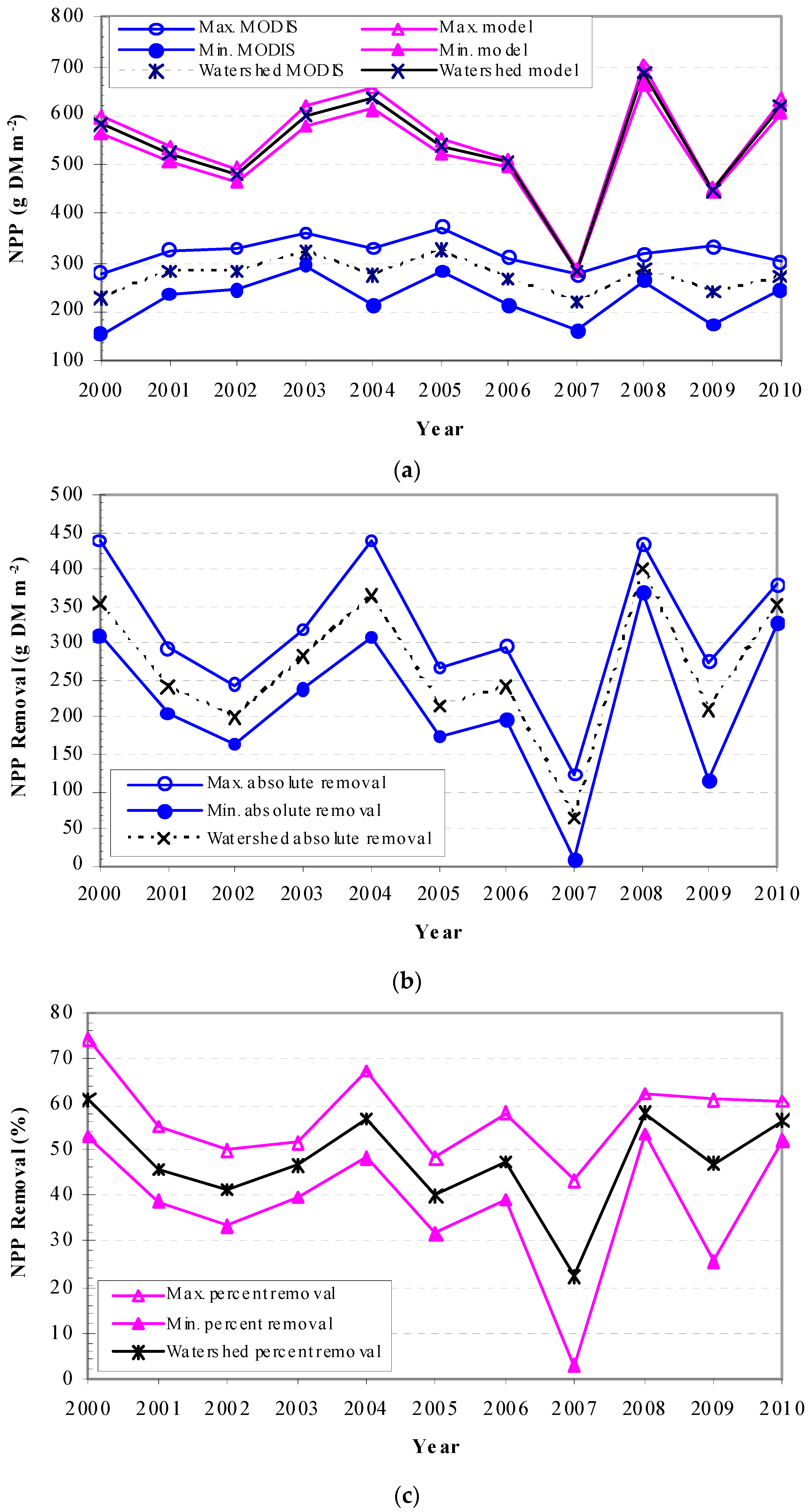
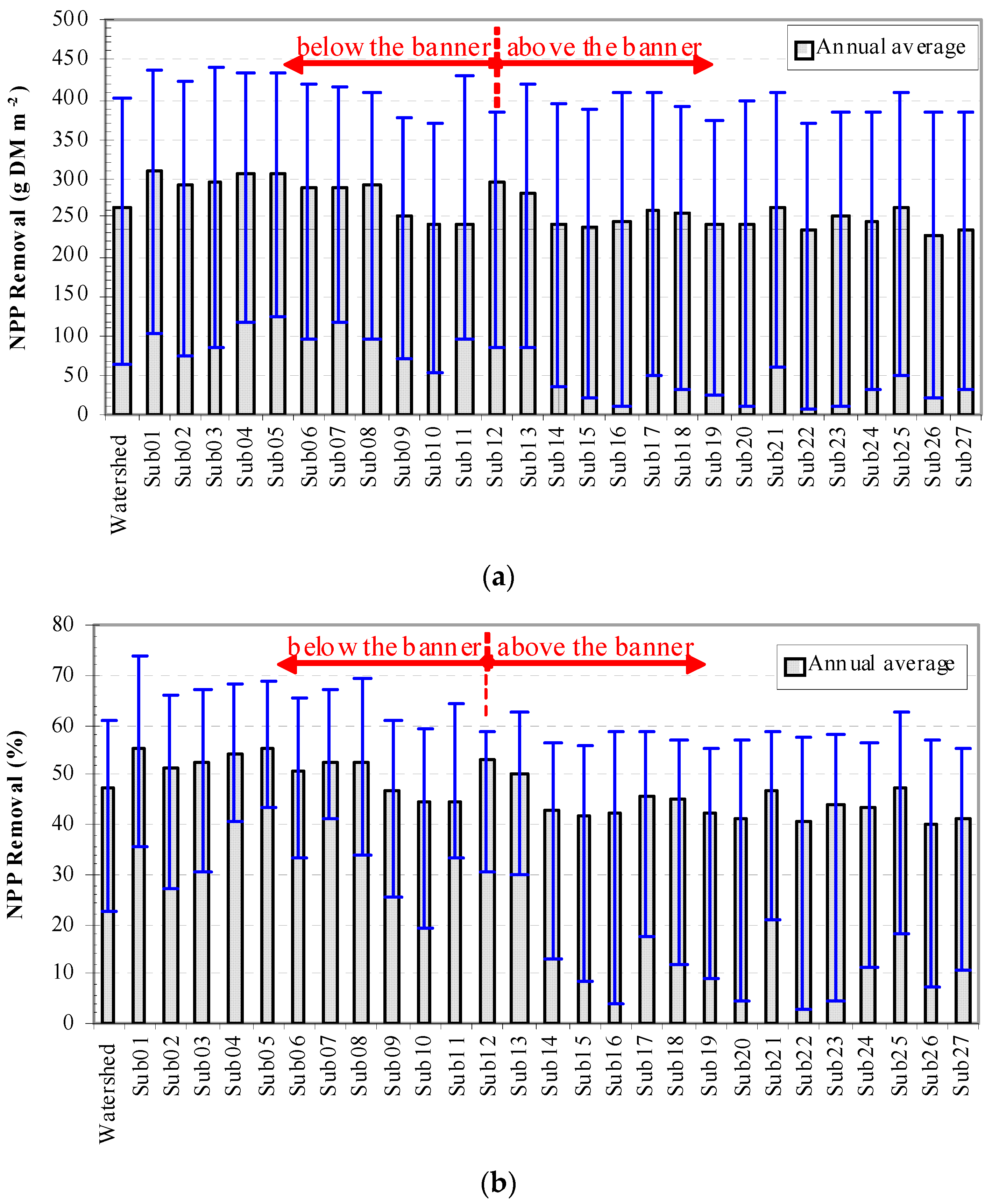
3.2. The Estimated Removal Rate of Grasses

For the study watershed as a whole, the NPP could have varied from 284.7 g DM m⁻² in 2007 to 687.4 g DM m⁻² in 2008 if there were no grazing, whereas the actual NPP was determined to be 220.8 g DM m⁻² in 2007 to 324.7 g DM m⁻² in 2003 (Figure 4a). This indicated that 63.9 to 401.0 g DM m⁻² grasses were grazed (Figure 4b), which is equivalent to 22.4% to 60.9% of the non-grazing grass production (i.e., the predicted natural NPP) (Figure 4c).

Across the study watershed, for a given analysis year, the natural NPP was predicted to be 282.6 g DM m⁻² in one subbasin but as high as 704.0 g DM m⁻² in another subbasin, while the actual NPP was determined to be 161.6 g DM m⁻² in one subbasin but 371.6 g DM m⁻² in another subbasin (Figure 4a). Grazing removed 8.7 to 437.9 g DM m⁻² at the subbasin scales (Figure 5a), which is equivalent to 3.1% to 74.1% of the non-grazing grass production (Figure 5b). Overall, the subbasins downstream of the West Ujimqin banner (near the Baiyingwula flow station shown in Figure 1) had a significantly (p-value = 0.01 < α = 0.05) higher grazing rate than the subbasins upstream of the banner, as indicated by a paired student-t (unequal variances) test [54]. The null hypothesis of the test is that the mean grazing rate of the upper portion of the watershed was not different from the mean grazing rate of the lower portion. However, the grazing rates in the downstream subbasins had a larger variation from year to year than those in the upstream subbasins. The subbasins with maximums and minimums for the analysis years are presented in

Table 2. Subbasins (Figure 1) with maximums and minimums shown in Figure 4 ^†.

Year	Maximums				Minimums
	MODIS-NPP	Model-NPP	Absolute	Percent	MODIS-NPP	Model-NPP	Absolute	Percent
2000	Sub15	Sub20	Sub01	Sub01	Sub01	Sub12	Sub22	Sub15
2001	Sub15	Sub20	Sub01	Sub01	Sub01	Sub12	Sub15	Sub15
2002	Sub20	Sub20	Sub01	Sub01	Sub01	Sub12	Sub20	Sub20
2003	Sub26	Sub20	Sub04	Sub05	Sub08	Sub12	Sub26	Sub26
2004	Sub26	Sub20	Sub03	Sub03	Sub03	Sub12	Sub26	Sub26
2005	Sub15	Sub20	Sub04	Sub04	Sub04	Sub12	Sub15	Sub15
2006	Sub20	Sub20	Sub02	Sub02	Sub02	Sub12	Sub26	Sub26
2007	Sub22	Sub20	Sub05	Sub05	Sub05	Sub12	Sub22	Sub22
2008	Sub22	Sub20	Sub05	Sub01	Sub01	Sub12	Sub10	Sub22
2009	Sub26	Sub20	Sub07	Sub07	Sub07	Sub12	Sub26	Sub26
2010	Sub14	Sub20	Sub01	Sub08	Sub08	Sub12	Sub14	Sub14

Notes: ^† MODIS-NPP: net primary production (NPP) presented by the MODIS images; Model-NPP: NPP predicted by the model (Equations (1) through (11)); Absolute: absolute NPP removal rate by grazing; Percent: percent NPP removal rate by grazing.

.

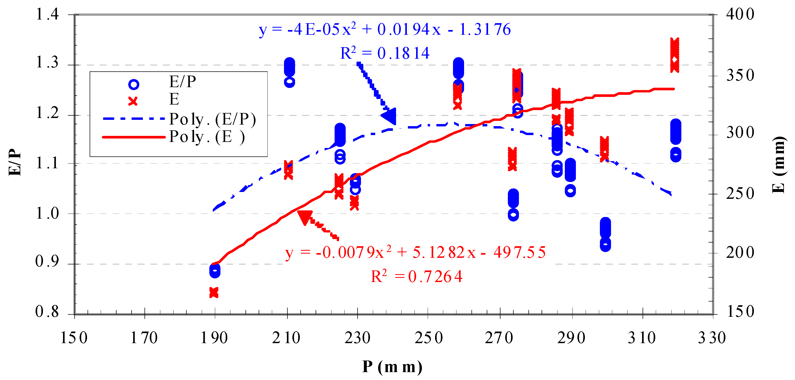
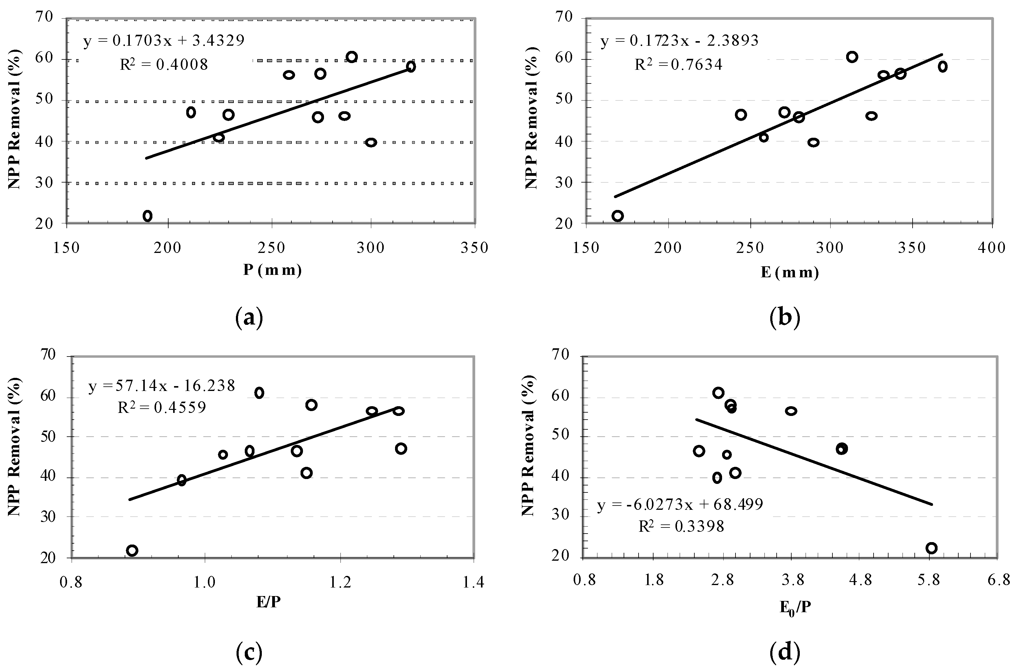
3.3. The Influences of Climate on Grazing Removal Rate of Grasses

The grass removal rate tended to significantly increase with P, E, or $\frac{\mathrm{E}}{\mathrm{P}}$, whereas it tended to marginally decrease with $\frac{{\mathrm{E}}_0}{\mathrm{P}}$ (i.e., atmospheric dryness) (

Table 3. The Pearson correlation coefficients between net primary production (NPP) removal rate and the major climate factors (P: annual precipitation; E: annual actual evapotranspiration; and E₀: annual potential evapotranspiration). The bold coefficients are statistically significant at a significance level of α = 0.05.

Subbasin †	Pearson Correlation Coefficient between NPP Removal Rate (g DM m−2) and				Pearson Correlation Coefficient between NPP Removal Rate (%) and
	P	E	E/P	E0/P	P	E	E/P	E0/P
US 1	0.74	0.96	0.65	−0.64	0.63	0.87	0.68	−0.58
2	0.72	0.92	0.62	−0.64	0.52	0.71	0.55	−0.48
3	0.71	0.94	0.69	−0.62	0.55	0.82	0.72	−0.51
4	0.71	0.94	0.69	−0.62	0.55	0.82	0.72	−0.51
5	0.69	0.93	0.70	−0.60	0.50	0.78	0.71	−0.44
6	0.72	0.93	0.65	−0.59	0.42	0.65	0.55	−0.27
7	0.74	0.94	0.64	−0.61	0.59	0.80	0.61	−0.45
8	0.72	0.90	0.56	−0.55	0.42	0.56	0.38	−0.20
9	0.71	0.93	0.63	−0.60	0.53	0.76	0.60	−0.43
10	0.71	0.93	0.61	−0.57	0.57	0.80	0.60	−0.44
11	0.74	0.96	0.60	−0.64	0.67	0.90	0.63	−0.62
12	0.75	0.95	0.64	−0.62	0.56	0.77	0.60	−0.43
DS 13	0.71	0.94	0.62	−0.58	0.54	0.82	0.63	−0.43
14	0.76	0.96	0.62	−0.68	0.64	0.85	0.61	−0.62
15	0.72	0.95	0.67	−0.62	0.62	0.88	0.71	−0.58
16	0.72	0.96	0.69	−0.62	0.64	0.90	0.74	−0.61
17	0.77	0.97	0.65	−0.67	0.72	0.92	0.68	−0.69
18	0.73	0.96	0.69	−0.62	0.61	0.87	0.72	−0.57
19	0.72	0.96	0.71	−0.64	0.59	0.85	0.74	−0.61
20	0.74	0.96	0.67	−0.65	0.65	0.89	0.70	−0.64
21	0.79	0.97	0.64	−0.70	0.75	0.94	0.67	−0.74
22	0.72	0.95	0.67	−0.62	0.57	0.83	0.69	−0.54
23	0.74	0.96	0.68	−0.66	0.67	0.92	0.71	−0.68
24	0.72	0.97	0.71	−0.69	0.63	0.90	0.75	−0.70
25	0.73	0.96	0.70	−0.67	0.63	0.90	0.75	−0.67
26	0.73	0.94	0.65	−0.63	0.61	0.84	0.66	−0.58
27	0.76	0.95	0.61	−0.66	0.72	0.91	0.63	−0.69
Watershed	0.75	0.96	0.65	−0.67	0.69	0.93	0.70	−0.70

Notes: ^† See Figure 1 for the subbasins. UP: upstream of the City of West Ujimq; DS: downstream of the city.

and Figure 6). A year with a greater $\frac{{\mathrm{E}}_0}{\mathrm{P}}$ is drier, which can restrict vegetation growth resulting in less available grasses for grazing. In contrast, a year with a smaller $\frac{{\mathrm{E}}_0}{\mathrm{P}}$ tends to be wetter, which can increase vegetation growth leading to more available grasses for grazing. Among these four climate factors, E was found to be most positively related to grass production. This is because E reflects the overall natural conditions for vegetation photosynthesis, with a higher E indicating a better condition; and vice versa. In terms of removal rate in percent, the downstream subbasins were less likely influenced by P and $\frac{{\mathrm{E}}_0}{\mathrm{P}}$ than the upstream subbasins, as indicated by that more downstream subbasins have a statistically insignificant Pearson correlation coefficient (Table 3). However, such a contrast between the upstream and downstream subbasins was not found in terms of removal rate in g DM m⁻². This indicates that the downstream subbasins might have a consistently high removal percentage regardless of natural grass production and year (i.e., had a proportionally increased grazing intensity with natural grass production). Herein, it is assumed that grazing intensity and removal rate are positively correlated: a higher grazing intensity corresponds to a larger removal rate, and vice versa. The grazing intensities in the upstream subbasins might have large variations on a yearly basis.

4. Discussion

The method (Equations (1) through (11)) can be parameterized using easily-available data on topography, soil, land use and land cover, and climate. For an area of interest, the method predicts the natural NPP, whereas the MODIS images present the actual NPP. The removal rate can be estimated as the difference of the natural NPP less the actual NPP. In comparison to the conventional survey-based approach, the method is universally applicable and does not require animal-related data (e.g., species and heads). The method can be applied to areas with a small (or large) size and an unknown simple (or complex) grazing pattern. Leriche et al. [53] proposed a model for evaluating the short-term effect of grazing on grass NPP. This model requires inputs of grazing intensity and pattern as well as several other rarely-measured parameters, such as photosynthetically active radiation and ratios of aboveground/belowground to total NPP. Thus, our method can be a more cost-effective tool for any practical efforts in managing, protecting, and/or restoring steppe grasslands, the very important but most beleaguered ecosystems on the planet [1].

The method was applied to the typical-steppe Balagaer River watershed located in northeast China. The results indicate that the evapotranspiration in this arid and semiarid watershed might be enhanced by grass canopy (α_veg = 2.5 > 1) and compensated by soil water (α_sm = 1.15 > 1). This is evidenced by previous studies (e.g., [9,28,55,56] showing that the annual actual evapotranspiration tends to be greater than the annual precipitation most of the years. Precipitation is probably not the sole water source for evapotranspiration. More soil water can be evaporated and transpired on the top of precipitation in a drier than a wetter year. A grass canopy can intercept portion of precipitation, providing more water available for evaporation, while grass roots can uptake soil water, making more water available for transpiration [41]. Overall, the grazing removal rate in the area downstream of the West Ujimqin banner was higher, but had a smaller temporal variation, than that in the area upstream of the banner (Figure 5). The higher removal rate in the downstream area can be attributed to the larger population and thus more grass-grazing animals, whereas the lower removal rate in the upstream area is likely due to the lower population and thus fewer grass-grazing animals (Field reconnaissance by the authors in July 2014; [15]). Another possible reason is that the soils in the upstream area are less saline and more permeable than those in the downstream area, leading to a downstream-to-upstream increase pattern of natural grass production [15]. Averaged across the eleven analysis years, the watershed as a whole had a removal rate of about 47.6%, which is within the global HANPP (human appropriation of net primary production) ranges of 11% to 63% reported by [57]. Here, the only different is that for our study watershed, grazing was the dominant grass removal mechanism, whereas for some other regions (e.g., Sothern Asia and Western Europe), both grazing and harvesting could be the grass removal mechanisms. For an area of interest, when pre-harvest MODIS images are available, our method may be used to better quantify grazing rate in the HANPP calculation, which is needed to quantify the aggregate impact of land use on biomass available each year in ecosystems.

In a previous study in the Balagaer River watershed, Wang et al. [42] conducted a sensitivity analysis of soil erosion to LAI. The take-home result from that analysis was reproduced and is shown in Figure 7 for the convenience of the discussion hereinafter. By assuming that a reference (i.e., an existing) LAI of 0.47 corresponds to the annual average watershed-scale removal rate of 47.6% and that the LAI for a given removal rate can be estimated by Equation (13), the fluvial erosion might not vary much but would be dominated by aeolian erosion (R_a→w > 1 in Figure 7b) during the analysis years. However, a removal rate of higher than 65% would drastically increase the magnitude and risk of soil erosion (steep increasing of R_aw in Figure 7a), and thus can be treated as the threshold for grazing management in the Balager River watershed.

$$\mathrm{LAI}=\frac{1-\left(\mathrm{removalrate}\right)}{1-47.6\%}\times 0.47=\frac{1-\left(\mathrm{removalrate}\right)}{0.524}\times 0.47=0.8969\times \left[1-\left(\mathrm{removalrate}\right)\right]$$

(13)

5. Conclusions

This study presented a method that can be used to estimate grazing removal rate with no requirement of animal-related data (e.g., species and heads). This method assumes that grazing removal rate can be estimated as difference of NPP predicted by a mathematical model less that presented by MODIS. Subsequently, this method was applied to the Balagaer River watershed, which has an arid and semiarid environment and is almost uniformly covered by typical steppe grasses of Leymus chinensis and Stipa grandis. The results indicate that during the eleven analysis years of 2000 to 2010, the watershed had a removal rate ranging from 63.9 to 401.0 g DM m⁻² (or 22.4% to 60.9%). However, across the watershed, the removal rate tended to become larger from the upstream to the downstream. Some subbasins downstream of the West Ujimqin banner were estimated to have a removal rate of up to 437.9 g DM m⁻² (or 74.1%). On the other hand, the removal rate in an upper-side subbasin tended to have a larger temporal variation than that in a lower-side subbasin. At either the watershed or a subbasin scale, the removal rate tended to be larger in a year with larger precipitation (P), actual evapotranspiration (E), and/or $\frac{\mathrm{E}}{\mathrm{P}}$, but it tended to be smaller in a year that was atmospherically drier (i.e., had a greater ratio of annual potential evapotranspiration E₀ to P). For all analysis years, the removal rate of the study watershed was below a threshold of 65%, above which the magnitude and risk of soil erosion (i.e., possible degradation) would be drastically increased. However, for some analysis years, several downstream subbasins might have a removal rate of larger than this threshold and thus could be susceptible to degradation. Our method may be useful in improving the HANPP (human appropriation of net primary production) calculations as well as better managing steppe grasslands all over the world.

References

1. Henwood, W. The world’s temperate grasslands: A beleaguered biome. Parks 1998, 8, 1–2. [Google Scholar]
2. Wang, Z. Strategic considerations for the protection of grassland ecosystems in China. Grassl. China 2005, 27, 1–2. (In Chinese) [Google Scholar]
3. Barnes, R.F.; Nelson, C.J.; Collins, M.; Moore, K.J. Forages: An Introduction to Grassland Agriculture, 6th ed.; Iowa State Press: Ames, IA, USA, 2003; Volume 1. [Google Scholar]
4. Chepil, W.S. Dynamics of wind erosion: V. cumulative intensity of soil drifting across eroding fields. Soil Sci. 1946, 61, 257. [Google Scholar] [CrossRef]
5. Li, B.; Shi, P.J.; Lin, X.Q. Development of a Chinese grassland-livestock balance dynamic monitoring system. Grassl. Sci. 1995, 3, 95–102. [Google Scholar]
6. White, R.P.; Murray, S.; Rohweder, M. Pilot Analysis of Global Ecosystems: Grassland Ecosystems; World Resource Institute: Washington, DC, USA, 2000. [Google Scholar]
7. Intergovernmental Panel on Climate Change (IPCC). Climate Change 2001: The Scientific Basis; Contribution of Working Group 1 to Third Assessment Report of the IPCC (Chairs: J. Houghton and Y. Ding); Cambridge University Press: Cambridge, UK, 2001; p. 881. [Google Scholar]
8. Peart, B. Lift in a Working Landscape: Towards a Conservation Strategy for the World’s Temperate Grasslands. In Proceedings of the Record of the World Temperate Grasslands Conservation Initiative Workshop, Hohhot, China, 28–29 June 2008.
9. Li, S.; Asanuma, J.; Kotani, A.; Davaa, G.; Oyunbaatar, D. Evapotranspiration from a Mongolian steppe under grazing and its environmental constraints. J. Hydrol. 2007, 333, 133–143. [Google Scholar] [CrossRef]
10. Jin, H.; Plaha, P.; Park, J.Y.; Hong, C.P.; Lee, I.S.; Yang, Z.H.; Jiang, G.B.; Kwak, S.S.; Liu, S.K.; Lee, J.S.; et al. Comparative EST profiles of leaf and root of Leymus chinensis, a xerophilous grass adapted to high pH sodic soil. Plant Sci. 2006, 170, 1081–1086. [Google Scholar] [CrossRef]
11. Food and Agriculture Organization of the United Nations (FAO). Crop Evapotranspiration: Guidelines for Computing Crop Water Requirements. 2008. Available online: http://www.fao.org/docrep/x0490e/x0490e08.htm (accessed on 29 August 2014).
12. McCarthy, D.F. Essentials of Soil Mechanics and Foundations, 6th ed.; Prentice Hall: Upper Saddle River, NJ, USA, 2002. [Google Scholar]
13. Wang, X.; Li, F.; Gao, R.; Luo, Y.; Liu, T. Predicted NPP spatiotemporal variations in a semiarid steppe watershed for historical and trending climates. J. Arid Environ. 2014, 104, 67–79. [Google Scholar] [CrossRef]
14. National Meteorological Information Center Website. Available online: http://www.nmic.gov.cn/web/index.htm (accessed on 6 August 2016).
15. Luo, Y.; Wang, X.; Li, F.; Gao, R.; Duan, L.; Liu, T. Responses of grass production to precipitation in a mid-latitude typical steppe watershed. Trans. ASABE 2014, 57, 1595–1610. [Google Scholar]
16. Zhang, X.; Srinivasan, R. GIS-based spatial precipitation estimation using next generation radar and raingauge data. Environ. Model. Softw. 2010, 25, 1781–1788. [Google Scholar] [CrossRef]
17. Ortel, T.; Spies, R. NEXTRAD Quantitative Precipitation Estimates, Data Acquisition, and Processing for the DuPage County, Illinois, Streamflow-Simulation Modeling System; Fact Sheet 2015-3076; U.S. Department of the Interior and U.S. Geological Survey: Washington, DC, USA, 2015.
18. FAO Website. Available online: http://www.iiasa.ac.at/Research/LUC/External-World-Soil-database/HTML (accessed on 6 August 2016).
19. Saxton, K.E.; Rawls, W.J. Soil water characteristic estimates by texture and organic matter for hydrologic solutions. Soil Sci. Soc. Am. J. 2006, 70, 1569–1578. [Google Scholar] [CrossRef]
20. U.S. Geological Survey (USGS). Land Processes Distributed Active Center (LPDAC) Website. Available online: https://lpdaac.usgs.gov/get_data/data_pool (accessed on 6 August 2016).
21. Heinsch, F.A.; Reeves, M.; Votava, P.; Kang, S.; Milesi, C.; Zhao, M.; Glassy, J.; Jolly, W.M.; Loehman, R.; Bowker, C.F.; et al. User’s Guide: GPP and NPP (MOD17A2/A3) Products NASA MODIS Land Algorithm. 2003. Available online: http://www.ntsg.umt.edu/sites/ntsg.umt.edu/files/modis/MOD17UsersGuide.pdf (accessed on 30 June 2016).
22. Guo, X.; He, Y.; Shen, Y.; Feng, D. Analysis of the terrestrial NPP based on the MODIS in the source regions of Yangtze and Yellow Rivers from 2000 to 2004. J. Glaciol. Geocryol. 2006, 28, 512–518. [Google Scholar]
23. Yong, H.; Wenjie, D.; Xiaoyin, G. Terrestrial NPP variation in the region of the South-North Water Diversion Project (East Route). Adv. Clim. Chang. Res. 2006, 2, 246–249. [Google Scholar]
24. He, Y.; Dong, W.; Guo, X.; Dan, L. Terrestrial growth in China and its relationship with climate based on the MODIS data. Acta Ecol. Sin. 2007, 27, 5086–5092. [Google Scholar] [CrossRef]
25. Zhou, G.; Zhen, Y.; Chen, S.; Luo, T. NPP model of natural vegetation and its application in China. Sci. Silvae Sin. 1998, 34, 2–11. (In Chinese) [Google Scholar]
26. Fu, B.P. On the calculation of the evaporation from land surface. Sci. Atmos. Sin. 1981, 5, 23–31. (In Chinese) [Google Scholar]
27. Fu, B.P. On the calculation of evaporation from land surface in mountainous areas. Sci. Atmos. Sin. 1996, 16, 328–335. (In Chinese) [Google Scholar]
28. Zhang, L.; Hickel, K.; Dawes, W.R. A rational function approach for estimating mean annual evaporation. Water Resour. Res. 2004, 40, W02502. [Google Scholar] [CrossRef]
29. Budyko, M.I. The Heat Balance of the Earth’s Surface; National Weather Service, U.S. Department of Commerce: Washington, DC, USA, 1958.
30. Yang, D.; Sun, F.; Liu, Z.; Cong, Z.; Ni, G.; Lei, Z. Analyzing spatial and temporal variability of annual water-energy balance in nonhumid regions of China using the Budyko hypothesis. Water Resour. Res. 2007, 43, W04426. [Google Scholar] [CrossRef]
31. Yang, F.; Zhou, G. Characteristics and modeling of evapotranspiration over a temperate desert steppe in Inner Mongolia, China. J. Hydrol. 2011, 396, 139–147. [Google Scholar] [CrossRef]
32. Istanbulluoglu, E.; Wang, T.; Wright, O.M.; Lenters, J.D. Interpretation of hydrologic trends from a water balance perspective: The role of groundwater storage in the Budyko hypothesis. Water Resour. Res. 2012, 48, W00H16. [Google Scholar] [CrossRef]
33. Hou, Q.; Wang, Y.; Yang, Z.; Shi, G. Dynamic simulation and definition of crop coefficient for typical steppe in Inner Mongolia, China. Chin. J. Plant Ecol. 2010, 34. [Google Scholar] [CrossRef]
34. Wang, X.; Yang, X.; Liu, T.; Li, F.; Gao, R.; Duan, L. Trend and extreme occurrence of precipitation in a mid-latitude Eurasian steppe watershed at various time scales. Hydrol. Process. 2013. [Google Scholar] [CrossRef]
35. Viessman, W. Introduction to Hydrology, 5th ed.; Prentice Hall: Upper Saddle River, NJ, USA, 2002. [Google Scholar]
36. Zhang, L.; Dawes, W.R.; Walker, G.R. Response of mean annual evapotranspiration to vegetation changes at catchment scale. Water Resour. Res. 2001, 37, 701–708. [Google Scholar] [CrossRef]
37. Monteith, J.L. Evaporation and environment. In State and Movement of Water in Living Organisms, Proceedings of the 19th Symposium of the Society of Experimental Biology, New York, NY, USA, 10–15 July 1965; Cambridge University Press: Cambridge, UK, 1965; pp. 205–234. [Google Scholar]
38. Douglas, E.M.; Jacobs, J.M.; Sumner, D.V.; Ray, R.L. A comparison of models for estimating potential evapotranspiration for Florida land cover types. J. Hydrol. 2009, 373, 366–376. [Google Scholar] [CrossRef]
39. Tukimat, N.N.A.; Harun, S.; Shahid, S. Comparison of different methods in estimating potential evapotranspiration at Muda Irrigation Scheme of Malaysia. J. Agric. Rural Dev. Trop. Subtrop. 2012, 113, 77–85. [Google Scholar]
40. Munson, B.R.; Okiishi, T.H.; Huebsch, W.W.; Rothmayer, A.P. Fundamentals of Fluid Mechanics; John Wiley & Sons, Inc.: Hoboken, NJ, USA, 2012. [Google Scholar]
41. Brutsaert, W. Hydrology: An Introduction; Cambridge University Press: West Nyack, NY, USA, 2005. [Google Scholar]
42. Wang, X.; Liu, T.; Li, F.; Gao, R.; Yang, X.; Duan, L.; Luo, Y.; Li, R. Simulated soil erosion from a semiarid typical steppe watershed using an integrated aeolian and fluvial prediction model. Hydrol. Process. 2014, 28, 325–340. [Google Scholar] [CrossRef]
43. Irmak, S.; Irmak, A.; Jones, J.W.; Howell, T.A.; Jacobs, J.M.; Allen, R.G.; Hoogenboom, G. Predicting daily net radiation using minimum climatological data. J. Irrig. Drain. Eng. 2003, 129, 256–269. [Google Scholar] [CrossRef]
44. Van Genuchten, M.T. A closed-form equation for predicting the hydraulic conductivity of unsaturated soils. Soil Sci. Soc. Am. J. 1980, 44, 892–898. [Google Scholar] [CrossRef]
45. Ghanbarian-Alavijeh, B.; Liaghat, A.; Huang, G.; van Genuchten, M.T. Estimation of the van Genuchten soil water retention properties from soil textural data. Pedoshere 2010, 20, 456–465. [Google Scholar] [CrossRef]
46. Saxton, K.E.; Rawls, W.J.; Romberger, J.S.; Papendick, R.I. Estimating generalizaed soil-water characteristics from texture. Trans. ASAE 1986, 50, 1031–1035. [Google Scholar]
47. Allen, R.G.; Pereira, L.S.; Smith, M.; Raes, D.; Wright, J.L. FAO-56 Dual Crop Coefficient method for estimating evaporation from soil and application extensions. J. Irrig. Drain. Eng. 2005, 131, 2–13. [Google Scholar] [CrossRef]
48. Liu, Y.; Luo, Y. A consolidated evaluation of the FAO-56 dual crop coefficient approach using the lysimeter data in the North China Plain. Agric. Water Manag. 2010, 97, 31–40. [Google Scholar] [CrossRef]
49. Li, L.; Liu, X.; Chen, Z. Study on the carbon cycle of Leymus Chinensis steppe in the Xilin River Basin. Acta Bot. Sin. 1998, 40, 955–961. [Google Scholar]
50. Schönbach, P.; Wan, H.; Gierus, M.; Bai, Y.; Müller, K.; Lin, L.; Susenbeth, A.; Taube, F. Grassland responses to grazing: Effects of grazing intensity and management system in an Inner Mongolian steppe ecosystem. Plant Soil 2011, 340, 103–115. [Google Scholar] [CrossRef]
51. Ren, H.; Schönbach, P.; Wan, H.; Gienus, M.; Taube, F. Effects of grazing intensity and environmental factors on species composition and diversity in typical steppe of Inner Mongolia, China. PLoS ONE 2012, 7, e52180. [Google Scholar] [CrossRef] [PubMed]
52. Yan, L.; Zhou, G.; Zhang, F. Effects of different grazing intensities on grassland production in China: A meta-analysis. PLoS ONE 2013, 8, e81466. [Google Scholar] [CrossRef] [PubMed]
53. Leriche, H.; LeRoux, X.; Gignoux, J.; Tuzet, A.; Fritz, H.; Abbadie, L.; Loreau, M. Which functional processes control the short-term effect of grazing on net primary production in grasslands? Oecologia 2001, 129, 114–124. [Google Scholar]
54. Neter, J.; Kutner, M.H.; Nachtsheim, C.J.; Wasserman, W. Applied Linear Statistical Models, 4th ed.; McGraw-Hill Companies, Inc.: New York, NY, USA, 1996. [Google Scholar]
55. Zhou, G.; Wang, Y.; Wang, S. Responses of grassland ecosystems to precipitation and land use along the northeast China transect. J. Veg. Sci. 2002, 13, 361–368. [Google Scholar] [CrossRef]
56. Hao, Y.; Wang, Y.; Mei, X.; Huang, X.; Cui, X.; Zhou, X.; Niu, H. CO2, H2O and energy exchange of an Inner Mongolia steppe ecosystem during a dry and wet year. Acta Oecol. 2008, 33, 133–143. [Google Scholar] [CrossRef]
57. Haberl, H.; Erb, K.H.; Krausmann, F.; Gaube, V.; Bondeau, A.; Plutzar, C.; Gingrich, S.; Lucht, W.; Fischer-Kowalski, M. Quantifying and mapping the human appropriation of net primary production in earth’s terrestrial ecosystems. Proc. Natl. Acad. Sci. USA 2007, 104, 12942–12947. [Google Scholar] [CrossRef] [PubMed]
Figure 1. Map showing the location, soils (i.e., World Food and Agriculture Organization or FAO soil classes), boundary, and subbasins of the Balagaer River watershed.
Water 08 00339 g001
Figure 2. Typical steppe grasses (e.g., Leymus chinensis and Stipa grandis) in the Balagaer River watershed.
Water 08 00339 g002
Figure 3. Plot showing ratio of annual actual evapotranspiration (E) to annual precipitation (P), as well as E, versus P.
Water 08 00339 g003
Figure 4. Plots showing the: (a) MODIS-presented and model-predicted net primary production (NPP); (b) absolute NPP removal rate by grazing; and (c) percent removal rate, versus year.
Water 08 00339 g004
Figure 5. Plots showing the annual average and the minimum and maximum (error bars) of: (a) net primary production (NPP); and (b) NPP removal rate, for the study watershed as a whole and the 27 subbasins. Herein, the “banner” refers to the City of West Ujimqin, which is in the vicinity of the Baiyingwula flow station shown in Figure 1.
Water 08 00339 g005
Figure 6. Plots showing net primary production (NPP) removal rate versus: (a) annual precipitation (P); (b) annual actual evapotranspiration (E); (c) E/P; and (d) atmospheric dryness (defined as the ratio of annual potential evapotranspiration E0 to P).
Water 08 00339 g006
Figure 7. Sensitivity of soil erosion to leaf area index (LAI) as influenced by soil moisture for: (a) total erosion Raw; and (b) aeolian in relative to fluvial erosion Ra→w. The definitions and formularizations of Raw and Ra→w can be found in [42].
Water 08 00339 g007