Assessment of the Impact of Subsurface Agricultural Drainage on Soil Water Storage and Flows of a Small Watershed

Abstract

3D hydrological modeling was performed, using CATHY (acronym for CATchment HYdrology model), with the basic objective of checking whether the model could reproduce the effects of subsurface agricultural drainage on stream flows and soil water storage. The model was also used to further our understanding of the impact of soil hydrodynamic properties on watershed hydrology. Flows simulated by CATHY were consistent with traditional subsurface drainage approaches and, for wet years, flows at the outlet of the study watershed corroborated well with observed data. Temporal storage variation analyses illustrated that flows depended not only on the amount of rainfall, but also on its distribution throughout the year. Subsurface agricultural drainage increased base and total flows, and decreased peak flows. Hydrograph separation using simulated results indicated that exfiltration was the most dominant process; peak flows were largely characterized by overland flow; and subsurface drain flow variations were low.

1. Introduction

Subsurface drainage is a common agricultural practice to improve aeration and trafficability of soils in regions characterized by seasonal high water tables [1,2]. Subsurface drainage system helps to increase crop yield of poorly drained soils by providing a better environment for plant growth, especially during wet periods [3] and improve field conditions for timely tillage, planting and harvesting [4,5].

When subsurface drains are in place, the drainable water fraction of the soil profile is converted to short-term (detention) storage over a period of few hours, days, or weeks, depending on a number of variables [6]. These include subsurface drain size, depth and spacing, soil type, outlet size/condition, and whether or not under continuous rainfall or snowmelt conditions. When drainable water is removed from the soil profile, infiltration can then occur. This is due to available soil pore space allowing water that would otherwise be stored in the surface depressions to infiltrate and have a direct pathway to downstream flow via the subsurface drains [6].

Although agricultural production has benefited from agricultural drainage in many regions and countries, there are concerns about potential environmental impacts [7]. The most dramatic hydrological changes in a landscape occur when the latter is converted from native vegetation to intensive cropping systems. When tile drains are implemented, they can substantially alter the total water yield from a field or small watershed as well as modify the timing and shape of the hydrograph [8]. Tile drainage increases the proportion of annual precipitation that is discharged to surface waters via subsurface flow relative to the amount that is stored, evaporated or transpired [9,10,11].

From several studies across the Midwestern United States and Canada, discharge from subsurface drains constitutes the majority of stream flow in many agricultural watersheds. It was found that tile drainage contributed 51% of annual stream flow in a headwater watershed in Ohio [12]. Meanwhile, in a watershed in Ontario, Canada, it was estimated that 42% of annual watershed discharge originated from subsurface drain flow [13]. Culley and Bolton [14] and Xue et al. [15] also estimated that 60% and 86%, respectively, of stream flow was derived from tile drain. Although total water yield from a field tends to increase following installation of subsurface drainage, surface runoff and sediment yields are often significantly decreased [2,16,17]. Subsurface drainage reduces both peak outflows and the frequency of surface runoff events at sites characterized by high water tables or prolonged surface saturation (“ponding”) under undrained conditions [16,18].

The main water quality concern about subsurface drainage is the increased loss of nitrates and other soluble constituents (i.e., pesticides and dissolved phosphorus, to name a few) that can move through soils and end up in nearby surface waters. Meanwhile, it is generally agreed that, through the installation of subsurface drainage, the amount of particulate phosphorus and soil transported by surface runoff is decreased because the volume of surface runoff is reduced [19,20]. However, dissolved phosphorus loss via artificial drainage has been shown to contribute to the accelerated eutrophication of rivers, lakes, estuaries and even coastal waters, including some of the most challenging cases of agriculturally-derived eutrophication [21]. On more permeable soils, where infiltration, soil water storage capacity, and lateral conductivity/seepage is large enough to handle a given storm event, subsurface drainage may have the opposite effect for an event of equivalent magnitude, increasing peak flows by increasing the speed of subsurface discharges [18,22]. In fields where diffuse pollution dominates, installation of artificial drainage can increase peak flows, which accounts for the majority of phosphorus loss, and hence can improve the hydrological connectivity of otherwise isolated areas of the landscape [23,24]. Increased peak flows due to agricultural tile drainage have also been shown to increase channel widening and bank erosion [25].

The impact of artificial drainage strongly depends on characteristics of an individual site, including: topography (slope), drainage system design (spacing, depth and size of drains) as well as soil type (hydraulic conductivity) [26,27]. The hydrological response of subsurface drainage during a given event varies based on event characteristics, such as rainfall amount and intensity [28], and antecedent soil moisture conditions [13,17,29]. Therefore, there is a need for research to better understand the impact of subsurface drainage at both field scale and catchment scale.

The goal of this study was, using a coupled surface water groundwater hydrological model, to quantify the impact of subsurface agricultural drainage and soil properties on the hydrologic functioning of a micro-watershed under intensive farming of annual crops such as grain corn (Zea mays) or soybean (Glycine max). The specific objectives of this study were: (1) to simulate the micro-watershed outlet flow and analyse the effect of subsurface agricultural drainage on soil water storage variation; and (2) to analyse the impact of drainage networks and soil saturated hydraulic conductivity on: (2a) micro-watershed outlet flow; (2b) surface runoff, surface water and groundwater coupling; and (2c) micro-watershed outlet flow hydrograph.

To our knowledge, although there are studies dealing with testing (evaluation) and application of the coupled surface water groundwater hydrological model used in this study, CATHY (acronym for CATchment HYdrology) [30,31,32,33,34,35,36,37,38,39,40,41,42,43], there are no exhaustive studies investigating the influence of artificial subsurface drainage on flows at the watershed level. CATHY is the type of process-based model that is required to study the spatio-temporal variability of soil moisture, groundwater flow and surface runoff. Furthermore, as a virtual laboratory, CATHY provides a powerful deterministic approach to further our understanding of the impact of subsurface drainage on stream flow.

In this respect, not only does this study make a significant contribution to the understanding of CATHY, but it is also the first investigation dealing with the impact of subsurface agricultural drains on the partitioning of flow at a watershed outlet using a 3D model.

2. Materials and Methods

2.1. Study Site

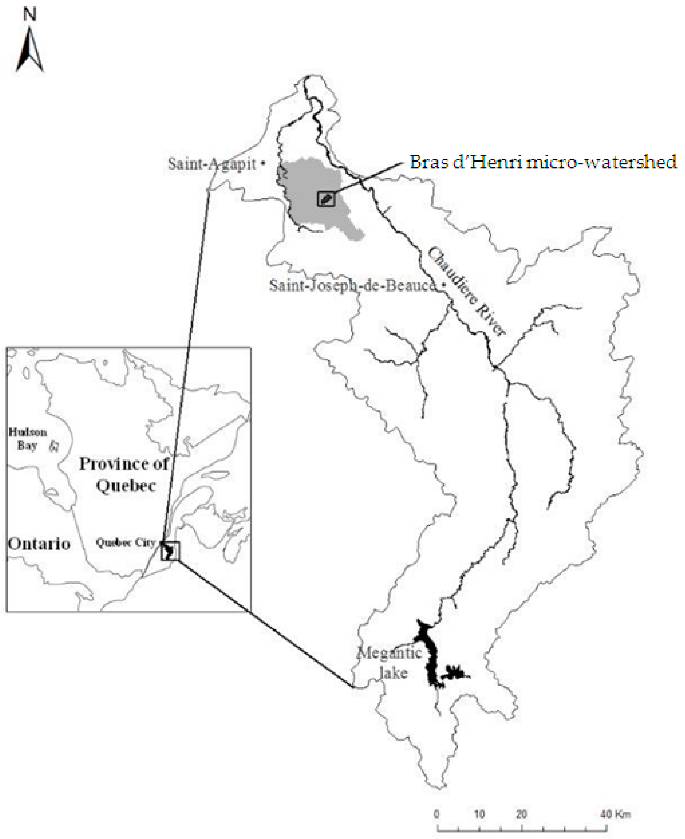
The study site is a micro-watershed of 2.4 km² with latitude and longitude of 46°29′00″ N and 71°14′00″ W, respectively, located in the watershed of the Bras d’Henri River which covers approximately 167 km², a sub-watershed of the Beaurivage River. The latter is located about 30 km southeast of Quebec City on the south shore of the Saint Lawrence River, within the Chaudière-Appalaches agro-climatic region (Figure 1). Two-thirds of this drainage area is currently dedicated to agriculture (large-scale farming, pastures, etc.) while the balance remains in its natural state, which includes wooded areas and wetlands.

The region is characterized by long and cold winters, short and cool summers, and significant annual precipitation, approximately 1150 mm/year, a third of which accumulates as snow. During the summer, precipitation is generally greater than the amount of water lost to evapotranspiration. Thus, no water deficit is observed at soil level, except for a slight possibility in certain sectors of coarse sandy soil with gravel and stones which drains well to very rapidly from the plain and this exclusively during the month of July [44]. The site is covered by the “Watershed Evaluation of Beneficial Management Practices (WEBs)” program, launched nationally in 2004 and managed by Agriculture and Agri-Food Canada (AAC), which aims at measuring the environmental and economic impact of certain Beneficial Management Practices (BMPs) on the quality of water in seven hydrographic micro-watersheds in Canada [45,46,47].

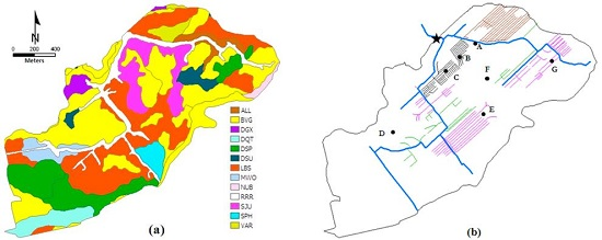
The site is characterized by intensive agricultural production composed essentially of silage (53.1%), grain corn (Zea mays, 27.8%) and soybean (Glycine max, 8.1%). Figure 2a shows the soil codes of the different soil families from the surface to a depth of 1.25 m while the

Table 1. Different families of soil and their percentage of sand, silt and clay.

Soil Code	Soil Family	Sand (%)	Silt (%)	Clay (%)
BVG	Sandy	67–97	2–28	1–13
SJU	Fine sandy loam	68–94	4–31	1–4
VAR	Fine sandy loam	73–97	2–21	1–6
SPH	Silt loam	55–76	22–41	2–5
DGX	Coarse loamy	29–59	34–60	5–13
DSU	Coarse loamy	45–62	33–43	5–12
NUB	Loamy	8–60	33–64	7–32
LBS	Loamy	9–30	58–73	12–23
DQT	Coarse loamy	64–84	7–19	9–20
DSP	Coarse loamy	52–58	33–42	6–10
MWO	Coarse loamy	57–84	10–27	6–17
ALL	Loamy	45–62	33–43	5–12
RRR	Not classified	7–30	58–73	12–23

gives their names and percentage of sand, silt and clay. The corresponding geometric means of the soil saturated hydraulic conductivities are given in

Table 2. Saturated hydraulic conductivity values (K_s), in m/s, and their geometric mean of the different soil families up to depth of 1.25 m.

Soil Code	Soil Profile (cm)
	0–25	25–50	50–75	75–100	100–125
BVG00	5.44 × 10−5	1.91 × 10−5	2.94 × 10−4	1.78 × 10−4	1.78 × 10−4
BVG49	2.78 × 10−5	9.03 × 10−5	1.39 × 10−4	1.39 × 10−4	1.39 × 10−4
SJU	9.03 × 10−6	9.03 × 10−5	9.03 × 10−5	9.03 × 10−6	9.03 × 10−6
VAR	8.42 × 10−6	8.11 × 10−5	9.75 × 10−5	8.11 × 10−5	8.11 × 10−5
SPH	5.44 × 10−5	1.91 × 10−5	2.94 × 10−4	1.78 × 10−4	1.78 × 10−4
DGX	2.43 × 10−5	1.70 × 10−5	1.39 × 10−7	1.39 × 10−7	1.39 × 10−7
DSU	1.39 × 10−7	2.22 × 10−7	1.39 × 10−7	2.78 × 10−8	2.78 × 10−8
NUB	5.56 × 10−6	1.42 × 10−6	1.39 × 10−7	1.39 × 10−7	1.39 × 10−7
LBS	8.06 × 10−7	1.04 × 10−5	8.33 × 10−8	1.39 × 10−7	1.39 × 10−7
DQT	1.31 × 10−4	1.25 × 10−4	2.73 × 10−4	2.66 × 10−4	2.66 × 10−4
DSP	3.06 × 10−7	1.21 × 10−5	2.31 × 10−6	4.44 × 10−7	4.44 × 10−7
MWO	5.86 × 10−5	6.00 × 10−5	1.36 × 10−4	1.95 × 10−5	1.95 × 10−5
ALL	1.39 × 10−7	2.22 × 10−7	1.39 × 10−7	2.78 × 10−8	2.78 × 10−8
RRR	2.78 × 10−6	2.78 × 10−6	2.78 × 10−6	2.78 × 10−6	2.78 × 10−6
Geometric mean of Ks	6.04 × 10−6	1.16 × 10−5	7.07 × 10−6	3.51 × 10−6	3.51 × 10−6

. The location of the drainage systems (at a depth of 1.20 m and occupying 30% of the total area of the watershed) is presented in Figure 2b.

2.2. Data Source

The database provided by AAC includes meteorological data (average air temperature, relative humidity, saturated vapour pressure, wind speed at an altitude of 2 m, net radiation, precipitation, etc.), saturated hydraulic conductivity of soils up to a depth of 1.25 m obtained from suction tests, and water height data measured every 15 min at the outlet of the micro-watershed by a probe installed above the stream. The water flow rate data were obtained by means of calibration curves (linking flow rate to water height) determined by Ratté-Fortin [49].

The saturated hydraulic conductivities of the soil at a depth greater than 1.25 m were obtained from permeability tests or slug tests [50,51] conducted at the piezometer locations identified in Figure 2b. The saturated hydraulic conductivity values varied from 3.33 × 10⁻⁶ to 2.08 × 10⁻⁵ m/s with a geometric mean of 1.29 × 10⁻⁵ m/s.

Given the number of soil families and piezometers, the saturated hydraulic conductivity value of each horizon of the soil profile was used to calibrate the hydrological model, the geometric means of each horizon being used as initial values.

2.3. The CATHY Model

CATHY is a spatially-distributed physics-based model that integrates surface and subsurface flows [52]. The surface flow (in rills and waterway) is generally formulated by the Saint Venant equation:

$$\frac{\partial Q}{\partial t}+C_k\frac{\partial Q}{\partial s}=D_h\frac{{\partial }^{2}Q}{\partial s^2}+C_k{q}_s$$

(1)

This equation is resolved numerically by the finite difference method. Since the CATHY model is a rill flow-based model, Equation (1) is represented in a 1D coordinate system s (L) to describe each element of the surface drainage network, where Q is the flow rate along the rivulet/waterway (L³/T), $C_k$ is the kinematic celerity (L/T), $D_h$ is the hydraulic diffusivity (L²/T), and $q_s$ is the input flow rate (positive) in the medium or the output flow rate (negative) from the subsurface to the surface (L³/LT).

Richards 3D equation (Equation (2)), which describes flow in a variably-saturated media (subsurface flow), is resolved numerically in space by the Galerkin finite element method using tetrahedral elements. Since the storage and conductivity terms strongly depend on pressure, Equation (2) is mostly nonlinear and, as a result, is linearized by Picard’s or Newton’s iterative methods [53]. Thus, the partial differential equation, which mathematically describes the flow in porous media, is:

$$S_w{S}_s\frac{\partial \psi }{\partial t}+\varphi \frac{\partial S_w}{\partial t}=\nabla .\left[K_s{K}_r\left(\nabla \psi +{\eta }_z\right)\right]+q_{ss}$$

(2)

where $S_w=\theta /{\theta }_s$ is the saturation level, $\theta$ is the volumetric water content (-), ${\theta }_s$ is the saturated water content (generally equal to the porosity $\varphi$), $S_s$ is the specific storage coefficient (1/L), $\psi$ is the capillary potential (L), t is time (T), ∇ is the gradient operator, $K_s$ is the hydraulic conductivity tensor (LT), $K_r\left(\psi \right)$ is the relative conductivity function (-), ${\eta }_z={\left(0,0,1\right)}^T$, z is the vertical coordinate oriented towards the top (L), and $q_{ss}$ represents the source (positive) or the well (negative) (L³/L³T).

CATHY is a complex hydrological model with different and varied advantages. The surface hydrology links terrain topography, hydraulic geometry and flow dynamics. Its outputs include surface pressure head (or ponding), overland fluxes, subsurface pressure head and moisture content values, and groundwater velocities. Numerous other variables can be derived from these main outputs such as aquifer recharge, catchment saturation, and stream flow. Surface and subsurface contributions to runoff can be computed at any specified surface node within the catchment, and by default also at the catchment outlet, representing the total stream flow at the outlet.

As a robust model, the use of CATHY requires many input data (parameters). In its current version, no dimension of diameter or radius is taken in account regarding the tile-drain representation in the subsurface porous medium.

To our knowledge, there has not been any study involving CATHY and dealing with the equifinality thesis (identifiability of equally-performing sets of parameter values) or estimation of uncertainty. To our knowledge, all reported papers on CATHY have shown that the model has always been calibrated using observed parameter values mainly of soil saturated hydraulic conductivity and soil porosity. This is mostly a result of the large computational time required to run CATHY as reported in our global sensitivity analysis of the model [48]. It is in this deterministic context that this study was conducted rather than an underestimation of parameter uncertainties.

The subsurface drainage system is represented in the model by assigning a pressure potential (Dirichlet boundary condition) or a flux (Neumann boundary condition) to the corresponding node. More detailed descriptions of the model can be found in the work of Camporese et al. [52].

2.4. Setting up CATHY at the Watershed Scale

2.4.1. Discretization of the Porous Medium

The application of CATHY was developed on the micro-watershed using a Digital Elevation Model (DEM) with a resolution of 20 m. The porous medium was discretized into 15 layers with thinner layers at the surface and near the nodes located closest to the drainage networks at a depth of 1.20 m (interface of the 7th and 8th layers). This was done to properly account for the interactions between surface and subsurface waters and for the influence of drains on the flow. The discretization of the watershed surface resulted in 6148 cells; each one divided into 2 triangles, producing 12,296 cells (linked by 6391 nodes). The latter cells were projected vertically on the 15 layers with each triangle creating three tetrahedrons. The porous medium was thus represented by 553,320 (12,296 × 3 × 15) tetrahedral elements linked by 102,256 nodes (6391 × (15 + 1)).

The values of the soil hydrodynamic properties, that is the saturated soil hydraulic conductivity in the horizontal (in X and Y, or KsXY) and vertical (KsZ) planes, the specific storage coefficient (Ss), and the porosity (φ), associated with each layer of the porous medium are introduced in

Table 3. Soil hydraulic properties of the porous medium for Scenario 1 (corrugated line between layers 7 and 8 indicating the location of drainage network nodes in the drained parcels.

Layer Number	ΔZ (m)	Z (m)	KsXY (m/s)	KsZ (m/s)	Ss (m−1)	φ (-)
01	0.10	0.10	6.06 × 10−5	6.06 × 10−6	3.75 × 10−3	0.52
02	0.15	0.25
03	0.25	0.50	3.80 × 10−4	3.80 × 10−5	1.15 × 10−3	0.48
04	0.25	0.75	4.04 × 10−5	4.04 × 10−6	3.75 × 10−3	0.37
05	0.25	1.00	6.06 × 10−5	6.06 × 10−6	3.75 × 10−3	0.48
06	0.10	1.10
07	0.10	1.20
08	0.10	1.30
09	0.30	1.60	4.20 × 10−4	4.20 × 10−5	1.15 × 10−3	0.50
10	0.45	2.05
11	0.50	2.65
12	0.60	3.26
13	0.64	3.90
14	0.70	4.60
15	0.85	5.45

. In the vertical direction, there are 5 groups of layers: the first group includes layers 1 and 2, the second group layer 3, the third group layer 4, the fifth group layers 5 to 8 (location of the drainage networks), and the fifth group layers 9 to 15 as a whole. The first two layers make up the superior or surface layer where the partition of available water (precipitation) into surface water and infiltration takes place, as well as the superficial transfer.

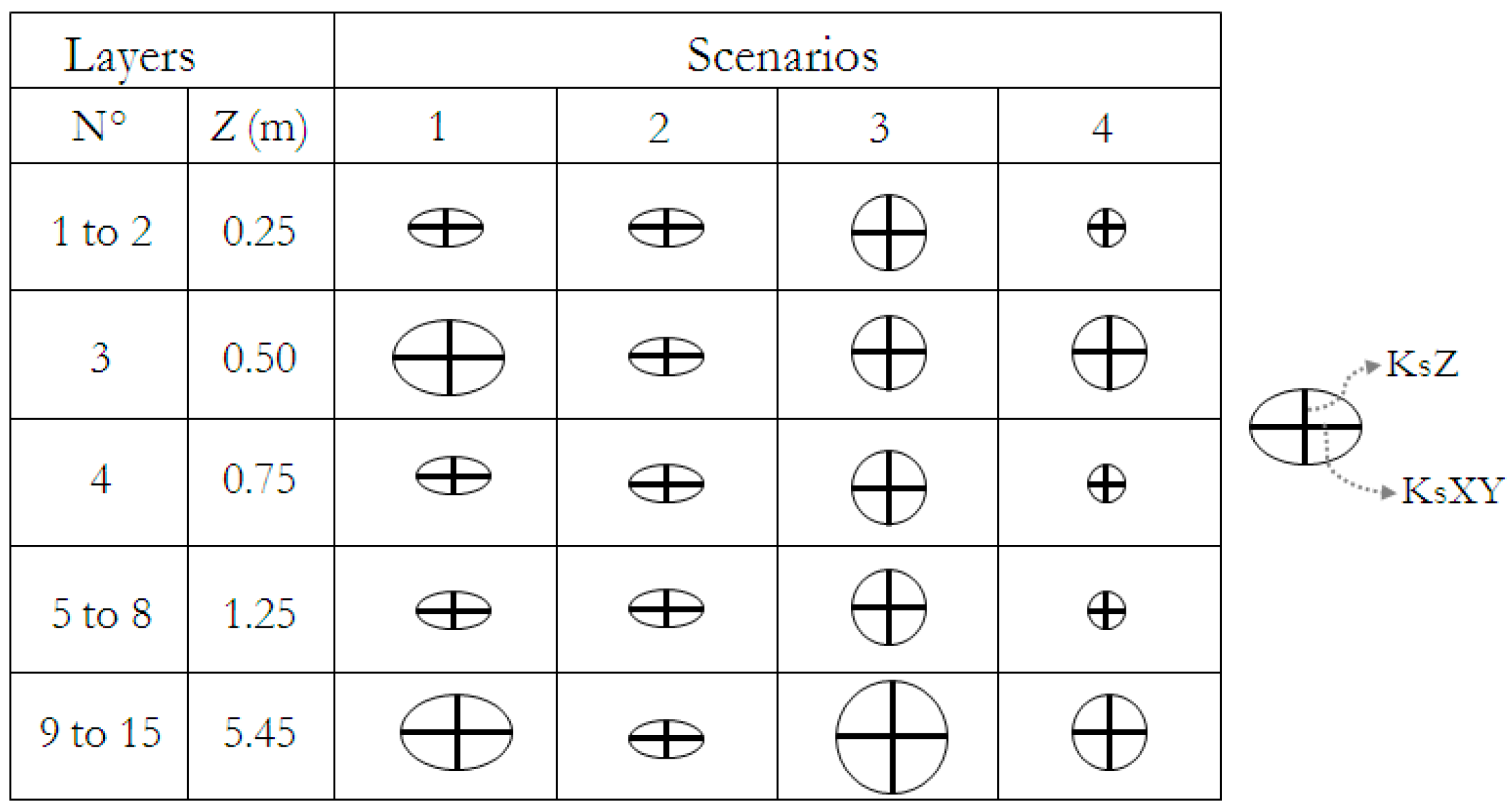
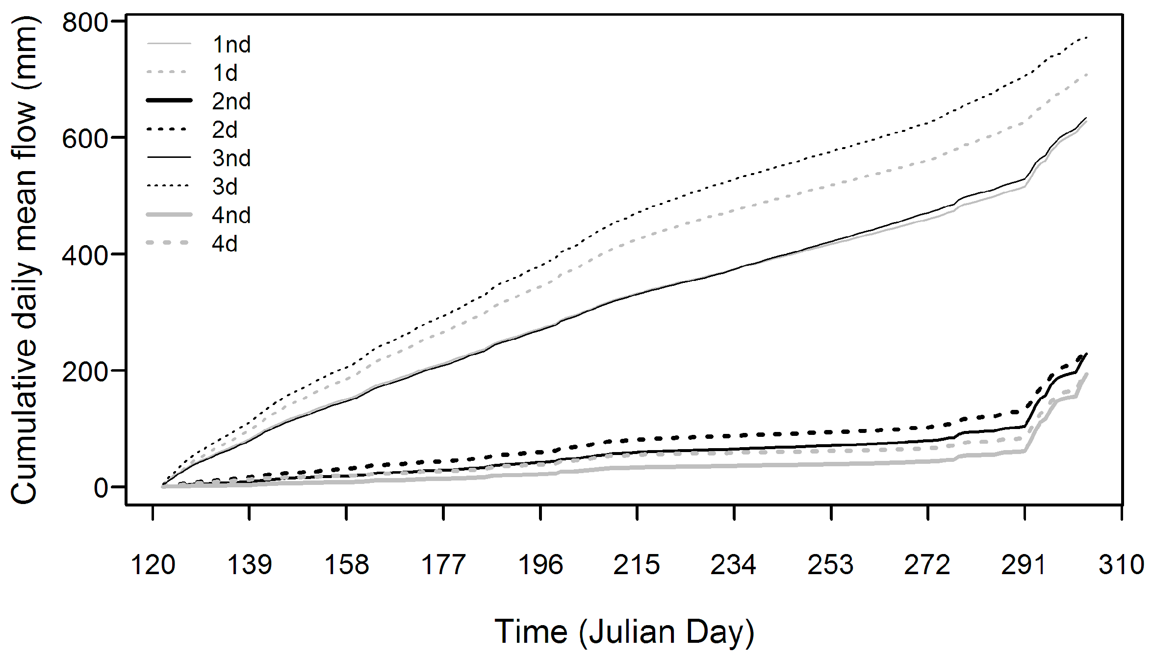
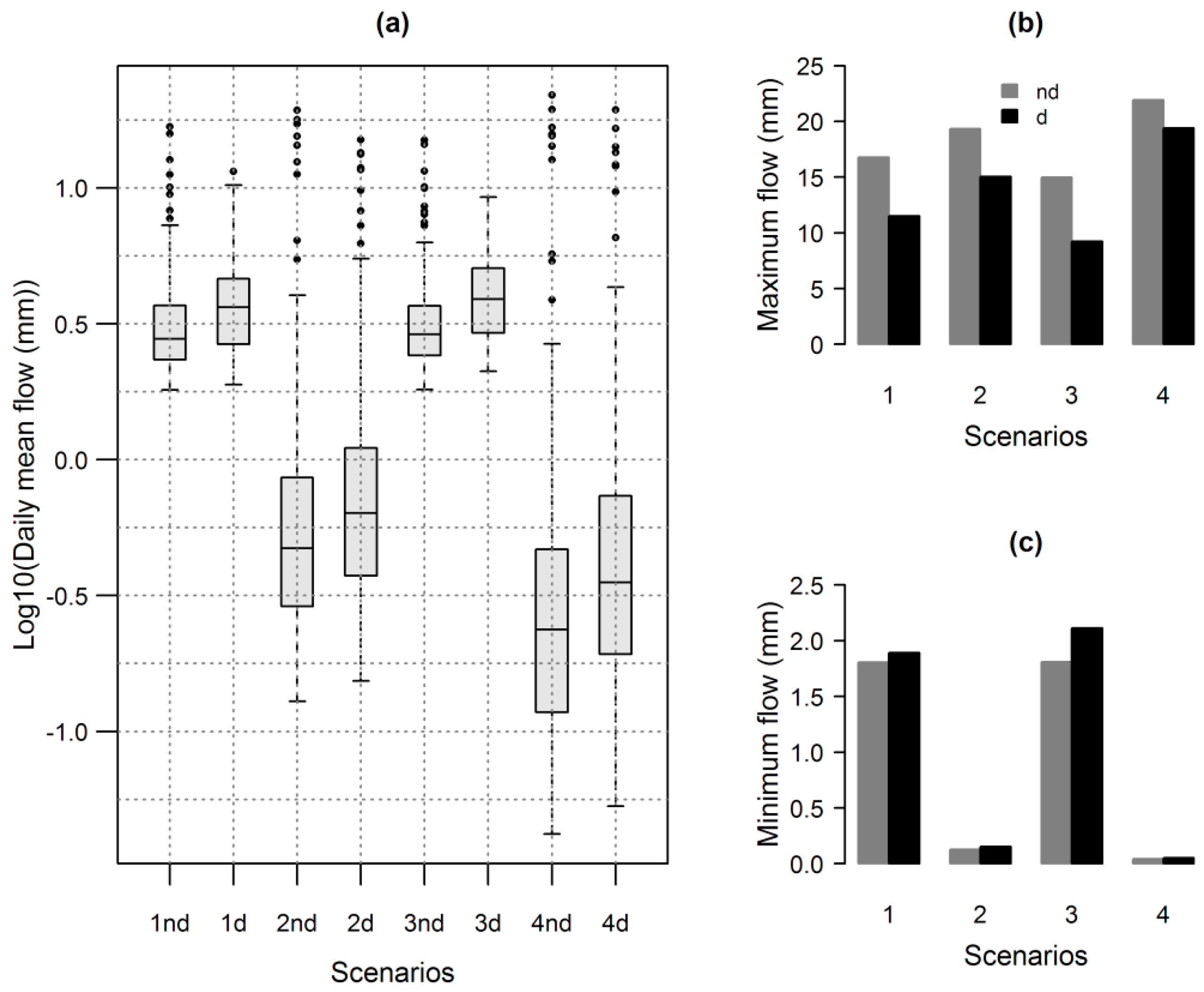
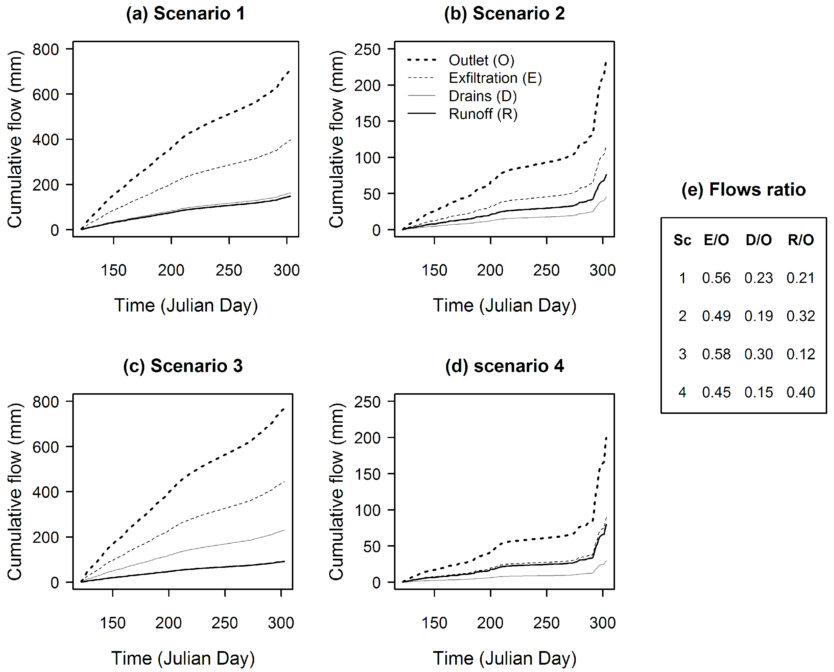
In this study, four scenarios of saturated hydraulic conductivity values were used. The first scenario (Sc. 1), considered as the baseline scenario, is a non-homogenous medium with anisotropic values in each group of layers as given in Table 3 and derived from measured saturated hydraulic conductivity values. They were used to calibrate (saturated hydraulic conductivity was the parameter mostly adjusted during this process) and validate the model. In order to analyse the impact of drainage networks and soils on: (a) the flow at the outlet of the micro-watershed; (b) the coupling of surface water and groundwater, and surface runoff; and (c) the hydrograph at the outlet of the micro-watershed, in addition to the baseline scenario, three additional values of saturated hydraulic conductivity were taken into account based on the fact that, when measuring the saturated hydraulic conductivities in situ or in laboratory, their values can fluctuate within a certain range of order 10 (

Table 4. Isotropic and anisotropic properties of soil saturated hydraulic conductivity (*) analysed.

Layers			Scenarios
N°	ΔZ (m)	Z (m)	1 (Reference)	2	3	4
01	0.10	0.25	$6.06\times {10}^{-5}/6.06\times {10}^{-6}$	$6.06\times {10}^{-5}/6.06\times {10}^{-6}$	$6.06\times {10}^{-5}/6.06\times {10}^{-5}$	$6.06\times {10}^{-6}/6.06\times {10}^{-6}$
02	0.15
03	0.25	0.50	$3.80\times {10}^{-4}/3.80\times {10}^{-5}$			$3.80\times {10}^{-5}/3.80\times {10}^{-5}$
04	0.25	0.75	$4.04\times {10}^{-5}/4.04\times {10}^{-6}$			$4.04\times {10}^{-6}/4.04\times {10}^{-6}$
05	0.25	1.30	$6.06\times {10}^{-5}/6.06\times {10}^{-6}$			$6.06\times {10}^{-6}/6.06\times {10}^{-6}$
06	0.10
07	0.10
08	0.10
09	0.30	5.45	$4.20\times {10}^{-4}/4.20\times {10}^{-5}$		$4.20\times {10}^{-4}/4.20\times {10}^{-4}$	$4.20\times {10}^{-5}/4.20\times {10}^{-5}$
10	0.45
11	0.50
12	0.60
13	0.64
14	0.70
15	0.85

Notes: * All hydraulic conductivity values are expressed in m/s. In each column, the value on the left of the slash is the horizontal hydraulic conductivity (X and Y), while the value on the right is the vertical hydraulic conductivity (Z). The broken line between layers 7 and 8 indicates the location of drainage network nodes in the subsurface drained plots.

). To simplify their visual interpretation, these are represented by circular- or elliptic-shaped diagrams where horizontal and vertical axes represent KsXY and KsZ, respectively (Figure 3). Scenario 2 (Sc. 2) has a non-homogenous medium with anisotropic layers, Scenario 3 (Sc. 3) is a non-homogenous medium with isotropic layers, and Scenario 4 (Sc. 4) has a non-homogenous medium with isotropic layers. All of these scenarios were applied to the calibration period (year 2006).

In their sensitivity analysis study of CATHY to the soil hydrodynamic properties, Muma et al. [53] noticed that the saturated hydraulic conductivity of the deeper layers (fifth group of layers) had a significant impact on to drain discharge and outlet of the micro-watershed flow. Furthermore, they revealed that the vertical saturated hydraulic conductivity in the two surface layers (first group of layers) as well as the vertical and lateral saturated hydraulic conductivity in the layers where the subsurface drains are located deserved special attention due to their strong interaction with other parameters with regards to drain discharge. Based on these findings, the hydraulic conductivity in the porous medium is in decreasing order as follows: Sc. 3 > Sc. 1 > Sc. 2 > Sc. 4.

2.4.2. Boundary Conditions and Initial Humidity Conditions in the Soil

The study period stretches from 1 May (121 JD, Julian date) to 31 October (304 JD) of each one of the following years: 2006, 2007, 2008 and 2009. This period, which corresponds to the growing season [54], is characterized by surface runoff, infiltration, evapotranspiration and intense agricultural activities in the micro-watershed.

Boundary conditions at the surface of the watershed are given by the effective precipitation; that is, real precipitation minus potential evapotranspiration. The latter was calculated by the FAO Penman–Monteith reference evapotranspiration weighted by crop coefficient [55].

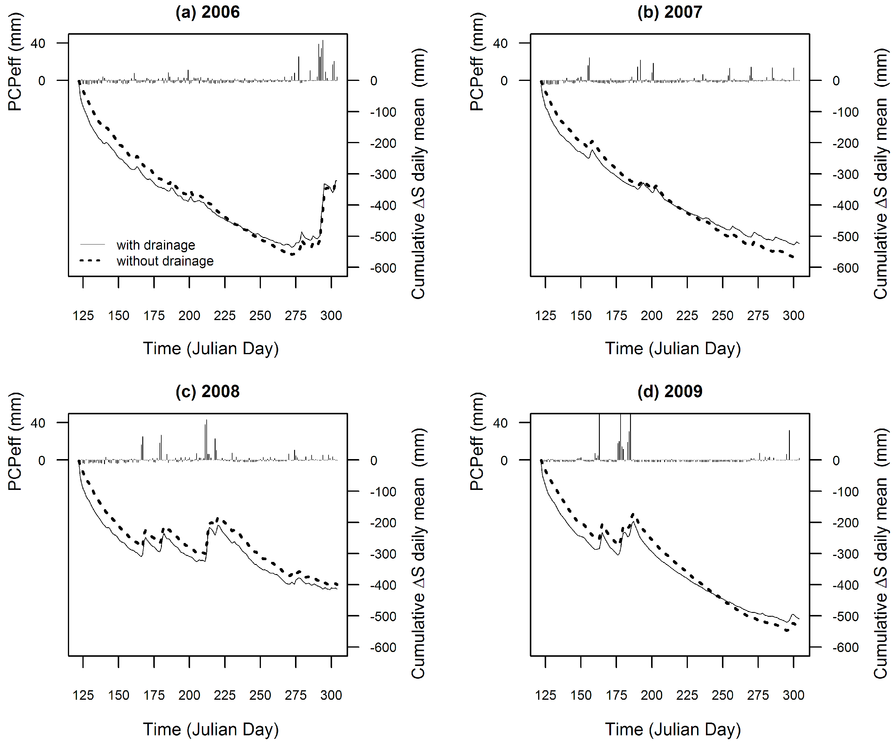
The values of total effective precipitation for the months of May to October are 343, 212, 337 and 382 mm for years 2006, 2007, 2008 and 2009, respectively. For 2006, precipitation was abundant near the end of the simulation period; that is, around mid-autumn (fall). Year 2007 was characterized by low precipitation and the lack of precipitation was seen over a large portion of the spring and summer. The wettest summer was in 2008, with high peaks of precipitation in spring, whereas year 2009 presents a lack of precipitation in summer.

Regional values of mean and median effective precipitation, as well as percentiles 25% and 75%, for the past forty years (1971 to 2010) for the period from 1 May to 31 October are 242, 220, 146, 329 mm, respectively. These regional values were established from the meteorological data in the database for the HYDROTEL model [56,57,58] applied to the Beaurivage watershed [59]. In this last application, precipitation and temperature were weighted means of the three stations nearest to the study site and the potential evapotranspiration was calculated with the equation developed at Hydro-Québec [57]. It can be observed that only the percentile 25% is lower than all effective precipitation values for all the years under study. Among the other three statistical measures of effective precipitation (mean, median and percentile 75%), only year 2007 has the lowest value. This confirms once again that not only year 2007 was the driest among the years being studied, but also it was regionally among the driest years over the past forty years.

At the beginning or first time step of each simulation, the initial soil water conditions are given by a water table set at 20 cm under the soil surface. This choice was based on the fact that the beginning of the simulations coincides with the spring season, which corresponds with the thawing period of the soil. It is known that, when the thaw ends, the water accumulated in the depressions infiltrates and reaches the water table to bring it closer to the soil surface in the Saint Lawrence lowlands [60]. The water table is generally near the surface early in spring, drops significantly during the summer months, and then rises again in the fall [61]. Furthermore, from a modelling point of view, under these spring conditions drainage systems fulfill their role when the initial water table is so high.

Subsurface drainage systems, located at 1.20 m from the soil surface (at the interface of the 7th and 8th layers), are represented by nodes to which was assigned a zero head pressure (i.e., atmospheric pressure), known as Dirichlet condition.

2.4.3. Variables Analyzed

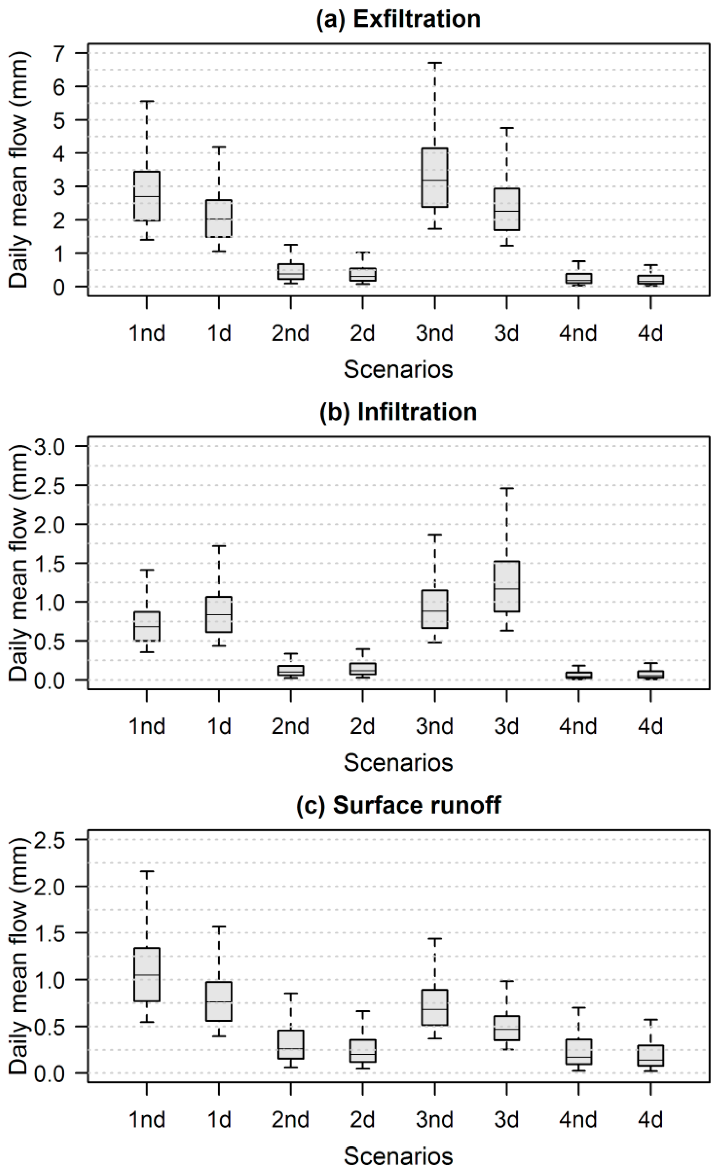
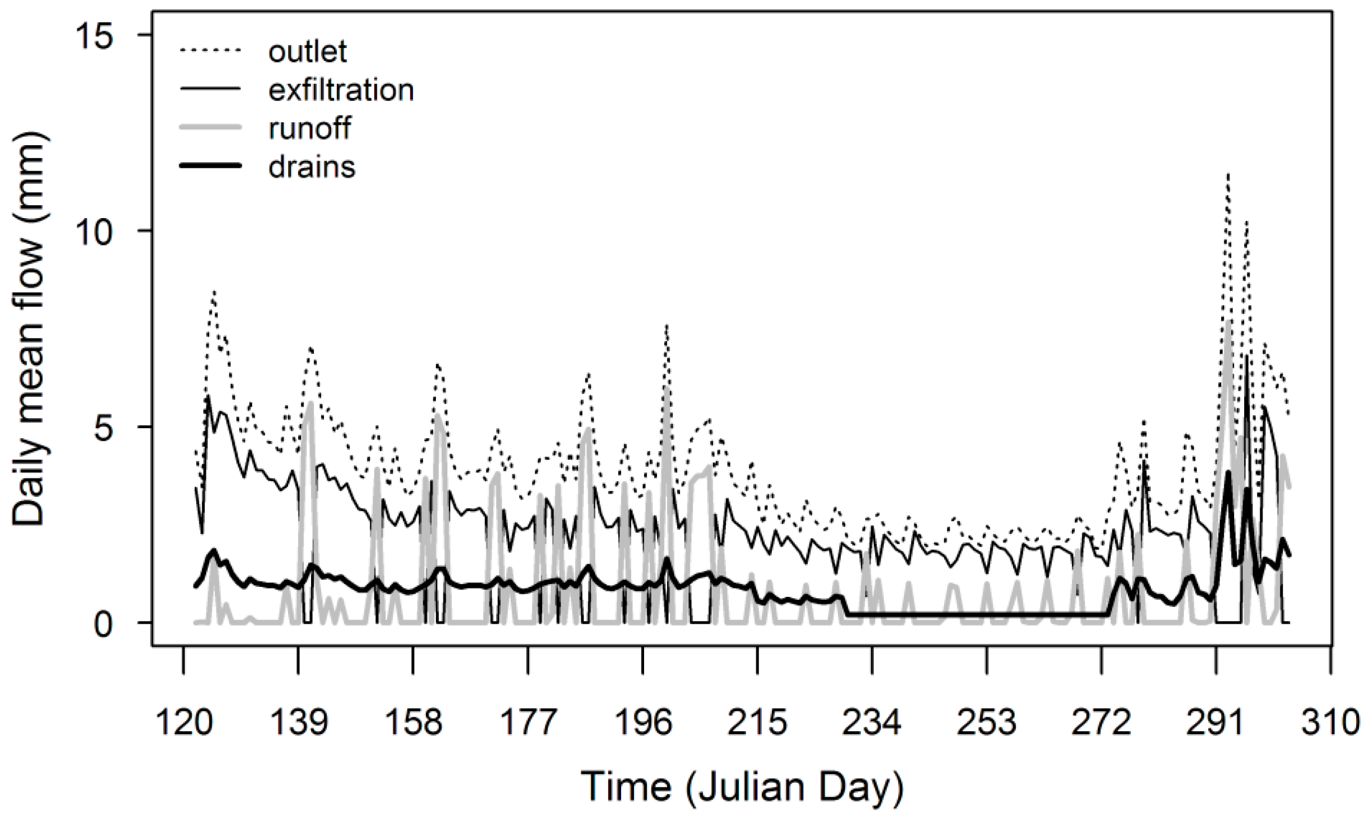
Figure 4 illustrates the different variables analysed. These are subsurface drain flow and micro-watershed outlet flow, storage variation, surface runoff, infiltration and exfiltration.

2.4.4. Evaluation of Model Performance

To evaluate the performance of the model, three criteria introduced in

Table 5. Evaluation of model performance.

Criteria	Statistical Approach	Best Value	Goal and Interpretation
Error in peak flow rate	$EP={\left[\frac{\max \left(O\right)-\max \left(P\right)}{\max \left(O\right)}\right]}_{i=1}^n$	0	- Minimize the criteria value. - Low (absolute) value: better performance, i.e., more precise simulation. - Zero (0) indicates that there is no difference between predicted and observed values.
Error in flow volume	$EV=\frac{{\displaystyle \sum _{i=1}^n{O}_i}-{\displaystyle \sum _{i=1}^n{P}_i}}{{\displaystyle \sum _{i=1}^n{O}_i}}$
Nash coefficient	$NSE=1-\frac{{\displaystyle \sum _{i=1}^n{\left(P_i-O_i\right)}^2}}{{\displaystyle \sum _{i=1}^n{\left(O_i-\overline{O}\right)}^2}}$	1	- Maximize the criteria value. - One (1) means that the model is perfect: simulated values are in perfect agreement with observed ones.

Note: n is the number of days during the simulation period. $O_i$ and $P_i$ are observed (measured) and predicted (simulated) discharges on Julian day i, respectively. $\overline{O}$ is the arithmetic mean of observed flows, and max and min are the maximum and minimum flow rates for the entire simulation period, respectively.

were used: the error in flow rate peaks (EP), error in flow volumes (EV), and Nash–Sutcliffe Evaluation criterion (NSE).

To account for the errors associated with observed flows from the measurement of water heights up to the establishment of the rating curve, a modified Nash criteria (NSE_m) was used [62], allowing ±20% error on the observed values as mentioned above. The formula reads as follows:

$$NS{E}_m=1-J$$

(3)

where NSE_m is the modified Nash criterion and J is defined as follows:

$$\{\begin{array}{c}\text{if }{P}_i < O_{i30}\text{ then }{J}_{i30}=\frac{{\displaystyle \sum _{i=1}^{N_{i30}}{\left(O_{i30}-P_i\right)}^2}}{{\displaystyle \sum _{i=1}^{N_{i30}}{\left(O_i-\overline{O}\right)}^2}}\\ \text{if }{P}_i > O_{i70}\text{ then }{J}_{i70}=\frac{{\displaystyle \sum _{i=1}^{N_{i70}}{\left(O_{i70}-P_i\right)}^2}}{{\displaystyle \sum _{i=1}^{N_{i70}}{\left(O_i-\overline{O}\right)}^2}}\end{array}$$

(4)

where P_i and O_i represent the simulated and observed flows on day J, respectively, and $\overline{O}$ is the arithmetic mean of observed flows during the simulation period. As mentioned above, if a simulated flow is included in the N_i30–70 values (for those included between O_i30 and O_i70), it is deemed sufficient and the value of the numerator J_i30–70 is zero by definition. Thus, NSE_m is merely the sum of J_i30 and J_i70.

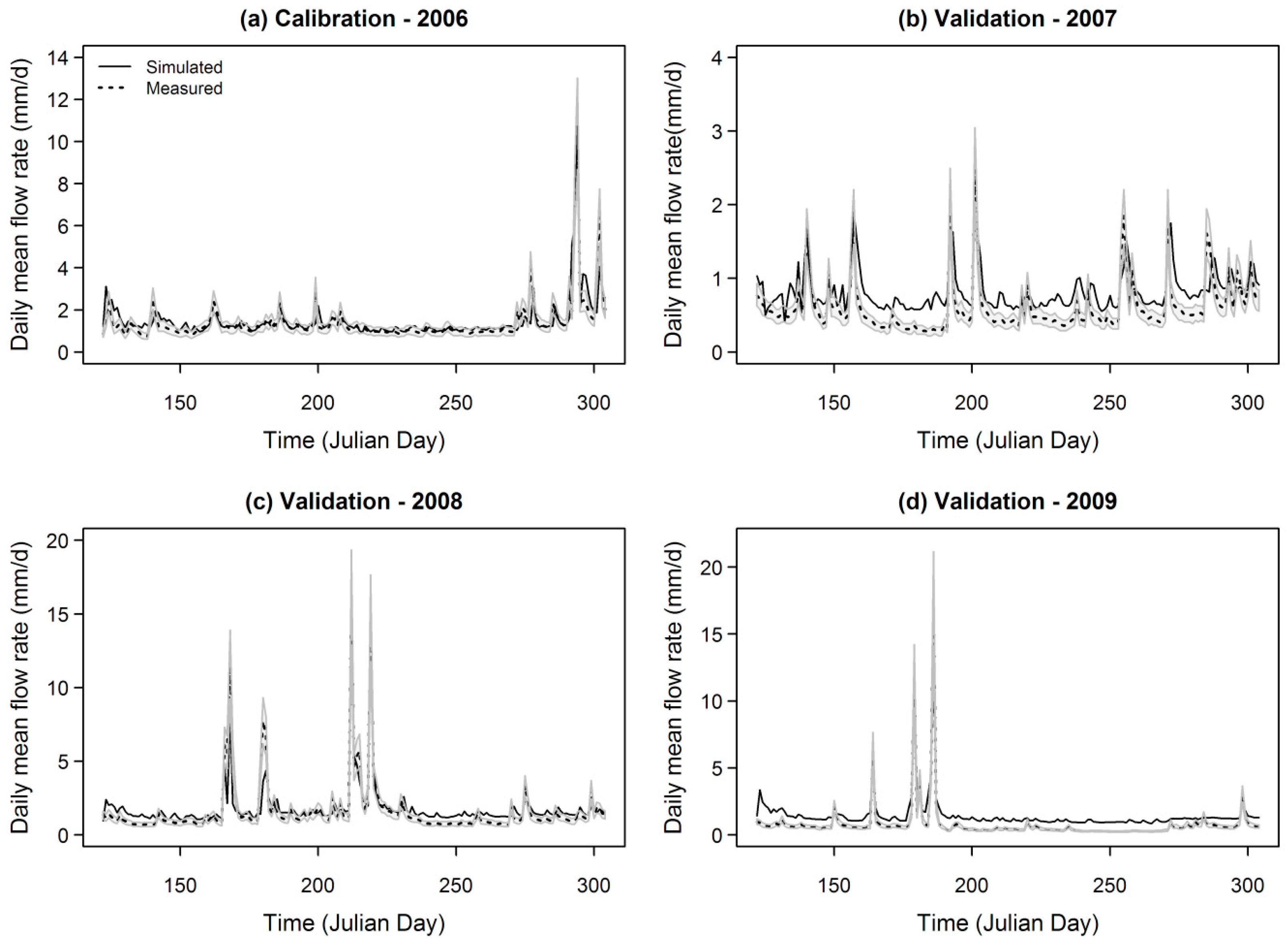
Flow measurement from year 2006 was used for the calibration process, whereas years 2007, 2008, and 2009 for the validation process with respect to the performance of the model and the storage variation behaviour according to different effective precipitation shapes.

3. Results

3.1. Simulation of the Flow at the Micro-Watershed Outlet and Analysis of the Effect of Subsurface Drainage on the Storage Variation

3.1.1. Calibration and Validation of the Model: Micro-Watershed Outlet Flow

Table 6. Model performance statistics.

Process	Year	EP	EV	NSE	NSEm
Calibration	2006	0.16	−0.04	0.71	0.89
Validation	2007	0.26	−0.33	0.17	0.69
	2008	0.36	−0.05	0.72	0.91
	2009	0.42	−0.74	0.67	0.81

introduces the values of the model performance statistics while Figure 5 presents measured and simulated flows, along with the uncertainty zone of ±20% on the observed values (in grey) depicted by the confidence interval of 30%–70% for the calibration year (2006) and the validation periods: (2007, 2008, and 2009). Since year 2006 has the smallest values of EP (0.16) and EV (−0.04), the resulting hydrographs demonstrate a good visual agreement between measured and simulated flows (Figure 5), corresponding to a good performance in terms of NSE (0.71). Over a large part of the hydrograph of years 2007 and 2009, measured flows are larger than those simulated, implying EP values (0.26 and 0.41, respectively) and EV (−0.33 and −0.74, respectively) values greater than 25%. From the fact that flow rates of year 2009 are greater than those of year 2007, the model performance was good (NSE = 0.67) for year 2009 and not acceptable for year 2007 (NSE = 0.17). Given that year 2008 has a lower gap between measured and simulated hydrographs for low flow rates compared to those of years 2007 and 2009, it has the smallest EV value (−0.05). Therefore, the model performance was good (NSE = 0.72).

Looking at the uncertainty zone (in grey) of ±20% with the 30%–70% confidence interval, years 2006 and 2008 are those where the simulated hydrographs are more or less within the uncertainty band. For low observed flow rates, the simulated hydrograph is generally not within the uncertainty zone especially for years 2007 and 2009. Thereby, the model performance increased from 0.71, 0.17, 0.72, and 0.67 in terms of NSE to 0.89, 0.69, 091, and 0.81 in terms of NSE_m for years 2006, 2007, 2008 and 2009, respectively. In this work, the model was calibrated according to the measured flow rates at the outlet. The distributed impact of subsurface drainage over catchment behaviour will be addressed in another paper.

3.1.2. Effect of Subsurface Drainage on Storage Variation

The daily mean storage variation (ΔS) cumulative curves with and without drainage systems in the porous media for each year and effective precipitation are illustrated in Figure 6 where two distinct behaviours are observed. The first relates to years 2006, 2007 and 2009, during which summer is characterized by low precipitation. These years, with low precipitation during summer period, present ΔS cumulative curves with and without drainage systems that intersect at a point on the simulation period. To the left of the point of intersection, the curve without drainage systems is above the one with drainage systems. To the right of the point of intersection, the situation reverses: the curve without drainage systems passes below that with drainage systems. The absence of flow from the subsurface drain networks in summer explained the inversion of the two curves (Figure 6a,b,d). The second behaviour concerned year 2008, which is the only one having registered the largest precipitation in the summer. The two curves with and without drainage systems remained almost parallel over the entire simulation period, with the second curve always above the first one (Figure 6c). According to time interval during which the curve with drainage systems is below that without subsurface drainage, more water was drained from the porous medium during 2008 while year 2007 yielded less drained water.

Considering a given ΔS variation (Y-axis) in the time intervals where the curve with drainage systems is below that with drainage systems, it can be seen that the time corresponding to the first curve is lower than the one for the second curve. This illustrates that drainage networks evacuate precipitation faster towards the outlet. Likewise, considering any time (X axis), it was observed that the ΔS curve with subsurface drainage systems is below that without subsurface drainage systems as said earlier (Figure 6c).

3.2. Impact of Subsurface Drainage and Soil Hydraulic Conductivity on Micro-Watershed Outlet Flow

Figure 7 presents the simulated cumulative outlet flow with and without subsurface drainage systems. It is noted that: (1) the flow in presence of subsurface drain systems is larger than in the situation without subsurface drainage for the four scenarios; (2) the lower the saturated hydraulic conductivities, the lower the flows (with and without subsurface drains); and (3) the gap or the difference between the hydrographs with and without subsurface drainage increases when saturated hydraulic conductivities are higher. Considering the cumulative flow values at the end of the simulations, for Sc. 1 to Sc. 4 those with subsurface drainage increase by 12.5%, 4.5%, 22.0% and 3.0%, respectively. Compared to those of Sc. 1, for Sc. 2 and Sc. 4 the flows decrease 60.0% and 75.0%, respectively, and increase to more than 10.0% for Sc. 3. The decreases or increase in flows with subsurface drainage were higher than those of flows without drainage.

Figure 8 presents the flow characteristics for Scenarios 1 to 4; namely: (a) daily mean flow expressed in form of box plot of logarithmic values; (b) maximum flow; and (c) minimum flow. For all of these scenarios, it was observed generally that the maximum flow without subsurface drainage is larger than that with subsurface drainage. Meanwhile, the reverse was observed for the minimum flow: the minimum flow without subsurface drainage is lower than that with drainage. As for cumulative flows at the end of each simulation, it was found that differences between extreme flows (maximum and minimum with and without drainage) are larger when the soil is more conductive (higher saturated hydraulic conductivity).

3.3. Impact of Subsurface Drainage and Soil Saturated Hydraulic Conductivity on Surface Runoff, Surface Water and Groundwater Coupling

Figure 9 presents the different flow values of exfiltration, infiltration and surface runoff for simulations with and without subsurface drainage systems for Sc. 1 to Sc. 4 in the form of box plots. From these results, it appears that generally exfiltration and surface runoff flows for simulations without subsurface drainage are higher than those with subsurface drainage. This situation is reversed when considering the infiltration process is concerned: flows are higher when simulations are with subsurface drain systems. Having the largest saturated hydraulic conductivity values, Sc. 3 presented highest variations in total exfiltration, infiltration and surface runoff between simulations with and without subsurface drainage systems. Since Sc. 4 had the smallest hydraulic conductivity values in the entire soil profile, it also had the smallest variations of exfiltration, infiltration and surface flows. It was also observed that scenarios having isotropic layers in the first group of layers (surface layers), namely Sc. 3 and Sc. 4, yielded infiltration and surface runoff flow variations that are almost equal.

3.4. Impact of Subsurface Drainage and Soil Saturated Hydraulic Conductivity on the Outlet Flow Hydrograph

The hydrograph of the daily mean flow at the micro-watershed outlet and its different components for Sc. 1 are presented in Figure 10. It was observed that: (1) exfiltration is the most dominant flow; (2) peaks of the hydrograph are largely dominated by surface runoff; and (3) subsurface drain flow variations are low and tend to zero during the period where there precipitation was very low.

The cumulative flow at the outlet of the micro-watershed and its various components, and its relation with them for Sc. 1 to Sc. 4 are illustrated in Figure 11. For Sc. 1, these curves show that exfiltration, subsurface drain flow and surface runoff represent 56%, 23% and 21% of the cumulative flow at the outlet of the micro-watershed, respectively. Given that the micro-watershed is artificially drained over 30% of its area, the contribution of the subsurface drain networks to the micro-watershed outlet is significant.

Considering the values of exfiltration (E) and subsurface drain flow (D) over outlet flow (O) (i.e., E/O and D/O) in decreasing order, the scenarios can be classified as follows: Sc. 3, Sc. 1, Sc. 2 and Sc. 4. On the other hand, from the point of view of the decrease in the ratio of the surface runoff (R) over outlet flow (O) (i.e., R/O), they can be classified in the order Sc. 4, Sc. 2, Sc. 1 and Sc. 3. Thus, it was observed that when the soil is more conductive, the exfiltration and subsurface drain flows are higher while the surface runoff flow is lower.

When the last two contributing flows are further analysed (subsurface drain flow and surface runoff), it should be noted that for Sc. 1, subsurface drain flow is slightly larger than surface runoff. For Sc. 3, where the soil is more conductive than for Sc. 1, subsurface drain flow is significantly larger than surface runoff. For Sc. 2 and Sc. 4, where soils are less conductive than for Sc. 1, the surface runoff is larger than the subsurface drain flow.

4. Discussion

4.1. Simulation of the Flow at the Micro-Watershed Outlet and Analysis of the Effect of Subsurface Drainage on the Storage Variation

Given the simulated flow results obtained at the micro-watershed outlet, the performance of CATHY was deemed satisfactory. It was better when the effective precipitation was larger; corresponding to large observed and simulated flows. Subsurface drainage is a needful agricultural practice during periods with high water tables under the effect of high precipitation or irrigation [1,2]. This study demonstrated that CATHY can reliably predict subsurface drainage flow during wet periods; that is the time when it is imperative to know whether a drainage system can meet design criteria.

When considering the dynamics of the cumulative storage variation, results showed that the behaviour depended not only on the amount of precipitation but also on the associated distribution throughout the year. For a year with more summer precipitation, the simulation curve with subsurface drains remained in general below the curve without subsurface drains, indicating that there was subsurface-drain flow throughout the simulation period. In the presence of low summer precipitation, the first curve was below the second one, illustrating the absence of flow through the subsurface drainage networks. When the first curve was below the second one, the implication is that not only did subsurface agricultural drains evacuate precipitation very fast, but they increased the flow at the outlet of the micro-watershed. This means that subsurface drains increase the amount of water flowing from the soil toward the watershed outlet by diminishing the water content of the soil [63]. Konyha et al. found that the total flow exiting from a drained field could increase by 10% [64]. Since the drains route a portion of the subsurface flow faster toward surface waters (outlet), this results in a decrease of storage in the porous media-less water being actually stored in the soil profile-and an increase in the micro-watershed outlet flow. The implementation of a subsurface drainage network generally entails a reduction of the response time of agricultural plots [65,66].

4.2. Impact of Subsurface Drainage and Soil Hydraulic Conductivity on the Micro-Watershed Outlet Flow

Tile drains can substantially alter the total water yield from a field or small watershed as well as modify the timing and shape of the hydrograph [8]. Tile drainage increases the proportion of annual precipitation that is discharged to surface waters via subsurface flow relative to the amount that is stored, evaporated or transpired [9,10,11]. Total water yield from a field tends to increase with the installation of subsurface drainage while surface runoff and sediment yield are often significantly decreased [2,16,17].

By increasing the drainage capacity of the soils, it was observed at the micro-watershed outlet that: (a) agricultural subsurface drains increased the cumulative mean daily and base (minimum) flows, and decreased peak flows (maximum); (b) the smaller were the saturated hydraulic conductivities, the smaller were the flows (with or without subsurface drainage); (c) the gap between the cumulative flow curve with drainage and that without drainage increased when saturated hydraulic conductivities were higher; and (d) the differences between extreme flows (maximum and minimum with and without drainage) were higher when the soil was more conductive (greater values of saturated hydraulic conductivity).

4.3. Impact of Subsurface Drainage and Soil Saturated Hydraulic Conductivity on Surface Runoff, Surface Water and Groundwater Coupling

Several studies have dealt with the impact of subsurface agricultural drainage on the hydrology of fields and watersheds. The implementation of a network of drains generally entails a reduction in surface runoff by increasing infiltration of precipitation [67,68,69,70]. The changes associated with subsurface agricultural drainage according to soil properties have an impact on the hydrologic budget by altering subsurface water flow, in particular, flows to the surface (watershed outlet) by exfiltration. That being said, soil properties, in particular saturated hydraulic conductivity, may affect the extent to which subsurface drainage can influence subsurface flow [67].

When considering surface and subsurface waters, drains reduced exfiltration and surface runoff, and increased infiltration. The more conductive were the soils, the more exfiltration and subsurface drain flows were higher, whereas surface runoff was lower, and for isotropic surface layers, the variations in surface runoff and infiltration were almost equal. Most soils are heterogeneous and anisotropic; that is, hydraulic properties vary in space and are higher in a given direction [71]. When considering isotropy and anisotropy of the soil layer groups, it is evident that these properties play an important role on exfiltration, surface runoff and infiltration of water, and consequently on flows (maximum, minimum and total) at the micro-watershed outlet.

4.4. Behavior of the Outlet Hydrograph Components

Groundwater discharge to streams is commonly expressed as base flow, which is streamflow that occurs during dry times of the year [72]. Groundwater contribution is very low during the flood periods but can be very important at the annual scale and surface runoff is the most significant component in observed flows during floods [73]. When analysing the outlet hydrograph, it was noticed that: (a) exfiltration was the dominant process; (b) peaks were largely dominated by surface runoff; and (c) variations in subsurface drain flow were low.

5. Conclusions

The corner stone of this study was the application of CATHY, a 3D hydrological model, to assess the influence of artificial subsurface drainage on flows at the watershed level. Flows simulated by CATHY at the outlet of the study watershed corroborated well with observed data mostly during wet years. For these years, subsurface water flows easily towards the micro-watershed outlet via drains, allowing the model to properly simulate the flows at the outlet of micro-watershed. Furthermore, simulations were consistent with the traditional approaches of subsurface drainage effects on surface and subsurface components such as base and peak flows, surface runoff, infiltration, and exfiltration.

The development of scenarios aims to support management practices such as the effect of tillage on infiltration or percolation of rain in soil layers. Next to that, when measuring the saturated hydraulic conductivities in situ or in laboratory, their values can fluctuate within a certain range of order 10. The aim of this study was conducted in this context.

These types of studies are needed to build our capacities to manage water resources in agricultural watersheds, where water flow dynamics are often manipulated to increase productivity. A good control of the impact of these manipulations will result in a better understanding of the flows and improved design of management actions to reduce the risks of degrading the quality of surface waters.

References

1. Eggelsmann, R. Dränanleitung für den Landbau, Ingenieurbau und Landschaftsbau, 2nd ed.; Verlag Paul Parey: Hamburg, Germany, 1981. [Google Scholar]
2. Skaggs, R.W.; Brevé, M.A.; Gilliam, J.W. Hydrologic and water quality impacts of agricultural drainage. Crit. Rev. Environ. Sci. Technol. 1994, 24, 1–32. [Google Scholar] [CrossRef]
3. Eidman, V. Minnesota farmland drainage: Profitability and concerns. Minn. Agric. Econ. 1997. No 688. Department of Applied Economics, University of Minnesota, St. Paul, MN, USA, 1997. Available online: http://ageconsearch.umn.edu/bitstream/13165/1/mae688a.pdf (accessed on 2 June 2015). [Google Scholar]
4. Fausey, N.R. Drainage: Inadequacy and crop response. In Encyclopedia of Water Science; Stewart, B.A., Howell, T., Eds.; Taylor and Francis: Oxford, UK, 2003; pp. 132–134. [Google Scholar]
5. Fausey, N.R. Drainage management for humid regions. Int. Agric. Eng. J. 2005, 14, 209–214. [Google Scholar]
6. Basin Technical and Scientific Advisory Committee (BTSAC). Water Management Options for Subsurface Drainage: Briefing Paper 2. 2012. Available online: http://www.rrbdin.org/archives/4520 (accessed on 28 June 2014).
7. St-Hilaire, A.; Duchesne, A.S.; Rousseau, A.N. Floods and water quality in Canada—A review of the interactions with urbanization, agriculture and forestry. Can. Water Resour. J. 2015, 41, 273–287. [Google Scholar] [CrossRef]
8. Schilling, K.E.; Helmers, M. Effects of subsurface drainage tiles on streamflow in Iowa agricultural watersheds: Exploratory hydrograph analysis. Hydrol. Process. 2008, 22, 4497–4506. [Google Scholar] [CrossRef]
9. Serrano, S.E.; Whiteley, H.R.; Irwin, R.W. Effects of agricultural drainage on streamflow in the Middle Thames River, Ontario, 1949–1980. Can. J. Civ. Eng. 1985, 12, 875–885. [Google Scholar] [CrossRef]
10. Magner, J.A.; Payne, G.A.; Steffen, L.J. Drainage effects on stream nitrate-n and hydrology in south-central Minnesota (USA). Environ. Monit. Assess. 2004, 91, 183–198. [Google Scholar] [CrossRef] [PubMed]
11. Tomer, M.D.; Meek, D.W.; Kramer, L.A. Agricultural practices influence flow regimes of headwater streams in Western Iowa. J. Environ. Qual. 2005, 34, 1547–1558. [Google Scholar] [CrossRef] [PubMed]
12. King, K.W.; Fausey, N.R.; Williams, M.R. Effect of subsurface drainage on streamflow in an agricultural headwater watershed. J. Hydrol. 2014, 519, 438–445. [Google Scholar] [CrossRef]
13. Macrae, M.L.; English, M.C.; Schiff, S.L.; Stone, M. Intra-annual variability in the contribution of tile drains to basin discharge and phosphorus export in a first-order agricultural catchment. Agric. Water Manag. 2007, 92, 171–182. [Google Scholar] [CrossRef]
14. Culley, J.L.B.; Bolton, E.F. Suspended solids and phosphorus loads from a clay soil: II. Watershed study. J. Environ. Qual. 1983, 12, 498–503. [Google Scholar] [CrossRef]
15. Xue, Y.; David, M.B.; Gentry, L.E.; Kovacic, D.A. Kinetics and modeling of dissolved phosphorus export from a tile-drained agricultural watershed. J. Environ. Qual. 1998, 27, 917–922. [Google Scholar] [CrossRef]
16. Robinson, M.; Rycroft, D.W. The impact of drainage on stream flows. Agron. Monogr. 1999, 38, 767–800. [Google Scholar]
17. Dolezal, F.; Kulhavy, Z.; Soukup, M.; Kodesova, R. Hydrology of tile drainage runoff. Phys. Chem. Earth B Hydrol. Ocean Atmos. 2001, 26, 623–627. [Google Scholar] [CrossRef]
18. Robinson, M. Impact of Improved Land Drainage on River Flows; Institute of Hydrology Center for Ecology and Hydrology: Edinburgh, UK, 1990. [Google Scholar]
19. Bengtson, R.L.; Carter, C.E.; Fouss, J.L.; Southwick, L.M.; Willis, G.H. Agricutural drainage and water quality in the Mississippi delta. J. Irrig. Drain. Eng. 1995, 121, 292–295. [Google Scholar] [CrossRef]
20. Zucker, L.A.; Brown, L.C.E. (Eds.) Agricultural Drainage: Water Quality Impacts and Subsurface Drainage Studies in the Midwest; The Ohio State University: Columbus, OH, USA, 1998.
21. Kleinman, P.J.A.; Smith, D.R.; Bolster, C.H.; Easton, Z.M. Phosphorus Fate, Management, and Modeling in Artificially Drained Systems. J. Environ. Qual. 2015, 44, 460–466. [Google Scholar] [CrossRef] [PubMed]
22. Wiskow, E.; van der Ploeg, R.R. Calculation of drain spacings for optimal rainstorm flood control. J. Hydrol. 2003, 272, 163–174. [Google Scholar] [CrossRef]
23. King, K.W.; Williams, M.R.; Faussey, N.R. Contributions of systematic tile drainage to watershed-scale phosphorus transport. J. Environ. Qual. 2015, 44, 486–494. [Google Scholar] [CrossRef] [PubMed]
24. Smith, D.R.; King, K.W.; Johnson, L.; Francesconi, W.; Richards, P.; Baker, D.; Sharpley, A.N. Surface runoff and tile drainage transport of phosphorus in the midwestern United States. J. Environ. Qual. 2015, 44, 495–502. [Google Scholar] [CrossRef] [PubMed]
25. Schottler, S.P.; Ulrich, J.; Belmont, P.; Moore, R.; Lauer, W.J.; Engstrom, D.R.; Almendinger, J.E. Twentieth century agricultural drainage creates more erosive rivers. Hydrol. Process. 2014, 28, 1951–1961. [Google Scholar] [CrossRef]
26. Dunn, S.M.; Mackay, R. Modelling the hydrological impact of open ditch drainage. J. Hydrol. 1996, 179, 37–66. [Google Scholar] [CrossRef]
27. Holden, J.; Chapman, P.J.; Labadz, J.C. Artificial drainage of peatlands: Hydrological andhydrochemical process and wetland restoration. Prog. Phys. Geogr. 2004, 28, 95–123. [Google Scholar] [CrossRef]
28. Vidon, P.; Cuadra, P.E. Phosphorus dynamics in tile-drain flow during storms in the US Midwest. Agric. Water Manag. 2011, 98, 532–540. [Google Scholar] [CrossRef]
29. Kung, K.J.S.; Kladivko, E.J.; Gish, T.J.; Steenhuis, T.S.; Bubenzer, G.; Helling, C.S. Quantifying preferential flow by breakthrough of sequentially applied tracers: Silt loam soil. Soil Sci. Soc. Am. J. 2000, 64, 1296–1304. [Google Scholar] [CrossRef]
30. Bixio, A.C.; Orlandini, S.; Paniconi, C.; Putti, M. Modeling groundwater-surface water interactions including effects of morphogenetic depressions in the Chernobyl exclusion zone. Environ. Geol. 2002, 42, 162–177. [Google Scholar] [CrossRef]
31. Orlandini, S. On the spatial variation of resistance to flow in upland channel networks. Water Resour. Res. 2002, 38, 1197. [Google Scholar] [CrossRef]
32. Paniconi, C.; Troch, P.A.; van Loon, E.E.; Hilberts, A.G.J. Hillslope-storage Boussinesq model for subsurface flow and variable source areas along complex hillslopes: 2. Intercomparison with a three-dimensional Richards equation model. Water Resour. Res. 2003, 39, 1317. [Google Scholar] [CrossRef]
33. D'Haese, C.M.F.; Putti, M.; Paniconi, C.; Verhoest, N.E.C. Assessment of adaptive and heuristic time stepping for variably saturated flow. Int. J. Numer. Methods Fluids 2007, 53, 1173–1193. [Google Scholar] [CrossRef]
34. Gauthier, M.J.; Camporese, M.; Rivard, C.; Paniconi, C.; Larocque, M. A modeling study of heterogeneity and surface water-groundwater interactions in the Thomas Brook catchment, Annapolis Valley (Nova Scotia, Canada). Hydrol. Earth Syst. Sci. 2009, 13, 1583–1596. [Google Scholar] [CrossRef]
35. Sulis, M.; Meyerhoff, S.B.; Paniconi, C.; Maxwell, R.M.; Putti, M.; Kollet, S.J. A comparison of two physics-based numerical models for simulating surface water-groundwater interactions. Adv. Water Resour. 2010, 33, 456–467. [Google Scholar] [CrossRef]
36. Sulis, M.; Paniconi, C.; Camporese, M. Impact of grid resolution on the integrated and distributed response of a coupled surface–subsurface hydrological model for the des Anglais catchment, Quebec. Hydrol. Process. 2011, 25, 1853–1865. [Google Scholar] [CrossRef]
37. Sulis, M.; Paniconi, C.; Rivard, C.; Harvey, R.; Chaumont, D. Assessment of climate change impacts at the catchment scale with a detailed hydrological model of surface-subsurface interactions and comparison with a land surface model. Water Resour. Res. 2011, 47, W01513. [Google Scholar] [CrossRef]
38. Broda, S.; Paniconi, C.; Larocque, M. Numerical investigation of leakage in sloping aquifers. J. Hydrol. 2011, 409, 49–61. [Google Scholar] [CrossRef]
39. Zanello, F.; Teatini, P.; Putti, M.; Gambolati, G. Long term peatland subsidence: Experimental study and modeling scenarios in the Venice coastland. J. Geophys. Res. Earth Surf. 2011, 116, F04002. [Google Scholar] [CrossRef]
40. Dagès, C.; Paniconi, C.; Sulis, M. Analysis of coupling errors in a physically-based integrated surface water-groundwater model. Adv. Water Resour. 2012, 49, 86–96. [Google Scholar] [CrossRef]
41. Guay, C.; Nastev, M.; Paniconi, C.; Sulis, M. Comparison of two modeling approaches for groundwater–surface water interactions. Hydrol. Process. 2013, 27, 2258–2270. [Google Scholar] [CrossRef]
42. Passadore, G.; Monego, M.; Altissimo, L.; Sottani, A.; Putti, M.; Rinaldo, A. Alternative conceptual models and the robustness of groundwater management scenarios in the multi-aquifer system of the Central Veneto Basin, Italy. Hydrogeol. J. 2012, 20, 419–433. [Google Scholar] [CrossRef]
43. Niu, G.-Y.; Paniconi, C.; Troch, P.A.; Scott, R.L.; Durcik, M.; Zeng, X.; Huxman, T.; Goodrich, D.C. An integrated modelling framework of catchment-scale ecohydrological processes: 1. Model description and tests over an energy-limited watershed. Ecohydrology 2013, 7, 427–439. [Google Scholar] [CrossRef]
44. Lamontagne, L.; Martin, A.; Nolin, M.C. Étude Pédologique du Bassin Versant du Bras d'Henri (Québec); Laboratoires de Pédologie et D’agriculture de Précision, Centre de Recherche et de Développement sur les sols et les Grandes Cultures, Service National D’information sur les Terres et les eaux, Direction Générale de la Recherche, Agriculture et Agroalimentaire Canada: Sainte-Foy, QC, Canada, 2010. [Google Scholar]
45. Agriculture & Agri-Food Canada. Greencover Canada. Government of Canada. 2004a. Available online: http://www.agr.gc.ca/env/greencover-verdir/index_e.phtml (accessed on 20 May 2015).
46. Agriculture & Agri-Food Canada. Watershed Evaluation of BMPs (WEBs). Government of Canada. 2004b. Available online: http://www.agr.gc.ca/env/greencover-verdir/webs_abstract_e.phtml (accessed on 20 May 2015).
47. Agriculture & Agri-Food Canada. Watershed Evaluation of BMPs (WEBs). Government of Canada. 2004c. Available online: http://www.agr.gc.ca/AAFC-AAC/displa-afficher.do?id=1228497657135&lang=eng (accessed on 20 May 2015).
48. Muma, M.; Gumiere, S.J.; Rousseau, A.N. Analyses de sensibilité globales du modèle CATHY aux propriétés hydrodynamiques du sol d’un micro-bassin agricole drainé. Hydrol. Sci. J. 2014, 59, 1606–1623. [Google Scholar] [CrossRef]
49. Ratte-Fortin, C. Développement d’une Méthode D’évaluation de L’impact de Pratiques de Gestion Bénéfiques sur les Flux de Contaminants Agricoles: Cas du Micro-Bassin Versant D’intervention du Bras d’Henri, Québec, Canada; Mémoire de Maîtrise, Institut National de la Recherche Scientifique—Centre Eau Terre Environnement (INRS-ETE): Ville de Québec, QC, Canada, 2014. [Google Scholar]
50. Bouwer, H.; Rice, R.C. A slug test for determining hydraulic conductivity of unconfined aquifers with completely or partially penetrating wells. Water Resour. Res. 1976, 12, 424–428. [Google Scholar] [CrossRef]
51. Pandit, N.S.; Miner, R.F. Interpretation of slug test data. Ground Water 1986, 24, 743–749. [Google Scholar] [CrossRef]
52. Camporese, M.; Paniconi, C.; Putti, M.; Orlandini, S. Surface-subsurface flow modeling with path-based runoff routing, boundary condition-based coupling, and assimilation of multisource observation data. Water Resour. Res. 2010, 46, W02512. [Google Scholar] [CrossRef]
53. Paniconi, C.; Putti, M. A comparison of Picard and Newton iteration in the numerical solution of multidimensional variably saturated flow problems. Water Resour. Res. 1994, 30, 3357–3374. [Google Scholar] [CrossRef]
54. Ministère de l’Agriculture, des Pêcheries et de l’Alimentation du Québec (MAPAQ). Profil de la région Chaudière-Appalaches (région 12)-Climat [en ligne]. Ministère de l’Agriculture, Pêcheries et Alimentation du Québec: Canada, 2007. Available online: http://www.mapaq.gouv.qc.ca/Fr/Regions/chaudiereappalache/vraiprofil/ (accessed on 26 June 2015). [Google Scholar]
55. Allen, R.G.; Pereira, L.S.; Raes, D.; Smith, M. Crop Evapotranspiration: Guidelines for Computing Crop Water Requirements; Irrigation and Drainage, FAO: Roma, Italy, 1998. [Google Scholar]
56. Fortin, J.P.; Turcotte, R.; Massicotte, S.; Moussa, R.; Fitzback, J.; Villeneuve, J.P. A distributed watershed model compatible with remote sensing and GIS data. Part 1: Description of the model. J. Hydrol. Eng. 2001, 6, 91–99. [Google Scholar] [CrossRef]
57. Fortin, J.P.; Turcotte, R.; Massicotte, S.; Moussa, R.; Fitzback, J.; Villeneuve, J.P. A distributed watershed model compatible with remote sensing and GIS data. Part 2: Application to the Chaudière Watershed. J. Hydrol. Eng. 2001, 6, 100–108. [Google Scholar] [CrossRef]
58. Fortin, J.P.; Moussa, R.; Bocquillon, C.; Villeneuve, J.P. Hydrotel, un model hydrologique distribué pouvant bénéficier des données fournies par la télédétection et les systèmes d'information géographique. Rev. Sci. de l'Eau 1995, 8, 97–124. [Google Scholar] [CrossRef]
59. Rousseau, A.N.; Savary, S.; Hallema, D.W.; Gumiere, S.J.; Foulon, E. Modeling the effects of agricultural BMPs on sediments, nutrients and water quality of the Beaurivage River watershed (Quebec, Canada). Can. Water Resour. J. 2013, 38, 99–120. [Google Scholar] [CrossRef]
60. Lagacé, R. Infiltration et Drainage, Notes de Cours: Bilan Hydrique au Québec. Département des Sols et de Génie Agroalimentaire, Université Laval: Québec City, QC, Canada, 2012. Available online: http://www.grr.ulaval.ca/gaa_7003/Documents/Notes_cours_2012/CH_10_Bilan_QC.pdf (accessed on 12 January 2015).
61. Savoie, V. Le Drainage de Surface; Formation OAQ, MAPAQ: Centre du Québec, QC, Canada, 2009. [Google Scholar]
62. Bessière, H. Assimilation de Données Variationnelles Pour la Modélisation Hydrologique Distribuée des Crues à Cinétique Rapide. Thèse de Doctorat, Université de Toulouse, Institut National Polytechnique de Toulouse, Toulouse, France, 2008. [Google Scholar]
63. Larson, C.L.; Moore, I.D. Hydrologic impact of draining small depressional watersheds. J. Irrig. Drain. Div. 1980, 104, 345–363. [Google Scholar]
64. Konyha, K.D.; Skaggs, R.W.; Gilliam, J.W. Effects of drainage and water management practices on hydrology. J. Irrig. Drain. Eng. 1992, 118, 807–819. [Google Scholar] [CrossRef]
65. Bailey, A.D.; Bree, T. Effect of improved land drainage on river flood flows. In Flood Studies Report-Five Years on; Thomas Talford: London, UK, 1981; pp. 95–106. [Google Scholar]
66. Rycrott, D.W.; Massey, W. The Effect of Field Drainage on the River Flood Flows; Field Drainage Experimental Unit, MAFF: London, UK, 1975. [Google Scholar]
67. Hill, A.R. The environmental impacts of agricultural land drainage. J. Environ. Manag. 1976, 4, 251–274. [Google Scholar]
68. Irwin, R.W.; Whitely, H.R. Effects of land drainage on stream flow. Can. Water Resour. J. 1983, 8, 88–103. [Google Scholar] [CrossRef]
69. Thomas, D.L.; Perry, C.D.; Evans, R.O.; Izuno, F.T.; Stone, K.C.; Gilliam, J.W. Agricultural drainage effects on water quality in Southeastern U.S. J. Irrig. Drain. Eng. 1995, 121, 277–282. [Google Scholar] [CrossRef]
70. Watelet, A.; Johnson, P.G. Hydrology and water quality of the Raisin River: Overview of impacts of recent land and channel changes in Eastern Ontario. Can. J. Water Qual. Res. 1999, 34, 361–390. [Google Scholar]
71. Kasenow, M. Determination of Hydraulic Conductivity from Grain Size Analysis; Water Resources Publications, L.L.C.: Highlands, CO, USA, 2010. [Google Scholar]
72. Winkler, R.D.; Moore, R.D.; Redding, T.E.; Spittlehouse, D.L.; Carlyle-Moses, D.E.; Smerdon, B.D. Hydrologic Processes and Watershed Response. In Compendium of Forest Hydrology and Geomorphology in British Columbia; Pike, R.G., Redding, T.E., Moore, R.D., Winkler, R.D., Bladon, K.D., Eds.; B.C. Min. For. Range, For. Sci. Prog., Victoria, B.C. and FORREX Forum for Research and Extension in Natural Resources, Kamloops, B.C. Land Manag. Handb; Government Publications Services: Victoria, BC, Canada, 2000. [Google Scholar]
73. Bennis, S. Hydraulique et Hydrologie, 2e Édition Revue et Augmentée; Presses de l’Université du Québec: Ville de Québec, QC, Canada, 2009. [Google Scholar]
Figure 1. Location of the Bras d’Henri micro-watershed.
Water 08 00326 g001
Figure 2. (a) Spatial distribution of different soil families; and (b) locations of subsurface drain systems and piezometers in the micro-watershed (blue lines are stream network, other colours are subsurface drainage systems, the star indicates the micro-watershed outlet, and dots are piezometers) (adapted from Muma et al. [48]).
Water 08 00326 g002
Figure 3. Representation of saturated hydraulic conductivity values representation in the different layers of the porous medium in the form of diagrams.
Water 08 00326 g003
Figure 4. Illustration of the analysed variables: outlet flow, drained flow, runoff, infiltration, exfiltration and storage variation (ΔS with St+1 the storage at current time step and St the storage at previous time step).
Water 08 00326 g004
Figure 5. Measured and simulated flows along with the uncertainty zone of ±20% on the observed values (in grey) depicted by the confidence interval of 30%–70% for the (a) calibration year (2006) and the validation periods: (b) 2007; (c) 2008; and (d) 2009.
Water 08 00326 g005
Figure 6. Effect of subsurface drain systems on the cumulative storage variation in the micro-watershed for: (a) the calibration period (2006) and the validation periods: (b) 2007; (c) 2008; and (d) 2009.
Water 08 00326 g006
Figure 7. Cumulative daily mean flow at the micro-watershed outlet for Scenarios 1 to 4 with labels “d” and “nd” representing simulations with and without drainage systems, respectively.
Water 08 00326 g007
Figure 8. Micro-watershed outlet daily mean flows: (a) log-transformed daily mean flow; (b) their maximum values; and (c) their minimum values (“d” and “nd” expressing simulation with and without subsurface drainage, respectively) for Scenarios 1 to 4.
Water 08 00326 g008
Figure 9. Impact of subsurface drain networks and soils on exfiltration (a); infiltration (b) and surface (c) flows in form of box plots (outlier omitted) with “d” and “nd” expressing simulation with and without subsurface drainage, respectively for Scenarios 1 to 4.
Water 08 00326 g009
Figure 10. Hydrograph of daily mean flow at micro-watershed outlet and its different components (exfiltration, runoff, and drains) for Scenario 1.
Water 08 00326 g010
Figure 11. Curves of cumulative flow at the micro-watershed outlet (O) and its different components (exfiltration: E, drains: D and runoff: R) of: (a) Scenario 1; (b) Scenario 2; (c) Scenario 3; (d) Scenario 4; and (e) ratios of E, D, R over O.
Water 08 00326 g011