Development of Dynamic Ground Water Data Assimilation for Quantifying Soil Hydraulic Properties from Remotely Sensed Soil Moisture

Abstract

Several inversion modeling-based approaches have been developed/used to extract soil hydraulic properties (α, n, θ_res, θ_sat, K_sat) from remotely sensed (RS) soil moisture footprints. Hydrological models with shallow ground water (SGW) table depths in soils simulate daily root zone soil moisture dynamics based on the extracted soil parameters. The presence of SGW table depths in soils significantly influences model performances; however, SGW table depths are usually unknown in the field, thus, unknown SGW table depths might cause uncertainties in the model outputs. In order to overcome these drawbacks, we developed a dynamic ground water (DGW) data assimilation approach that can consider SGW table depths across time for quantifying effective soil hydraulic properties in the unsaturated zone. In order to verify the DGW data assimilation scheme, numerical experiments comprising synthetic and field validation experiments were conducted. For the numerical studies, the Little Washita (LW) watershed in Oklahoma and Olney (OLN)/Bondville (BOND) sites in Illinois were selected as different hydroclimatic regions. For the synthetic conditions, we tested the DGW scheme using various soil textures and vegetation covers with fixed and dynamically changing SGW table depths across time in homogeneous and heterogeneous (layered) soil columns. The DGW-based soil parameters matched the observations under various synthetic conditions better than those that only consider fixed ground water (FGW) table depths in time. For the field validations, our proposed data assimilation scheme performed well in predicting the soil hydraulic properties and SGW table depths at the point, airborne sensing, and satellite scales, even though uncertainties exist. These findings support the robustness of our proposed DGW approach in application to regional fields. Thus, the DGW scheme could improve the availability and applicability of pixel-scale soil moisture footprints based on satellite platforms.

1. Introduction

Root zone soil moisture is the pivotal component of hydrology, meteorology, and agriculture across the world. Direct and indirect schemes can be used for estimating root zone soil moisture in the spatial and temporal domains. In general, the direct approach has relatively high accuracy at the point scale, with some disadvantages (e.g., high cost, time-consuming, limited availability at spatial–temporal scales). In order to overcome these drawbacks, remotely sensed (RS) soil moisture footprints as an indirect method have been suggested as an alternative [1,2,3]. The land surface soil moisture estimates were derived based on thermal infrared remote sensing [4]. Furthermore, Njoku and Entekkabi [5] developed direct active/passive microwave remote sensing schemes for estimating land surface soil moisture values.

A few inversion models linked with hydrological models have been developed/used for deriving the soil hydraulic properties (α, n, θ_res, θ_sat, K_sat) that can represent the soil surface layer (0–1/0–5 cm) from RS products. Near-surface soil moisture data assimilation approaches [6,7,8] have been developed for deriving the soil parameters that can represent the RS scale. Shin et al. [9] improved the near-surface data assimilation scheme in estimating the soil hydraulic properties by considering an evapotranspiration component in the vertical soil domain. Their approaches successfully estimated the soil hydraulic parameters from RS soil moisture footprints. Thus, many studies (e.g., [5,6,7,8,9,10,11,12,13]) have been conducted for deriving the soil parameters, and their derived parameters were used to predict soil water flow along the soil profile (more than 200 cm from the soil surface) using physics-based hydrological models.

Hydrological models require an initial condition (IC) and bottom boundary condition (BBC) prior to model simulations. A few hydrological models, such as the Community Land Model (CLM) [14] and Noah land surface model (Noah LSM) [15], adapt the spin-up scheme for conditioning their IC and BBC in soils, whereas the soil–water–atmosphere–plant (SWAP) [16] and HYDRUS-1D [17] require that the IC and BBC be set by users for estimating the root zone soil moisture dynamics. Usually, the IC is only used in modeling for the initial simulation period, but the BBC with the presence of shallow ground water (SGW) table depths influence the model performance for the entire period. SGW table depths from the soil surface vary with time based not only on rainfall amounts/frequencies, but also environmental factors (e.g., soil textures, vegetation, topography) in the field. This means that SGW table oscillations across time may cause uncertainties in hydrological models [16]. Furthermore, SGW table depths influence crop productivity and degrade soil properties [17]. Vazquez-Amábile and Engel [16] incorporated some knowledge of DRAINMOD [18] into the soil water assessment tool (SWAT) [19] model for considering SGW tables in predicting surface flow at watershed scales. However, no studies with respect to SGW oscillations across time have been conducted to estimate root zone soil moisture dynamics in soils.

In this study, we aimed to consider SGW table dynamics for quantifying the pixel-based soil hydraulic properties from RS soil moisture footprints at multiple scales. The objectives of this research are threefold: (1) to develop a dynamic ground water (DGW) data assimilation approach that can consider SGW dynamics for estimating soil hydraulic properties; (2) reduce model structural uncertainties due to the presence of SGW dynamics in the unsaturated zone under various hydroclimatic conditions; and (3) to improve the availability of RS soil moisture footprints.

2. Materials and Methods

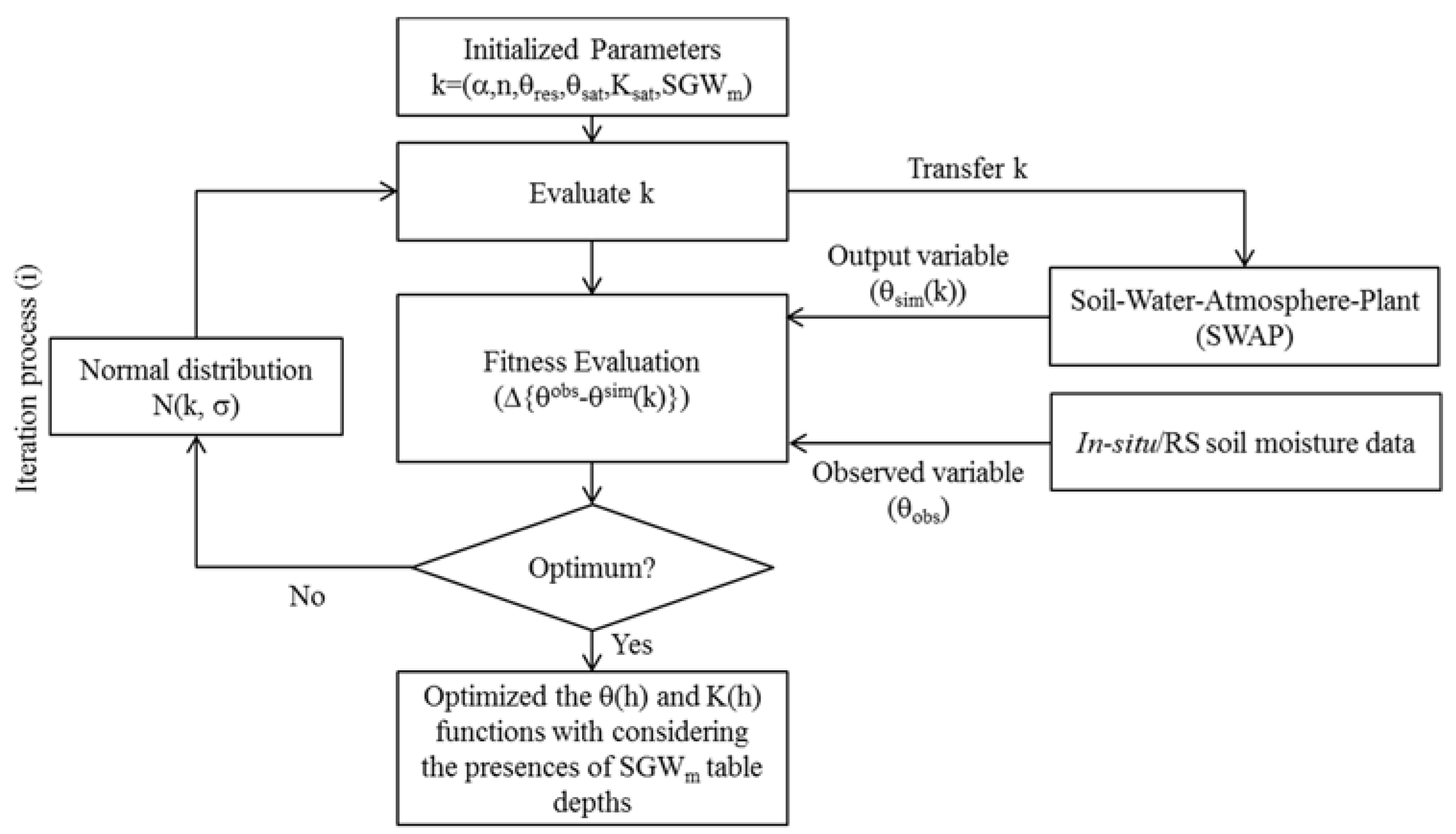
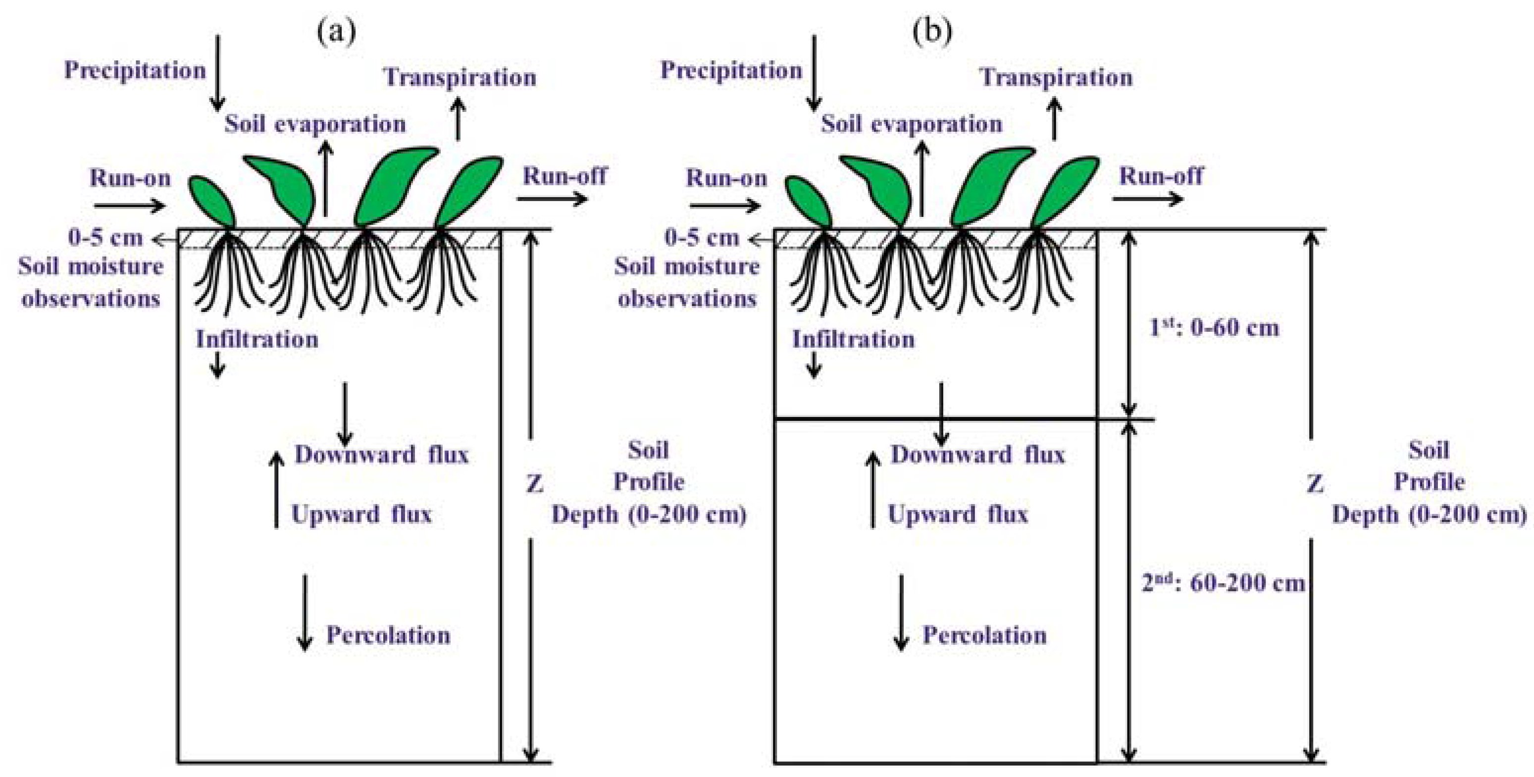
2.1. Conceptual Framework of the Dynamic Ground Water (DGW) Data Assimilation Approach

We developed a dynamic ground water (DGW) data assimilation scheme that can consider SGW oscillations in time for predicting the effective soil hydraulic properties (α, n, θ_res, θ_sat, K_sat) that determine the soil water content (θ(h)) and hydraulic conductivity (K(h)) in soils from RS soil moisture footprints. DGW adapts a near-surface soil moisture data assimilation scheme [6] based on an inversion model. Figure 1 shows the schematic diagram of our proposed approach. The DGW scheme is integrated with a soil–water–atmosphere–plant (SWAP) [20] model that simulates root zone soil moisture dynamics with the model input variables (e.g., soil parameters, vegetation, SGW table depths, weather forcings). Our DGW data assimilation scheme provides not only the soil parameters, but also the dynamically changing SGW table depths (SGW_m) in time to the SWAP model, whereas existing data assimilation schemes only estimate the soil parameters with the fixed SGW table depths across time in their modeling. The DGW approach adapts a newly developed optimization scheme (Iteration Algorithm-IA) for searching the optimized input variables (k = {α, n, θ_res, θ_sat, K_sat, SGW_{m = 1, …, M}}). Based on the objective function (Z(k)) in Equation (1), IA can provide the optimized model input variables (k) by minimizing the differences between the observed and simulated results.

$$Z(\text{k})=\text{min}\{\frac{1}{\mathrm{T}}{\displaystyle \sum _{\mathrm{t}=1}^{\mathrm{T}}({\mathsf{\theta }}_{\mathrm{t}}^{\text{obs}}-{\mathsf{\theta }}_{\mathrm{t}}^{\text{sim}}(\text{k})}\}$$

(1)

where ${\mathsf{\theta }}_{\mathrm{t}}^{\text{obs}}$: the observed soil moisture with time (t), ${\mathsf{\theta }}_{\mathrm{t}}^{\text{sim}}$: the simulated soil moisture with time (t), t: the running index, T: the given time, and M: the total number of months during the simulation period (t = 1, …, T). Note that we only generate the monthly SGW dynamics (1st day for individual months).

2.2. Soil–Water–Atmosphere–Plant Model

We adapted the soil–water–atmosphere–plant (SWAP) model as a one-dimensional (1-D) physics-based hydrological model [20,21]. SWAP simulates water flow across soil, water, atmosphere, and plant systems at the near-surface and in the unsaturated zone. The SWAP model calculates water flow based on Richards’ equation (Equation (2)). Van Genuchten [22] and Mualem [23] derived the soil hydraulic functions in the soil profile based on the analytical expression by considering the relationship between the water content (θ), pressure head (h), and unsaturated hydraulic conductivity (K).

$$\frac{\partial \mathsf{\theta }}{\partial \mathrm{t}}=\text{C}(h)\frac{\partial \mathrm{h}}{\partial \mathrm{t}}=\frac{\partial [\text{K}(\text{h})(\frac{\partial \mathrm{h}}{\partial \mathrm{z}}+1)]}{\partial \mathrm{z}}-S(h)$$

(2)

where θ: the volumetric water content (cm³·cm⁻³), K: the hydraulic conductivity (cm·d⁻¹), h: the soil water pressure head (–cm), z: the vertical soil depth (cm) taken positively upward, t: the time, C: the differential soil water capacity (cm⁻¹), and S(h): the actual soil water extraction rate by plants (cm³ cm⁻³·d⁻¹) defined as Equation (3),

$$S(h)={\mathsf{\alpha }}_{\mathrm{w}}(h)\frac{T_{pot}}{Z_r}$$

(3)

where T_pot: the potential transpiration (cm·d⁻¹), Z_r: the rooting depth (cm), and α_w: a reduction factor as a function of h, which takes into account water deficit and oxygen stress [24]. Richards’ Equation (2), using the finite difference scheme described by Belmans et al. [25], allows the use of soil hydraulic databases and all kinds of management scenarios:

$${\mathrm{S}}_{\mathrm{e}}=\frac{\mathsf{\theta }(\text{h})-{\mathsf{\theta }}_{\text{res}}}{{\mathsf{\theta }}_{\text{sat}}-{\mathsf{\theta }}_{\text{res}}}={[\frac{1}{1+{\left|\mathrm{\alpha }\text{h}\right|}^{\mathrm{n}}}]}^{\mathrm{m}}$$

(4)

$$\text{K}(\text{h})={\mathrm{K}}_{\text{sat}}{\mathrm{S}}_{\mathrm{e}}^{\mathsf{\lambda }}{[1-{(1-{\mathrm{S}}_{\mathrm{e}}^{1/\mathrm{m}})}^{\mathrm{m}}]}^2$$

(5)

where S_e: the relative saturation (-); θ_res: the residual water content (cm³·cm⁻³) in the dry range; θ_sat: the saturated water content (cm³·cm⁻³), α, n, m; λ: the shape parameters; K_sat: the saturated hydraulic conductivity (cm·d⁻¹); and m = 1 − 1/n.

In the SWAP model, we can determine the top (atmospheric) and bottom boundary (free drainage and SGW table depths) conditions. Also, it adapts the simple and detailed (WOFOST) crop growth routines combined with various water management modules (i.e., irrigation and drainage) that can consider the impacts of climate, soil textures, plant types, and crop water management [20,26]. SWAP, by adapting the Penman–Monteith equation, estimates the potential and actual soil evaporation (E_pot and E_act). Then, the potential and actual plant transpirations (T_pot and T_act) can be partitioned based on the leaf area index (LAI) or soil cover fraction (SC) of the land unit. The SWAP model is well-validated in performing under various climatic and environmental conditions [27,28,29,30,31].

2.3. Iteration Algorithm

The iteration algorithm (IA) was developed to generate the approximate solution (k = {α, n, θ_res, θ_sat, K_sat, SGW_{m = 1, …, M}) closer to the observation. In the IA scheme, the random variables (comprised of the soil hydraulic properties and SGW) are obtained via the normal distribution (N (k,σ)) with the mean (k) and standard deviation (σ = 0.5). The constraints for the randomly generated variables are shown in

Table 1. Maximum and minimum parameter constraints used in the iteration algorithm (IA).

Ranges	α	n	θres	θsat	Ksat	SGWm = 1, …, M
Max.	0.006	1.200	0.061	0.370	1.840	50.000
Min.	0.033	1.610	0.163	0.550	130.000	300.000

Notes: Iteration number (i): 3000; idum (initial random seed number): −1000; standard deviation (SD): 0.5 (synthetic condition)/0.8 (field validation); resampling number (n): 100.

. The IA always remembers the best solution through the given iteration processes (i), and the new random variables are generated from the previous best solution. Once the final solution in the given iterations (i = 1, …, I) was found, we applied the Monte Carlo (MC) resampling (ensemble, e = 100) technique based on the normal distribution to the best solution (k) in the iteration (i = I) to generate the uncertainty boundaries. In order to evaluate the model outputs, we calculated the Pearson’s correlation (R) using Equation (6) and root mean square error (RMSE) using Equation (7):

$$\mathrm{R}=\frac{{\displaystyle \sum _{\mathrm{t}=1}^{\mathrm{T}}({\mathsf{\theta }}_{\mathrm{t}}^{\text{obs}}-{\overline{\mathsf{\theta }}}^{\text{obs}})({\mathsf{\theta }}_{\mathrm{t}}^{\text{sim}}-{\overline{\mathsf{\theta }}}^{\text{sim}})}}{\sqrt{{\displaystyle \sum _{\mathrm{t}=1}^{\mathrm{T}}{({\mathsf{\theta }}_{\mathrm{t}}^{\text{obs}}-{\overline{\mathsf{\theta }}}^{\text{obs}})}^2}{\displaystyle \sum _{\mathrm{t}=1}^{\mathrm{T}}{({\mathsf{\theta }}_{\mathrm{t}}^{\text{sim}}-{\overline{\mathsf{\theta }}}^{\text{sim}})}^2}}}$$

(6)

$$\text{RMSE}=\sqrt{\frac{{\displaystyle \sum _{\mathrm{t}=1}^{\mathrm{T}}{({\mathsf{\theta }}_{\mathrm{t}}^{\text{obs}}-{\mathsf{\theta }}_{\mathrm{t}}^{\text{sim}})}^2}}{\mathrm{T}}}$$

(7)

where e: the total number of ensembles, ${\overline{\mathsf{\theta }}}_{\mathrm{t}}^{\text{obs}}$: the average observed soil moisture with time (t), and ${\overline{\mathsf{\theta }}}_{\mathrm{t}}^{\text{sim}}$: the average simulated soil moisture with time (t).

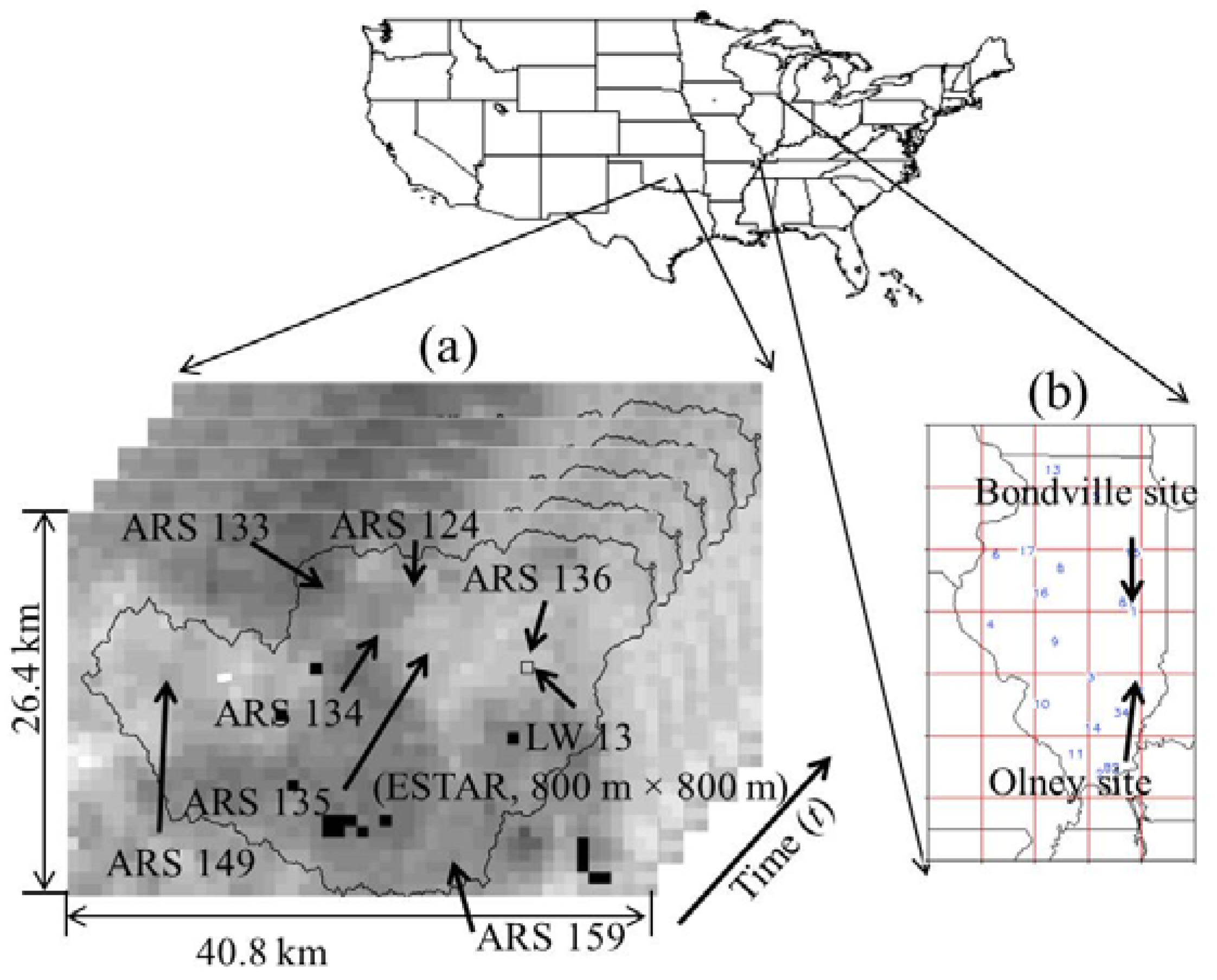
2.4. Description of Study Sites and Data

We selected the Little Washita 13 (LW 13) site in Oklahoma and the Olney (OLN)/Bondville (BOND) sites in Illinois to test our proposed DGW scheme (Figure 2). The in situ soil moisture (0–10 cm) data (13/12 days for OLN/ BOND in 2004/2003, respectively) and measured ground water table depths were provided by the International Soil Moisture Network (ISMN) [32], but no ground water table depth information was available at the LW 13 site. The Water and Atmospheric Resources Monitoring Program (WARMP), part of the Illinois State Water Survey (ISWS) located in Champaign and Peoria (Illinois), provided the daily measured SGW table depths for the OLN/BOND sites. The airborne sensing scale (800 m × 800 m) electronically scanned thinned array radiometer (ESTAR) [33] soil moisture (5 cm) products were taken for 17 days during the Southern Great Plains experiment (SGP97, from 18 June to 18 July) in 1997 at the LW watershed. The currently available satellite-scale Advanced Microwave Scanning Radiometer–Earth (AMSR–E) [34] platform only provides the near-skin (0–1/0–2 cm) soil moisture, indicating that it is limited in representing root zone soil moisture dynamics at the field. For this reason, we aggregated the ESTAR soil moisture (33 rows × 51 columns) to consider the satellite scale. Considering that the soil moisture active passive (SMAP) mission [35] provides near-surface (0–5 cm) soil moisture footprints, we assumed that the aggregated ESTAR data can represent the satellite-scale soil moisture. The LW 13 and OLN/BOND sites are composed of predominantly loam and silt loam soils (ISMN) [36] with grass cover. The daily weather information (i.e., precipitation, wind speed, maximum and minimum temperature, and solar radiation) for the input parameters to the SWAP model were collected from the USDA Agricultural Research Service (ARS 136 for the LW 13 site, ARS 149 for the LW 21 site, and ARS 133, 134, 146, and 149 for the LW site) [37] Micronet weather station in Oklahoma and the Illinois State Water Survey (ISWS) [38]. Also, we validated our approach using the field-observed hydraulic parameters [36] obtained from the soil core samples at the soil depth (3–9 cm) at the LW 13 site.

2.5. Numerical

We conducted the numerical experiments to assess the DGW data assimilation scheme at the point, airborne sensing, and satellite scales under various hydroclimatic conditions. In order to test the performance of our proposed scheme, we compared model outputs of the DGW scheme to those derived by the original near-surface data assimilation considering the fixed (given) ground water (FGW) table depth (e.g., −300, −200, −100 cm) in time. Here, the near-surface data assimilation with the FGW table depths is named the FGW scheme. The numerical experiments were comprised of two conditions under rain-fed conditions: (i) synthetic and (ii) field validation conditions. For the synthetic condition, we generated the root zone soil moisture using the existing input data (i.e., soil textures, vegetation, weather forcings, and SGW table depths) to SWAP in a forward mode. Note that the generated soil moisture dynamics were defined as the synthetic root zone soil moisture observations. Then, the DGW and FGW approaches derive the soil hydraulic properties from the synthetic observations, and the root zone soil moisture estimates based on the derived soil parameters were compared to the synthetic observations. Thus, the synthetic condition can test its own performances of DGW and FGW approaches by excluding factors such as measurement errors and model structural uncertainties. Here, we selected three different soil textures (Sandy Loam–SL, Silt Loam–SiL, and Clay Loam–CL soils) and grass cover with weather data provided by the ARS 136 site, and a soil column (0–200 cm) assumed to be a homogeneous soil layer (Figure 3a). The references of laboratory-based soil texture information (SL, SiL, and CL) were obtained from the UNSODA database [39]. Under the synthetic conditions, we tested the performance of the FGW and DGW schemes in parameter estimations with various fixed SGW table depths of −100, −200, and −300 cm from the soil surface. Based on the estimated soil parameters, we compared the water retention (θ(h)) and hydraulic conductivity (K(h)) curves. Furthermore, we tested the FGW and DGW approaches with various vegetation covers (grass, wheat, maize, and soybean) and silt loam soil with the dynamically changing SGW tables of −160.0, −200.0, −170.0, −170.0, −170.0, −170.0, and −160.0 cm (1st day for individual months, April–October). Generally, the inversion model scheme predicts the effective soil hydraulic properties that can represent the entire soil domain vertically using only the near-skin (0–1/0–5 cm) soil moisture data. However, the heterogeneity (e.g., soil textures, soil layers) in the soil column influence the soil parameter estimations considerably [40]. In order to test the performance of the DGW model with soil heterogeneity, we designed a layered soil column comprised of two layers (1st: silt loam-SiL soil and 2nd: loam-L soil at the soil depths of 0–60 and 60–200 cm, respectively), as shown in Figure 3b. In the field validation experiments, the FGW and DGW schemes were evaluated with in situ, airborne-scale, and satellite-scale soil moisture data at multiple scales.

3. Results and Discussion

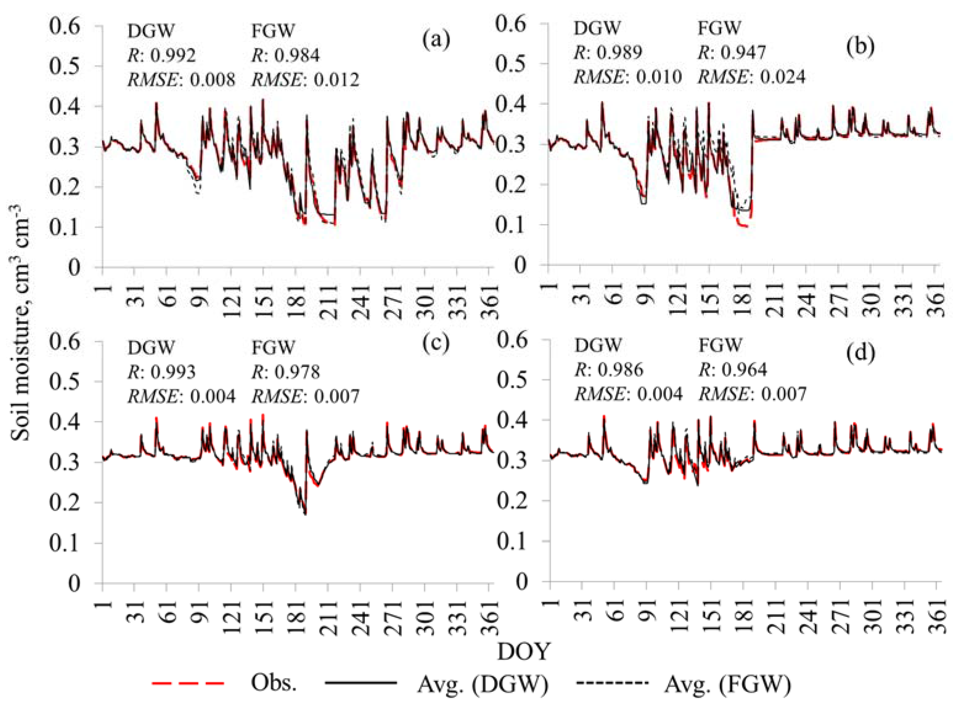
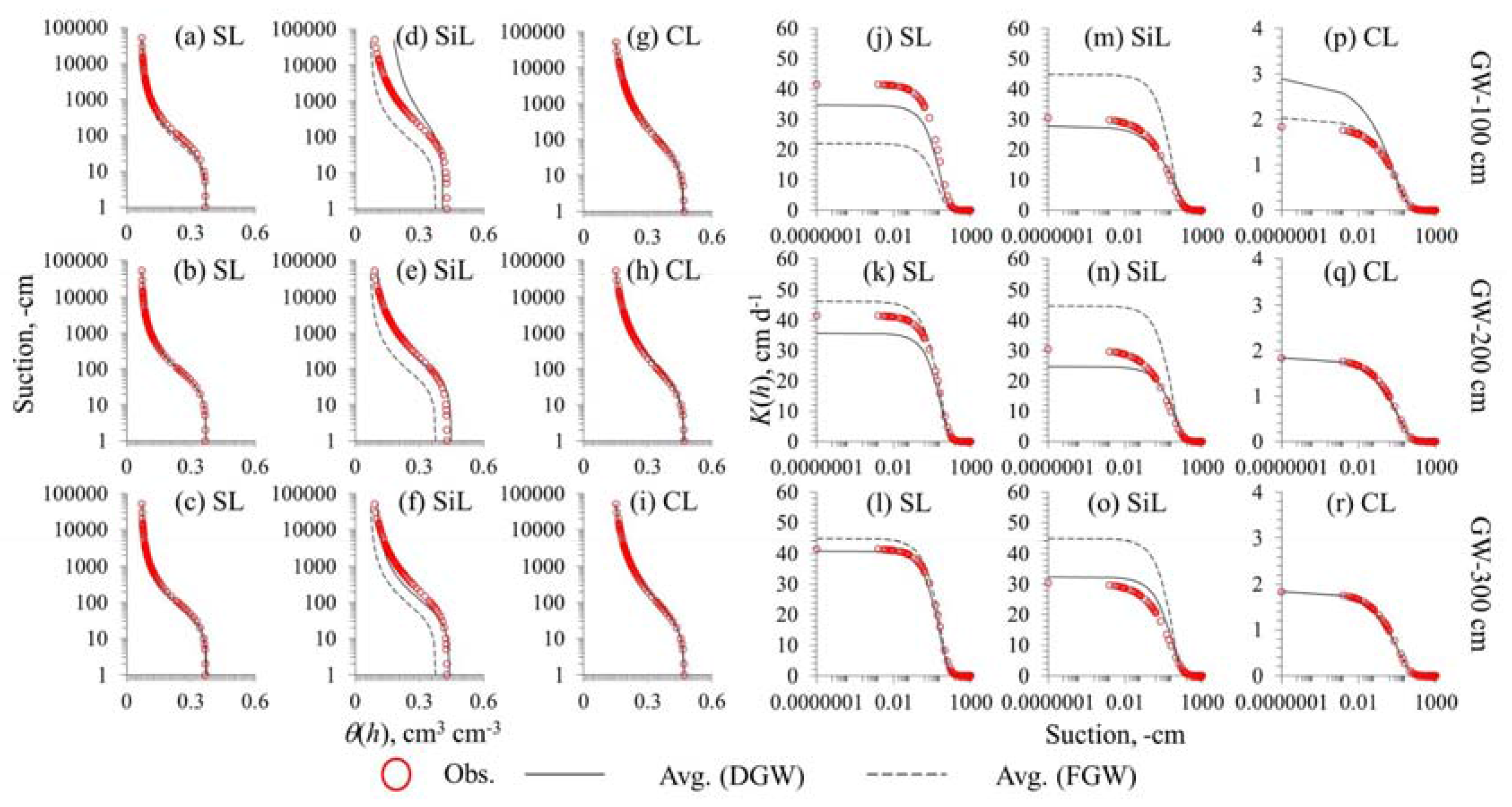
3.1. Synthetic Conditions

We tested the newly developed DGW scheme that can consider dynamically changing shallow ground water tables for predicting the soil hydraulic properties under the synthetic conditions. Figure 4 shows the water retention (θ(h)) and hydraulic conductivity (K(h)) curves using the estimated soil parameters based on the FGW (dashed line) and DGW (thin line) approaches for different soils (SL, SiL, and CL) with SGW table depths (no oscillations in time) of −300, −200, and −100 cm. The FGW- and DGW-based θ(h) curves for sandy loam and clay loam soils generally matched the observations with the presence of SGW tables, while the results for silt loam soil showed small uncertainties, especially for the FGW scheme. The K(h) curves usually had more uncertainties than those of the θ(h) curves as the SGW tables come closer to the soil surface. However, the DGW-based K(h) curves consistently were in good agreement with the observations, with small uncertainties compared to those of FGW, although the result of DGW for clay loam soil with GW −100 cm was slightly more biased. Overall, the hydraulic conductivities (K(h)) were sensitive to the presence of SGW tables compared those of θ(h). This might provide significant inferences with respect to parameterization schemes adapting physics-based hydrological models because these parameters limit soil moisture dynamics in the root zone. Thus, the presence of SGW tables considerably influences the physical flow processes (directly related to K(h)) occurring in the soil profile [9,40]. Although the derived θ(h) and K(h) curves had uncertainties (especially for silt loam soil), the DGW data assimilation approach performed better for estimating the soil hydraulic properties than FGW with various SGW table depths.

Figure 5 shows the comparison of observed (synthetic) and simulated root zone soil moisture dynamics using the FGW and DGW schemes with silt loam soil and various vegetation covers (grass, wheat, soybean, and maize) under the conditions of dynamically changing SGW tables at the ARS 136 site in Oklahoma (1997). As shown in the findings in Figure 4, the DGW-based results (R: 0.986−0.993 and RMSE: 0.004−0.010) matched the synthetic observations better than those of FGW (R: 0.947−0.984 and RMSE: 0.007−0.024). Also, the model outputs showed that soybean and maize can hold more moisture than grass and wheat.

Table 2. Observed and simulated soil hydraulic properties at Agricultural Research Service (ARS) 136 site in Oklahoma (1997) with silt loam soil and various vegetation covers under synthetic conditions.

Silt Loam (Target Values)			α	n	θres	θsat	Ksat
			0.012	1.39	0.061	0.43	30.5
Grass	DGW	Avg.	0.013	1.456	0.106	0.431	27.948
		SD	0.001	0.026	0.005	0.017	0.801
	FGW	Avg.	0.015	1.401	0.075	0.405	12.85
		SD	0.001	0.008	0.002	0.003	0.810
Wheat	DGW	Avg.	0.014	1.45	0.115	0.431	31.81
		SD	0.001	0.026	0.005	0.017	0.801
	FGW	Avg.	0.015	1.42	0.087	0.402	14.019
		SD	0.001	0.008	0.002	0.003	0.810
Soybean	DGW	Avg.	0.014	1.384	0.137	0.411	29.843
		SD	0.001	0.026	0.005	0.017	0.801
	FGW	Avg.	0.021	1.325	0.13	0.397	19.894
		SD	0.001	0.008	0.002	0.003	0.810
Maize	DGW	Avg.	0.014	1.456	0.139	0.423	32.056
		SD	0.001	0.026	0.005	0.017	0.801
	FGW	Avg.	0.018	1.414	0.107	0.41	18.296
		SD	0.001	0.008	0.002	0.003	0.81
Grass (Layered soil column)	DGW	Avg.	0.009	1.471	0.064	0.462	26.914
		SD	0.001	0.026	0.005	0.017	0.801
	FGW	Avg.	0.016	1.41	0.07	0.394	11.285
		SD	0.000	0.008	0.002	0.003	0.810

Notes: DGW: Dynamic Ground Water data assimilation; FGW: Fixed Ground Water data assimilation. UNSODA database [39].

shows the statistics of soil hydraulic properties (used in Figure 5) derived by the FGW and DGW schemes with the references (as target values) of soil texture information [39]. Comparing the estimated soil parameters to the results as shown in Figure 5, the FGW approach, showed relatively higher uncertainties with the SGW dynamics, especially for the values of K_sat (12.850–19.894 mm·d⁻¹). The K_sat values were usually underestimated compared to the target value of silt loam soil (30.500 mm·d⁻¹), while the DGW scheme still estimated soil parameter values (i.e., K_sat in the ranges of 27.948–32.056 mm·d⁻¹) that are closer to the target value. Furthermore, the estimated DGW tables were identifiable in the observations with small uncertainties, as shown in

Table 3. Monthly observed (target values) and simulated shallow ground water table depths at ARS 136 site in Oklahoma (1997) with silt loam soil and various vegetation covers under synthetic conditions.

Date	Target Values (Obs. SGW, cm)	Grass		Wheat		Soybean		Maize		Grass (Layered Soil Column)
		Avg.	SD	Avg.	SD	Avg.	SD	Avg.	SD	Avg.	SD
04-01	160.0	149.9	7.4	154.4	7.4	162.9	7.4	155.5	7.4	170.0	7.4
05-01	200.0	208.1	13.2	200.8	13.2	202.0	13.2	186.0	13.2	196.3	13.2
06-01	170.0	152.4	5.3	168.8	5.3	173.4	5.3	162.2	5.3	174.3	5.3
07-01	170.0	171.3	4.3	159.9	4.3	151.6	4.3	171.4	4.3	186.9	4.3
08-01	170.0	159.3	5.5	175.1	5.5	179.3	5.5	163.8	5.5	188.0	5.5
09-01	170.0	157.5	7.6	176.8	7.6	181.2	7.6	169.6	7.6	211.4	7.6
10-01	160.0	145.2	6.9	144.9	6.9	161.8	6.9	152.1	6.9	172.3	6.9

. These findings might support the robustness of DGW data assimilation for considering the SGW dynamics with time, although these numerical studies were conducted under synthetic conditions.

We tested our proposed approach in the layered soil column comprised of two soil textures (1st layer: silt loam soil and 2nd layer: loam soil) as shown in Figure 6. The comparison of observed and estimated root zone soil moisture dynamics in the 1st layer (0–60 cm) in the DGW scheme showed good agreement (R: 0.988 and RMSE: 0.009), while the FGW-based results had more uncertainties (R: 0.915 and RMSE: 0.025). The DGW approach (R: 0.474 and RMSE: 0.042) estimated the deep soil moisture dynamics better than those of the FGW (R: −0.173 and RMSE: 0.037) in the 2nd layer (60–200 cm), although higher uncertainties exist in both results. These findings show that the increased number of unknown parameters (e.g., soil layers, different soil textures) in the soil column causes higher uncertainties in the parameter estimations based on the inverse modeling. Considering that the sub-surface layer in field regions is usually heterogeneous because of different soil layers and soil textures, the near-surface soil moisture data assimilation scheme could be limited in predicting vertical soil water flow across the whole soil profile using only the near-surface soil moisture information. However, the DGW assimilation scheme improved the estimated soil parameters in the layered column better than those of the FGW scheme. The DGW-based soil parameters (see Table 2) and SGW tables (see Table 3) in the layered soil column also matched the observations with predictable uncertainties. Thus, the newly developed DGW data assimilation scheme could improve upon the limitations due to the heterogeneity along the soil profile in estimating the soil hydraulic properties in fields. When we considered that the environmental factors (e.g., soil textures, presence of SGW tables, layers, root depth and distribution) are unknown in field conditions, our approach could provide more reliable model outputs in fields with small uncertainties.

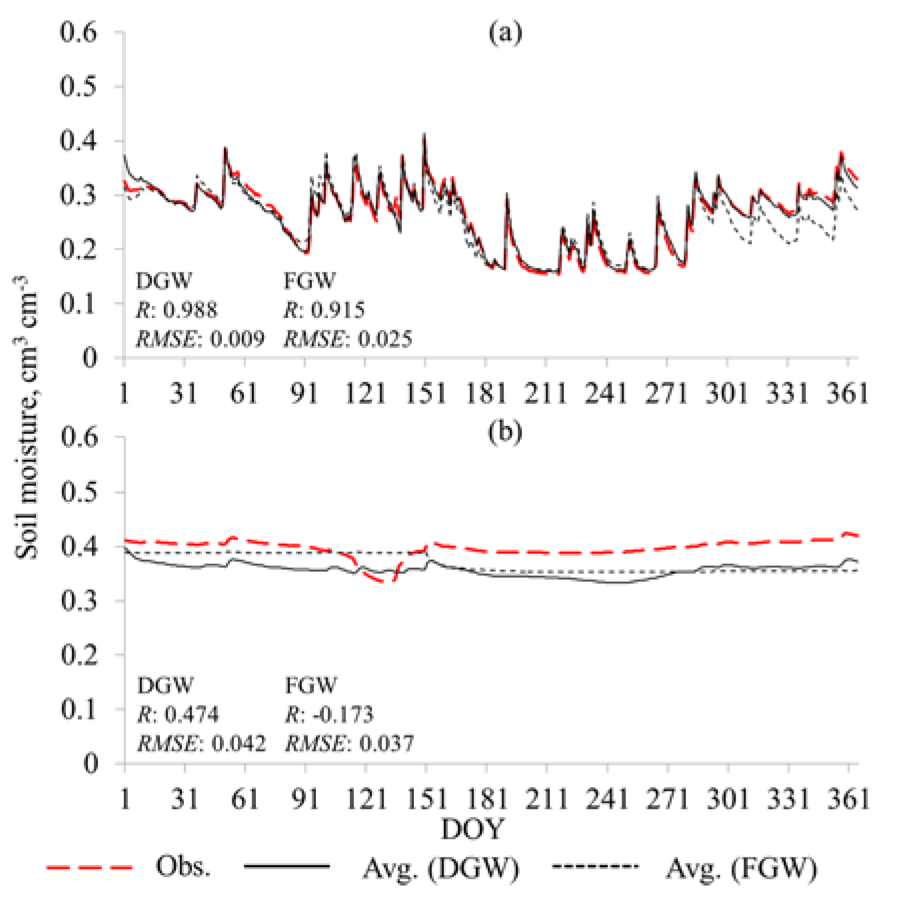
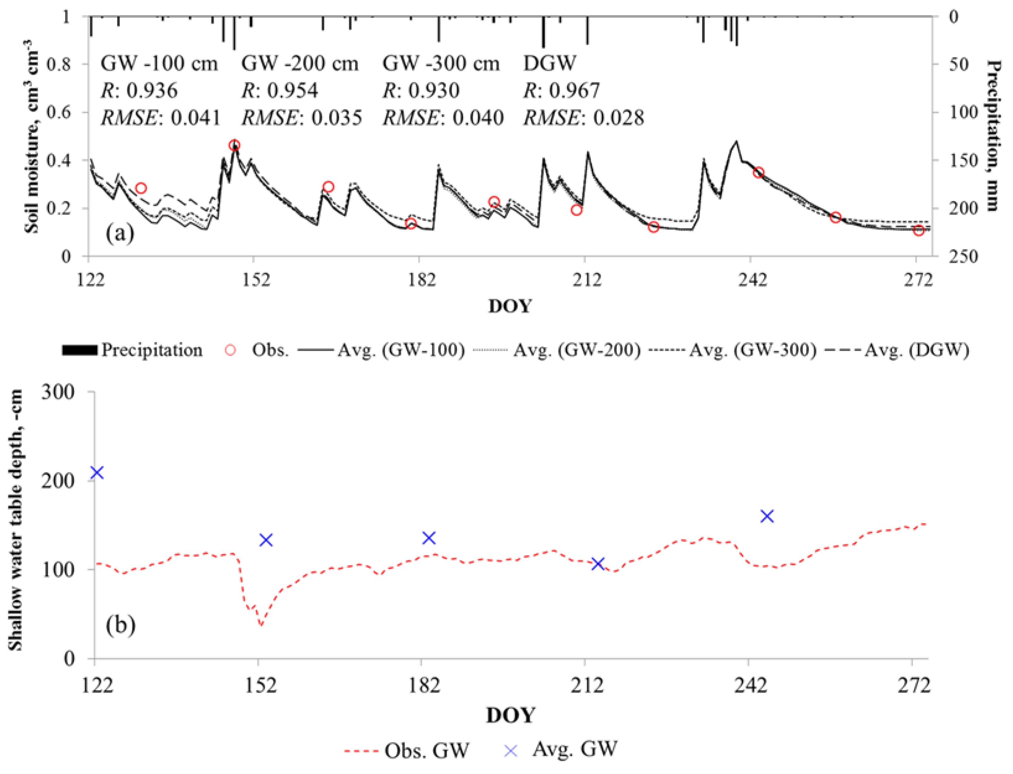
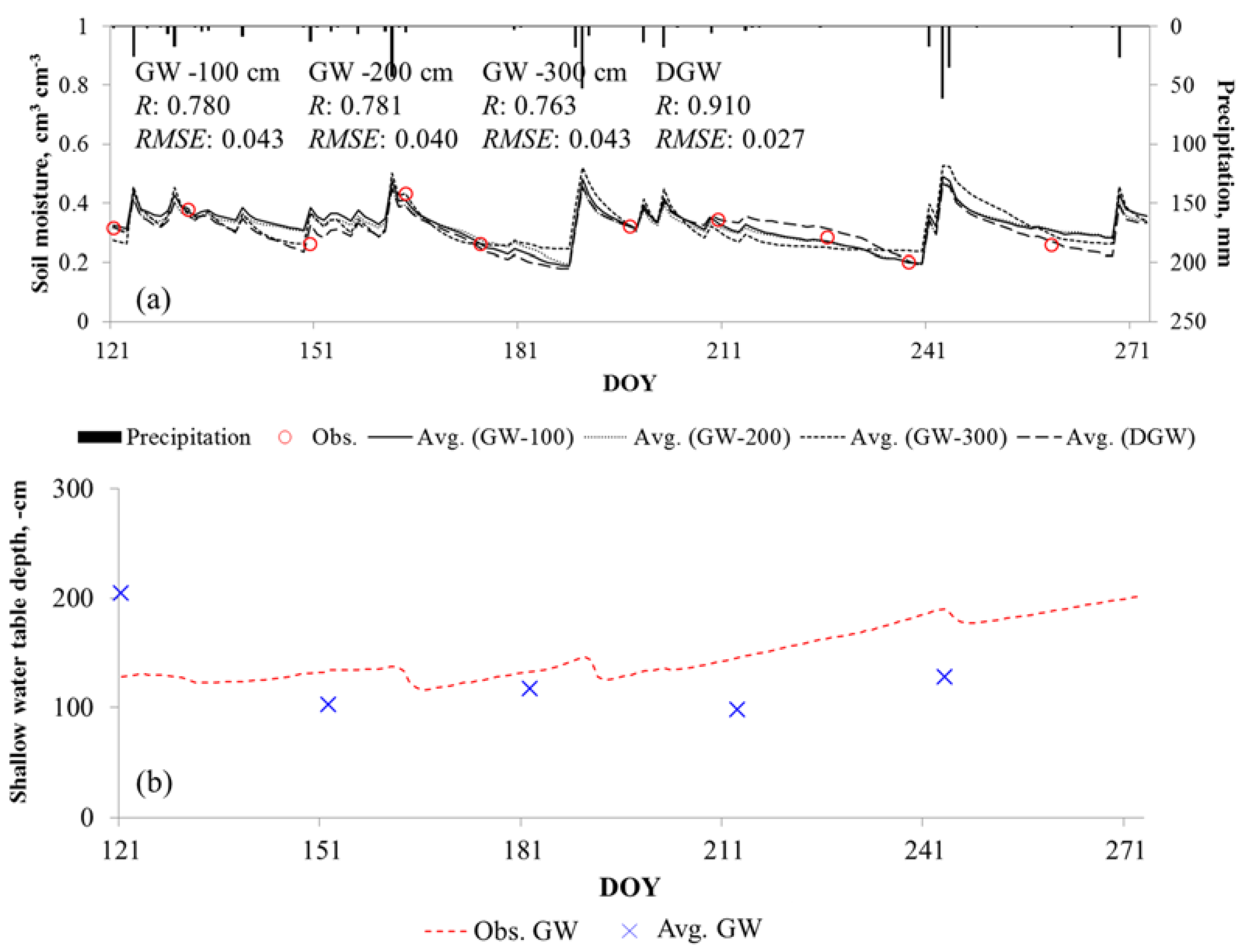
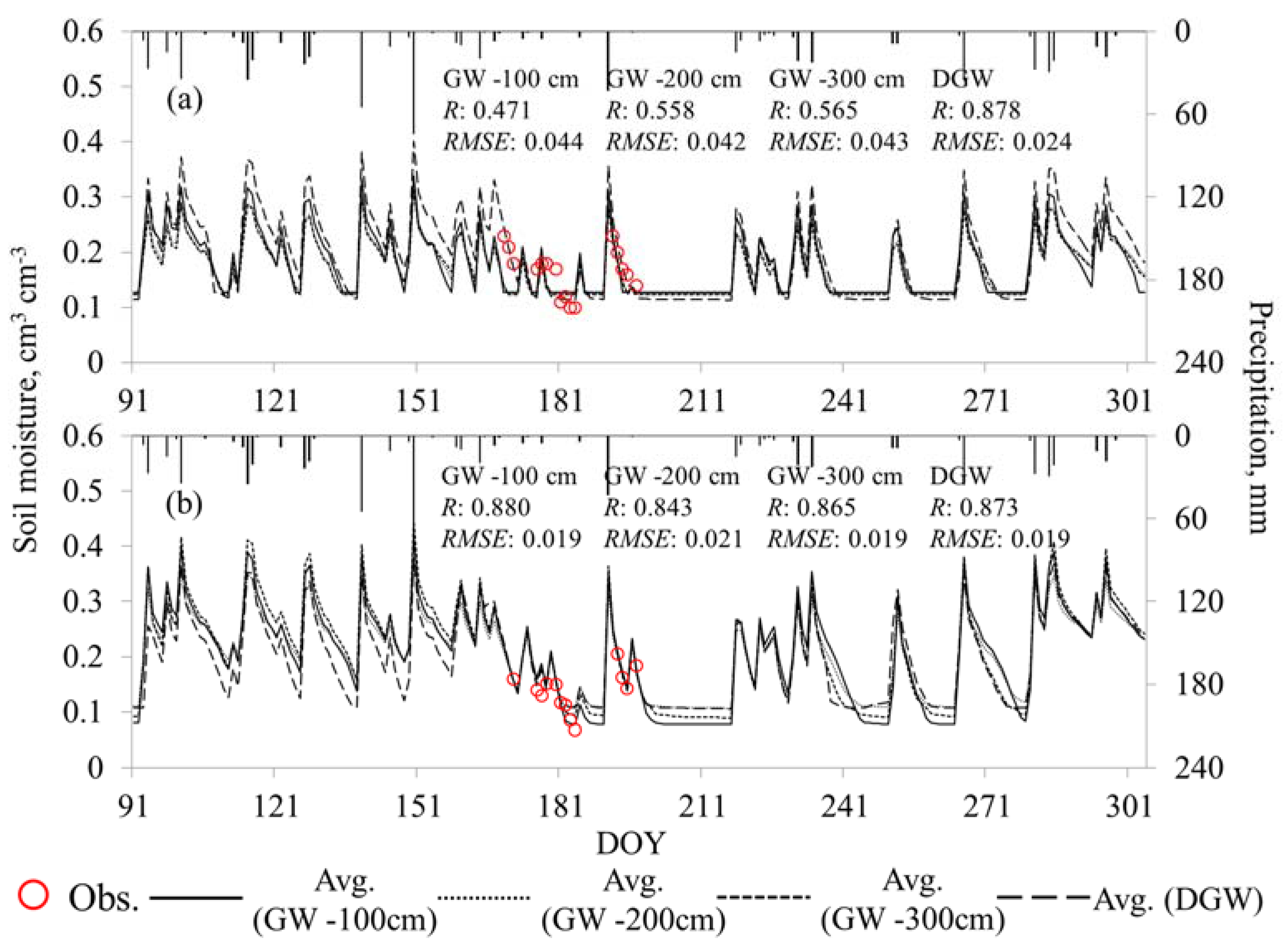
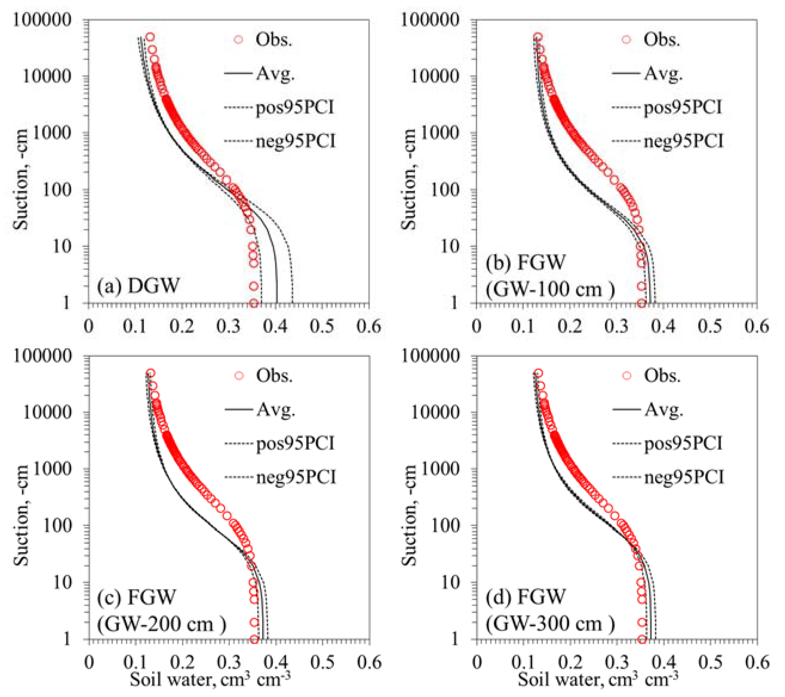
3.2. Field Validation Experiments

The DGW scheme was validated at the BOND (2004) and OLN (2003) sites in Illinois with the measured soil moisture and shallow ground water table dynamics. As shown in the results with synthetic conditions, our approach performed well in reproducing the simulated root zone soil moisture and SGW dynamics as shown in Figure 7a. The correlation (R: 0.967) and RMSE (0.028) for DGW (OLN) were considerably improved compared to those (R: 0.930, 0.954, 0.933 and RMSE: 0.040, 0.035, 0.041) for FGW, with fixed SGW table depths of −300, −200, and −100 cm. The differences in soil moisture estimates derived by the DGW and FGW schemes increased during dry days, while the results showed similar trends for wet periods. This indicated that the soil parameter estimations are affected by the SGW table fluctuations and recharged, with time, by precipitation. Figure 7b shows the comparison of measured and estimated SGW table dynamics. The measured SGW tables change with time based on the rainfall amounts/frequencies. As the rainfall events were generated, the measured soil moisture values increased. Also, the SGW table depths became higher (closer to the soil surface). Although the SGW tables estimated by the DGW scheme were relatively underestimated (more negative from the soil surface) during the initial simulation period compared to the measurements, these model outputs followed the measured SGW data.

Figure 8 shows the validated root zone soil moisture and SGW dynamics at the BOND site. These also showed trends similar to the DGW-based model outputs (R: 0.910 and RMSE: 0.027) and are more identifiable from the measurements than those of the FGW scheme (R: 0.763−0.781, RMSE: 0.040−0.043). The estimated SGW depths during the initial simulation periods (Day-of-Year (DOY) 121) were overestimated compared to the measurements shown in Figure 7b. The nighttime temperature (DOY 1–90) in Illinois is usually below zero degrees (°C), and the snow melting or thawing effect on the soil column might influence the measured ground water depths (relatively higher values compared to the simulation results). However, the SWAP model has no module that can simulate these physical processes in modeling. Thus, uncertainties in the estimated SGW table depths during the initial periods for the BOND and OLN sites might be due to both the measurements and model structural errors. Overall, our proposed scheme estimated the soil moisture dynamics and SGW table depths during the simulation period quite well, except for during the initial days.

Figure 9a,b present the comparison of estimated root zone soil moisture dynamics using the FGW and DGW data assimilation schemes at the ESTAR airborne (800 m × 800 m for a pixel) and satellite (33 rows × 51 columns for the aggregated pixels) scales within the LW watershed in Oklahoma. The root zone soil moisture estimates (R: 0.471, 0.558, 0.565 and RMSE: 0.044, 0.042, 0.043 for GW −100, −200, and −300 cm, respectively) by the FGW scheme had relatively larger uncertainties than those of DGW (R: 0.878 and RMSE: 0.024). The satellite-scale model outputs also showed similar results. The estimated root zone soil moisture dynamics (R: 0.873 and RMSE: 0.019) identified with the aggregated ESTAR products better than those of FGW (R: 0.880, 0.843, 0.865 and RMSE: 0.019, 0.021, 0.019 for GW at −100, −200, and −300 cm), except for the correlation (R: 0.873) of GW at −100 cm. In order to validate the estimated soil parameters, we compared the observed and derived water retention curves (θ(h)) at the airborne scale (LW 13) as shown in Figure 10. Note that the observed θ(h) curve was derived by the field-scale soil hydraulic properties [36] taken from the soil core (3–9 cm) at the LW 13 site in 1997. The estimated θ(h) curves were usually biased from the observation, especially those of GW at −100 and −200 cm. The θ(h) curves with DGW and FGW (GW at −300 cm indicating relatively free-drainage conditions) were closer to the observation. When we considered that the LW 13 site has a hill slope at the airborne sensing scale, the DGW-based θ(h) curve might be comparable with that of FGW (GW at −300 cm).

4. Conclusions

In this study, we developed a dynamic ground water (DGW) data assimilation scheme that can consider SGW table depth dynamics across time in the unsaturated zone at the point, airborne, and satellite scales in various hydroclimatic regions. The DGW scheme adapts a near-surface soil moisture data assimilation scheme [6] that can quantify the pixel-scale soil hydraulic properties (α, n, θ_res, θ_sat, K_sat) from RS soil moisture footprints. Note that this near-surface soil moisture data assimilation scheme adapting the physics-based soil–water–atmosphere–plant (SWAP) model only considers the fixed SGW table depths in time, and was named the fixed ground water (FGW) data assimilation scheme. Our proposed DGW scheme can derive not only the soil parameters, but also monthly SGW table depth dynamics in time from RS data. The newly developed simple iteration algorithm (IA) was integrated with the DGW data assimilation for searching the optimized soil parameters and time-variant SGW table depths by minimizing the differences between the observed and SWAP-based soil moisture dynamics. In order to verify our approach, numerical experiments comprised of the synthetic conditions and field validation experiments were conducted. For the numerical studies, the Little Washita (LW) watershed in Oklahoma and Olney (OLN)/Bondville (BOND) sites in Illinois, which are in different hydroclimatic regions, were selected. The synthetic studies were conducted using the weather data at the ARS 136 site and laboratory-based soil textures [39] within the LW watershed, and field validations were conducted at the ONL and BOND sites.

For the synthetic conditions, we tested the FGW and DGW data assimilation schemes with various soil textures (sandy loam–SD, silt loam–SiL, clay loam–CL, and loam–L, UNSODA database [39]) and vegetation covers (grass, wheat, soybean, and maize) with the fixed and dynamically changing SGW table depths in homogeneous and heterogeneous (layered) soil columns across time. Under the fixed SGW table depths of −300, −200, and −100 cm for individual SL, SiL, and CL soils, the FGW and DGW approaches derived the effective soil hydraulic properties from the synthetic near-surface (0–5 cm) soil moisture dynamics at the ARS 136 site. The water retention curves (θ(h)) derived by the DGW-based estimated soil parameters matched the observations, while the θ(h) curves from the FGW scheme showed uncertainties for SiL soil. The FGW-based hydraulic conductivities (K(h)) were highly biased compared to the observed curves, indicating that the presence of SGW table depths considerably influence the K_sat variable. However, the K(h) functions derived by our proposed approach usually showed a good agreement with the synthetic observations. In the layered soil system (1st and 2nd layers at soil depths of 0–60 and 60–200 cm with SiL and L soils, respectively), the DGW-based data assimilation still performed better in estimating the soil parameters compared to those based on the FGW scheme. In the field validations, the FGW and DGW schemes usually showed good model performances, but the DGW-based model outputs showed better correlations (R) and smaller uncertainties (RMSE). Although we only validated the monthly estimated SGW table depths to the measured data at the point scale (BOND/OLN), our proposed model can provide improved root zone (0–10 cm) soil moisture dynamics with small uncertainties better than those of FGW at the study sites. The airborne sensing- and satellite-scale soil moisture estimates in the DGW scheme also identified slightly better with the ESTAR soil moisture products compared to those of FGW. According to the studies of Ines and Mohanty [6] and Shin et al. [9,40], the presence of SGW table depths in the unsaturated zone considerably influences the soil parameter estimations. The proposed DGW scheme that can consider both the soil hydraulic properties and SGW table depth dynamics in time performed well for the synthetic and field validation, supporting the robustness of our approach in application to field regions. Thus, our approach could improve the availability and applicability of pixel-scale soil moisture footprints based on satellite platforms.

References

1. Kerr, Y.H.; Waldteufel, P.; Wigneron, J.P.; Martinuzzi, J.M.; Font, J.; Berger, M. Soil moisture retrieval from space: The soil moisture and ocean salinity (SMOS) mission. IEEE Trans. Geosci. Remote Sens. 2001, 39, 1729–1735. [Google Scholar] [CrossRef]
2. Njoku, E.G.; Jackson, J.J.; Lakshmi, V.; Chan, T.K.; Nghiem, S.V. Soil moisture retrieval from AMSR-E. IEEE Trans. Geosci. Remote Sens. 2003, 41, 215–229. [Google Scholar] [CrossRef]
3. Entekhabi, D.; Njoku, E.G.; Houser, P. The Hydrosphere State (Hydros) mission: An Earth system pathfinder for global mapping of soil moisture and land freeze/thaw. IEEE Trans. Geosci. Remote Sens. 2004, 42, 2184–2195. [Google Scholar] [CrossRef]
4. Ottlé, C.; Vidal-Madjar, D. Assimilation of soil moisture inferred from infrared remote sensing in a hydrological model over the HAPEX-MOBILHY region. J. Hydrol. 1994, 158, 241–264. [Google Scholar] [CrossRef]
5. Njoku, E.; Entekkabi, D. Passive microwave remote sensing of soil moisture. J. Hydrol. 1996, 184, 101–129. [Google Scholar] [CrossRef]
6. Ines, A.V.M.; Mohanty, B.P. Near-surface soil moisture assimilation to quantify effective soil hydraulic properties using genetic algorithm. I. Conceptual modeling. Water Resour. Res. 2008, 44. [Google Scholar] [CrossRef]
7. Ines, A.V.M.; Mohanty, B.P. Near-surface soil Moisture assimilation for quantifying effective soil hydraulic properties using genetic algorithms: II. Using airborne remote sensing dyring SGP97 and SMEX02. Water Resour. Res. 2008, 45. [Google Scholar] [CrossRef]
8. Ines, A.V.M.; Mohanty, B.P. Parameter Criterioning with a Noisy Monte Carlo Genetic Algorithm for Estimating Effective Soil Hydraulic properties from Space. Water Resour. Res. 2008, 44. [Google Scholar] [CrossRef]
9. Shin, Y.; Mohanty, B.P.; Ines, A.V.M. Estimating effective soil hydraulic properties using spatially distributed soil moisture and evapotranspiration. Vadose Zone J. 2013, 12. [Google Scholar] [CrossRef]
10. Galantowicz, J.F.; Entekhabi, D.; Njoku, E.G. Tests of sequential data assimilation for retrieving profile soil moisture and temperature from observed L-band radiobrightness. IEEE Trans. Geosci. Remote Sens. 1999, 37, 1860–1870. [Google Scholar] [CrossRef]
11. Walker, J.P.; Willgoose, G.R.; Kalma, J.T. One-dimensional soil moisture profile retrieval by assimilation of near-surface observations: A comparison of retrieval methods. Adv. Water Resour. 2001, 24, 631–650. [Google Scholar] [CrossRef]
12. Crow, W.T.; Wood, E.F. The assimilation of remotely sensed soil brightness temperature imagery into a land surface model using enxemble Kalman filtering: A case study based on ESTAR measurements during SGP97. Adv. Water Resour. 2003, 26, 137–149. [Google Scholar] [CrossRef]
13. Dunne, S.; Entekhabi, D. An ensemble-based reanalysis approach to land data assimilation. Water Resour. Res. 2005, 41, W02013. [Google Scholar] [CrossRef]
14. Oleson, K.W.; Lawrence, D.M.; Bonan, G.B.; Flanner, M.G.; Kluzek, E.; Lawrence, P.J.; Levis, S.; Swenson, S.C.; Thornton, P.E. Technical Description of Version 4.0 of the Community Land Model. Available online: http://www.cesm.ucar.edu/models/cesm1.0/clm/CLM4_tech_Note.pdf (accessed on 5 December 2015).
15. Ek, M.; Mitchell, K.E.; Lin, Y.; Rogers, E.; Grunmann, P.; Koren, V.; Gayno, G.; Tarpley, J.D. Implementation of Noah land surface model advances in the National Centers for Environmental Prediction operational mesoscale Eta Model. J. Geophys. Res. 2003, 108, 8851. [Google Scholar] [CrossRef]
16. Vazquez-Amábile, G.G.; Engel, B.A. Use of SWAT to compute groundwater table depth and streamflow in the Muscatatuck river watershed. Trans. ASAE 2005, 48, 991–1003. [Google Scholar] [CrossRef]
17. Pivot, J.M.; Josien, E.; Martin, P. Farms adaptation to changes in flood risk: A management approach. J. Hydrol. 2002, 267, 12–25. [Google Scholar] [CrossRef]
18. Skaggs, R.W. DRAINMOD Reference Report; USDA Soil Conservation Service: Washington, DC, USA, 1980. [Google Scholar]
19. Arnold, J.G.; Srinavasan, R.; Muttiah, R.S.; Williams, J.R. Large-area hydrologic modeling and assessment: Part I. Model development. J. Am. Water Resour. Assoc. 1998, 34, 73–89. [Google Scholar] [CrossRef]
20. Van Dam, J.C.; Huygen, J.; Wesseling, J.G.; Feddes, R.A.; Kabat, P.; van Waslum, P.E.V.; Groenendijk, P.; van Diepen, C.A. Theory of SWAP Version 2.0: Simulation of Water Flow and Plant Growth in the Soil-Water-Atmosphere-Plant Environment; Technical Document 45; Wageningen Agricultural University and DLO Winand Staring Centre: Wageningen, The Netherlands, 1997. [Google Scholar]
21. Kroes, J.G.; van Dam, J.C.; Huygen, J.; Vervoort, R.W. User’s Guide of SWAP Version 2.0: Simulation of Water, Solute Transport, and Plant Growth in the Soil–Atmosphere–Plant Environment; Report 81; DLO Winand Staring Centre: Wageningen, The Netherlands, 1999. [Google Scholar]
22. Van Genuchten, M.T. A closed-form equation foe predicting the hydraulic conductivity of unsaturated soils. Soil Sci. Soc. Am. J. 1980, 44, 892–898. [Google Scholar] [CrossRef]
23. Mualem, Y. A new model for predicting the hydraulic conductivity of unsaturated porous media. Water Resour. Res. 1976, 12, 513–522. [Google Scholar] [CrossRef]
24. Feddes, R.A.; Kowalik, P.J.; Zarandy, H. Simulation of Field Water Use and Crop Yield; John Wiley & Sons: New York, NY, USA, 1978. [Google Scholar]
25. Belmans, C.; Wesseling, J.G.; Feddes, R.A. Simulation of the water balance of a cropped soil: SWATRE. J. Hydrol. 1983, 63, 271–286. [Google Scholar] [CrossRef]
26. Van Dam, J.C. Field-Scale Water Flow and Solute Transport: SWAP Model Concepts, Parameter Estimation, and Case Studies. Ph.D. Thesis, Department of Soil Physics, Agricultural Hydrology and Groundwater, Wageningen University, Wageningen, The Netherlands, 2000. [Google Scholar]
27. Wesseling, J.G.; Kroes, J.G. A Global Sensitivity Analysis of the Model SWAP; Report 160; DLO Winand Staring Cent.: Wageningen, The Netherlands, 1998. [Google Scholar]
28. Sarwar, A.; Bastiaanssen, W.G.M.; Boers, M.T.; van Dam, J.C. Evaluating drainage design parameters for the fourth drainage project, Pakistan by using SWAP model: I. Calibration. Irrig. Drain. Syst. 2000, 14, 257–280. [Google Scholar] [CrossRef]
29. Droogers, P.; Bastiaanssen, W.G.M.; Beyazgül, M.; Kayam, Y.; Kite, G.W.; Murray-Rust, H. Distributed agro-hydrological modeling of an irrigation system in western Turkey. Agric. Water Manag. 2000, 43, 183–202. [Google Scholar] [CrossRef]
30. Singh, R.; Jhorar, R.K.; van Dam, J.C.; Feddes, R.A. Distributed ecohydrological modelling to evaluate irrigation system performance in Sirsa district, India: II. Impact of viable water managements scenarios. J. Hydrol. 2006, 329, 714–723. [Google Scholar] [CrossRef]
31. Singh, R.; Kroes, J.G.; van Dam, J.C.; Feddes, R.A. Distributed ecohydrological modelling to evaluate the performance of irrigation system in Sirsa district, India: I. Current water management and its productivity. J. Hydrol. 2006, 329, 692–713. [Google Scholar] [CrossRef]
32. International Soil Moisture Network. Available online: http://ismn.geo.tuwien.ac.at/ (accessed on 25 November 2015).
33. Jackson, T.J.; Le Vine, D.M.; Hsu, A.Y.; Oldak, A.; Starks, P.J.; Swift, C.T.; Isham, J.D.; Haken, M. Soil moisture mapping at regional scales using microwave radiometry: The Southern Great Plains hydrology experiment. IEEE Trans. Geosci. Remote Sens. 1999, 37, 2136–2151. [Google Scholar] [CrossRef]
34. Njoku, E. SMEX03 AMSR-E Daily Gridded Soil Moisture and Brightness Temperatures; National Snow and Ice Data Center. Digital Media: Boulder, CO, USA, 2004. [Google Scholar]
35. Entekhabi, D.; Njoku, E.G.; O’Neill, P.E.; Kellogg, K.H.; Crow, W.T.; Edelstein, W.N.; Entin, J.K.; Goodman, S.D.; Jackson, T.J.; Johnson, J.; et al. The Soil Moisture Active Passive (SMAP) Mission. IEEE Proc. 2010, 98, 704–716. [Google Scholar] [CrossRef]
36. Mohanty, B.P.; Shouse, P.J.; Miller, D.A.; van Genuchten, M.T. Soil property database: Southern Great Plains 1997 Hydrology Experiment. Water Resour. Res. 2002, 38, 1047. [Google Scholar] [CrossRef]
37. USDA-Agricultural Research Service. Available online: http://ars.mesonet.org/ (accessed on 10 December 2015).
38. Illinois State Water Survey. Available online: http://www.isws.illinois.edu/ (accessed on 10 November 2015).
39. Leij, F.J.; Alves, W.J.; van Genuchten, M.T.; Williams, J.R. The UNSODA unsaturated soil hydraulic database. In Characterization and Measurement of the Hydraulic Properties of Unsaturated Porous Media; Proceeding of International Workshop; University of California: Riverside, CA, USA, 1999. [Google Scholar]
40. Shin, Y.; Mohanty, B.P.; Ines, A.V.M. Soil hydraulic properties in one-dimensional layered soil profile using layer-specific soil moisture assimilation scheme. Water Resour. Res. 2012, 48, W06529. [Google Scholar] [CrossRef]
Figure 1. Schematic diagram of the newly developed dynamic ground water (DGW) data assimilation scheme.
Water 08 00311 g001
Figure 2. Study sites (a) Little Washita (LW) watershed in Oklahoma; and (b) Bondville (BOND) and Olney (OLN) sites in Illinois.
Water 08 00311 g002
Figure 3. (a) Homogeneous soil column; (b) Layered (heterogeneous) soil column.
Water 08 00311 g003
Figure 4. Comparison of observed and ensemble averaged water retention (θ(h)) and hydraulic conductivity (K(h)) curves with shallow ground water table depths of −300, −200, and −100 cm with different soil textures. SL: sandy loam; SiL: silt loam; CL: clay loam. Number in ensemble: 100.
Water 08 00311 g004
Figure 5. Comparison of observed and ensemble averaged root zone soil moisture dynamics at ARS 136 site in Oklahoma (1997) under synthetic conditions; (a) grass; (b) wheat; (c) soybean; and (d) maize. Number in ensemble: 100.
Water 08 00311 g005
Figure 6. Comparison of observed and ensemble averaged root zone soil moisture dynamics for layered soil column with grass at ARS 136 site in Oklahoma (1997) under synthetic conditions; (a) 1st layer at soil depth of 0–60 cm; and (b) 2nd layer at soil depth of 60–200 cm. Number in ensemble: 100.
Water 08 00311 g006
Figure 7. (a) Measured (in situ) and ensemble averaged root zone soil moisture; and (b) measured and estimated shallow ground water tables from fixed ground water (FGW) and DGW data assimilation schemes at Olney site (2004). Number in ensemble: 100.
Water 08 00311 g007
Figure 8. (a) Measured (in situ) and ensemble averaged root zone soil moisture; and (b) measured and estimated shallow ground water tables by FGW and DGW data assimilation schemes at Bondville site (2003). Number in ensemble: 100.
Water 08 00311 g008
Figure 9. Observed (ESTAR) and ensemble averaged root zone soil moisture dynamics using FGW and DGW data assimilation schemes: (a) airborne sensing scale (800 m × 800 m) at LW 13 site; and (b) satellite scale (26.8 km × 40.8 km) at LW) watershed (1997). Number in ensemble: 100.
Water 08 00311 g009
Figure 10. Observed and estimated water retention curves (θ(h)) using DGW (a) and FGW (bd) data assimilation schemes at LW 13 site (1997).
Water 08 00311 g010