1. Introduction
Stormwater runoff from urban environments is a significant source of pollutants which impacts the quality of receiving waters. Effective measures require realistic estimations of stormwater pollutants to adequately protect the receiving water. Usually, stormwater quality models are applied to support the implementation of urban drainage strategies. Current stormwater quality model concepts are based upon empirical equations or simple regression functions to replicate the complex nature of pollutant accumulation and wash-off. Although, these approaches offer a set of parameters for model calibration, quality models often show poor performance when simulating long-term conditions [
1,
2]. As a result, model outputs are highly uncertain. Improving quality models is therefore crucial to produce more reliable model results. In this respect, in-depth knowledge of processes is a key requirement which consequently demands measurement data. In recent years much effort has been spent to investigate the influence of meteorological influences and catchment characteristics on stormwater quality based on samples at small sites [
3,
4,
5]. Additionally, online turbidity measurements have been successfully used for intra-event analyses in larger catchments [
6,
7].
With aiming towards new insights of stormwater quality processes this work combines both approaches by using online turbidity measurements at microscale sites to analyze stormwater pollutant processes. Results of a long-term monitoring campaign at four common types of urban subcatchments—(i) a flat roof; (ii) a parking lot; (iii) a residential catchment; and (iv) a high-traffic street—are presented. It is believed that monitoring at small urban environments is required to isolate relevant pollutant processes and to reduce interfering influences of catchment size and environment.
2. Materials and Methods
2.1. Experimental Sites
Stormwater runoff and quality was continuously monitored at four microscale experimental sites: (i) a 50 m2 flat roof FR; (ii) a parking lot PL with approx. 2350 m2; (iii) a 9.4 ha residential catchment RC in a suburb of Muenster, Germany (separate sewer system); and (iv) a high-traffic HT street in the center of Muenster (2.5 ha, 30,000 vehicles per day). The 2% sloped roof is thoroughly covered with bitumen sheeting. Surfaces of the parking lot are asphalt (55%), porous pavement (40%, 8% thereof being joints) and small vegetated pervious areas (5%) which do not contribute to runoff. The impervious area has a slope of 2.5%. The residential catchment consists of streets (25%), flat and steep roofs (25%), and pervious area (50%). At site HT surfaces mainly consist of asphalt (60%), porous pavement (10%, 8% thereof being joints), flat and steep roofs (25%), and disconnected pervious area (5%).
2.2. Monitoring and Sampling Setup
Rainfall gauges are located at FR, PL, and RC (Pluvio2, OTT). Rainfall data from FR is also used for HT, being 2 km off FR. Runoff at FR runs from a downpipe into a horizontal measurement pipe (63 mm, PVC) in which an electromagnetic flowmeter (Promag50W25, Endress + Hauser) and quality sensors for turbidity, electrical conductivity, and pH (VisoTurb700IQ, TetraCon700IQ, and SensoLyt700IQ, WTW) are installed. Samples are taken from the measurement pipe with an automatic sampler (vacuum sampler ASP Station, Endress + Hauser). Sampling begins if runoff is above 0.03 L/s and repeats every 10 min. Each sample consists of five subsamples of about 200 mL. The capacity of the automatic sampler is 12 samples.
The control section at PL is a 300 mm circular concrete pipe (length 55 m, slope 1.8%). Runoff is calculated from measured water level by the Manning-Strickler-equation because of uniform flow conditions and no backwater effects. Manning’s roughness coefficient n was experimentally determined with artificial inflows and ranges between 0.015 and 0.017. At RC and HT runoff is calculated from mean flow velocity and water level (POA, NIVUS). The control section at RC is a 900 mm circular concrete pipe (length 46 m, slope 1.8%). Manning’s roughness coefficient n was also identified with artificial inflows and is about 0.0105. At HT, flow sensors are installed in a 500 mm circular concrete pipe (length 30 m, slope 0.6%).
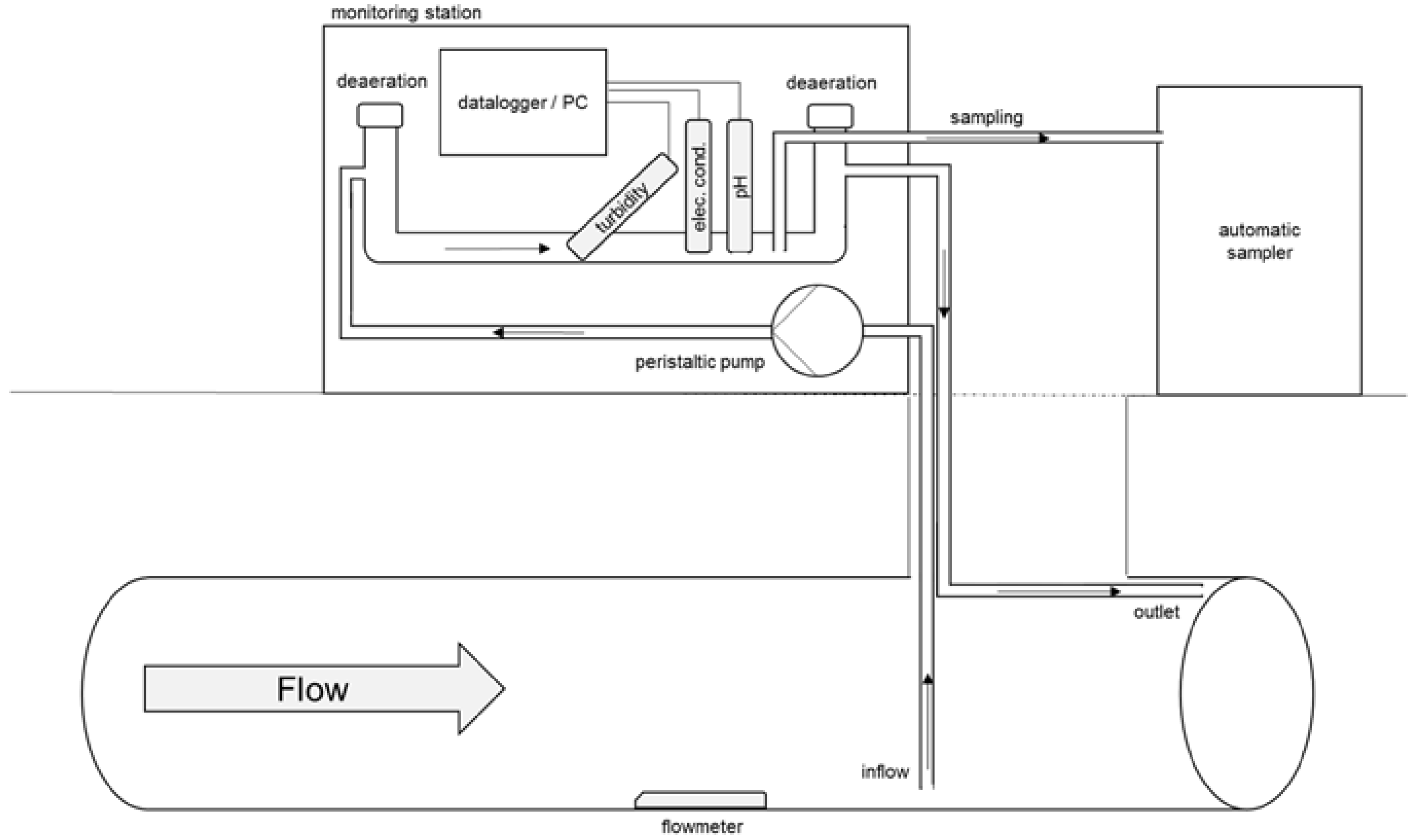
In contrast to FR, quality sensors at PL, RC, and HT are integrated in a horizontal measurement pipe (63 mm, PVC, length: 1.5 m) of an external monitoring station (
Figure 1). In case of an event stormwater is pumped to the measurement pipe by a peristaltic pump (Delasco 2Z3, PCM) through a hose (20 mm, PVC) whose orifice is fixed in the middle of the stormwater pipe 1.5 cm above the ground. The suction velocity in the hose is about 1.5 m/s with a corresponding flow of approx. 0.5 L/s. Stormwater flows with approx. 0.18 m/s through the measurement pipe and is later discharged to the sewer.
At these sites, the sampling program starts if the water level in the stormwater pipe exceeds 1.5 cm. Samples of all sites are tested for total suspended solid (TSS) concentrations based on a standard method given in [
8], and fine solids less than 63 µm (TSS63) according to the protocol given in [
9].
An online measurement data management system was applied to supervise all monitoring stations and to reduce data loss [
10].
2.3. Calculation of Continuous TSS Time Series
The turbidity of selected samples was measured to estimate the correlation to TSS. Initially, this has been conducted in the original sample bottle (PE, squared base, slightly transparent). Due to significant variance of the measured turbidity, a black cylindrical PE-HD bottle (diameter 10.8 cm, height 18.1 cm) has been used later. While measuring the turbidity, the sample is homogenized with a magnetic stirrer at 450 rpm. The five-minute mean of the turbidity is recorded. Calibration of turbidity probes was conducted with formazine primary standard solutions. TSS concentrations and the corresponding turbidity values were subjected to correlation analysis. The resulting linear regression equations are used to create continuous TSS time series from raw turbidity signals. Discussing the uncertainties through this conversion would exceed the scope of this paper and are therefore not presented here. The reader is referred to the literature [
11,
12,
13].
2.4. Data and Analysis
All sensor signals were logged with a 1 min interval. High-resolution online runoff and quality data is available for approx. 2.5 years (FR and RC), 1.5 years (PL), and 0.5 years (HT), respectively. Rainfall runoff events were statistically analyzed using rainfall, runoff, and pollutant characteristics. Events with a minimum rainfall depth of
H > 2 mm, maximum rainfall intensity in 60 min of Imax60 > 2.5 mm/h, and complete runoff/turbidity data are selected, only. Rainfall events below these criteria usually do not contribute to relevant runoff and are therefore excluded. Based on continuous runoff and TSS time series data, event volumes, event loads, and event mean concentrations are calculated according to Equations (1)–(3). Furthermore, event characteristics were subjected to correlation analysis with special emphasis to TSS loads.
where
i = index of time series,
n = number of data points of an event,
Qi = runoff at index
i,
Δt = time interval (i.e., 1 min), and
Ci = TSS concentration at index
i.
The intra-event distribution of TSS loads are examined by means of mass-volume-curves (
M (
V)-curves, [
14,
15]).
M (
V)-curves describe the proportion of transported mass at a given runoff volume proportion. This method is usually used to visualize transported mass proportions and to analyze the first-flush phenomenon. Knowledge of catchment-specific first-flush characteristics is crucial to designing cost-effective treatment or storage structures. However,
M (
V)-curves tend to be site-specific and vary greatly from event to event [
6]. Aggregation of similar
M (
V)-curves is therefore required to extract relevant information. [
16] for example, divide
M (
V)-curves in three different zones to classify similar events. Zone A contains curves with a dominant first-flush effect, while curves in Zone C tend to be more last-flush affected. Curves in Zone B are near the bisecting line and show a runoff-proportional mass transport.
In this paper,
M (
V)-curves are also used to characterize the two types of wash-off process, namely source-limited and transport-limited wash-off [
17,
18]. Source-limited runoff events have, in general, sufficient energy to wash off all available particles on the surface. This occurs if either masses on the surface are rather limited or the kinetic energy of rainfall/runoff is high enough. Transport-limited events are not able to completely remove available masses. Typically, these events occur either if the available masses are adequately high or the kinetic energy of runoff is insufficient.
M (V)-curves are calculated for the four study sites and compared. A seasonal differentiation is included. Instead of using zones, boxplots of the transported mass proportions are created at runoff volume quantiles to group M (V)-curves. With calculated and visualized interquartile ranges (IQR), the event variability and main wash-off trends can be observed and characterized.
3. Results
3.1. TSS Sample Statistics
Table 1 summarizes TSS sample statistics at the four study sites. Statistics were also calculated for the dataset excluding outliers. Due to non-normality of the dataset, outliers are conservatively considered and defined as points beyond the mean ± four times the standard deviation. Mean and standard deviation are iteratively computed while potential outliers are excluded.
At site
FR, 193 samples were analyzed from 40 events. With the 0.75 percentile being 14.2 mg/L, the flat roof clearly shows low TSS potential and distributions are similar to other findings [
19,
20,
21].
For site
RC, 269 samples of 39 events were taken. The distribution of TSS concentration also reveals low TSS contribution. Compared to the results of [
22], values are lower than TSS concentrations of a separated sewer system in Germany. The mean value of 114.3 mg/L and the standard deviation of 339 mg/L indicates high variation. However, these statistics are strongly influenced by the maximum value of 3645 mg/L. The 0.9 percentile being at 205 mg/L confirms this. 140 samples from 38 events were analyzed for site
PL. TSS concentration ranges from 7.3 mg/L to 1842 mg/L, with the median at 170 mg/L. At
HT, 92 samples of 17 events were collected. Compared to other studies at high-trafficked streets [
23], the TSS statistics are significantly lower. For example, the median of 77.4 mg/L is less than half as the median in their study (175 mg/L).
3.2. Relationship between TSS and Turbidity
To create continuous TSS data from online turbidity data, correlation functions are determined. Due to the change of bottle type in which the turbidity was measured, correlation functions were established with only a subset of all samples presented in
Table 2. The range of the sample subset is within the range of all samples with outliers being excluded. Only the maximum value at site RC is slightly higher (580.1 mg/L compared to 569.1 mg/L) and therefore still used for analysis. Both linear and non-linear relationships were tested. Since non-linear functions did not significantly outperform linear functions, only linear regression coefficients are listed in
Table 3. The goodness-of-fit of the linear regression is visually verified and numerically expressed by r-squared. With the lowest r-squared being at 0.68, all linear regression models show a good fit of the underlying dataset.
3.3. Event Database
An overview of the event database with continuous measurement data is given in
Table 4. It contains the number of total observed events and the number of events which are excluded from further analysis. Events are rejected if either selection criteria are violated or if measurement data is doubtful. In this respect, sites FR and RC show a high number of events with doubtful data. This is mainly caused by almost constantly low turbidity values (FNU < 15) in the course of an event. For site FR this can be justified with few particles in the runoff. At site RC, this is also caused by pumping difficulties. Gaps due to measurement failures of runoff and quality sensors are rarely present. Turbidity gaps are only observed if stormwater contained substances which caused intensive foaming in the measurement pipe. However, in total, 65 events were analyzed at FR, 23 at site RC, 46 at PL, and 16 at HT. Descriptive statistics of selected event characteristics are given in
Table 5.
3.4. Correlation Analysis
Table 6 shows Pearson correlation coefficients for TSS loads and selected variables at the four study sites. A strong correlation of rainfall intensities and mean/max runoff to TSS loads can be observed at site FR. This effect is also evident but less intense at sites PL and HT. However, the variable
Imean (mean rainfall intensity) has only a strong influence at FR (0.8). Rainfall depths seem to be strongly correlated to TSS loads at site HT, only. The overall rainfall duration does not correlate with TSS loads at any site. Correlation of the variables runoff volume (Vol) and antecedent dry weather periods (ADWP) to TSS loads can be noticed only at site HT and PL, respectively.
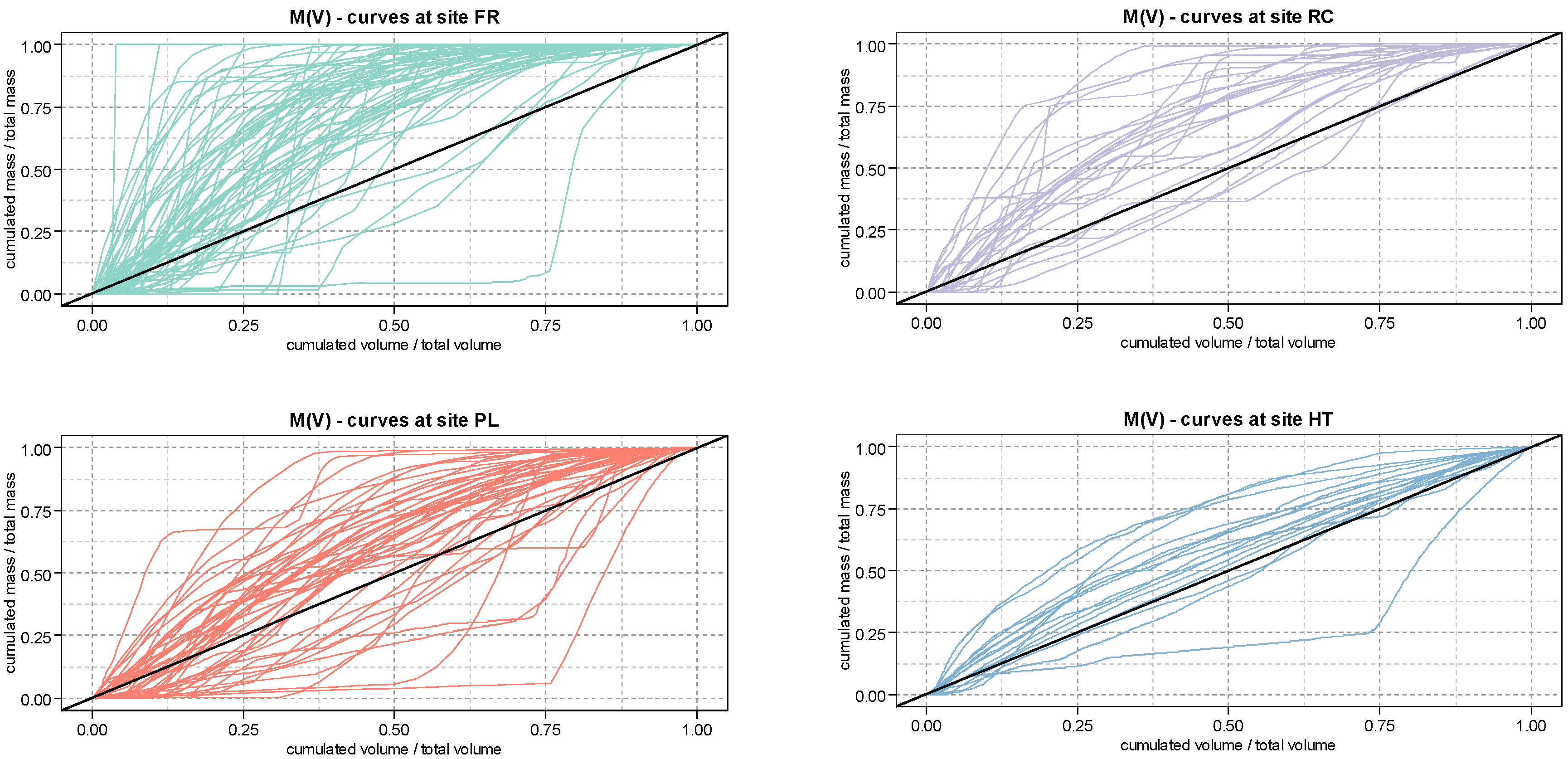
3.5. Intra-Event TSS Load Distributions
Intra-event distributions of TSS load are studied with site-specific
M (
V)-curves (
Figure 2). Clearly, all sites show large variability of intra-event TSS load distribution which confirms findings of other studies [
6,
7] also for microscale sites. However, from the four study sites it can be observed that the more curves are taken into account the variability increases. Therefore, boxplots at runoff volume quantiles are used to depict the main tendency of wash-off behavior. This enables a visual comparison between site and season-specific
M (
V)-curves.
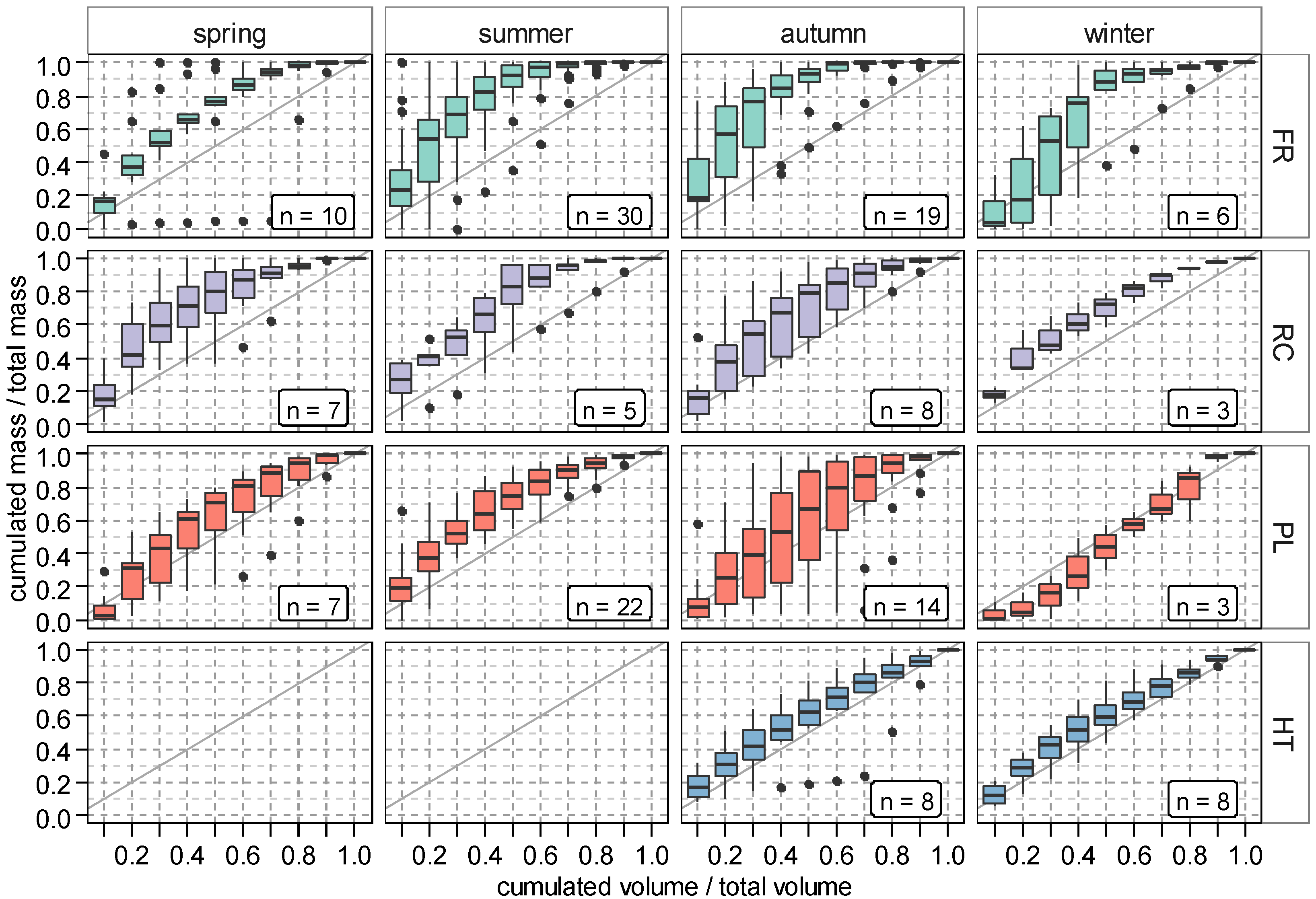
Figure 3 shows boxplots of
M (
V)-curve distributions at given runoff volume quantiles for each of the study sites. At site
FR, in most cases a large portion of pollution loads tend to be washed-off in the first period of an event. In addition, distances between the first and third quartile (interquartile range, IQR) increases until 20% of runoff volume and decreases afterwards. This generally indicates a decreasing event variability. In this respect, after 60% of runoff volume, most pollutants are already washed off. With regard to site
PL and
RC, the IQR rises until 20% of runoff volume and almost constantly continues up to 60% of runoff volume. At site
HT, the IQR is merely changing in the first 80% of runoff volume. Although, the number of events taken into account is likely to affect the interquartile ranges,
M (
V)-curves from site HT are noticeably closer to the bisecting line than
M (
V)-curves from site FR. Similarly,
M (
V)-curves from PL are closer to the bisecting line compared to the
M (
V)-curves from site RC.
3.6. Seasonal Intra-Event TSS Load Distribution
Figure 4 shows
M (
V)-curve distributions for different seasons. At FR, the
M (
V)-curves start steeper in spring, summer, and autumn periods, which indicates a more pronounced first flush. Contrarily, in winter, the
M (
V)-curves show a less dominant wash-off behavior at the beginning of the events. At site PL, the variability is highest during spring and autumn periods. Events during summer months show similar wash-off behavior, which is indicated by relatively low IQR. The three events in the winter are characterized by a delayed wash-off, but cannot be statistically interpreted due to small number of events.
M (
V)-curve distributions at site RC are comparable to PL with the highest variability during spring and autumn months. Pollutants tend to be washed-off in the first periods of an event. For site HT, monitored events are available in the autumn and winter months, only. Both seasons show comparable wash-off behavior, which is characterized by runoff almost proportional to washed-off loads, low IQR, and close distance to the bisecting line.
4. Discussion
From the correlation analysis it is stated, that firstly rainfall intensity (Imax5, Imax60) has a strong influence on TSS loads at small catchments with a high proportion of impervious surfaces (FR, PL, HT). Secondly, this effect decreases with increasing catchment size. Thirdly, in residential catchments which consist of multiple subcatchments (e.g., roofs, streets, parking lots) the correlation between rainfall event characteristics and TSS loads are strongly attenuated. The low correlation of the antecedent dry weather period suggests that this parameter is inappropriate to describe the pollutant build-up. However, in this study, the average antecedent dry weather period is about three days. This means pollutants are mostly accumulated shortly after an event and therefore exposed to other influential processes such as wind-driven processes.
Analysis of M (V)-curves suggests, that firstly, microscale sites show, in general, a more pronounced first-flush effect and only a few events with a delayed wash-off process. Secondly, the wash-off process at FR seems to be source limited because of the majority of particles are washed-off after 60% of runoff volume and the IQR is significantly low at the end of the events. Thirdly, in contrast, PL and HT show a more transport-limited wash-off because the IQR is closer to the bisecting line at the end of the events. Finally, it is assumed, that RC’s wash-off processes are influenced by a composition of subcatchments, such as roofs, streets, and parking lots, which is explained by the intermediate position of RC in comparison to FR, HT, and PL. In fact, runoff from different surfaces is superposed and therefore pollution transport processes are mixed.
From seasonal M (V)-curves it can be observed, firstly, that M (V)-curve distributions at FR show the largest variability in the first 50% of runoff volume throughout the seasons except for spring. The delayed wash-off process during winter months can be caused by a low pollutant potential on surfaces, coarser particles with high densities, or by events with low rain intensities. Secondly, variability of M (V)-curve distribution, in general, is largest during autumn, especially for sites FR, RC, and PL. It can be assumed that this is mainly caused by high variability of rainfall intensities in conjunction with varying pollutant masses available at the surface. It must also be noted, that only few events were monitored during the winter months, which must be taken into account for further statistical analysis.
5. Conclusions
A long-term monitoring campaign was conducted to analyze stormwater pollutant processes at microscale sites with online sensors. Rainfall runoff events were statistically analyzed and intra-event TSS load distributions were site- and season-specifically examined by means of M (V)-curves. The correlation analysis reveals a strong relationship between rainfall intensity and event loads for small catchments with a high proportion of impervious surfaces, but not for the larger residential catchment. Furthermore, grouping M (V)-curves with boxplots at runoff volume quantiles enables the comparison of wash-off behaviors of different catchments. In general, the wash-off process at site FR (flat roof) tends to be source-limited. In contrast, sites PL (parking lot) and HT (high-traffic) show a transport-limited behavior. A seasonal analysis of M (V)-curve distributions demonstrated the large variability, especially during autumn.
With these results, this paper clearly highlights the need for a spatially more detailed assessment of stormwater quality runoff. This can be drawn from the subcatchment-specific wash-off behavior. Consequently, it can be recommended to use different wash-off models for different catchment types to adequately address transport-limited and source-limited catchments.


