Bayesian Regression and Neuro-Fuzzy Methods Reliability Assessment for Estimating Streamflow

Abstract

Accurate and efficient estimation of streamflow in a watershed’s tributaries is prerequisite parameter for viable water resources management. This study couples process-driven and data-driven methods of streamflow forecasting as a more efficient and cost-effective approach to water resources planning and management. Two data-driven methods, Bayesian regression and adaptive neuro-fuzzy inference system (ANFIS), were tested separately as a faster alternative to a calibrated and validated Soil and Water Assessment Tool (SWAT) model to predict streamflow in the Saginaw River Watershed of Michigan. For the data-driven modeling process, four structures were assumed and tested: general, temporal, spatial, and spatiotemporal. Results showed that both Bayesian regression and ANFIS can replicate global (watershed) and local (subbasin) results similar to a calibrated SWAT model. At the global level, Bayesian regression and ANFIS model performance were satisfactory based on Nash-Sutcliffe efficiencies of 0.99 and 0.97, respectively. At the subbasin level, Bayesian regression and ANFIS models were satisfactory for 155 and 151 subbasins out of 155 subbasins, respectively. Overall, the most accurate method was a spatiotemporal Bayesian regression model that outperformed other models at global and local scales. However, all ANFIS models performed satisfactory at both scales.

1. Introduction

For any given time and location along a river, streamflow is derived from a combination of surface water, soil water, and groundwater, but ultimately originates from precipitation [1]. The rainfall-runoff process is complex and includes many interconnected elements (e.g., evapotranspiration, infiltration, subsurface flow, spatial and temporal rainfall variations, land-use, topography, and soil type) that often cannot be accurately measured in a large study area [2,3,4,5,6,7,8].

Streamflow forecasting is a critical component for many engineering applications and environmental management strategies, such as dam construction, reservoir design, hydro-power generation, irrigation, water resources allocation, flood control, environmental protection, ecosystem sustainability, and ecological integrity [9,10,11,12]. Short-term streamflow forecasting, such as hourly and daily, is important for flood prediction and protection, while long-term forecasting on monthly and annual scales is useful for water resources planning and management [13].

Streamflow forecasting techniques are divided into two categories: process-driven and data-driven methods [13,14]. Process-driven methods describe the physical processes that govern streamflow in watersheds based on an understanding of physical phenomena. Data-driven methods are black-boxes that forecast streamflow by mapping inputs (hydro-meteorological) to the output (streamflow) mathematically, without considering the physical processes within a watershed [13].

Although process-driven, physically-based methods can capture and predict the impacts of changes in landscape management practices on streamflow [15,16], they require intensive information on hydrogeology, soils, topography, etc., which are often difficult to obtain and measure [17]. Utilization of physically-based models are complex, time consuming, and require intensive calculations and expert knowledge [18], making their operation by watershed managers and stakeholders difficult [19]. Meanwhile, stakeholder involvement is crucial in developing a successful watershed management plan [20,21,22] and this cannot be achieved unless stakeholders and watershed managers are able to effectively use scientific tools for decision making [23]. These drawbacks demand more cost-effective techniques for streamflow calculation, especially for assessing the impacts of different management scenarios on streamflow, which requires extensive model simulation.

In recent years, new data-driven methods, such as soft computing, have become effective alternative techniques to physically-based models in water resources management. Soft computing techniques are cost effective methods that can be utilized for solving complex problems by approximation [24]. However, these methods fall short of capturing hydrological responses to significant changes in physiographical (e.g., land-use/land-cover) and climatological (e.g., climate change) characteristics of a watershed. Artificial neuro-fuzzy inference systems (ANFIS) and Bayesian regression methods have received more attention in recent years in the water resources field due to their ability to model sophisticated non-linear systems such as streamflow and contaminant transport [25,26,27,28,29,30,31,32,33].

In this study we used a physically-based hydrological model, the Soil and Water Assessment Tool (SWAT), to simulate streamflow in a large and diverse watershed. We trained and tested two data-driven methods (ANFIS and Bayesian regression) to evaluate their capability in estimating streamflow both at the watershed outlet and at each subbasin outlet, as compared to the SWAT model. The application of data-driven methods will significantly reduce the computational time and effort required for examining future management scenarios while being simple enough to be used by stakeholders and watershed managers for decision making. They will save considerable time and resources usually spent on data collection and streamflow estimation because data-driven methods require fewer input parameters than physically-based models.

2. Materials and Methods

2.1. Study Area

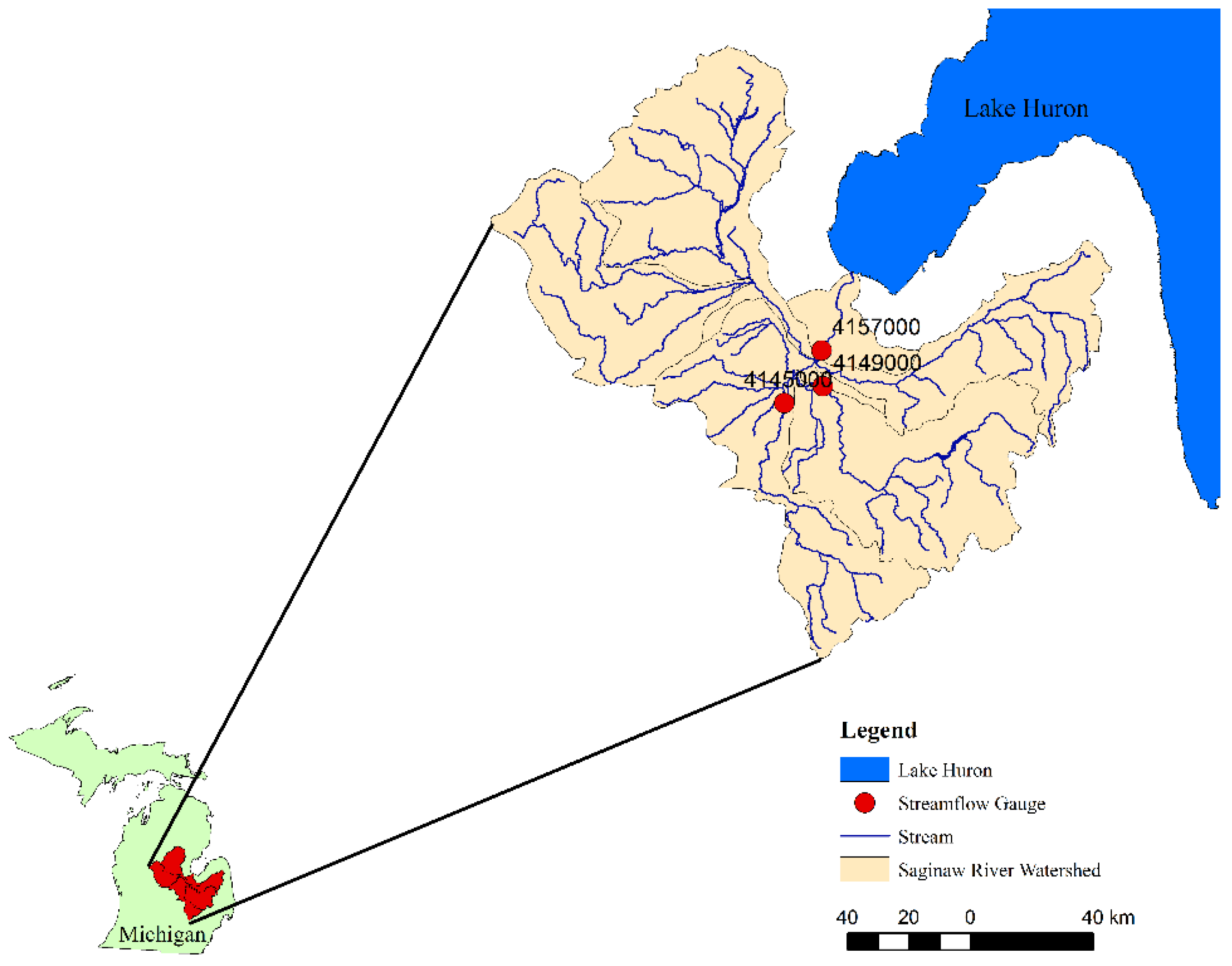
The Saginaw River Watershed (hydrologic unit code-HUC 040802) located in Michigan’s Lower Peninsula (Figure 1), was selected for this study. This is the largest watershed in Michigan and consists of six eight-digit HUCs; the Tittabawassee (04080201), Pine (04080202), Shiawassee (04080203), Flint (04080204), Cass (04080205), and Saginaw (04080206). The watershed drains about 15% of Michigan’s land area into Lake Huron. The total watershed area is 22,260 km², of which 45% is forest, 38% is agriculture and pasture, 11% water and wetlands, and the remaining is urban area. The average watershed elevation is 242 m above mean sea level.

2.2. Modeling Procedures

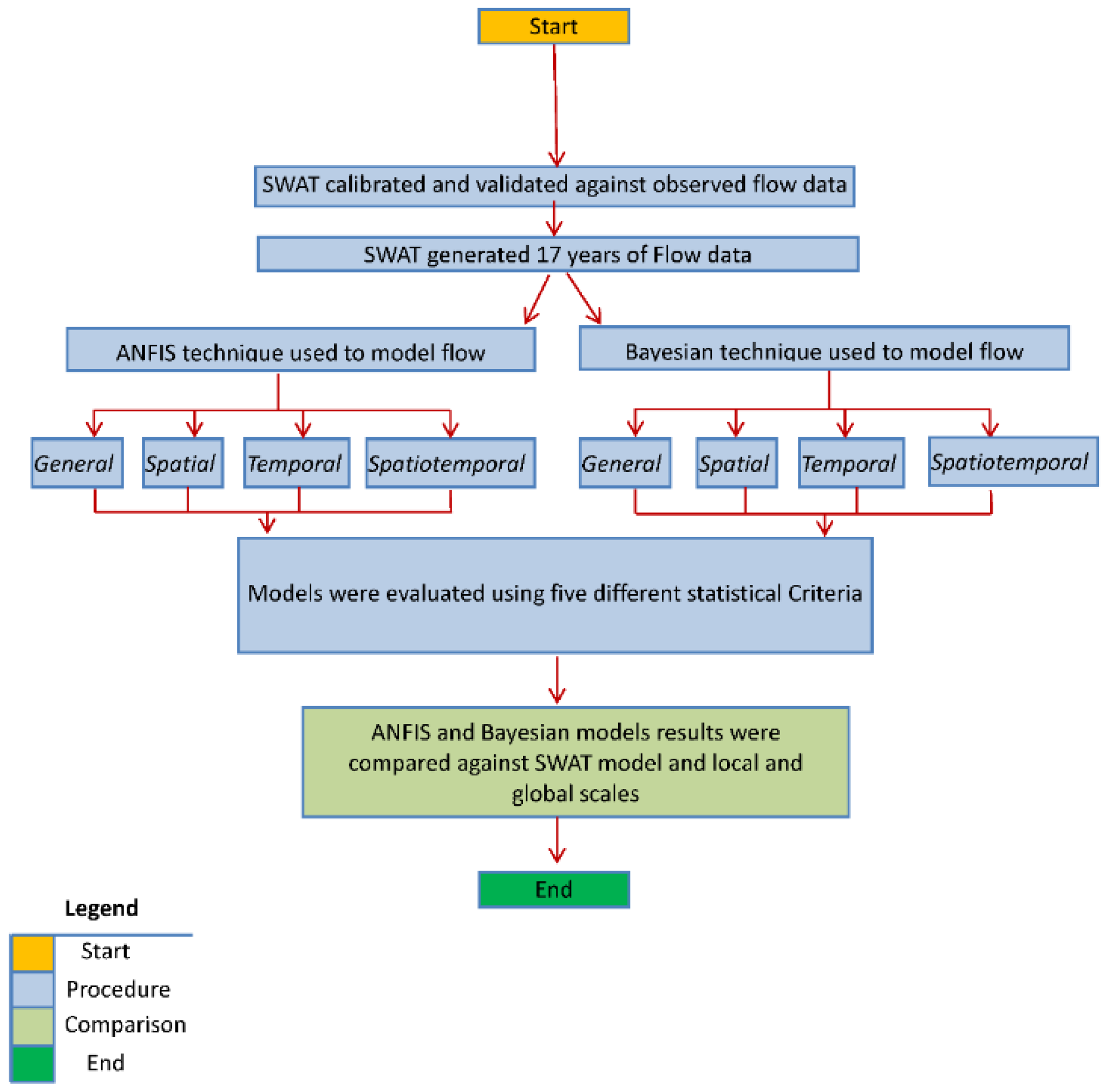
A multi-step modeling process was used to simulate streamflow within the Saginaw River watershed (Figure 2). The process began with setup and calibration of the physically-based SWAT model. The model was run for 17 years to calculate annual average flow rate for 155 streams within the study area. The ANFIS and Bayesian regression techniques used unique sets of watershed parameters and SWAT model outputs to investigate streamflow predictions based on four model structures: general, spatial, temporal, and spatiotemporal. The results of these models were evaluated against streamflow data obtained from the calibrated SWAT model using five statistical criteria. These criteria were used to select the best data-driven method and model structure that can accurately predict streamflow data.

2.3. Physically-Based Hydrological Model Setup

SWAT was used to simulate long-term daily streamflow in the Saginaw River watershed. SWAT was developed by the United States Department of Agriculture–Agricultural Research Service (USDA–ARS) to simulate flow and pollution transport [34]. SWAT is one of the most widely used spatially-explicit watershed models in the world [35]. The model simulates flow, sediment, nutrient, and pesticide transport, crop growth, and management practices, providing insight for decision makers and watershed managers [36]. In SWAT, basic computational units are known as hydrologic response units (HRUs), which are areas of homogeneous land-use, soil, and slope. Overland flow and pollutants in HRUs are aggregated to the subbasin level and routed through the river network.

Many datasets are required for setting up the SWAT and data-driven models, including soils, climate, land-use, and topography. Soil physical and chemical characteristics were obtained from the State Soil Geographic Database [37] at a 1:250,000 resolution. Land-use information, including crop-specific classifications, was obtained from the 2008 Cropland Data Layer (56 m resolution) developed by the USDA National Agricultural Statistics Service [38]. Topographic data was acquired in the form of a 90 m resolution digital elevation model (DEM) from the Better Assessment Science Integrating Point and Nonpoint Sources (BASINS version 4.1, United States Environmental Protection Agency: National Exposure Research Laboratory, Research Triangle Park, NC, USA) program [39]. Stream network data was obtained from the United States Geological Survey (USGS) National Hydrography Dataset (NHD) [40]. Based on the NHD and DEM data, the watershed was delineated into 155 subbasins. Climate data was obtained from the National Climatic Data Center (NCDC) with 19 years (1990–2008) of observed daily temperature and precipitation for 15 temperature stations and 19 precipitation stations. Meteorological data, such as solar radiation, wind speed, and relative humidity, were simulated using the SWAT built-in weather generator. The SWAT model included locally relevant agricultural management operations and rotations from Love and Nejadhashemi [41].

Observed daily streamflow data for the period of 2002–2007 was obtained from USGS gauging stations 04145000, 04149000, and 04157000 (Figure 1). The SWAT model was calibrated from 2002 to 2004 and validated from 2005 to 2007 on a daily time-step. Next, the calibrated SWAT model was run for 19 years (1990–2008), using the first two years for model warm-up, with the remaining 17 years representing the model simulation period. For the 155 subbasins, a total of 2635 annual streamflow data points were obtained for the watershed.

2.4. Data-Driven Hydrological Models Setup

The study watershed only contained observed streamflow data at four of 155 subbasins. Therefore, the calibrated SWAT model outputs were used to judge the predictive data-driven models’ capability in estimating flow at local and global scales. SWAT can estimate streamflow beyond the four gauging stations for all stream segments in the watershed. This information was used to develop two data-driven methods, ANFIS and Bayesian regression. Thirteen predictor variables were obtained from SWAT model outputs, including time period, geographical coordinates, precipitation data, the total upstream drainage area, four different land-uses (urban, forest, agriculture, and water), and four hydrologic soil groups (A, B, C, and D) to model daily average flow rate. The land-use and soil group variables were calculated as percentage of the total upstream area.

To investigate the effect of different spatial and temporal watershed parameters on streamflow predictions, general, spatial, temporal, and spatiotemporal model structures were considered. For the general model structure hydro-meteorological and watershed characteristics were considered without any spatial or temporal effects. For the spatial model structure, geographical coordinates were added (without time effects) to the set of predictor variables of the general model. For the temporal model structure, time period (without spatial effects) was added to the hydro-meteorological and watershed characteristics. For the spatiotemporal model structure, geographic coordinates and time period were added to the hydro-meteorological and watershed characteristics variables.

2.5. ANFIS

ANFIS is a hybrid model of artificial neural networks (ANN) and Sugeno fuzzy logic inference systems. This method uses the ANN learning ability for the fuzzy inference system to more efficiently compute fuzzy rules and implement three fuzzy control steps (fuzzification, inference, and defuzzification) [42]. The MATLAB (version 7.12.0, MathWorks, Natick, MA, USA) fuzzy logic toolbox was used to perform ANFIS analysis. MATLAB’s “genfis2” function (which uses subtractive clustering to produce partitions for the data) was used to create fuzzy membership functions (MFs). The number of data subsets depends on the cluster radius value (a small radius results in more clusters and rules and vice versa). Gaussian MFs were used for all input variables and linear parameters were selected for the output MFs. To select the best model structure, ten-fold cross-validation was employed. Here, 90% of the data was used to build the model (the training dataset) and checked on the remaining 10% (the testing dataset). In this way, ten models were generated for all of the ten-folds of data. The average performance (smallest average root-mean-square error—RMSE) of the ten test sets was the criteria for selecting the best structure.

After selecting the most appropriate model structure (general, spatial, temporal, and spatiotemporal), the best model was selected from the ten generated models. Each model was tested against all of the ten test sets, and the lowest average error for all test sets was the criteria for selecting the best model [32].

Variable Selection for ANFIS

The ANFIS modeling process started with selecting best set of predictor variables for each model structure. Afterward, the best model was used for flow prediction at global (watershed outlet) and local (individual subbasin) scales.

Cobaner [43] and Sanikhani Kisi [44] concluded that using a large number of input variables in fuzzy logic models significantly increases the noise in model prediction due to a substantial increase in the number of rules. Due to this limitation, a set of seven input variables were used. All possible variable combinations were explored for each model structure. Accordingly, predictor variables for the ANFIS general (non-random) model structures included upstream drainage area, precipitation, three types of land-use and two soil types. This technique leads to 20 possible variable combinations that were used to select the best variable set describing flow rate in the watershed. For the spatial model structure, total upstream area, precipitation, latitude, longitude, two types of land-use and one type of soil type were used, which resulted in 24 possible variable combinations. For the temporal model structure, upstream area, precipitation, time period (year), three types of land-use and one soil type were used, resulting in 16 possible variable combinations. For the spatiotemporal model structure, upstream total area, precipitation, latitude, longitude, time period, one type of land-use and one soil type were used, which resulted in 16 possible variable combinations.

2.6. Bayesian Regression Method

The Bayesian regression models were developed in MATLAB (version 7.12.0) [45]. The four model structures were also used for the Bayesian regression method. For each model structure, a set of ten input variables (covariates) were used for the modeling process. The two variables of water from land-use and type-D from soil group were excluded from the variables to remove singularity of the design matrix (because the sum of the all land-uses and soil groups are equal to one) and because an intercept in the Bayesian regression model is included. Precipitation, total upstream area, urban land-use, forest land-use, agricultural land-use, type-A soil, type-B soil, and type-C soil variables were used in addition to a neighborhood matrix and a year-specific random effect. The selected covariates were standardized for the modeling process. The general model structure was created without any temporal and spatial random effects. For the temporal model structure only temporal random effects were included in the general model structure. For the spatial model structure only spatial random effects were included in the general model. Finally, for the spatiotemporal model structure both temporal and spatial random effects were included in the general model.

2.6.1. Bayesian Regression Model Specification

For a data containing response Y_st observed for s = 1, 2, · · ·, N geographic regions and t = 1, 2, · · ·, T years. The following multiplicative spatiotemporal model is presented in Equation (1).

$$Y_{\text{st}}={\displaystyle \sum _{j=1}^p{X}_{stj}{\mathsf{\beta }}_j}+u_{st}+{\mathsf{\epsilon }}_{st}$$

(1)

In Equation (1), j indexes the p-covariates, which includes the intercept. The regression coefficient β_j for the jth predictor X_stj measures its effect on the response variable. u_st is the multiplicative spatiotemporal random effect that captures the variability due to the spatial and temporal effects. ε_st is the residual. We assume ${\mathsf{\epsilon }}_{st} ~ N(0,{\mathsf{\delta }}^2)$ to measure the nugget effects and u the multiplicative spatiotemporal random effect follows the distribution as following in Equation (2):

$$\mathit{u} ~ N(0,{\mathsf{\tau }}^2\mathit{A}(\varphi )\otimes \mathit{D}(\mathsf{\gamma }))$$

(2)

which assumes separable spatiotemporal dependence, i.e., the spatial correlation matrix A(φ) and the temporal correlation matrix D(γ) are separately generated by two underlying Gaussian processes, that are both assumed to be Markovian, such as conditional autoregressive (CAR) structure for the spatial dependence, and autoregressive (AR) with order 1 for the temporal dependence. The $\otimes$ operator indicates the Kronecker product of two matrices. The assumption is made for simplicity and computational efficiency as both correlation matrices have closed inverse form for likelihood calculation. The model in Equation 1 assumes a single NT × 1 spatiotemporal random effect that allows the interactions of the spatiotemporal dependences with a single τ² to measure its variation. The model can be again written in the canonical form of a mixed-effects model in Equation (3).

$$\mathit{Y} ~ N(X\mathsf{\beta }+Zu,{\mathsf{\delta }}^2{\mathit{I}}_{NT})$$

(3)

For a Gibbs sampler, the full conditional distributions of fixed-effects and random-effects are as shown in Equations (4) and (5) [46].

$$\begin{array}{l}\mathsf{\pi }(\mathsf{\beta }|\mathrm{...})=N({\mu }_{\mathsf{\beta }},{\mathrm{\Sigma }}_{\mathsf{\beta }})\{\begin{array}{l}{\mathrm{\Sigma }}_{\mathsf{\beta }}={\mathsf{\delta }}^2{({\mathit{X}}^{\text{'}}\mathit{X})}^{-1}\\ {\mathsf{\mu }}_{\mathsf{\beta }}={({\mathit{X}}^{\text{'}}\mathit{X})}^{-1}{\mathit{X}}^{\text{'}}(\mathit{Y}-{\mathit{Z}}_u\mathit{u}-{\mathit{Z}}_{v}v)\end{array}\end{array}$$

(4)

$$\begin{array}{l}\mathsf{\pi }(\mathit{u}|\mathrm{...})=N({\mathsf{\mu }}_u,{\mathrm{\Sigma }}_u)\{\begin{array}{l}{\mathrm{\Sigma }}_u={({\mathsf{\delta }}^{-2}{I}_N+{\mathsf{\tau }}^{-2}A{(\varphi )}^{-1}\otimes D{(\mathsf{\gamma })}^{-1})}^{-1}\\ {\mathsf{\mu }}_u={\mathrm{\Sigma }}_u{\mathit{Z}}^{\text{'}}(\mathit{Y}-X\mathsf{\beta })/{\mathsf{\delta }}^2\end{array}\end{array}$$

(5)

The conditional distributions of variance components and spatiotemporal dependence are presented in Equations (6)–(10).

$$\mathsf{\pi }({\mathsf{\delta }}^2|\mathrm{...})=igamma(a_{\mathsf{\delta }}+NT/2,b_{\mathsf{\delta }}+{\mathsf{\epsilon }}^{\text{'}}\mathsf{\epsilon }/2)$$

(6)

$$\text{where }\mathsf{\epsilon }=\mathit{Y}-\mathit{X}\mathsf{\beta }-Zu$$

(7)

$$\mathsf{\pi }({\mathsf{\tau }}^2|\mathrm{...})=igamma(a_{\mathsf{\tau }}+NT/2,b_{\mathsf{\tau }}+{\mathit{u}}^{\text{'}}(\mathit{A}{(\varphi )}^{-1}\otimes \mathit{D}{(\mathsf{\gamma })}^{-1})\mathit{u}/2)$$

(8)

$$\mathsf{\pi }(\mathsf{\gamma }|\mathrm{...})\propto {|\mathit{D}(\mathsf{\gamma })|}^{-T/2}\exp \{\mathsf{\gamma }{\mathit{u}}^{\text{'}}(\mathit{A}{(\varphi )}^{-1}\otimes W)u/(2{\mathsf{\tau }}^2)\}.\mathit{I}(\mathsf{\gamma }\in ({\mathsf{\lambda }}_N^{-1},{\mathsf{\lambda }}_1^{-1}))$$

(9)

$$\mathsf{\pi }(\mathsf{\phi }|\mathrm{...})\propto {|\mathit{A}(\mathsf{\phi })|}^{-N/2}\exp \{-{\mathit{u}}^{\text{'}}(\mathit{A}{(\mathsf{\phi })}^{-1}\otimes D{(\mathsf{\gamma })}^{-1})u/(2{\mathsf{\tau }}^2)\}.\mathit{I}(\mathsf{\phi }\in (-1,1))$$

(10)

2.6.2. Bayesian Regression Models Comparisons

The proposed model structure can be implemented with only spatial components, only temporal components, or with both spatiotemporal components masked to evaluate the significance of each component. To compare the Bayesian regression models, the deviance information criterion (DIC) for the mixed-effects model is used. The DIC₄ based on complete likelihood [47] is presented in Equation (11).

$$\begin{array}{ll}{\text{DIC}}_4& =-4{\mathit{E}}_{\mathsf{\theta },\alpha }[\log f(\mathit{Y},\mathit{\alpha }|\mathsf{\theta })|\mathit{Y}]+2{\mathit{E}}_{\alpha }[\log f(\mathit{Y},\mathit{\alpha }|{\mathit{E}}_{\mathsf{\theta }}[\mathsf{\theta }|\mathit{Y},\mathit{\alpha }])|\mathit{Y}]\hfill \\ & \stackrel{\mathsf{\Delta }}{=}-4{\mathit{E}}_1+2{\mathit{E}}_2\hfill \end{array}$$

(11)

where ${\mathit{E}}_{\mathsf{\theta }}[\mathsf{\theta }|\mathit{Y},\mathit{\alpha }]$ can be evaluated by sampling θ for each posterior sample of the random effects α and the obtained mean. $\overline{D(\mathsf{\theta })}=-2{\mathit{E}}_1$ is the posterior expected value of the joint deviance, and $p_{D4}=\overline{D(\mathsf{\theta })}+2{\mathit{E}}_2$ is the measure of model dimensionality. Therefore, a smaller $p_{D4}$ indicates a simpler model. A smaller DIC4 indicates better predictive power. For the multiplicative model (Equation (1)) the random effect α = u.

To assess the model fit given the L posterior samples of parameters ${({\mathsf{\beta }}_j^{(l)},u_s^{(l)},v_t^{(l)})}_{l=1,2,\mathrm{...},L}$, the fitted value ${\widehat{Y}}_{st}$ can be calculated in Equation (12).

$${\widehat{Y}}_{st}=\frac{1}{L}\sum _{l=1}^L(\sum _{j=1}^p{X}_{stj}{\mathsf{\beta }}_j^{(l)}+u_s^{(l)}+v_t^{(l)})=\sum _{j=1}^p{X}_{stj}{\hat{\mathsf{\beta }}}_j+{\hat{u}}_s+{\hat{v}}_t$$

(12)

where, ${\hat{\mathsf{\beta }}}_j,{\widehat{u}}_s$ and ${\widehat{v}}_t$ are posterior mean estimates.

2.7. Methods Evaluation Criteria

To compare performance of the Bayesian regression and ANFIS models, five different evaluation criteria were used: coefficient of determination (R²), RMSE, ratio of the root mean square error to the standard deviation of measured data (RSR), Nash-Sutcliffe efficiency coefficient (NSE), and percent bias (PBIAS).

The coefficient of determination is the squared Pearson product moment correlation coefficient, which shows the degree that two variables are related. It ranges between zero and one, where 1 indicates perfect correlation [48].

$$R^2={{\displaystyle \left[\frac{{\mathrm{\Sigma }}_{s=1}^N{\mathrm{\Sigma }}_{t=1}^T(Y_{st}-\overline{Y})({\widehat{Y}}_{st}-\widehat{\overline{Y}})}{\sqrt{{\mathrm{\Sigma }}_{s=1}^N{\mathrm{\Sigma }}_{t=1}^T{(Y_{st}-\overline{Y})}^2{({\widehat{Y}}_{st}-\widehat{\overline{Y}})}^2}}\right]}}^2$$

(13)

where, Y_st and ${\widehat{Y}}_{st}$ are observed and predicted values for s-th subbasin and t-th year, respectively, with N representing the total number of subbasins and T representing study period. $\overline{Y}$ and $\widehat{\overline{Y}}$ are averages of observed and predicted values for s-th subbasin and t-th year, respectively. R² > 0.5 represents satisfactory model performance [15].

An RMSE of 0 is the best prediction of the observed values [48,49].

$$RMSE=\sqrt{\frac{{\mathrm{\Sigma }}_{s=1}^N{\mathrm{\Sigma }}_{t=1}^T{(Y_{st}-{\widehat{Y}}_{st})}^2}{NT}}$$

(14)

RSR is the standardized RMSE using the observations’ standard deviation. RSR of zero indicates perfect prediction, while RSR > 0.7 represents unsatisfactory model performance [49].

$$RSR=\frac{RMSE}{\mathsf{\sigma }}=\frac{\sqrt{{\mathrm{\Sigma }}_{s=1}^N{\mathrm{\Sigma }}_{t=1}^T{(Y_{st}-{\widehat{Y}}_{st})}^2}}{\sqrt{{\mathrm{\Sigma }}_{s=1}^N{\mathrm{\Sigma }}_{t=1}^T{(Y_{st}-\overline{Y})}^2}}$$

(15)

where, σ is the standard deviation of the observed values.

NSE is the relative magnitude of the residual variance compared to the measured data variance, where NSE equal to 1 is the best prediction [50].

$$NSE=1-\frac{{\mathrm{\Sigma }}_{s=1}^N{\mathrm{\Sigma }}_{t=1}^T{(Y_{st}-{\widehat{Y}}_{st})}^2}{{\mathrm{\Sigma }}_{s=1}^N{\mathrm{\Sigma }}_{t=1}^T{(Y_{st}-\overline{Y})}^2}$$

(16)

PBIAS measures the average tendency of the predicted data to be larger or smaller than their corresponding observed values, where an optimal PBIAS is equal to zero [50].

$$PBIAS=\frac{{\mathrm{\Sigma }}_{s=1}^N{\mathrm{\Sigma }}_{t=1}^T(Y_{st}-{\widehat{Y}}_{st})\times 100}{{\mathrm{\Sigma }}_{s=1}^N{\mathrm{\Sigma }}_{t=1}^T{Y}_{st}}$$

(17)

3. Results and Discussion

3.1. SWAT Model

The SWAT model was calibrated for three years (2002–2004), and validated for the following three years (2005–2007) based on daily stream flow data from three gauging stations. The model performed satisfactorily (

Table 1. Saginaw River Watershed calibration and validation results.

Station ID	Constituent	Statistic	Calibration	Validation	Overall
04145000	Flow	R2	0.81	0.76	0.79
		RMSE	8.21	9.58	8.92
		NSE	0.63	0.55	0.59
		PBIAS	5.38	3.51	4.30
		RSR	0.61	0.67	0.64
04149000	Flow	R2	0.77	0.73	0.75
		RMSE	17.42	17.38	17.40
		NSE	0.57	0.53	0.55
		PBIAS	26.62	−0.96	11.28
		RSR	0.66	0.68	0.67
04157000	Flow	R2	0.86	0.83	0.84
		RMSE	75.62	76.55	74.69
		NSE	0.69	0.66	0.67
		PBIAS	28.85	16.62	22.07
		RSR	0.56	0.58	0.57

), according to criteria established by Moriasi et al. [50] for NSE, PBIAS, and RSR.

3.2. ANFIS Method Performance

Considering the number of variables was constrained to seven in ANFIS, for each of the model structures different variable combinations were arranged from the available 13 predictors to select the best model structure (

Table 2. The parameter estimations and model assessment for the adaptive neuro-fuzzy inference system (ANFIS) method.

Parameter	Unit	Min	Mean	Max	General	Spatial	Temporal	Spatiotemporal
Time	Year	1992	–	2008	–	–	*	*
Latitude	Degree	42.7	43.4	44.2	–	*	–	*
Longitude	Degree	−85.2	−84.0	−82.9	–	*	–	*
Precipitation	mm	507	812	1132	*	*	*	*
Area	km2	76.2	1367.7	14,934.7	*	*	*	*
Agriculture	%	0.0	35.8	100.0	*	*	*	*
Urban	%	0.0	2.4	100.0	–	–	*	–
Forest	%	0.0	51.8	100.0	*	*	*	–
Water	%	0.0	10.0	100.0	*	–	–	–
A Soil	%	0.0	26.7	100.0	*	–	–	–
B Soil	%	0.0	56.6	100.0	*	–	*	*
C Soil	%	0.0	15.5	100.0	–	*	–	–
D Soil	%	0.0	1.2	39.3	–	–	–	–

Note: * Parameter was used for the model development.

). Total upstream area, precipitation, and agricultural land-use were the only variables that were selected by all model structures, which demonstrates their importance. Meanwhile, D-soil, water land-use, and A-Soil were the least important.

The calibration and validation results for each model structure are shown in

Table 3. ANFIS best-set calibration and validation average results.

Method Type	Calibration					Validation
	R2	RMSE	RSR	NSE	PBIAS (%)	R2	RMSE	RSR	NSE	PBIAS (%)
General	0.96	4.226	0.192	0.96	0.003	0.95	4.321	0.220	0.95	−0.375
Spatial	0.98	3.351	0.152	0.98	−0.002	0.96	3.654	0.196	0.96	−0.304
Temporal	0.93	8.149	0.263	0.93	−0.198	0.87	9.963	0.367	0.86	−0.656
Spatiotemporal	0.96	4.557	0.199	0.96	0.114	0.93	7.392	0.270	0.93	−0.268

. The spatial model structure is the best for flow prediction with NSE of 0.98 for calibration and 0.96 for validation. After selecting spatial model structure, the model was used for global and local predictions.

3.3. Bayesian Regression Method Performance

Spatiotemporal multiplicative random-effect models were considered for the Bayesian regression method. The eight selected covariates (inputs) were standardized using the neighborhood matrix and year-specific random effect. Depending on the model-specific assumptions for each model structure, the flow rates were estimated for each model structure (general, spatial, temporal, and spatiotemporal).

For the full spatiotemporal model, the convergence was well-committed for the first 15,000 iterations, and the last 1000 samples for each chain were used as the posterior distribution. We also fit the spatial version of the model in Equation (2) by fixing φ = 0, temporal version by fixing γ = 0, and non-random effects model (general) by ruling out u, which reduced the models to ordinary regressions. The parameter estimations and model assessment are summarized in

Table 4. The parameter estimations and model assessment for the Bayesian regression technique.

Parameter	General	Spatial	Temporal	Spatiotemporal
Intercept	0.90 (0.87, 0.94)	0.94 (0.88, 0.99)	0.92 (0.85, 1.04)	0.96 (0.78, 1.28)
Area	0.94 (0.90, 0.98)	1.03 (0.98, 1.07)	0.96 (0.88, 1.03)	1.11 (1.03, 1.22)
Urban	0.09 (0.04, 0.15)	0.08 (0.02, 0.13)	0.04 (−0.09, 0.17)	0.02 (−0.11, 0.11)
Forest	0.23 (0.16, 0.30)	0.27 (0.20, 0.34)	0.25 (0.08, 0.39)	0.29 (0.18, 0.36)
Agriculture	0.03 (−0.05, 0.12)	0.08 (−0.00, 0.17)	0.02 (−0.18, 0.21)	0.17 (0.04, 0.29)
A-soil	−0.25 (−0.53, 0.02)	−0.39 (−0.71, 0.09)	−0.50 (−1.32, 0.22)	−0.89 (−1.83, −0.23)
B-soil	0.26 (−0.03, 0.55)	0.13 (−0.20, 0.44)	0.05 (−0.81, 0.77)	−0.23 (−1.17, 0.42)
C-soil	0.26 (0.04, 0.47)	0.12 (−0.12, 0.36)	0.15 (−0.50, 0.66)	−0.21 (−0.84, 0.26)
Precipitation	0.24 (0.21, 0.28)	0.22 (0.17, 0.28)	0.21 (0.20, 0.22)	0.14 (0.12, 0.15)
Residual δ2	0.93 (0.88, 0.99)	0.58 (0.48, 0.67)	0.04 (0.03, 0.04)	0.01 (0.01, 0.01)
τ2	0.00	1.25 (0.85, 1.71)	0.38 (0.34, 0.42)	1.51 (1.36, 1.67)
Temporal ø	0.00	0.00	0.96 (0.95, 0.97)	0.97 (0.96, 0.97)
Spatial γ	0.00	0.85 (0.77, 0.91)	0.00	0.99 (0.98, 0.99)
$\overline{D(\mathsf{\theta })}$	7253.11	10,067.63	−2735.59	−6920.97
pD4	9.77	11.63	11.00	9.56
DIC4	7262.88	10,079.26	−2724.59	−9611.41

. We report the posterior mean estimates along with the lower and upper bounds of the 95% credible intervals in brackets. For the regression coefficients and dependence parameters, a 95% credible interval that does not span zero indicates statistical significance. Note the term “spatial” and “temporal” refer to the correlation only, because u is a spatiotemporal random effect with a single variation parameter ${\mathsf{\tau }}^2$ that measures its variation from spatial and temporal aspects. Therefore “temporal” does not mean no spatial effect is considered, but means that no spatial correlation is considered.

The lowest DIC₄ is the criterion for selecting the best prediction of mixed effect models (fixed and random effects). The results show that the spatiotemporal model fits the data perfectly, considering that both spatial and temporal correlations are highly significant, which further demonstrates the necessity of modeling the spatiotemporal dependencies.

In Table 4 the lowest DIC₄ is for the spatiotemporal model structure, indicating it was the best model structure for predicting the flow rate. The Bayesian regression temporal model structure performed the second best, while the performances of the two other model structures (general and spatial) were not promising due to their high DIC₄ values.

3.4. Global Application of ANFIS and Bayesian Regression Best Models at Watershed Scale

Table 5. ANFIS global estimations for each model structure using best estimation model.

Method Type	R2	RMSE	RSR	NSE	PBIAS
General	0.96	4.356	0.210	0.96	1.106
Spatial	0.97	3.550	0.172	0.97	1.574
Temporal	0.85	9.148	0.442	0.80	−3.437
Spatiotemporal	0.91	6.647	0.321	0.90	−1.464

and

Table 6. Bayesian regression global estimations for each model structure using best estimation model.

Method Type	R2	RMSE	RSR	NSE	PBIAS
General	0.66	170.820	8.254	−67.15	−248.367
Spatial	0.61	71.171	3.439	−10.83	−76.977
Temporal	0.98	2.696	0.130	0.98	0.306
Spatiotemporal	0.99	0.775	0.037	0.99	−0.057

show all model structures’ global predictions for ANFIS and Bayesian regression, respectively. All ANFIS model structures performed satisfactorily. The ANFIS spatial model structure was the best predictor of flow with the highest R² and NSE of 0.97 and lowest RMSE of 3.55, which according to model performance criteria, is very good [50]. Both the Bayesian regression spatiotemporal and temporal model structures performed better than the ANFIS spatial model structure with higher R² and NSE. The best prediction with Bayesian regression was for the spatiotemporal model structure with R² and NSE of 0.99, followed by the temporal model structure with R² and NSE of 0.98, while the results from the general and the spatial model structures were unsatisfactory (Table 6).

Figure 3 shows the performance of the best ANFIS model structure (spatial) versus the calibrated SWAT model flow rate results at the watershed outlet. Figure 4 shows the predicted flow for the Bayesian regression best model structure (spatiotemporal) versus the SWAT flow rate. The Bayesian regression spatiotemporal model structure predicted the flow rate almost perfectly, with few deviations from the line of best fit (the 45-degree line). Meanwhile, the ANFIS spatial model structure produced acceptable results.

3.5. Local Applications of ANFIS and Bayesian Regression Best Model Structures at the Subbasin Scale

To further test the performance of the model structures at the local scale, the ANFIS and Bayesian regression models were tested to estimate flow for all subbasin reaches within the study area. At the local scale, the data has two dimensions (spatial and temporal). For each subbasin there are only 17 data points, one for each simulation year.

Table 7. Performances of all model structures for both ANFIS and Bayesian regression methods at local scale (subbasin).

Model Structure	Technique	Subbasins with NSE ≥ 0.5
General model	ANFIS	149
	Bayesian Regression	56
Spatial model	ANFIS	151
	Bayesian Regression	107
Temporal model	ANFIS	117
	Bayesian Regression	155
Spatiotemporal model	ANFIS	138
	Bayesian Regression	155

shows the results of both methods’ best global model structures at the subbasin level. The best performance occurred for the Bayesian regression spatiotemporal and temporal model structures, which were satisfactory for all the 155 subbasins according to Moriasi et al. [50] criteria. The ANFIS best model structure (spatial) was third best in terms of the number of subbasins with satisfactory results (151 subbasins). From Table 7 we can conclude that the ANFIS general model structure has a relatively high number of subbasins with satisfactory results among the rest of the model structures (149 subbasins with satisfactory results).

All ANFIS model structures were acceptable at the local scale, while the two best model structures were Bayesian regression models. The performance of the Bayesian regression general and spatial model structures were the worst in terms of the number of subbasins with satisfactory results.

4. Conclusions

In this study, two soft computing methods (Bayesian regression and ANFIS) were tested as fast and cost-effective methods for estimating flow rate for the Saginaw River Watershed. All model structures for the ANFIS method were able to produce satisfactory results at the global level, while only two model structures for the Bayesian regression method produced satisfactory results at the global level. The Bayesian regression spatiotemporal model structure was the best streamflow predictor at the global level, while the ANFIS best model structure was spatial. At the subbasin and watershed levels the best performing models were the Bayesian regression methods (spatiotemporal and temporal model structures).

As ANFIS has a limitation on number of variables used, this limited the ability of the technique to capture both temporal and spatial variability in the dataset. This was more apparent at the subbasin level, which produced unsatisfactory results for many subbasins. Because fuzzy logic can produce approximate solutions for problems, all models developed by the ANFIS method produced acceptable results at the global and local scales regardless of model structure. Meanwhile, the Bayesian regression method was able to capture variability better than the ANFIS technique only for two model structures (spatiotemporal and temporal).

The results of this study confirmed that both Bayesian Regression and ANFIS methods can be used as an alternative technique for estimating annual flow rate for a watershed at both the global (watershed) and local (subbasin) levels. Meanwhile, it is important to note that the data-driven methods are not reliable if the status of key factors (e.g., land-use/land-cover) in a catchment are altered in the future. Under this circumstance, the process-driven methods are preferable and should be used.

References

1. Poff, N.L.; Allan, J.D.; Bain, M.B.; Karr, J.R.; Prestegaard, K.L.; Richter, B.D.; Sparks, R.E.; Stromberg, J.C. The natural flow regime. Bioscience 1997, 47, 769–784. [Google Scholar] [CrossRef]
2. Huo, Z.; Feng, S.; Kang, S.; Huang, G.; Wang, F.; Guo, P. Integrated neural networks for monthly river flow estimation in arid inland basin of Northwest China. J. Hydrol. 2012, 420, 159–170. [Google Scholar] [CrossRef]
3. Ruggenthaler, R.; Schöberl, F.; Markart, G.; Klebinder, K.; Hammerle, A.; Leitinger, G. Quantification of soil moisture effects on runoff formation at the hillslope scale. J. Irrig. Drain. Eng. 2015, 141, 1943–4774. [Google Scholar] [CrossRef]
4. Leitinger, G.; Ruggenthaler, R.; Hammerle, A.; Lavorel, S.; Schirpke, U.; Clement, J.-C.; Lamarque, P.; Obojes, N.; Tappeiner, U. Impact of droughts on water provision in managed alpine grasslands in two climatically different regions of the Alps. Ecohydrology 2015, 8, 1600–1613. [Google Scholar] [CrossRef] [PubMed]
5. Della Chiesa, S.; Bertoldi, G.; Niedrist, G.; Obojes, N.; Endrizzi, S.; Albertson, J.D.; Wohlfahrt, G.; Hörtnagl, L.; Tappeiner, U. Modelling changes in grassland hydrological cycling along an elevational gradient in the Alps. Ecohydrology 2014, 7, 1453–1437. [Google Scholar] [CrossRef]
6. Leitinger, G.; Tasser, E.; Newesely, C.; Obojes, N.; Tappeiner, U. Seasonal dynamics of surface runoff in mountain grassland ecosystems differing in land use. J. Hydrol. 2010, 385, 95–104. [Google Scholar] [CrossRef]
7. Alaoui, A.; Spiess, P.; Beyeler, M.; Weingartner, R. Up-scaling surface runoff from plot to catchment scale. Hydrol. Res. 2012, 43, 531–546. [Google Scholar] [CrossRef]
8. Alaoui, A.; Willimann, E.; Jasper, K.; Felder, G.; Herger, F.; Magnusson, J.; Weingartner, R. Modelling the effects of land use and climate changes on hydrology in the Ursern Valley, Switzerland. Hydrol. Process. 2014, 28, 3602–3614. [Google Scholar] [CrossRef]
9. Al-Zu’bi, Y.; Sheta, A.; Al-Zu’bi, J. Nile River flow forecasting based Takagi-Sugeno fuzzy model. J. Appl. Sci. 2010, 10, 284–290. [Google Scholar]
10. Block, P.J.; Souza Filho, F.A.; Sun, L.; Kwon, H.H. A streamflow forecasting framework using multiple climate and hydrological models. J. Am. Water Resour. Assoc. 2009, 45, 828–843. [Google Scholar] [CrossRef]
11. Einheuser, M.D.; Nejadhashemi, A.P.; Sowa, S.P.; Wang, L.; Hamaamin, Y.A.; Woznicki, S.A. Modeling the effects of conservation practices on stream health. Sci. Total Environ. 2012, 435, 380–391. [Google Scholar] [CrossRef] [PubMed]
12. Loinaz, M.C.; Davidsen, H.K.; Butts, M.; Bauer-Gottwein, P. Integrated flow and temperature modeling at the catchment scale. J. Hydrol. 2013, 496, 238–251. [Google Scholar] [CrossRef]
13. Wang, W. Stochasticity, Nonlinearity and Forecasting of Streamflow Processes; IOS Press: Amsterdam, The Netherlands, 2006. [Google Scholar]
14. Goebel, K.; Saha, B.; Saxena, A. A comparison of three data-driven techniques for prognostics. In Failure Prevention for System Availability, Proceedings of the 62th Meeting of the MFPT Society, Society for Machinery Failure Prevention Technology, Virginia Beach, VA, USA, 6–8 May 2008; pp. 119–131.
15. Arnold, J.G.; Moriasi, D.N.; Gassman, P.W.; Abbaspour, K.C.; White, M.J.; Srinivasan, R.; Santhi, C.; Harmel, R.D.; van Griensven, A.; van Liew, M.V.; et al. SWAT model use, calibration, and validation. Trans. ASABE 2012, 55, 1491–1508. [Google Scholar] [CrossRef]
16. Chien, H.; Yeh, P.J.F.; Knouft, J.H. Modeling the potential impacts of climate change on streamflow in agricultural watersheds of the Midwestern United States. J. Hydrol. 2013, 491, 73–88. [Google Scholar] [CrossRef]
17. Dadaser-Celik, F.; Celik, M.; Dokuz, A.S. Associations between stream flow and climatic variables at Kizilirmak River Basin in Turkey. Glob. NEST J. 2012, 14, 354–361. [Google Scholar]
18. Kisi, O. Modeling discharge-suspended sediment relationship using least square support vector machine. J. Hydrol. 2012, 456–457, 110–120. [Google Scholar] [CrossRef]
19. Saleh, A.; Gallego, O.; Osei, E.; Lal, H.; Gross, C.; McKinney, S.; Cover, H. Nutrient tracking tool—A user friendly tool for calculating nutrient reductions for water quality trading. J. Soil Water Conserv. 2011, 66, 400–410. [Google Scholar] [CrossRef]
20. Nejadhashemi, A.P.; Smith, C.M.; Hargrove, W.L. Adaptive Watershed Modeling and Economic Analysis for Agricultural Watersheds. MF2847; Kansas State University Agricultural Experimentation Station and Cooperative Extension Service: Manhattan, KS, USA, 2009; Available online: http://www.bookstore.ksre.ksu.edu/pubs/MF2847.pdf (accessed on 11 April 2016).
21. Nejadhashemi, A.P.; Woznicki, S.A.; Douglas-Mankin, K.R. Comparison of four models (STEPL, PLOAD, L-THIA, and SWAT) in simulating sediment, nitrogen, and phosphorus loads and pollutant source areas. Trans. ASABE 2011, 54, 875–890. [Google Scholar] [CrossRef]
22. Bosch, D.; Pease, J.; Wolfe, M.L.; Zobel, C.; Osorio, J.; Cobb, T.D.; Evanylo, G. Community decision: Stakeholder focused watershed planning. J. Environ. Manag. 2012, 112, 226–232. [Google Scholar] [CrossRef] [PubMed]
23. Maguire, L.A. Interplay of science and stakeholder values in Neuse River total maximum daily load process. J. Water Res. Pl-ASCE 2003, 129, 261–270. [Google Scholar] [CrossRef]
24. Huang, Y.; Lan, Y.; Thomson, S.J.; Fang, A.; Hoffmann, W.C.; Lacey, R.E. Development of soft computing and applications in agricultural and biological engineering. Comput. Electron. Agric. 2010, 71, 107–127. [Google Scholar] [CrossRef]
25. Kisi, O. Suspended sediment estimation using neuro-fuzzy and neural network approaches. Hydrol. Sci. J. 2005, 50, 683–696. [Google Scholar] [CrossRef]
26. Kisi, O. Daily pan evaporation modeling using a neuro-fuzzy computing technique. J. Hydrol. 2006, 329, 636–646. [Google Scholar] [CrossRef]
27. El-Shafie, A.; Taha, M.R.; Noureldin, A. A neuro-fuzzy model for inflow forecasting of the Nile river at Aswan high dam. Water Resour. Manag. 2007, 21, 533–556. [Google Scholar] [CrossRef]
28. Kisi, O. River flow forecasting and estimation using different artificial neural network techniques. Hydrol. Res. 2008, 39, 27–40. [Google Scholar] [CrossRef]
29. Guven, A. Linear genetic programming for time-series modeling of daily flow rate. J. Earth Syst. Sci. 2009, 118, 137–146. [Google Scholar] [CrossRef]
30. Kisi, O.; Haktanir, T.; Ardiclioglu, M.; Ozturk, O.; Yalcin, E.; Uludag, S. Adaptive neuro-fuzzy computing technique for suspended sediment estimation. Adv. Eng. Softw. 2009, 40, 438–444. [Google Scholar] [CrossRef]
31. Guven, A.; Talu, N.E. Gene-expression programming for estimating suspended sediment in Middle Euphrates Basin, Turkey. Clean Soil Air Water 2010, 38, 1159–1168. [Google Scholar] [CrossRef]
32. Hamaamin, Y.A.; Nejadhashemi, A.P.; Einheuser, M.D. Application of fuzzy logic techniques in estimating the regional index flow for Michigan. Trans. ASABE 2013, 56, 103–115. [Google Scholar] [CrossRef]
33. Shenton, W.; Hart, B.T.; Chan, T.U. A Bayesian network approach to support environmental flow restoration decisions in the Yarra River, Australia. Stoch. Environ. Res. Risk Assess. 2014, 28, 57–65. [Google Scholar] [CrossRef]
34. Gassman, P.W.; Reyes, M.R.; Green, C.H.; Arnold, J.G. The Soil and Water Assessment Tool: Historical development, applications and future research directions. Trans. ASABE 2007, 50, 1211–1250. [Google Scholar] [CrossRef]
35. Giri, S.; Nejadhashemi, A.P.; Woznicki, S.A.; Zhang, Z. Analysis of best management practice effectiveness and spatiotemporal variability based on different targeting strategies. Hydrol. Process. 2014, 28, 431–445. [Google Scholar] [CrossRef]
36. Neitsch, S.L.; Arnold, J.G.; Kiniry, J.R.; Williams, J.R. Soil and Water Assessment Tool Theoretical Documentation; Version 2005; Texas Water Resources Institute: Temple, TX, USA, 2005. [Google Scholar]
37. United States Geological Survey. Soils Data for the Conterminous United States Derived from the NRCS State Soil Geographic (STATSGO) Data Base; United States Geological Survey: Reston, VA, USA, 2014. Available online: http://water.usgs.gov/GIS/metadata/usgswrd/XML/ussoils.xml (accessed on 11 April 2016).
38. National Agricultural Statistics Service. CropScape-Cropland Data Layer; National Agricultural Statistics Service: Washington, DC, USA, 2008; Available online: http://nassgeodata.gmu.edu/CropScape/ (accessed on 11 April 2016).
39. United States Environmental Protection Agency. Better Assessment Science Integrating Point and Nonpoint Sources. USEPA Office of Water; EPA-823-B-13-001; United States Environmental Protection Agency: Washington, DC, USA, 2013.
40. National Hydrography Dataset. National Hydrography Datasets; Unites States Geological Survey: Reston, VA, USA, 2014. Available online: http://nhd.usgs.gov/ (accessed on 11 April 2016).
41. Love, B.; Nejadhashemi, A.P. Environmental impact analysis of biofuel crops expansion in the Saginaw River watershed. J. Biobased Mater. Biol. 2011, 5, 30–54. [Google Scholar] [CrossRef]
42. Thipparat, T. Application of adaptive neuro fuzzy inference system in supply chain management evaluation. In Fuzzy Logic—Algorithms, Techniques and Implementations; Dadios, E.P., Ed.; InTech: Rijeka, Croatia, 2012; pp. 115–126. Available online: http://www.intechopen.com/books/fuzzy-logic-algorithms-techniques-and-implementations/application-of-adaptive-neuro-fuzzy-inference-system-in-supply-chain-management-evaluation (accessed on 11 April 2016).
43. Cobaner, M. Evapotranspiration estimation by two different neuro-fuzzy inference systems. J. Hydrol. 2011, 398, 292–302. [Google Scholar] [CrossRef]
44. Sanikhani, H.; Kisi, O. River flow estimation and forecasting by using two different adaptive neuro-fuzzy approaches. Water Resour. Manag. 2012, 26, 1715–1729. [Google Scholar] [CrossRef]
45. Zhang, Z. Bayesian Spatio-temporal model with separable CAR-AR covariance structure. 2016. Available online: http://stt.msu.edu/~zhangz19/BST.html (accessed on 11 July 2016).
46. Ritter, C.; Tanner, M.A. Facilitating the Gibbs sampler: The Gibbs stopper and the griddy-Gibbs sampler. J. Am. Stat. Assoc. 1992, 87, 861–868. [Google Scholar] [CrossRef]
47. Celeux, G.; Forbes, F.; Robert, C.P.; Titterington, D.M. Deviance information criteria for missing data models. Bayesian Anal. 2006, 1, 651–673. [Google Scholar] [CrossRef]
48. Lyman, O.R.; Longnecker, M. An Introduction to Statistical Methods and Data Analysis, 6th ed.; BROOKS/COLE Cengage Learning: Belmont, CA, USA, 2010. [Google Scholar]
49. Nayak, C.P.; Jain, S.K. Modelling runoff and sediment rate using a neuro-fuzzy technique. Proc. Inst. Civ. Eng. Water Manag. 2011, 164, 201–209. [Google Scholar] [CrossRef]
50. Moriasi, D.N.; Arnold, J.G.; van Liew, M.W.; Bingner, R.L.; Harmel, R.D.; Veith, T.L. Model evaluations guidelines for systematic quantification of accuracy in watershed simulations. Trans. ASABE 2007, 50, 885–900. [Google Scholar] [CrossRef]
Figure 1. Saginaw River Watershed and streamflow gauge locations.
Water 08 00287 g001
Figure 2. The conceptual framework of the study.
Water 08 00287 g002
Figure 3. ANFIS Spatial model structure flow estimations versus SWAT model results at the watershed outlet.
Water 08 00287 g003
Figure 4. Bayesian regression spatiotemporal model structure flow estimations versus Soil and Water Assessment Tool (SWAT) model results at the watershed outlet.
Water 08 00287 g004