Predictive Uncertainty Estimation on a Precipitation and Temperature Reanalysis Ensemble for Shigar Basin, Central Karakoram

Abstract

The Upper Indus Basin (UIB) and the Karakoram Range are the subject of ongoing hydro-glaciological studies to investigate possible glacier mass balance shifts due to climatic change. Because of the high altitude and remote location, the Karakoram Range is difficult to access and, therefore, remains scarcely monitored. In situ precipitation and temperature measurements are only available at valley locations. High-altitude observations exist only for very limited periods. Gridded precipitation and temperature data generated from the spatial interpolation of in situ observations are unreliable for this region because of the extreme topography. Besides satellite measurements, which offer spatial coverage, but underestimate precipitation in this area, atmospheric reanalyses remain one of the few alternatives. Here, we apply a proven approach to quantify the uncertainty associated with an ensemble of monthly precipitation and temperature reanalysis data for 1979–2009 in Shigar Basin, Central Karakoram. A Model-Conditional Processor (MCP) of uncertainty is calibrated on precipitation and temperature in situ data measured in the proximity of the study region. An ensemble of independent reanalyses is processed to determine the predictive uncertainty of monthly observations. As to be expected, the informative gain achieved by post-processing temperature reanalyses is considerable, whereas significantly less gain is achieved for precipitation post-processing. The proposed approach indicates a systematic assessment procedure for predictive uncertainty through probabilistic weighting of multiple re-forecasts, which are bias-corrected on ground observations. The approach also supports an educated reconstruction of gap-filling for missing in situ observations.

1. Introduction

The Karakoram Range is characterized by extreme-altitude remote areas and hosts very large glaciers, such as the Siachen, Masherbrum, Panmah, Baltoro, Biafo, Chogo Lungma, Batura, Hispar and Rimo glaciers. These glaciers account for nearly 3% of the total global ice reserves outside Greenland and Antarctica [1,2]. The state and fate of these glaciers are important global climate change indicators.

The rivers draining the southern slopes of the Karakoram Range carry meltwater from these glaciers and snow-covered areas and feed the Upper Indus River, which impounds water at Tarbela Reservoir at the outlet of the Upper Indus Basin (UIB). Tarbela is the origin of the western branch of the extensive Indus Irrigation System and serves hydropower production. Snow and ice accumulation during the Monsoon season and melting during the summer months are the drivers behind runoff generation [3,4,5,6,7,8]. The current and future states of the Karakoram glaciers have serious implications on water availability at the reservoir. During the last decade, glacier mass balance analysis has become the focus of numerous investigations [9,10,11], which aim at estimating possible glacier mass imbalances due to climatic change in the UIB mountain ranges. Several of these studies rely heavily on satellite altimetry [12,13] or space-borne gravimetry [14] for glacier mass balance estimation, while the analyses based on a hydrological mass balance [15] are very few.

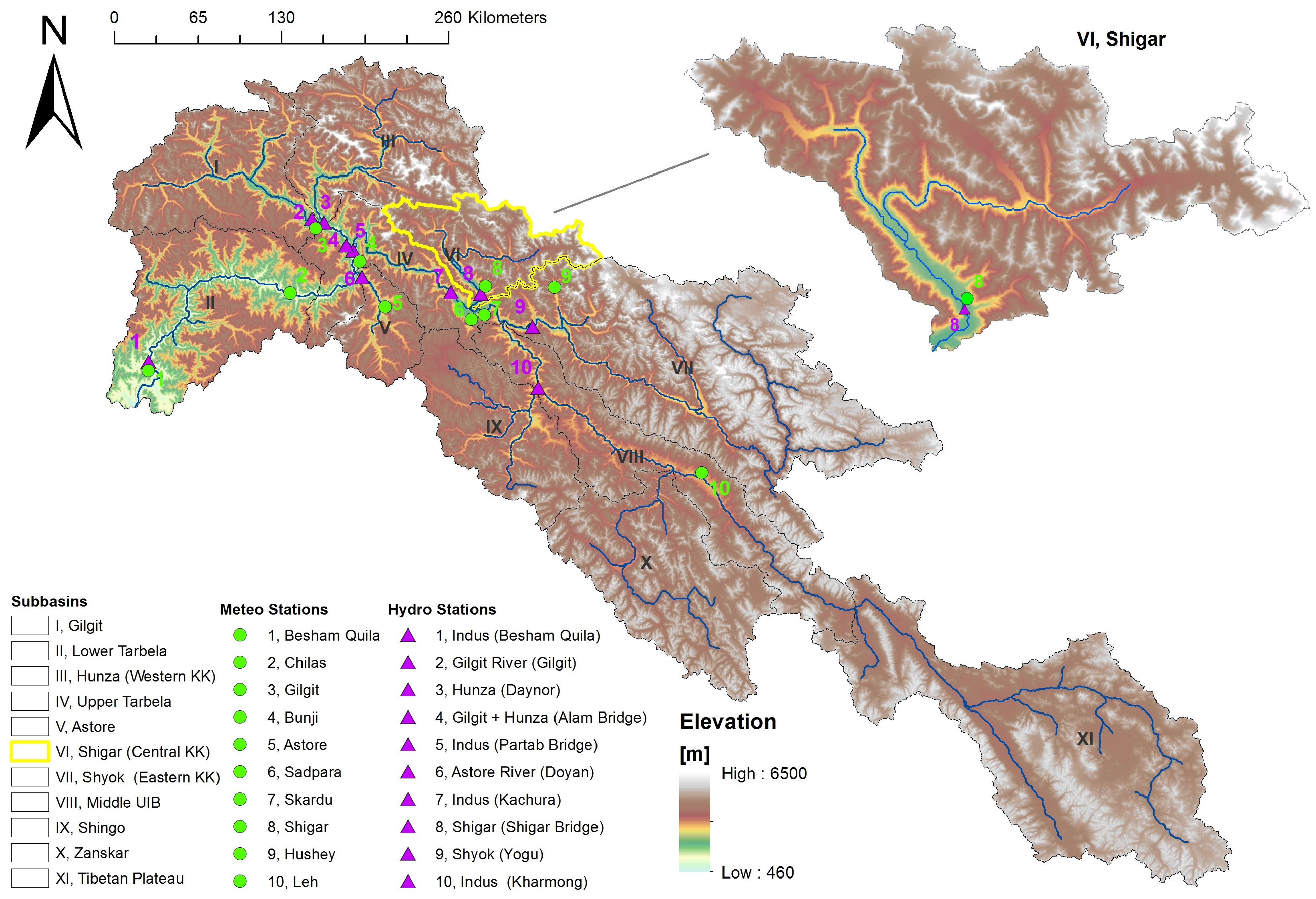
One of the principal factors hampering the hydro-glaciological analysis of this system is the inherent scarcity of ground observations needed for the validation of water balance analysis. As shown in Figure 1, the UIB is monitored by a very sparse network of precipitation, temperature and flow gauging stations with respect to its size (165,000 km${}^2$), which precludes the elaboration of reliable spatial maps of meteorological forcing across the basin necessary for hydro-glaciological mass balance studies. Moreover, precipitation and temperature are elevation dependent and, thus, characterized by strong spatial gradients over the steep surface relief. For this reason, precipitation and temperature products, which are generally derived by spatial interpolation of observations at valley stations, tend to systematically underestimate the actual meteorological variables, thus enhancing the risk of erroneous hydrological balance estimates. For example, studies of area-averaged precipitation for UIB derived from Climate Research Unit (CRU) TS3.21 [16] or the Global Precipitation Climatology Centre (GPCC) [17] precipitation analysis products have been shown [18,19] to underestimate mean annual precipitation in the UIB by approximately a factor of two.

Satellite-observed precipitation is an alternative to spatially-interpolated in situ observations. The main advantage offered by satellite measurements is the coverage of large areas and their repeatability in time. Nevertheless, satellite observations require validation against ground observations, as they may be strongly biased. For example, high-altitude applications of the TRMM 3B43 product for the wet season in the Peruvian [20] and Ecuadorian Andes [21] indicate precipitation underestimation in the order of 50%.

In view of the above-mentioned difficulties of precipitation estimation for the region of interest, the only viable alternative options for sourcing spatially- and temporally-continuous precipitation data for vast and poorly-gauged basins are atmospheric reanalyses [22]. Reanalysis data are obtained by performing runs of Global Circulation Models (GCM) at pre-defined spatial resolutions, whereby prognostic atmospheric state variables, such as temperature, wind speed, pressure and water vapor observed on the land surface or from satellites, are used to correct model simulations by means of data assimilation [23]. Through the adoption of variational principles [24] or stochastic methods [25], the atmospheric model output is adjusted so as to minimize the difference between computed variables and observations at selected time steps and measurement points. Depending on the specific reanalysis project, the atmospheric models are run over several consecutive decades, starting from the 1950s or earlier, until the present. Data assimilation has undergone progressive improvement from 1979 onwards, when satellite observations became more continuously available.

The additional benefits of using a group of atmospheric reanalyses for precipitation and temperature estimation in poorly-gauged areas arise from the simultaneous availability of multiple independent predictions, effectively an ensemble of estimators of the true atmospheric variables. Reanalyses are re-forecasts (in meteorology, also known as hindcasts) of past weather, which are inherently uncertain. A multi-model ensemble offers the possibility to quantify the Predictive Uncertainty (PU) [26,27] of the reanalysis output. Predictive uncertainty is the quantitative assessment of the predictive capability of one or multiple forecasting models to correctly estimate an observed predictand. The concept of PU applies to precipitation, temperature or any variable (re-)forecast by atmospheric reanalysis. In this context, a recent application has been presented [28] in which consistent datasets of Land Surface Temperature (LST) were generated and data gaps closed with respective uncertainty estimates by combining multiple satellite LST estimates with LST reanalyses in a Bayesian framework. Missing data were filled with the aid of the National Centre of Environmental Prediction (NCEP) Climate Forecast System Reanalysis (CFSR) product [29] by using reanalyzed LST as the predictor.

In the present application, we apply similar concepts to a different, albeit parallel setting. The unknown predictands are spatial averages of mean monthly precipitation and temperature in a poorly-gauged basin in Central Karakoram, UIB. The only supporting observations are daily precipitation and temperature observations from a single nearby ground station. The estimates of the predictand are given by series of atmospheric reanalysis data produced by independent models.

The main goals of this study are: (1) to assess the predictive uncertainty of the ensemble of atmospheric model outputs in predicting selected forcing variables; (2) to investigate to what extent the uncertainty in predicting the variable can be contained by including multiple model predictions; and (3) to perform educated gap-filling of missing ground observations. For this purpose, we adopt the Model-Conditional Processor (MCP) [30,31], which we calibrate using in situ observations. The proposed approach constitutes a systematic procedure of combining multiple atmospheric predictor variables in poorly-gauged basins to gain added information on a predictand. The specific Karakoram application presented here aims at obtaining educated guesses of basin average monthly precipitation and temperature, which can be used for improved hydrological mass balance studies, as opposed to just using unprocessed reanalyses unrelated to in situ data. As we are actually aggregating multiple model output cells to basin average variables at monthly time steps, we prefer to separate the proposed approach from statistical downscaling of GCM output to local scales [32]. While the study area we have chosen is poorly monitored and in situ observations are sparse, the methodology remains generally valid and is expected to deliver increasingly less uncertain results if ground observations become denser.

A recent study [33], which uses glacier mass balances in the UIB to inversely determine high-altitude precipitation, performed an uncertainty analysis on precipitation. Monte Carlo analysis was applied to an assumed vertical precipitation gradient model of spatially-interpolated in situ observations (APHRODITE, [34]) with prior assumptions on the statistical properties of the gradient model parameters. Such an approach requires the statistical properties and, thus, the uncertainty of precipitation to be assumed beforehand. We use reanalyses instead, which are bias-corrected and combined by weighting them on the basis of how they correlate with deterministic observations. The conceptual advantage of the latter approach is the absence of any need for making prior assumptions on the statistical properties of variables and the uncertainty, as these are a direct outcome of the Bayesian processing, as we show below.

The present contribution is structured as follows: In Section 2, we describe the study site and the data used, then we give a brief overview of the Bayesian methods of uncertainty assessment that are relevant in the context of this study. Section 3 is devoted to presenting the application of the Model-Conditional Processor (MCP) to Shigar Basin and Section 4 to discussing the results. The implementation details of the processor are reported in the Appendix.

2. Materials and Methods

2.1. Study Site

In this study, we focus exclusively on the northern region of UIB that includes the Karakoram Range. The main ridge of the Karakoram Range forms the hydrological and political divide between Pakistan and China, while the Eastern part of the study area is crossed by the Line Of Control (LOC) and is administered by India. The main tributaries originating in the area and feeding into the Upper Indus River are the rivers Hunza draining Karakoram West, Shigar draining the Central Karakoram and Shyok dewatering Karakoram East. The respective watersheds are characterized by a large portion of their area above 3500 m and are all heavily glaciated. The basin boundaries and respective areas are derived by topographic analysis of the 90 × 90 m digital elevation model derived from the Shuttle Radar Topography Mission (SRTM) dataset. The constituent major drainage units of UIB are shown in Figure 1. The glaciated areas are obtained from the Randolph Glacier Inventory Version 5.0 [35]. In the present study, we focus on the 7040-km${}^2$ Shigar Basin, which lies between the Hunza and the Shyok basins and drains the Central Karakoram. Shigar Basin is home to the large Biafo and Baltoro glaciers with a total glaciated area of 2100 km${}^2$. The hypsometric curve of Shigar Basin is given as follows: 267 km${}^2$ (3.8 %) between 2000 and 2500 m, 650 km${}^2$ (9.3 %) between 2500 and 3500 m, 1960 km${}^2$ (27.9 %) between 3500 and 4500 m, 3245 km${}^2$ (46.2 %) between 4500 and 5500 m, 811 km${}^2$ (11.4 %) between 5500 and 6500 m and 103 km${}^2$ (1.4 %) above 6500 m. The average altitude of the basin is 4579 masl.

2.2. Seasonal Precipitation and Temperature Variability in the Karakoram

The weather patterns that control precipitation in UIB and over the Karakoram are very particular. The Karakoram and Western Himalayan ranges receive heavy snowfalls during winter due to the advection of the moisture-laden mid-latitude westerly circulation and cyclonic storms from the Mediterranean, Black and Caspian seas [36,37]. These advected air masses have a major influence on regional distributions of glaciers and snow cover. About 67% of high altitude snow accumulation on central Karakoram glaciers occurs in winter [9,10,38]. Even though sub-tropical westerly jet streams cause the chief seasonal snowfall during winter with maxima in March, heavy summer snowfall at high altitudes is also prevalent in the UIB due to the incursion of monsoonal air masses from the Indian Ocean. About 33% of high altitude snow accumulation on central Karakoram glaciers occurs during the Indian monsoon period of July–September [9,10,39]. Snowfall also occurs in early summer by frontal storms drawing moisture from the Arabian Sea [40]. Since the Karakoram is located at a considerable distance from the seas and ocean, most of the moisture is transported from the west and southwest in the middle troposphere by winter westerlies. As a result, the bulk of precipitation in the Karakoram falls out at elevations higher than 4000–5000 m, in the elevation range corresponding to the accumulation zone of the major glaciers. These westerlies provide the dominant nourishment for the local glacier systems. Furthermore, there is orographic enhancement of precipitation. Although the valley floors are quite arid, precipitation amounts increase substantially with altitude [40,41] and decrease again above approximately 5500–6000 m. Actual values of total precipitation within the basin are not exactly known, but can be estimated to range between 200 mm in the arid valley bottoms (e.g., at Skardu) up to 1900 mm of water equivalent in the highest precipitation zone between 4600 and 5500 m [39,42].

At high elevations, the 2-m air temperature is sub-zero most of the year, and hence, precipitation falls there as snow. Low-end values between −20 and −30 ${}^{\circ }$C of mean monthly temperature are reached in January and maxima between +5 and +10 ${}^{\circ }$C in August at mid-altitudes around 4500 m. Due to the high elevation of the basin, the air is very dry and clear. In the rarefied atmosphere, the power of the solar radiation is very high and can cause rock surfaces to warm up to multiple tens of ${}^{\circ }$C due to exposure to direct radiation [43], while the 2-m air temperature remains below zero. This indicates a potentially strong divergence between the 2-m air temperature and LST at high altitudes in the basin. In the valley bottoms, the monthly mean temperature can vary between −10 ${}^{\circ }$C in January and approximately +28 ${}^{\circ }$C in August. We also note that given the extreme topography, local temperature is subject to strong spatial variability attributable to temperature inversions and micro-scale meteorological processes, which we will disregard in the following analysis, as we are working with monthly mean values. To give an impression of the value range of mean monthly precipitation and the 2-m air temperature in Shigar Basin in absence of within-basin in situ observations, we report the monthly climatology of precipitation and temperature spatial averages for raw unprocessed reanalysis outputs at Shigar Basin for 1979–2014 in Figure 2 and Figure 3. The processing of these reanalyses will be addressed further below.

2.3. Precipitation and Temperature Estimation in Poorly-Gauged Basins

The main challenge in performing sound hydro-glaciological assessments in poorly-monitored basins is the scarcity of reliable in situ observations. This situation is encountered in many parts of the developing world. As already indicated, satellite estimates of precipitation, such as those by TRMM, which cover a region of 50° latitude north and south of the Equator, are in principle suited to provide continuous precipitation information, but are much less reliable than for, instance, satellite-based LST estimates for our area of interest. Different studies [19,44] for the UIB indicate considerable precipitation underestimation when using satellite or interpolated ground observations. Low-density observation networks also hamper any extensive correction of TRMM precipitation measurements. Examples of satellite precipitation estimates in the UIB [45,46] with the product TRMM 2B31 yield mean annual precipitation values of 300 mm/year, which have been shown to be too low for a consistent closure of the basin water balance. Furthermore, other precipitation analysis studies in the UIB [47] reached the conclusion that TRMM measurements are a quantitative indicator of monthly rainfall abundance rather than a measure of absolute magnitude because of systematic underestimation of cumulative precipitation by 40%–60%. A comparison with atmospheric reanalyses [19] suggests that the actual mean annual precipitation for the whole UIB is more than double the TRMM estimate, ranging between 600 mm/year and 800 mm/year.

Alternatively, ensembles of atmospheric reanalyses can be used as predictors to derive the highest probability (in terms of a posterior probability distribution) estimates of area-averaged precipitation and temperature for a poorly-gauged region, such as Shigar Basin (Figure 1). The availability of an ensemble of predictors allows one to estimate and subsequently reduce the uncertainty on the predictand. This has a two-fold advantage: firstly, one obtains the most probable values to fill data gaps in the observed series; secondly, a posterior estimate of the predictand is obtained by weighting the predictors on the basis of their assessed information content. In other words, non-informative predictors are attributed less or no importance with respect to those with higher informative value. If a nearby observing station is available with the help of which an uncertainty processor can be calibrated, the suggested approach can be used to determine precipitation and temperature for a sparsely-gauged region. In the following section, we briefly discuss the most-commonly adopted methods of (re-)forecast uncertainty processing and quantification.

2.4. Approaches to Predictive Uncertainty Assessment

The use of the Bayesian paradigms for inference and prediction has become common in assessing and decreasing the uncertainty on model predictions of true variables in the fields of meteorology and weather forecasting [26,27] and more recently also river flow forecasting [48]. In this context the Predictive Uncertainty (PU) is defined as a conditional probability density:

$$PU=f(y|{\widehat{y}}_{1,t_o},{\widehat{y}}_{2,t_o},{\widehat{y}}_{3,t_o},....,{\widehat{y}}_{n,t_o})$$

(1)

where f is a conditional probability density function, y is the predictand at a given time t and ${\widehat{y}}_{i,t_o},i=1,....,n$ are n predictor variables at time t for a forecast starting at time $t_o$, which implicitly depend on a set of model parameters, θ, i.e., ${\widehat{y}}_{i,t_o}={\widehat{y}}_{i,t_o}(\mathit{\theta })$, over which we as prediction users have no influence. In a forecasting context, the chief interest lies in the assessment of PU for prediction times $t>t_o$. A re-forecast, on the other hand, as used here, reproduces the past, and thus, $t_o=t$ at each time, which is equivalent to using a lag-zero stochastic process description. Consequently, we omit the time indexing and simplify notation.

(1) The Bayesian Hydrological Uncertainty Processor (HUP) introduced by Krzysztofowicz [48,49] derives the PU as the conditional uncertainty of a predictand, conditional on a single model forecast by applying Bayes’ theorem in terms of a prior distribution (derived from climatology or a lag-n Markov chain model) and a likelihood function, which probabilistically describes model performance against observations. One of the strengths, but at the same time also a limitation of the HUP, is the analytical structure, which makes the HUP fast for operational settings, but effectively limits the application of the processor to the use of a single forecasting model. An extension of the HUP to include multiple models as predictors is not immediate within the original conceptual framework.

(2) A Bayesian uncertainty processor, which allows one to combine multiple predictors is Bayesian Model Averaging (BMA) [50,51]. In contrast to the HUP, BMA does not seek to determinate the predictive uncertainty explicitly, but evaluates an approximation of the latter in terms of a mixture of densities:

$$f(y|{\widehat{y}}_1,{\widehat{y}}_2,....,{\widehat{y}}_n)=E\{f_1(y|{\widehat{y}}_1),f_2(y|{\widehat{y}}_2),....,f_n(y|{\widehat{y}}_n)\}\approx \sum _{j=1}^n{w}_j{f}_j(y|{\widehat{y}}_j)$$

(2)

The mixture of densities is effectively the BMA mean, expressed as a linear combination of the conditional densities for individual models, where the weights $w_i$ are estimated by formulating the problem as the maximization of the log-likelihood. Once the weights are known, it is possible to estimate the predictive mean on n models as:

$$\begin{array}{ccc}\hfill E\left[y|{\widehat{y}}_1,{\widehat{y}}_2,....,{\widehat{y}}_n\right]& =& \sum _{j=1}^n{w}_j{f}_j(y|{\widehat{y}}_j)\hfill \end{array}$$

(3)

and the predictive conditional variance as a combination of the empirical mean and variance for individual models:

$$\begin{array}{ccc}\hfill Var\left[y|{\widehat{y}}_1,{\widehat{y}}_2,....,{\widehat{y}}_n\right]& \approx & \sum _{j=1}^n{w}_{j}Var(y|{\widehat{y}}_j)+\sum _{j=1}^n{w}_j{[{\widehat{y}}_j-\sum _{k=1}^n{w}_{k}E\{y|{\widehat{y}}_k\}]}^2\hfill \end{array}$$

(4)

The original version of BMA assumes a normal dependency structure between variables, but this assumption has been relaxed and successfully extended to allow for log-normal and gamma distribution dependency models [52].

(3) The third Bayesian approach to uncertainty assessment is the Model-Conditional Processor (MCP) [30]. By applying the formal definition of the conditional posterior distribution directly, the MCP includes most features of the previously-mentioned Bayesian approaches, while aiming at parsimonious parameterization. The prior distributions of both predictand and predictors are assumed equal to their climatological distributions and are mapped to the Gaussian space by means of the Normal Quantile Transform (NQT) [49]. In the normal space, the interdependency structure of predictand and predictors is assumed multivariate normal. Coccia and Todini [31] proposed an extended version of the MCP, which allows for the inclusion of multiple forecasting models with heteroscedastic dependency structures. This is relevant when dealing with variables that show residuals with varying dispersion in relation to a linear regression. Heteroscedastic dependency is typical for certain variables, such as precipitation and discharge, which exhibit non-constant variance as the magnitude of the variable increases to extreme values. A more detailed recapitulation of the MCP is provided in the Appendix.

(4) Finally, we mention uncertainty quantification by Quantile Regression (QR), an originally non-Bayesian approach, which was first used in the field of econometrics [53]. QR tries to represent the heteroscedasticity of the residuals by assuming linear or non-linear-type variation of the quantiles of the predictive uncertainty distribution, which vary with the magnitude of the predictors. The principal restriction of the QR approach is the number of parameters to be estimated, which can become large, especially when using many quantile classes. QR generally performs well if heteroscedasticity can be represented with a linear model, i.e., the residuals change linearly with the magnitude of the variable, but performs sub-optimally if this relation is non-linear, a case frequently encountered in practice at the upper and lower end of the variable range.

2.5. Atmospheric Reanalyses

For reasons given in the Introduction, we resort to an ensemble of numerical reanalyses to obtain predictors for monthly precipitation and temperature in Shigar Basin. We use the output of ongoing or recently-terminated reanalysis projects over past decades. In this analysis, we use the following six reanalysis products: (1) ERA-Interim [22]; (2) ERA20C [54]; (3) Japanese 55-year reanalysis [55]; (4) NCEP-NCAR reanalysis R1 [29]; (5) NCEP-CFSR [56]; and NASA Modern-Era Retrospective Reanalysis (MERRA) [57] (6). The products and their most important characteristics are summarized in

Table 1. Overview of the six reanalyses indicating the product name, source agency, the data range used for the analysis, model grid projection, output resolution for the analyzed fields and no. of cells used for Shigar basin. The air temperature is indicated at 2 m above ground. MERRA, Modern-Era Retrospective Reanalysis.

Dataset	Origin	Data Range	Grid Type	Spatial Res.	Temporal Res.	Cells
ERAI Reanalysis	ECMWF	1979–2014	N128 Gaussian	0.75° × 0.75° (∼79 km)	monthly means of daily means	5
NCEP/NCAR R1	NCEP/NCAR	1979–2014	1.875° × 1.875°	1.875° × 1.875° (∼209 km)	monthly	2
NASA-MERRA	NASA	1979–2014	1/2° × 2/3°	1/2° × 2/3° (∼55 × 73 km)	monthly means	7
NCEP CFSR	NCEP	1979–2009	T382 Gaussian	0.313° × 0.313° (∼38 km)	monthly	17
55-y Japanese Reanalysis	Jp.Met. Agency	1979–2014	TL390L60	1.25° × 1.25° (∼135 km)	monthly means	4
ERA 20C Reanalysis	ECMWF	1979–2010	N80 Gaussian	1.0° × 1.0° (∼125 km)	monthly means of daily means	4

. In this analysis, we focus on two output variables: 2-m air temperature, a prognostic variable, as well as precipitation, a diagnostic variable. We have selected the most contemporary reanalysis products developed by source organizations, which apply different models and data assimilation procedures to obtain a six-member ensemble of independent physically-based estimates of the variables of interest. For reasons of consistency, only data from 1979 onwards are used. Most atmospheric reanalyses reach as far forward as the second decade of the 21st century or are still ongoing.

The meteorological data, precipitation and 2-m air temperature are spatially averaged over the Shigar Basin area, indicated with a yellow boundary and magnified in the excerpt in Figure 1. The reanalysis outputs have different spatial resolutions and, therefore, involve a varying number of grid cells. The averaging procedure requires the calculation of the weighted mean of the respective variable X using the sub-basin mask to identify the relevant model cells. All reanalysis cells that overlap with the area enclosed by the mask are used to perform the averaging. The average $\overline{X}$ is given by the area-weighted average precipitation:

$${\overline{X}}^j=\frac{{\sum }_{i=1}^n{X}_i^j·A_i}{A_{tot}}$$

(5)

where the index i indicates cell i, j indicates the monthly time step, $A_i$ is the basin area portion covered by the i-th reanalysis pixel, $A_{tot}$ is the sub-basin area and n is the total number of cells found within the sub-basin mask. The resulting series of basin average data for each reanalysis series are assumed to hold approximately at the basin centroid with elevation 4579 m.

2.6. Meteorological In Situ Observations

Only a few precipitation and temperature gauges are operated continuously in UIB and are located mainly in the valleys, in the proximity of settlements. Most of the remote mountainous high-altitude areas are not covered by any observing networks. Few precipitation stations have been operated at relatively higher elevations. These so-called “high-altitude stations” have been operational only since 1994 or later years. In addition, some special research projects led to the temporary dispatch of automatic weather stations, which were removed after a few seasons and the wrap-up of the project [39,58,59,60]. Such data are important to assess local precipitation and temperature distributions over altitude, but cannot be employed for any trend analysis on water flow or ice mass development due to the brevity of the records. In the present example of Shigar Basin, there are very few nearby ground stations for temperature and precipitation available.

The most reliable station is Skardu situated in the Indus Valley, in the proximity of the Shigar-Indus River confluence. The station has been operated with brief interruptions over more than a century since 1894. We use the mean monthly precipitation and temperature records from 1951 onwards. A second precipitation station is located at Shigar village within the basin. This station has a record length of less than 20 years since 1996. A statistical analysis of mean monthly values has shown that the series at Shigar village do not correlate with Skardu (

Table 2. Position and elevation of recording stations for precipitation, record length and correlations with Skardu station.

Station	Position	Elevation masl	Period	Correlation
Skardu	35°17${}^{\prime }$01${}^{″}$ N, 75°38${}^{\prime }$32${}^{″}$ E	2210 m	1952–2014	1.00
Shigar (village)	35°25${}^{\prime }$19${}^{″}$ N, 75°44${}^{\prime }$20${}^{″}$ E	2294 m	1996–2012	0.16
Sadpara (Deosai)	35°14${}^{\prime }$40${}^{″}$ N, 75°38${}^{\prime }$07${}^{″}$ E	2660 m	1995–2011	0.54
Hushey	35°26${}^{\prime }$60${}^{″}$ N, 76°21${}^{\prime }$53${}^{″}$ E	3148 m	1994–2010	0.26

), most likely due to the orography. Two more stations are located at Sadpara lake (Deosai) and Hushey village. These stations, albeit close to Skardu in straight-line distance, are situated in the Indus Valley and the Shyok Basin and have records starting in 1995 and 1994, respectively. Sadpara (Deosai) correlates reasonably well with Skardu, while Hushey correlates also very poorly (Table 2). Closer examination of the station in Hushey indicates that the station does not deliver a reliable record, especially between 2001 and 2004.

We also performed a double mass curve analysis between Skardu and the three neighboring stations with shorter records to examine the reliability of the stations for the 1996–2012 period. The results are reported in Figure 4.

Given the evidently poor mutual consistencies in terms of cumulative recorded volume, especially concerning Shigar station, we decided to discard the three shorter records and to retain the Skardu record only. This record is also reasonably complete, with only 3% of data missing between 1979 and 2014. Skardu precipitation and temperature records require correction to values that reflect the higher mean elevation of Shigar Basin. This can be achieved by applying vertical precipitation and temperature gradients. Similar to [61], a precipitation gradient reported in the literature [60,62] for the Central Karakoram can be applied. An empirical expression is given by the following power law, which holds for the elevation range 2000–5500 m, beyond which precipitation starts to decline with altitude:

$$P_z[mm/y]=9·{10}^{-6}·z^{2.22}$$

(6)

This relationship is integrated over the hypsographic curve of the basin for h ≤ 5500 m and yields an areal annual increase of total precipitation equal to 907 mm/year:

$$\Delta P_{corr}[mm/y]=9·{10}^{-6}·\frac{1}{A}{\int }_{h_{Skardu}}^{h_{centroid}}{z}^{2.22}dA(z)\approx 9·{10}^{-6}·\frac{1}{A}\sum _{i=1}^n{h}_i^{2.22}{A}_i$$

(7)

with $A_i$ the area of a DEM pixel, $h_i$ its elevation with respect to Skardu and n the number of pixels. Because the relationship is expressed as an annual increase, no distinction can be made for individual months, and one obtains a uniform correction factor of 4.9 mm, which we apply to Skardu mean monthly precipitation to account for orographic effects. However, if a time-varying scaling relationship with different values for each month would be available, it could be used in the proposed approach. In absence of such a relationship, we are forced to proceed with a constant scaling coefficient. While this scaling approach may seem crude, we recall that we are working in a poorly-monitored environment and focus on mean monthly values. The precipitation climatology and the corrected monthly precipitation for each month are summarized in

Table 3. Monthly precipitation climatology at Skardu, 1951–2012, the fraction of annual mean precipitation and corrected monthly precipitation to account for elevation change from 2210 m to 4579 m.

	J	F	M	A	M	J	J	A	S	O	N	D	Tot
P(mm)	30	29	39	33	30	9	11	13	10	8	5	17	233
P/P${}_{yr}$	0.13	0.12	0.17	0.14	0.13	0.04	0.05	0.06	0.04	0.03	0.02	0.07	1.0
$\Delta P_{corr}$ (mm)	116	112	152	127	114	35	44	50	39	31	21	65	907
P${}_{corr}$ (mm)	147	142	193	161	145	44	56	64	50	40	26	83	1152

.

For temperature, the adiabatic lapse rate can be integrated over the hypsographic curve to scale from the ground elevation at Skardu to the altitude of the basin mean elevation:

$$dT/dz({}^{\circ }C/km)=-6.4$$

(8)

In principle, the lapse rate varies between months, but also here, we need to resort to an mean annual rate due to the lack of data. We note that the application of the temperature lapse rate at Skardu is equivalent to bias-correcting the data with respect to the basin centroid by a constant shift. As will become clear further below, the Model-Conditional Processor (MCP), which we use for the Bayesian combination of observations with reanalysis data in Section 3, neglects a bias between observations and predictor variables, as correlations between variables are invariant to constant shifts. Therefore, it suffices to correct the already processed temperature by adding a constant value of −15.2 °C. This consideration does not apply to precipitation that needs to be rescaled by multiplication with the correction factor ahead of processing. In this context, we also note that given the coarse spatial resolution of the reanalysis data and the smoothing of the underlying elevation grid of the atmospheric model, there is also some uncertainty as to which actual mean elevation basin average data (see Equation (5)) they relate.

3. Application of the Model-Conditional Processor

3.1. Normalization of Variables

From the predictive uncertainty assessment approaches mentioned in Section 2.4, we resort to the Multi-Conditional Processor (MCP) to derive the probability distribution for monthly mean areal precipitation and temperature at Shigar given six reanalysis series. The series cover different lengths, as indicated in Table 1. For our study, we select the period 1979–2009, adapting to the shortest available series (CFSR) as our reference period. The processing of the data is executed in consecutive steps. First, we transform the altitude-corrected series of monthly precipitation and temperature observed at Skardu into the Gaussian normal space using the Normal Quantile Transform (NQT). The same is done for the predicted series of the six reanalysis models. The transformed observations at time t are denoted with η and the transformed model predictions with ${\widehat{\eta }}_i$, where $i=1,...,n$ is an index sweeping the different atmospheric reanalysis outputs. Both transformed variables are standard normal N(0,1).

3.2. Precipitation: Normal Distributions

We refer to the notation introduced in the Appendix, which indicates realizations at time t of the random process η and ${\widehat{\mathit{\eta }}}_i$ as η, respectively ${\widehat{\eta }}_i$. Figure 5 shows the NQT-transformed empirical $\eta -{\widehat{\eta }}_i$ relationships as scatterplots for all six reanalysis re-forecasts. One needs to envisage these scatterplots as the projection of the multivariate-normal dependency ($\eta ,{\widehat{\eta }}_i),i=1,...,n$ onto the respective $\eta -{\widehat{\eta }}_i$ plane as a bivariate-normal process $(\eta ,{\widehat{\eta }}_i)$. We note that in all plots, there are no data points for $\eta <-1.36$, because precipitation is always non-negative. The red solid line indicates the 50% quantile or conditional median obeying the linear relationship $\eta |{\widehat{\eta }}_i({\widehat{\eta }}_i)={\rho }_{\mathit{\eta }{\widehat{\mathit{\eta }}}^n}·{\widehat{\eta }}_i+{\mu }_{\eta }$ with ${\mu }_{\eta }=0$, while expectation and variance are equal to:

$$\begin{array}{ccc}\hfill E(\eta |{\widehat{\eta }}_i)& =& {\mu }_{\eta |{\widehat{\eta }}_i}={\rho }_{\mathit{\eta }{\widehat{\mathit{\eta }}}^n}·{\widehat{\eta }}_i\hfill \end{array}$$

(9)

$$\begin{array}{ccc}\hfill Var(\eta |{\widehat{\eta }}_i)& =& {\sigma }_{\mathit{\eta }|{\widehat{\mathit{\eta }}}_i}^2=1-{\rho }_{\mathit{\eta }{\widehat{\mathit{\eta }}}_i}^2\hfill \end{array}$$

(10)

where ${\mu }_{\eta |{\widehat{\eta }}_i}$ is the conditional mean and ${\rho }_{\mathit{\eta }{\widehat{\mathit{\eta }}}_i}$ is the correlation. We note that in the normal space, the conditional median coincides with the conditional mean and the conditional modal value. The red dashed lines indicate the 90% credible interval and are at a parallel distance of two standard deviations from the mean. The parametric conditional normal density for a single predictor ${\widehat{\eta }}_i$ is given by the expression:

$$\varphi (\eta |{\widehat{\eta }}_i)=\frac{exp[-\frac{1}{2}(\eta -{\mu }_{\eta |{\widehat{\eta }}_i}{)}^2/(1-{\rho }_{\mathit{\eta }{\widehat{\mathit{\eta }}}_i}^2)]}{\sqrt{2\pi ·(1-{\rho }_{\mathit{\eta }{\widehat{\mathit{\eta }}}_i}^2)}}$$

(11)

We note that the conditional variance ${\sigma }_{\mathit{\eta }|{\widehat{\mathit{\eta }}}_i}^2=(1-{\rho }_{\mathit{\eta }{\widehat{\mathit{\eta }}}_i}^2)$ is at the denominator, and thus, with ${\rho }_{\mathit{\eta }{\widehat{\mathit{\eta }}}_i}\to 1$ and ${\sigma }_{\mathit{\eta }|{\widehat{\mathit{\eta }}}_i}^2\to 0$, the conditional density curve becomes steeper with probability narrowly concentrated. This is tantamount to minimizing the predictive uncertainty by using an increasingly “optimal” model. As described in more detail in the Appendix, the conditional density can be extended to include all six reanalyses as conditioning variables, leading to the following parametric multi-normal density of η, conditional on n potential predictors:

$$\varphi (\eta |{\widehat{\eta }}_1,....,{\widehat{\eta }}_n)=\frac{exp[-\frac{1}{2}{(\eta -{\mu }_{\eta |{\widehat{\eta }}^n})}^2/{\sigma }_{\mathit{\eta }|{\widehat{\mathit{\eta }}}^n}^2]}{\sqrt{2\pi }·{\sigma }_{\mathit{\eta }|{\widehat{\mathit{\eta }}}^n}}$$

(12)

where conditional mean and variance are expressed in terms of the $(n+1)\times (n+1)$-dimensional variance-covariance matrix ${\mathit{C}}_{\mathit{\eta },{\widehat{\mathit{\eta }}}^n}$ with sub-matrices ${\mathit{C}}_{\mathit{\eta }{\widehat{\mathit{\eta }}}^n}$ and ${\mathit{C}}_{{\widehat{\mathit{\eta }}}^{\mathit{n}}{\widehat{\mathit{\eta }}}^{\mathit{n}}}$:

$$\begin{array}{ccc}\hfill {\mu }_{\eta |{\widehat{\eta }}^n}& =& {\mathit{C}}_{\mathit{\eta }{\widehat{\mathit{\eta }}}^n}·{\mathit{C}}_{{\widehat{\mathit{\eta }}}^{\mathit{n}}{\widehat{\mathit{\eta }}}^{\mathit{n}}}^{-\mathbf{1}}·{\widehat{\eta }}^n\hfill \end{array}$$

(13)

$$\begin{array}{ccc}\hfill {\sigma }_{\mathit{\eta }|{\widehat{\mathit{\eta }}}^n}^2& =& 1-{\mathit{C}}_{\mathit{\eta }{\widehat{\mathit{\eta }}}^n}·{\mathit{C}}_{{\widehat{\mathit{\eta }}}^{\mathit{n}}{\widehat{\mathit{\eta }}}^{\mathit{n}}}^{-\mathbf{1}}·{\mathit{C}}_{\mathit{\eta }{\widehat{\mathit{\eta }}}^n}^T\hfill \end{array}$$

(14)

In Equation (12), the variance-covariance matrix combines n different models with observations. The covariances are evaluated over a sufficiently long calibration period, for which predictions, as well as observations are available, and specify the added value of the different forecast models by weighting the predictor variables ${\widehat{\mathit{\eta }}}^n$ accordingly in the conditional variance ${\sigma }_{\mathit{\eta }|{\widehat{\mathit{\eta }}}^n}^2$. Model forecasts that correlate poorly with the predictand are weighted lower with respect to those with higher correlation. Equation (12) is the marginalization of the multi-normal density $\varphi (\eta ,{\widehat{\eta }}_1,....,{\widehat{\eta }}_n)$ defined in an $(n+1)$-dimensional data space. In case a homoscedastic dependence structure $(\eta ,{\widehat{\eta }}_i)$ can be assumed between variables, Equations (12)–(14) apply over the entire value range of ${\widehat{\eta }}_i$.

3.3. Precipitation: Multivariate Truncated Normal Distributions

For all subplots in Figure 5, we note a higher spread of the normalized data for lower precipitation values, an indication that the assumption of homoscedasticity of the residuals between the normalized data point and the linear regression does not hold. To address this issue, it is necessary to model the relationship between transformed observations and predictions via a Multivariate Truncated Normal Distribution (MTND) by subdividing the domain of the variable ${\widehat{\eta }}_i$ into two sub-domains, in which the dependency between η and ${\widehat{\eta }}_i$ can be assumed approximately homoscedastic. The verification of the homoscedasticity of the residuals needs to be performed separately between the observations and the different models. For a given predictor, one identifies a threshold value ${\widehat{\eta }}_i^{*}=a_i$ and two truncated multi-normal distributions, which are valid for $-\infty <{\widehat{\eta }}_i\le a_i$ and for $a_i<{\widehat{\eta }}_i<\infty$. In the multi-model case, for which $i=1,...,n$, and the bisection of the interval, there are $2^n$ MTNDs with separating threshold values $a_i$. The truncated conditional densities are normal $N({\mu }_{\eta },{\sigma }_{\mathit{\eta }|{\widehat{\mathit{\eta }}}^n})$, with mean and variances given as follows [63]:

$$\begin{array}{ccc}\hfill {\mu }_{\eta |{\widehat{\eta }}^n={\widehat{\eta }}^{n,*},{\widehat{\eta }}_i^{*}>a_i,i=1,...,n}& =& \mu +{\mathit{C}}_{\mathit{\eta }{\widehat{\mathit{\eta }}}^n}·{\mathit{C}}_{{\widehat{\mathit{\eta }}}^{\mathit{n}}{\widehat{\mathit{\eta }}}^{\mathit{n}}}^{-\mathbf{1}}·({\widehat{\eta }}^n-{\widehat{\mu }}^n)\hfill \end{array}$$

(15)

$$\begin{array}{ccc}\hfill {\sigma }_{\mathit{\eta }|{\widehat{\mathit{\eta }}}^n={\widehat{\mathit{\eta }}}^{n,*},{\widehat{\mathit{\eta }}}_i^{*}>a_i,i=1,...,n}^2& =& {\mathit{C}}_{\mathit{\eta }\mathit{\eta }}-{\mathit{C}}_{\mathit{\eta }{\widehat{\mathit{\eta }}}^n}·{\mathit{C}}_{{\widehat{\mathit{\eta }}}^{\mathit{n}}{\widehat{\mathit{\eta }}}^{\mathit{n}}}^{-\mathbf{1}}·{\mathit{C}}_{\mathit{\eta }{\widehat{\mathit{\eta }}}^n}^T\hfill \end{array}$$

(16)

for the upper segment and:

$$\begin{array}{ccc}\hfill {\mu }_{\eta |{\widehat{\eta }}^n={\widehat{\eta }}^{n,*},{\widehat{\eta }}_i^{*}\le a_i,i=1,...,n}& =& \mu +{\mathit{C}}_{\mathit{\eta }{\widehat{\mathit{\eta }}}^n}·{\mathit{C}}_{{\widehat{\mathit{\eta }}}^{\mathit{n}}{\widehat{\mathit{\eta }}}^{\mathit{n}}}^{-\mathbf{1}}·({\widehat{\eta }}^n-{\widehat{\mu }}^n)\hfill \end{array}$$

(17)

$$\begin{array}{ccc}\hfill {\sigma }_{\mathit{\eta }|{\widehat{\mathit{\eta }}}^n={\widehat{\mathit{\eta }}}^{n,*},{\widehat{\mathit{\eta }}}_i^{*}\le a_i,i=1,...,n}^2& =& {\mathit{C}}_{\mathit{\eta }\mathit{\eta }}-{\mathit{C}}_{\mathit{\eta }{\widehat{\mathit{\eta }}}^n}·{\mathit{C}}_{{\widehat{\mathit{\eta }}}^{\mathit{n}}{\widehat{\mathit{\eta }}}^{\mathit{n}}}^{-\mathbf{1}}·{\mathit{C}}_{\mathit{\eta }{\widehat{\mathit{\eta }}}^n}^T\hfill \end{array}$$

(18)

for the lower segment. The quantities μ, ${\widehat{\mu }}^n$ are, respectively, the sample means of η and ${\widehat{\mathit{\eta }}}^n$, while ${\mathit{C}}_{\mathit{\eta }\mathit{\eta }}$, ${\mathit{C}}_{{\widehat{\mathit{\eta }}}^{\mathit{n}}{\widehat{\mathit{\eta }}}^{\mathit{n}}}$ and ${\mathit{C}}_{\mathit{\eta }{\widehat{\mathit{\eta }}}^n}$ are the components of the covariance matrix of η and ${\widehat{\mathit{\eta }}}^n$. The values of the thresholds $a_i$ are identified with an automated search procedure, in which the variance of the upper segment, which corresponds to high precipitation values, is minimized. The search interval is limited on both ends to ensure that the upper and the lower sample is of sufficiently large size to calculate statistically-meaningful moments of the truncated distributions. For additional details on the MTDNs application, the reader is referred to Coccia and Todini [31]. In the lower four subplots of Figure 3, the change between the MTND is visible through the slope change of the median line and the more adherent 90% confidence interval in the upper data samples. In the upper two plots, which show the NQTs for ERAIand ERA20C, the processor did not succeed to break the interval into two components while retaining sufficient sampling points in each. In this case, the dependence was modeled with a simple multivariate normal.

3.4. Temperature: Multivariate Normal Distributions

Figure 6 shows the NQT-transformed temperature data. In this case, we note that the process $(\eta ,{\widehat{\eta }}_i),i=1,...,n$ is homoscedastic in all six cases. This is mainly due to the much higher predictability of temperature as a prognostic variable by the atmospheric models with respect to precipitation. Temperature is a primary variable governed by the energy conservation equation for air. Precipitation, on the other hand, is derived diagnostically using water vapor and temperature to drive a parameterized cloud sub-model, which makes this variable considerably less predictable. Given the evidently homoscedastic behavior of residuals, it is unnecessary to apply MTND because a uniform conditional variance value holds over the entire data range.

3.5. Inverse Transform and Correlation Analysis

As the next step, we perform the inverse NQT transformation of the normal densities back into the original space. Explicitly, $\varphi (\eta ,{\widehat{\eta }}_i)$ and $\varphi (\eta |{\widehat{\eta }}_i)$ are transformed back into $f(y,{\widehat{y}}_i)$ and $f(y|{\widehat{y}}_i)$. We note that in the original space, median, mode and mean no longer coincide. To examine the performance of the processor, we calculate the correlations of individual predictions against observations. These are summarized in

Table 4. Correlations between observations vs. raw predictions and observations vs. the posterior conditional mean; individual model predictions ${\widehat{y}}_i$ and the combination of predictions; precipitation and temperature.

Variable	Correlation	ERAI	ERA20C	MERRA	NCAR R1	CFSR	JRA55	All Combined
P	$corr(y,{\widehat{y}}_i)$	0.65	0.56	0.63	0.58	0.62	0.67	-
P	$corr(y,E[y|{\widehat{y}}_i])$	0.67	0.54	0.62	0.58	0.61	0.67	0.68
T	$corr(y,{\widehat{y}}_i)$	0.75	0.94	0.66	0.78	0.97	0.62	-
T	$corr(y,E[y|{\widehat{y}}_i])$	0.90	0.96	0.94	0.93	0.98	0.95	0.98

for precipitation (Line 1) and temperature (Line 3) observations and raw unprocessed model predictions by individual models. For precipitation and raw model output, the correlation varies among models and is highest for JRA55and ERAI. Recalling Table 2, we also note that the observations at Skardu correlate better with all six raw reanalysis predictions than with data recorded at neighboring stations, which further substantiates our decision to use only Skardu observations to condition the processor.

After application of the processor, we calculate the correlation (Line 2) between observations and the mean of the posterior distribution (i.e., predictive uncertainty) conditional on (1) individual models and (2) on the Bayesian combination of the ensemble of all six models. In Case (1), the correlation improves only minimally and notably most for ERAI. In the other cases, they remain equal or deteriorate, indicating that the precipitation predictions are essentially of limited informative value. For Case (2), in which all six models are combined, the correlation improves only slightly with respect to the best performing individual model JRA55 to an overall maximum value of 0.68.

The picture for temperature is completely different and considerably brighter (Line 4). In this case the processor yields an improved posterior correlation with the conditional mean. The prior correlation between observations and raw predictions is highest for ERA20C (0.94) and CFSR (0.97). In Case (1), the correlation with posterior conditional means improves notably for all temperature predictions and is highest for CFSR with a correlation reaching a value as high as 0.98, while the highest improvement has been achieved with JRA55 where the correlation jumps from 0.62 to 0.95 through processing. For Case (2), i.e., the Bayesian combination of all six models, the correlation does not improve beyond the 0.98 already achieved for CFSR.

3.6. Reconstruction of Observation Gaps

We recall that approximately 3% of the data in the observations series of precipitation at Skardu is missing, while the temperature series is complete. We can now use the expected value conditional on model predictions, $E[y|{\widehat{y}}_i],i=1,...,n$, in correspondence with the data gaps to perform an educated missing value reconstruction. The processor delivers the most probable monthly mean value of precipitation or temperature observed at Skardu, conditional on six independent reanalysis predictions, including an estimate of the variance. This example shows how the processor serves as a powerful application for educated data reconstruction by the Bayesian combination of model estimates as prior information.

Table 5. Mean annual precipitation for 1979–2009 observed at Skardu, individual model predictions and the combination of predictions. The first row contains annual means of Skardu observations and unprocessed predictions. The second row contains annual means of conditional means. We note the adjustment for elevation in the processed predictions and observations.

P${}_{\mathit{annual}}$	Skardu Obs.	ERAI	ERA20C	MERRA	NCAR R1	CFSR	JRA55	All Comb.
$<{\widehat{y}}_i>$	241	708	450	1034	594	1021	979
$<E[y|{\widehat{y}}_i]>$	1116	1209	1026	1103	1041	1048	1072	1153

, first row, lists the annual means for 1979–2009 raw predictions for individual models and the Bayesian combination of all models in the last column of the table. The second row shows the results of the processing of predictions, conditioned on elevation-corrected observations at Skardu as annual means of conditional mean precipitation at the basin centroid, 4579 m.

Figure 7 shows the entire gap-filled series of monthly altitude-adjusted precipitation observations (red line), including reconstructed values (3% in total) in correspondence with the Shigar Basin centroid at 4579 masl. The shaded area indicates the uncertainty band drawn from the conditional posterior density of the combined reanalyses. Figure 8 is the analogous plot for temperature showing a much narrower uncertainty bandwidth than precipitation. We note that for temperature, there are no measurement gaps. Although uncertainty is much narrower for temperature than for precipitation, it still remains very high, as uncertainty of up to 5 °C can have very important impacts on glacier mass balance and snow cover, especially for temperatures around 0 °C. However, this becomes less of an issue in the case that the combined series are used for trend analysis of temperature.

4. Discussion

4.1. Performance Indicators

The performance of the processor and the added value by individual models towards reducing predictive uncertainty needs to be examined by means of indicators evaluated in the normal space, which quantify the skill of each single prediction and of the combination of all six predictions. As can be seen from a visual inspection of Figure 5 and Figure 6, the prediction of precipitation is much more difficult than the one of temperature. This is visible from the wide spread and heteroscedastic dependence structure of observations and predictions in the normal space.

A first quantitative indicator of performance is the intercomparison of the correlations of observed and predicted monthly means shown in Table 4. A more in-depth analysis of processor performance can be obtained by looking at the correlation and variance of the residuals.

Table 6. Precipitation: summary of variance analysis after uncertainty processing for individual models and the combination of all models.

Quantity	Def.	ERAI	ERA20C	MERRA	NCAR R1	CFSR	JRA55	All Comb.
correlation	${\rho }_{\eta {\widehat{\eta }}_i}$	0.69	0.62	0.62	0.60	0.58	0.68	0.72
var.residuals	$1-{\rho }_{\eta {\widehat{\eta }}_i}^2$	0.50	0.58	0.60	0.62	0.64	0.52	0.47
explained var.	${\rho }_{\eta {\widehat{\eta }}_i}^2$	0.46	0.36	0.37	0.35	0.32	0.45	0.51
frac.var. unexpl.	$(1-{\rho }_{\eta {\widehat{\eta }}_i}^2)/{\sigma }_{{\widehat{\eta }}_i}^2$	0.52	0.62	0.62	0.64	0.67	0.54	0.48
frac. var. expl.	${\rho }_{\eta {\widehat{\eta }}_i}^2/{\sigma }_{{\widehat{\eta }}_i}^2$	0.48	0.38	0.38	0.36	0.33	0.46	0.52
signal/noise	${\rho }_{\eta {\widehat{\eta }}_i}^2/(1-{\rho }_{\eta {\widehat{\eta }}_i}^2)$	0.94	0.63	0.63	0.57	0.50	0.88	1.10
bias		−36.91	−59.13	−8.90	−46.38	−11.00	−14.79	0.05
RMS		9.96	10.33	9.66	10.10	9.68	9.77	9.26

shows an overview of the correlations, the variance of the residuals (also called variance unexplained), the variance explained, bias and RMSE. The first is an overall indicator of the Gaussian scatter around the linear regression model, while the latter is the variance, which can be explained solely by the regression model. In addition, we calculate the fractions of variance explained and variance unexplained, to show the percentages of each. As can be seen in the table, all six models have a correlation with observations of approximately 0.6. The combination of all models increases the correlations to a value of 0.72, proving that there is a net added informative value in combining all six predictions. However, the fraction of variance unexplained is in all cases higher or equal to 50% of total variance, which shows that the precipitation is not reliably predicted by any of the six reanalysis models, nor their combination.

Next, we report the “signal-to-noise” ratio, a decision-theoretic measure of the informativeness of output [48] for individual models and the combination of all models. It shows values that are minimal for R1 and CFSR and highest for JRA55 and ERAI. The combination of models brings the ratio to a value of 1.10, indicating that the co-processing of all models leads to an improvement by a factor of 2.2 with respect to the worst performing predictor (CFSR) when processed as a single model. In the hypothetical case of a totally uninformative model, which would be completely uncorrelated with observations, i.e., ${\rho }_{\eta {\widehat{\eta }}_i}=0$, the total variance becomes unexplained, and the signal-to-noise ratio ${\rho }_{\eta {\widehat{\eta }}_i}^2/(1-{\rho }_{\eta {\widehat{\eta }}_i}^2)$ drops to zero. To the contrary, if the model is “perfect”, ${\rho }_{\eta {\widehat{\eta }}_i}=1$, and the signal-to-noise ratio $\to \infty$. Since for all individual models, the noise exceeds the signal, no robust conclusions can be drawn from the results for individual models, and only slight gains are obtained for the combination of all models. Given that we are using monthly precipitation, we can safely assume that the predictive capacity of the models further decreases for sub-monthly temporal resolution.

The last two lines of the table report the bias and the root mean square error. We note that the effect of the MCP is the removal of the bias, which reduces to near zero after processing. The RMSE however remains nearly unchanged as high before and after processing, which in this case is due to poor predictability of precipitation.

The same performance indicators for temperature are reported in

Table 7. Temperature: summary of the variance analysis of the normal standard transformed variables after uncertainty processing for individual models and the combination of all models.

Quantity	Def.	ERAI	ERA20C	MERRA	NCAR R1	CFSR	JRA55	All Comb.
correlation	${\rho }_{\eta {\widehat{\eta }}_i}$	0.95	0.94	0.95	0.92	0.96	0.95	0.97
var. residuals	$1-{\rho }_{\eta {\widehat{\eta }}_i}^2$	0.10	0.11	0.09	0.15	0.08	0.09	0.06
explained var.	${\rho }_{\eta {\widehat{\eta }}_i}^2$	0.88	0.86	0.89	0.83	0.89	0.88	0.91
frac. var. unexpl.	$(1-{\rho }_{\eta {\widehat{\eta }}_i}^2)/{\sigma }_{{\widehat{\eta }}_i}^2$	0.10	0.11	0.09	0.15	0.09	0.09	0.06
frac. var. expl.	${\rho }_{\eta {\widehat{\eta }}_i}^2/{\sigma }_{{\widehat{\eta }}_i}^2$	0.90	0.89	0.91	0.85	0.91	0.81	0.94
signal/noise	${\rho }_{\eta {\widehat{\eta }}_i}^2/(1-{\rho }_{\eta {\widehat{\eta }}_i}^2)$	8.99	7.77	9.84	5.53	10.61	10.05	15.05
bias		−24.36	−22.84	−20.27	−19.71	−20.13	−19.20	0.092
RMSE		1.51	1.87	1.54	1.74	1.51	1.52	1.26

. As to be expected, the values of the correlations are above 0.9, showing an excellent correspondence between observations and predictions for all models. The fraction of variance of residuals is in the order of 10% and, thus, relatively small. For the combination of all models’ cases, the signal exceeds noise by a factor of approximately 15. In this case, JRA55 and CFRS turn out to be the most reliable predictions, while NCEP/NCAR R1 is the least reliable. The low performance of the latter could among other reasons be related to the much coarser spatial resolution of the R1 model grid with respect to the other products (see Table 1). For temperature, the bias is much lower and reduces to near-zero after processing. As to be expected, for temperature, the RMSE is also low for all cases.

4.2. Residuals and Reliability

Finally, we examine the probability distribution of residuals for the combination of all models in the normal space. We compare the empirical distribution with the parametric normal distribution N(0,$1-{\rho }_{\eta {\widehat{\eta }}_i}^2$). The results for precipitation are reported in the left pane of Figure 9, while those of temperature in Figure 8. We see that both empirical distributions provide a near-perfect match with the parametric model in absence of any bias. Only the distribution of residuals of precipitation is departing slightly from the parametric curve in the lower-end tail, which is exclusively caused by the high spread of predicted precipitation in the low range, also visible in the scatterplots of Figure 5. For temperature, the match with the parametric curve is near-perfect.

The performance of the processor can also be presented in synthetic fashion through reliability diagrams or quantile-quantile plots shown for precipitation and temperature in the right panes of Figure 9 and Figure 10, respectively. These diagrams are the most important rapid-assessment tool for validating the correctness of the approach. The diagrams show 5% percentage bins of monthly precipitation and temperature observations y against the 5% credibility quantiles around the expected value $E[y|{\widehat{y}}_i],i=1,...,n$ estimated by the processor for all models combined. Perfect behavior corresponds to red dots lying on the bisection line, indicating a perfect match of the percentages of observations that fall within each uncertainty quantile bin. In the case of precipitation, we see a clear departure from the bisection in the 20% quantile, while the behavior improves for higher quantiles. This is mainly attributable to poor reanalysis results in the low monthly precipitation range. For temperature, the points are reasonably well and symmetrically aligned with the bisection line, indicating much better correspondence between processed predictions and observations.

Finally, we note that our samples are uncensored. By censoring the raw precipitation data and eliminating heavy outliers, an improved performance of the processor can be achieved. To further improve processor performance, we can separate the raw precipitation data into months or three-monthly seasons with their specific precipitation regime. For instance, in the Karakoram, precipitation falls mainly in winter and during the summer monsoon season. This recurring pattern can be used as guidance to separate the original sample. On the other side, given the relatively short period of monthly data, splitting the original sample leads to even shorter sub-samples, which reduce the reliability of the statistics.

5. Conclusions

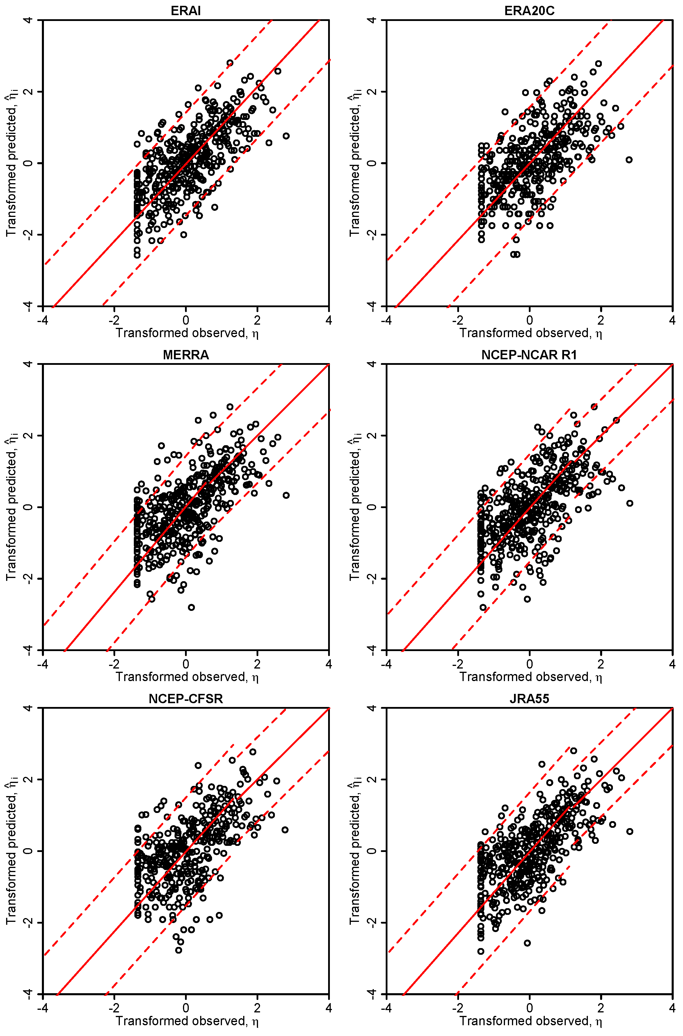
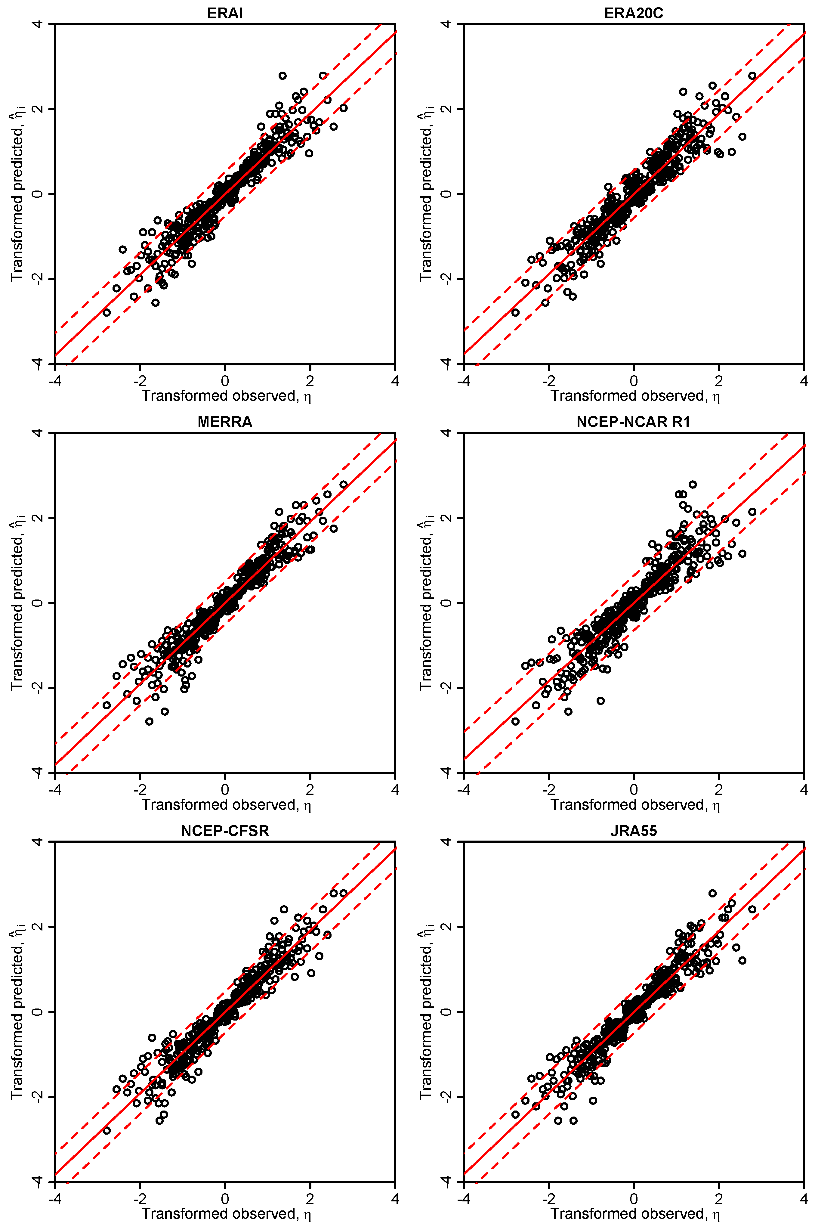
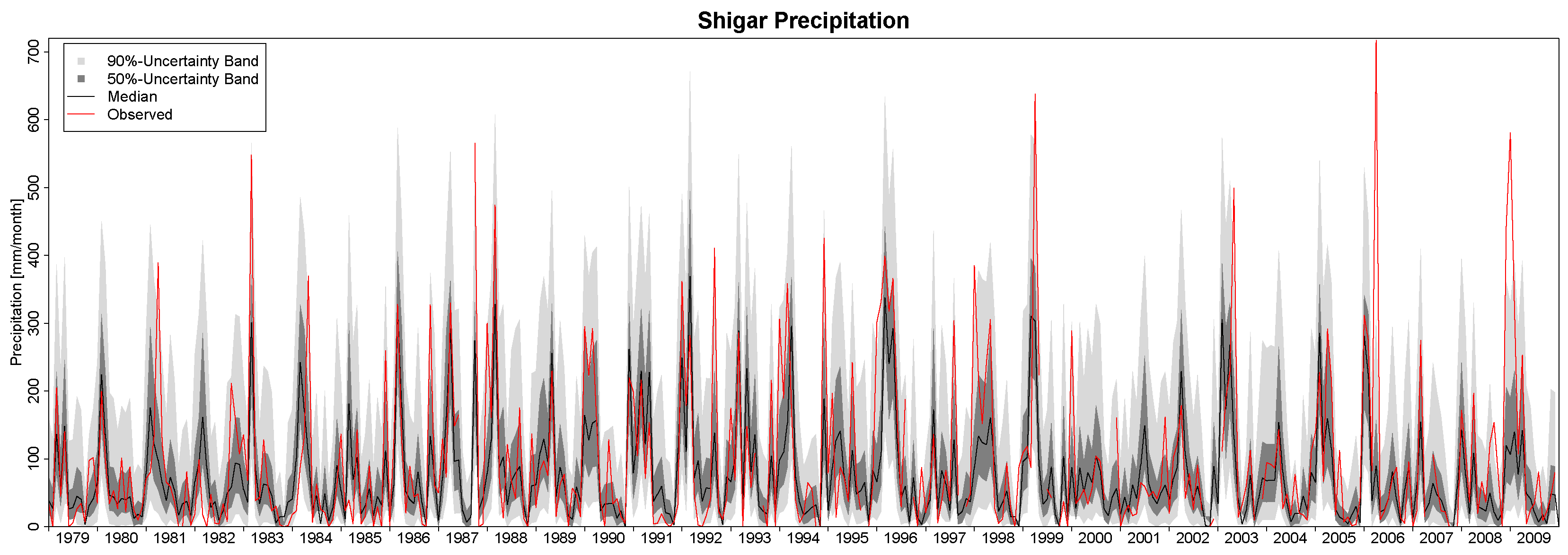
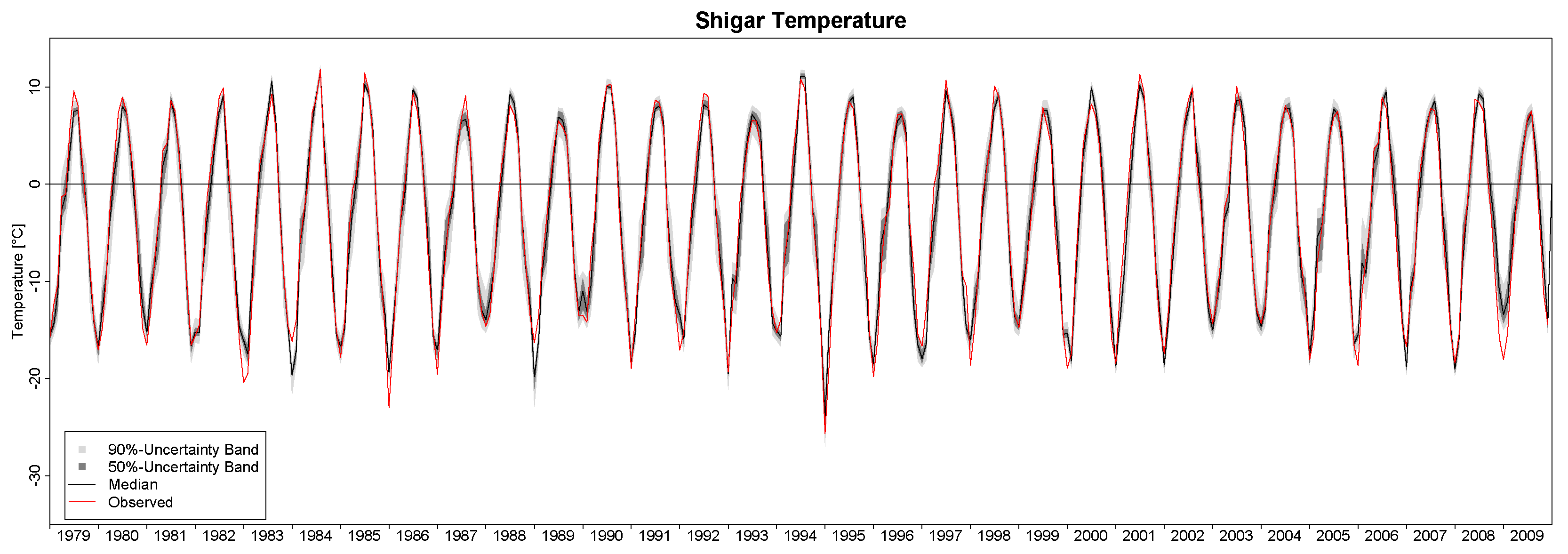
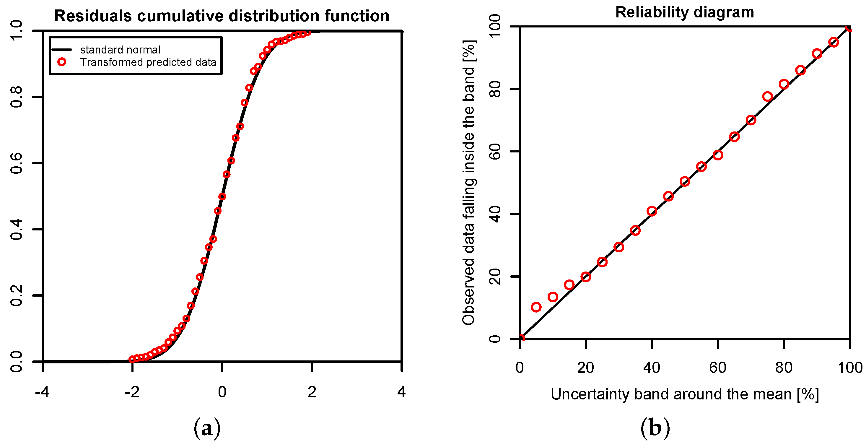
In this study, we have applied the Bayesian paradigm for prediction to quantitatively assess the uncertainty of precipitation and temperature estimates in a poorly-gauged basin in Central Karakoram by a six-member ensemble of independent reanalysis outputs. To this end, the Bayesian Model-Conditional Processor (MCP) has been used to estimate the predictive uncertainty for two meteorological variables required in regional hydro-glaciological mass balance analysis. The processor has been conditioned on monthly precipitation and temperature observations at a single observing station located in the proximity of the basin, which were mapped to the elevation of the basin centroid via an empirical scaling relationship and the adiabatic lapse rate. The reanalysis predictions were elaborated with the processor to remove the bias due to the different reference elevations of the atmospheric model vs. basin centroid elevation and to weight them according to their correlation with observations. The results show that the combination of the model predictions in the processing leads to a considerable reduction of the predictive uncertainty and an improved signal-to-noise ratio. The gain is more pronounced for temperature than for precipitation. Already, the use of a single reanalysis model, conditioned on observations, leads to noticeable improvements, but maximum benefit is obtained by the Bayesian combination of multiple independent predictions, six in our case. It needs to be emphasized that the combined result is only as good as the conditioning observations. Nevertheless, the obtained mean annual precipitation values summarized in Table 5 allow for a meaningful closure of the water balance. The continuous series of mean monthly precipitation and temperature and their variance can be used for specifying the uncertainty of atmospheric forcing in regional hydrological mass balance studies.

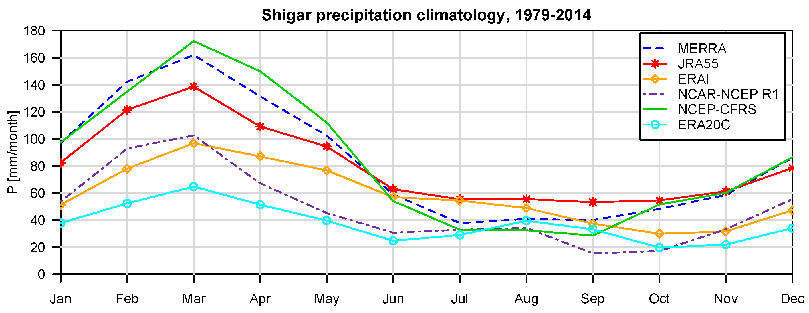
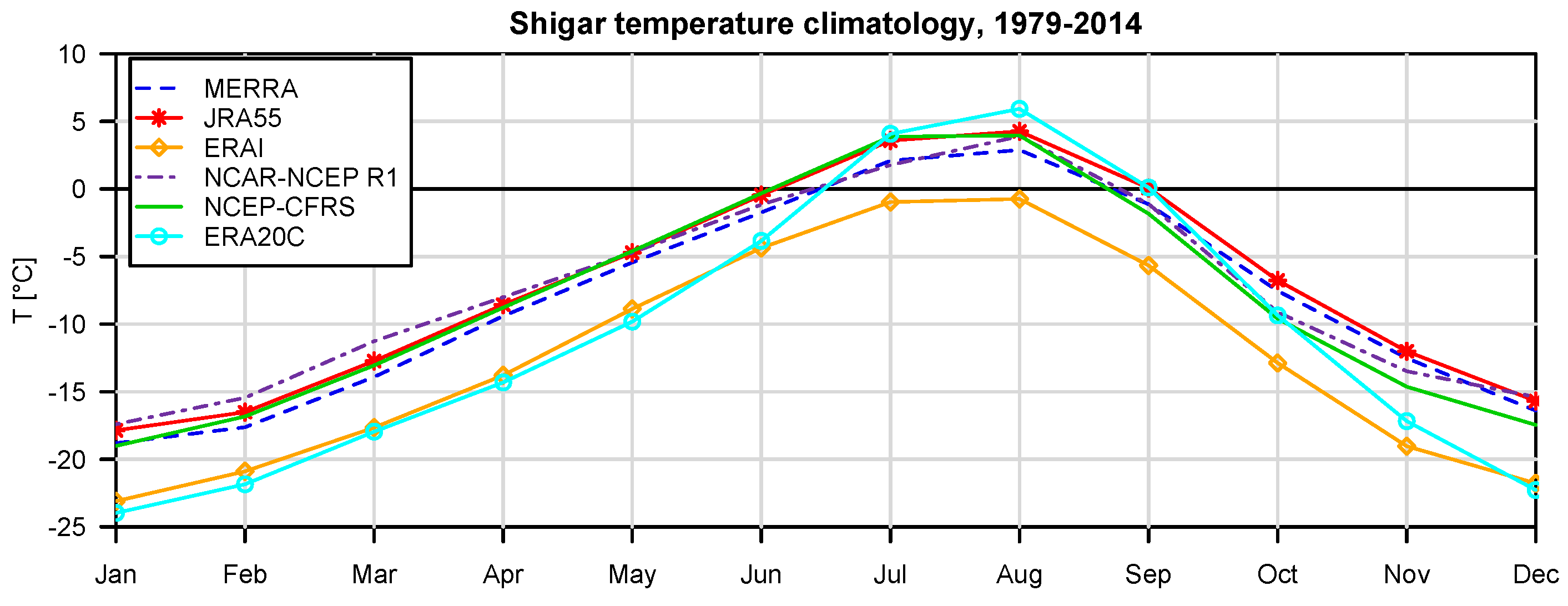
For the specific study region, which is characterized by extreme topographic relief and temperature excursions, there is a considerable difference in predictive capability between individual reanalysis products; JRA55 and NCEP-CFSR perform best for temperature, while JRA55 and ERA INTERIM outperform for precipitation. In general, the predictions of monthly precipitation, a diagnostic variable, are much more uncertain than those of temperature, a prognostic quantity. The study suggests that the use of reanalysis data for precipitation with sub-monthly resolution is to be considered as not adequate for hydrological studies in the region of interest. Future improvement of the sub-grid cloud and precipitation schemes in the atmospheric models are necessary for these products to become useful for applications with sub-monthly temporal resolution. The MCP also provides a solid conceptual basis for probabilistic reconstruction of missing observations and delivers the least uncertain atmospheric forcing data for poorly-gauged basins from atmospheric reanalysis data given conditioning observations.

References

1. Bolch, T.; Kulkarni, A.; Kääb, A.; Huggel, C.; Paul, F.; Cogley, J.G.; Frey, H.; Kargel, J.S.; Fujita, K.; Scheel, M.; et al. The state and fate of Himalayan glaciers. Science 2012, 336, 310–314. [Google Scholar] [CrossRef] [PubMed] [Green Version]
2. Cogley, G.C. Climate science: Himalayan glaciers in the balance. Nature 2012, 488, 468–469. [Google Scholar] [CrossRef] [PubMed]
3. Archer, D.R.; Fowler, H.J. Spatial and temporal variations in precipitation in the Upper Indus Basin, global teleconnections and hydrological implications. Hydrol. Earth Syst. Sci. 2004, 8, 47–61. [Google Scholar] [CrossRef]
4. Fowler, H.J.; Archer, D.R. Conflicting Signals of Climatic Change in the Upper Indus Basin. J. Clim. 2006, 19, 4276–4293. [Google Scholar] [CrossRef]
5. Forsythe, N.; Kilsby, C.G.; Fowler, H.J.; Archer, D.R. Assessment of runoff sensitivity in the Upper Indus Basin to interannual climate variability and potential change using MODIS satellite data products. Mt. Res. Dev. 2012, 32, 16–29. [Google Scholar] [CrossRef]
6. Mukhopadhyay, B.; Khan, A. A quantitative assessment of the genetic sources of the hydrologic flow regimes in Upper Indus Basin and its significance in a changing climate. J. Hydrol. 2014, 509, 549–572. [Google Scholar] [CrossRef]
7. Mukhopadhyay, B.; Khan, A. Rising river flows and glacial mass balance in central Karakoram. J. Hydrol. 2014, 513, 192–203. [Google Scholar] [CrossRef]
8. Mukhopadhyay, B.; Khan, A. Are-evaluation of the snowmelt and glacial melt in river flows within the Upper Indus Basin and its significance in a changing climate. J. Hydrol. 2015, 527, 119–132. [Google Scholar] [CrossRef]
9. Hewitt, K. The Karakoram Anomaly? Glacier Expansion and the Elevation Effect, Karakoram Himalaya. Mt. Res. Dev. 2005, 25, 332–340. [Google Scholar] [CrossRef]
10. Hewitt, K. Tributary glacial surges: An exceptional concentration at Panmah Glacier, Karakoram, Himalaya. J. Glaciol. 2007, 53, 181–188. [Google Scholar] [CrossRef]
11. Kehrwald, M.N.; Thompson, L.G.; Tandong, Y.; Mosley-Thompson, E.; Schotterer, U.; Alfimov, V.; Beer, J.; Eikenberg, J.; Davis, M.E. Mass loss on Himalayan glacier endangers water resources. Geophys. Res. Lett. 2008, 35, L22503. [Google Scholar] [CrossRef]
12. Gardelle, J.; Berthier, E.; Arnaud, Y. Slight mass gain of Karakoram glaciers in the early 21st century. Nat. Geosci. 2012, 5, 322–325. [Google Scholar] [CrossRef]
13. Kääb, A.; Berthier, E.; Nuth, C.; Gardelle, J.; Arnaud, Y. Contrasting patterns of early twenty-first-century glacier mass change in the Himalayas. Nature 2012, 488, 495–498. [Google Scholar] [CrossRef] [PubMed]
14. Jacob, T.; Wahr, J.; Pfeffer, W.T.; Swenson, S. Recent contributions of glaciers and ice caps to sea level rise. Nature 2012, 482, 514–518. [Google Scholar] [CrossRef] [PubMed]
15. Bhutyani, M.R. Mass-balance studies on Siachen Glacier in the Nubra valley, Karakoram Himalaya, India. Ann. Glaciol. 1999, 45, 112–118. [Google Scholar]
16. Harris, I.; Jones, P.D.; Osborn, T.J.; Lister, D.H. Updated high-resolution grids of monthly climatic observations—The CRU TS3.10 Dataset. Int. J. Climatol. 2013, 34, 623–642. [Google Scholar] [CrossRef] [Green Version]
17. Schneider, U.; Becker, A.; Finger, P.; Meyer-Christoffer, A.; Ziese, M.; Rudolf, B. GPCC’s new land surface precipitation climatology based on quality-controlled in situ data and its role in quantifying the global water cycle. Theor. Appl. Climatol. 2013, 115, 15–40. [Google Scholar] [CrossRef]
18. Immerzeel, W.W.; Pellicciotti, F.; Shrestha, A.B. Glaciers as a proxy to quantify the spatial distribution of precipitation in the Hunza Basin. Mt. Res. Dev. 2012, 32, 3–38. [Google Scholar] [CrossRef]
19. Reggiani, P.; Rientjes, T.H.M. A reflection on the long-term water balance of the Upper Indus Basin. Hydrol. Res. 2015, 3, 446–462. [Google Scholar] [CrossRef]
20. Condom, T.; Rau, P.; Espinoza, J.C. Correction of TRMM 3B43 monthly precipitation data over the mountainous areas of Peru during the period 1998–2007. Hydrol. Process. 2011, 25, 1924–1933. [Google Scholar] [CrossRef]
21. Ward, E.; Buytaert, W.; Peaver, L.; Wheater, H. Evaluation of precipitation products over complex mountainous terrain: A water resources perspective. Adv. Water Resour. 2011, 34, 1222–1231. [Google Scholar] [CrossRef]
22. Dee, D.P.; Balmaseda, M.; Balsamo, G.; Engelen, R.; Simmons, A.J.; Thepaut, J.N. Toward a Consistent Reanalysis of the Climate System. Bull. Am. Meteorol. Soc. 2014, 95, 1235–1248. [Google Scholar] [CrossRef]
23. Blum, J.; Le Dimet, F.X.; Navon, I.M. Data assimilation for geophysical fluids. In Computational Methods for the Atmosphere and the Oceans, Handbook of Numerical Analysis; Ciarlet, P.G., Temam, R., Tribbia, J., Eds.; Elsevier Science: Amsterdam, The Netherlands, 2008; Volume 14, pp. 385–442. [Google Scholar]
24. Kalnay, E.; Li, H.; Miyoshi, T.; Yang, S.C.; Ballabrera-Poy, J. 4-D-Var or ensemble Kalman filter? Tellus A 2007, 59, 758–773. [Google Scholar] [CrossRef]
25. Evensen, G. The ensemble Kalman filter: Theoretical formulation and practical implementation. Ocean Dyn. 2007, 50, 343–367. [Google Scholar] [CrossRef]
26. Glahn, H.R.; Lowry, D.A. The use of model output statistics (MOS) in objective weather forecasting. J. Appl. Meteorol. 1972, 11, 1203–1211. [Google Scholar] [CrossRef]
27. Wilks, D.S. Statistical Methods in the Atmospheric Sciences: An Introduction; Academic Press: London, UK, 1995; p. 467. [Google Scholar]
28. Coccia, G.; Siemann, A.L.; Pan, M.; Wood, E.F. Creating consistent datasets by combining remotely-sensed data and land surface model estimates through Bayesian uncertainty post-processing: The case of Land Surface Temperature from HIRS. Remote Sens. Environ. 2015, 170, 290–305. [Google Scholar] [CrossRef]
29. Kistler, R.; Kalnay, E.; Collins, W.; Saha, S.; White, G.; Woollen, J.; Chelliah, M.; Ebisuzaki, W.; Kanamitsu, M.; Kousky, V.; et al. The NCEP-NCAR 50-Year Reanalysis: Monthly Means CD-ROM and Documentation. Bull. Am. Meteorol. Soc. 2001, 82, 247–267. [Google Scholar] [CrossRef]
30. Todini, E. A model conditional processor to assess predictive uncertainty in flood forecasting. Int. J. River Basin Manag. 2008, 36, 3265–3277. [Google Scholar] [CrossRef]
31. Coccia, G.; Todini, E. Recent developments in predictive uncertainty assessment based on the Model Conditional Processor approach. Hydrol. Earth Syst. Sci. 2011, 15, 3253–3274. [Google Scholar] [CrossRef]
32. Wilby, R.L.; Wigley, T.M.L. Downscaling general circulation model output: A review of methods and limitations. Prog. Phys. Geogr. 1997, 21, 530–548. [Google Scholar] [CrossRef]
33. Immerzeel, W.W.; Wanders, N.; Lutz, A.F.; Shea, J.M.; Bierkens, M.F.P. Reconciling high-altitude precipitation in the upper Indus basin with glacier mass balances and runoff. Hydrol. Earth Syst. Sci. 2015, 19, 4673–4687. [Google Scholar] [CrossRef]
34. Yatagai, A.; Yasutomi, N.; Hamada, A.; Kitoh, A.; Kamiguchi, K.; Arakawa, O. APHRODITE: Constructing a long-term daily gridded precipitation dataset for Asia based on a dense network of rain gauges. Geophys. Res. Abstr. 2012, 14, 1401–1415. [Google Scholar] [CrossRef]
35. Pfeffer, W.T.; Arendt, A.; Bliss, A.; Bolch, T.; Cogley, J.; Gardner, A.; Hagen, J.; Hock, R.; Kaser, G.; Kienholz, C.; et al. The Randolph Glacier Inventory: A globally complete inventory of glaciers. J. Glaciol. 2014, 60, 537–552. [Google Scholar] [CrossRef] [Green Version]
36. Singh, P.; Ramashastri, K.S.; Kumar, N. Topographic influences on precipitation distribution in different ranges of the western Himalayas. Nord. Hydrol. 1995, 26, 259–284. [Google Scholar]
37. Palazzi, E.; von Hardenberg, J.; Provenzale, A. Precipitation in the Hindu-Kush Karakoram-Himalaya: Observations and future scenarios. J. Geophys. Res. Atmos. 2013, 118, 85–100. [Google Scholar] [CrossRef]
38. Young, J.G.; Hewitt, K. Hydrology Research in the Upper Indus Basin, Karakoram, Himalaya, Pakistan; IAHS Publ. No. 190; IAHS Press: Wallingford, UK, 1990; pp. 139–152. [Google Scholar]
39. Wake, C.P. Glaciochemical investigations as a tool for determining the spatial and seasonal variation of snow accumulation in the central Karakoram, northern Pakistan. Ann. Glaciol. 1989, 13, 279–248. [Google Scholar]
40. Hewitt, K. Glacier change, concentration, and elevation effects in the Karakoram Himalaya, Upper Inreus Basin. Mt. Res. Dev. 2011, 31, 188–200. [Google Scholar] [CrossRef]
41. Dreyer, N.; Nikolayeva, G.; Tsigelnaya, T. Maps of stream flow resources of some high mountain areas in Asia and North America. Int. Assoc. Hydrol. Sci. 1982, 138, 203–208. [Google Scholar]
42. Hewitt, K.; Wake, C.P.; Young, G.J.; David, C. Hydrological investigations at Biafo Glacier, Karakoram Range, Himalaya; an important source of water for the Indus River. Ann. Glaciol. 2011, 13, 103–108. [Google Scholar]
43. Douie, J. The Panjab, North-West frontier province, and Kashmir. In Provincial Geographies of India; Holland, T., Ed.; Cambridge University Press: Cambridge, UK, 1916. [Google Scholar]
44. Kaser, G.; Grosshauser, M.; Marzeion, B. Contribution of glaciers to water availability in different climate regimes. Proc. Natl. Acad. Sci. USA 2010, 107, 20223–20227. [Google Scholar] [CrossRef] [PubMed]
45. Bookhagen, B.; Burbank, D.W. Toward a complete Himalayan hydrological budget: Spatiotemporal distribution of snowmelt and rainfall and their impact on river discharge. J. Geophys. Res. 2010, 115, F03019. [Google Scholar] [CrossRef]
46. Immerzeel, W.W.; Droogers, P.; de Jong, S.M.; Bierkens, M.F.P. Large-scale monitoring of snow cover and runoff simulation in Himalayan river basins using remote sensing. Remote Sens. Environ. 2009, 113, 40–49. [Google Scholar] [CrossRef]
47. Forsythe, N.; Fowler, H.J.; Kilsby, C.G.; Archer, D.R. Opportunities from Remote Sensing for Supporting Water Resources Management in Village/Valley Scale Catchments in the Upper Indus Basin. Water Resour. Manag 2011, 26, 245–251. [Google Scholar] [CrossRef]
48. Krzysztofowicz, R. Bayesian theory of probabilistic forecasting via deterministic hydrologic model. Water Resour. Res. 1999, 35, 2739–2750. [Google Scholar] [CrossRef]
49. Krzysztofowicz, R.; Kelly, K.S. Hydrologic uncertainty processor for probabilistic river stage forecasting. Water Resour. Res. 2000, 35, 2739–2750. [Google Scholar] [CrossRef]
50. Raftery, A.E. Bayesian model selection in structural equation models. In Testing Structural Equation Models; Bollen, K.A., Long, J.S., Eds.; Sage: Newbury Park, CA, USA, 1993; pp. 163–180. [Google Scholar]
51. Raftery, A.E.; Gneiting, T.; Balabdaoui, F.; Polakowski, M. Using Bayesian model averaging to calibrate forecast ensembles. Mon. Weather Rev. 2005, 133, 1155–1174. [Google Scholar] [CrossRef]
52. Vrugt, J.A.; Robinson, B.A. Treatment of uncertainty using ensemble methods: Comparison of sequential data assimilation and Bayesian model averaging. Water Resour. Res. 2007, 43, W01411. [Google Scholar] [CrossRef]
53. Koenker, R. Quantile Regression. In Econometric Society Monographs; Cambridge University Press: New York, NY, USA, 2005. [Google Scholar]
54. Stickler, A.; Brönnimann, S.; Valente, M.A.; Bethke, J.; Sterin, A.; Jourdain, S.; Roucaute, E.; Vasquez, M.V.; Reyes, D.A.; Allan, R.; et al. ERA-CLIM: Historical Surface and Upper-Air Data for Future Reanalyses. Bull. Am. Meteorol. Soc. 2010, 95, 1419–1430. [Google Scholar] [CrossRef]
55. Kobayashi, S.; Ota, Y.; Harada, Y.; Ebita, A.; Moriya, M.; Onoda, H.; Onogi, K.; Kamahori, H.; Kobayashi, C.; Endo, H.; et al. The JRA-55 Reanalysis: General Specifications and Basic Characteristics. J. Met. Soc. Jpn. 2015, 93, 5–48. [Google Scholar] [CrossRef]
56. Saha, S.; Moorthi, S.; Pan, H.L.; Wu, X.; Wang, J.; Nadiga, S.; Tripp, P.; Kistler, R.; Woollen, J.; Behringer, D.; et al. The NCEP Climate Forecast System Reanalysis. Bull. Am. Meteorol. Soc. 2010, 91, 1015–1057. [Google Scholar] [CrossRef]
57. Rienecker, M.M.; Suarez, M.J.; Gelaro, R.; Todling, R.; Bacmeister, J.; Liu, E.; Bosilovich, M.G.; Schubert, S.D.; Takacs, L.; Kim, G.K.; et al. MERRA: NASA’s Modern-Era Retrospective Analysis for Research and Applications. J. Clim. 2011, 24, 3624–3648. [Google Scholar] [CrossRef]
58. Cramer, T. Geländeklimatologische Studien im Bragottal, Karakorumgebirge, Pakistan; GEO Aktuell Forschungsarbeiten: Göttingen, Germany, 2000; Volume 3. (In German) [Google Scholar]
59. Kuhle, M. The maximum ice age glaciation between the Karakorum main ridge (K2) and the Tarim basin and its influence on global energy balance. J. Mt. Sci. 2005, 2, 5–22. [Google Scholar] [CrossRef]
60. Winiger, M.; Gumpert, M.; Yamout, H. Karakoram-Hindukush-Western Himalaya: Assessing high-altitude water resources. Hydrol. Process. 2005, 19, 2329–2338. [Google Scholar] [CrossRef]
61. Bocchiola, D.; Diolaiuti, G.; Soncini, A.; Mihalcea, C.; D’Agata, C.; Mayer, C.; Lambrecht, A.; Rosso, R.; Smiraglia, C. Prediction of future hydrological regimes in poorly gauged high altitude basins: The case study of the upper Indus, Pakistan. Hydrol. Earth Syst. Sci. 2011, 15, 2059–2075. [Google Scholar] [CrossRef]
62. Miehe, G.; Wininger, M.; Böhner, M.; Yili, Z. The climatic diagram map of High Asia. Erdkunde 2001, 55, 94–97. [Google Scholar] [CrossRef]
63. Tallis, G.M. The moment generating function of the truncated multi-normal distribution. J. R. Stat. Soc. 1961, 23, 223–229. [Google Scholar]
64. Todini, E. From HUP to MCP: Analogies and extended performances. J. Hydrol. 2012, 477, 32–43. [Google Scholar] [CrossRef]
65. Mardia, K.V.; Kent, J.T.; Bibby, J.M. Multivariate Analysis. Probability and Mathematical Statistics; Academic Press: London, UK, 1979. [Google Scholar]
Figure 1. The Upper Indus Basin area upstream of Tarbela reservoir and Shigar Basin as an excerpt. The blue triangles indicate stream gauging stations operated by the Pakistani Water and Power Development Authority (WAPDA), and the green bullets indicate meteorological stations operated by the Pakistani Meteorological Department (PMD), except the station at Leh, which is operated by the Indian Meteorological Department (IMD).
Water 08 00263 g001
Figure 2. Precipitation climatology derived from the six selected reanalysis products listed in Table 1 for Shigar Basin.
Water 08 00263 g002
Figure 3. Temperature climatology derived from the six selected reanalysis products listed in Table 1 for Shigar Basin. CFSR, Climate Forecast System Reanalysis.
Water 08 00263 g003
Figure 4. Double Mass curve analysis of Skardu vs. Sadpara (Deosai), Hushey, Shigar. The strong and sudden deviation from the bisection after a short recording period (>1000 mm/month accumulated precipitation) exposes the inconsistency of the short-term record stations with respect to Skardu.
Water 08 00263 g004
Figure 5. Transformed observed monthly precipitation data η against transformed predictions η ^ i for all six models. The dashed lines indicate the 90% credible interval, the continuous line the median. A two-piece truncated normal distribution has been fitted to all cases, except ERA Interim and ERA20, because of the heteroscedasticity of the dependence ( η , η i ).
Water 08 00263 g005
Figure 6. Transformed observed monthly mean temperature data η against transformed predictions η ^ i for all six models. The dashed lines indicate the 90% credible interval, the continuous line the median. The relation of the variables can be modeled with a single multi-normal distribution, as the dependence ( η , η ^ i ) can be approximated as homoscedastic.
Water 08 00263 g006
Figure 7. Monthly mean observed and reconstructed precipitation values and their uncertainty for Shigar Basin, 1979–2009. Altitude-adjusted observations are indicated with a solid red line and the median of predictions with a solid black line. Shadowed areas indicate the 50% and 90% credible intervals.
Water 08 00263 g007
Figure 8. Monthly mean observed temperature for Shigar Basin, 1979–2009. Altitude-adjusted observations are indicated with a solid red line and the median of predictions with a solid black line. Shadowed areas indicate the 50% and 90% credible intervals.
Water 08 00263 g008
Figure 9. (a) verification of the normality of residuals for precipitation against the distribution N(0,0.48), uncensored data, all six models, 1979–2009; (b): reliability diagram with the percentage of observations that fall inside the uncertainty band at various 10% probability intervals. The continuous line represents perfect behavior.
Water 08 00263 g009
Figure 10. (a): verification of the normality of residuals for temperature against the distribution N(0,0.06), uncensored data, all six models, 1979–2009; (b): reliability diagram with the percentage of observations that fall inside the uncertainty band at various 10% probability intervals. The continuous line represents perfect behavior.
Water 08 00263 g010