Article

A Long-Term Study of Ecological Impacts of River Channelization on the Population of an Endangered Fish: Lessons Learned for Assessment and Restoration

by
James H. Roberts
1,
Gregory B. Anderson
2,† and
Paul L. Angermeier
3,*
1
Department of Biology, Georgia Southern University, Statesboro, GA 30458, USA
2
Department of Fish and Wildlife Conservation, Virginia Polytechnic Institute and State University, Blacksburg, VA 20461, USA
3
U.S. Geological Survey, Virginia Cooperative Fish and Wildlife Research Unit, Blacksburg, VA 20461, USA
*
Author to whom correspondence should be addressed.
Present address: Environmental Solutions & Innovations, Inc., Cincinnati, OH 45232, USA
Water 2016, 8(6), 240; https://doi.org/10.3390/w8060240
Submission received: 2 February 2016 / Revised: 17 April 2016 / Accepted: 19 April 2016 / Published: 3 June 2016

Abstract

:
Projects to assess environmental impact or restoration success in rivers focus on project-specific questions but can also provide valuable insights for future projects. Both restoration actions and impact assessments can become “adaptive” by using the knowledge gained from long-term monitoring and analysis to revise the actions, monitoring, conceptual model, or interpretation of findings so that subsequent actions or assessments are better informed. Assessments of impact or restoration success are especially challenging when the indicators of interest are imperiled species and/or the impacts being addressed are complex. From 1997 to 2015, we worked closely with two federal agencies to monitor habitat availability for and population density of Roanoke logperch (Percina rex), an endangered fish, in a 24-km-long segment of the upper Roanoke River, VA. We primarily used a Before-After-Control-Impact analytical framework to assess potential impacts of a river channelization project on the P. rex population. In this paper, we summarize how our extensive monitoring facilitated the evolution of our (a) conceptual understanding of the ecosystem and fish population dynamics; (b) choices of ecological indicators and analytical tools; and (c) conclusions regarding the magnitude, mechanisms, and significance of observed impacts. Our experience with this case study taught us important lessons about how to adaptively develop and conduct a monitoring program, which we believe are broadly applicable to assessments of environmental impact and restoration success in other rivers. In particular, we learned that (a) pre-treatment planning can enhance monitoring effectiveness, help avoid unforeseen pitfalls, and lead to more robust conclusions; (b) developing adaptable conceptual and analytical models early was crucial to organizing our knowledge, guiding our study design, and analyzing our data; (c) catchment-wide processes that we did not monitor, or initially consider, had profound implications for interpreting our findings; and (d) using multiple analytical frameworks, with varying assumptions, led to clearer interpretation of findings than the use of a single framework alone. Broader integration of these guiding principles into monitoring studies, though potentially challenging, could lead to more scientifically defensible assessments of project effects.

1. Introduction

Globally, riverine ecosystems are extensively modified, directly and indirectly, by anthropogenic activities. Human demands on rivers are growing, leading to large and growing threats to ecosystem services provided by rivers as well as to their biodiversity, including fishes [1,2,3,4]. Efforts to quantify and mitigate adverse anthropogenic impacts commonly include projects designed to assess impact or to restore valued riverine conditions. These efforts inform project-specific management questions but can also, if properly designed and analyzed, provide valuable insights to enhance the efficacy of future assessment and management actions. In this paper, we draw from previous syntheses of river restoration [5,6,7,8,9,10,11,12,13,14] to show how the proper application of scientific approaches can lead to more effective and informative assessment and restoration efforts.
Scientific approaches to assessing environmental impacts on rivers and restoring rivers share important similarities. Accurately assessing impacts and designing effective restorations both require attention to the key factors, processes, and mechanisms that regulate the system and/or components of interest. This mechanistic knowledge, drawn from ecological expertise and theory, is perhaps most useful when synthesized into a conceptual model of how key factors and processes produce ecological outcomes. Often, assessments are focused on gauging effects of a project on populations of aquatic organisms, because aquatic biota provide information about ecosystem condition [15], are socioeconomically valuable, and may be legally protected. For projects involving populations, knowledge of species’ life history, habitat use, and dispersal is crucial [16]. Assessing impact magnitude or restoration success both require teasing environmental signals from the background noise of the spatiotemporal variation exhibited by real ecosystems [17]. The scope (spatial extent and temporal duration) of habitat use by focal species must be acknowledged so all relevant life stages are considered [18,19]. Detecting relevant signals requires paying attention to the spatiotemporal design of monitoring protocols and the selection of ecological indicators to be monitored. Interpretation of monitoring results requires a priori thresholds of acceptability (for impacts) or success (for restoration). Whether a system crosses such thresholds can be treated statistically as testable hypotheses, which may be derived from the conceptual model. Similarities between impact and restoration assessment suggest that lessons learned from one field could inform the other.

1.1. Learning by Doing

Restoration actions and impact assessments can become “adaptive” by using the knowledge gained from monitoring and analysis to revise the actions, monitoring, conceptual model, or interpretation so that subsequent actions or assessments are better informed and more likely to be effective. Adaptive management (AM) has long been promoted as a scientifically sound approach to natural resource management [20,21,22]. AM is especially well suited for systems characterized by substantial uncertainty because AM emphasizes “learning by doing”, where learning is not achieved by simple trial and error [6] but is founded on careful, hypothesis-driven monitoring and treating management actions as experiments. Indicators to monitor are selected to match stakeholder values, project objectives, and budgets [23]. Thus, AM is widely touted as the preferred approach to river restoration [6,23,24,25], and by extension, is applicable to long-term impact assessments for aquatic populations [26,27,28]. In short, an AM approach allows a management or assessment choice to be made, based on best available knowledge, then allows the choice to be revisited as more is learned about the operation and responses of an ecosystem. The number of AM steps or phases recognized varies among AM advocates but below we discuss 12 main steps germane to impact and restoration monitoring in general and to our case study in particular (Table 1).
Although AM is strongly promoted by scientists, its implementation by those performing restoration and assessment is often lackluster, a pattern that limits effectiveness, project-specific learning, and development of broadly applicable ecological knowledge. Common limitations to effective river restoration include weak knowledge of watershed-scale processes, institutional structures poorly suited to large-scale management, and severe financial constraints [25]; in our experience, these limitations are shared by impact assessments. Monitoring, evaluation, and reporting are crucial components of the AM approach, which enable practitioners to assess the significance of measured impacts, determine the success of restoration actions, and facilitate ecological learning. Even so, these steps are commonly compromised in or omitted from restoration programs [5,6,7,9]. Similarly, many restoration projects operate under weak conceptual models and/or inappropriate spatiotemporal scales [7]. Similar shortfalls in the AM approach are common in impact assessments [26,27,28].

1.2. Challenges of Assessing Impacts on Populations

Assessments of environmental impact or restoration success that address responses of wild populations are more complicated than assessments that address only physicochemical responses [25]. Populations respond to broad arrays of physical, chemical, and biological factors—at multiple spatiotemporal scales—that interact in complex ways over the course of life history. Large-scale, long-term dynamics of ecosystems are especially likely to be poorly understood [29]. Further, because population responses integrate environmental effects on behavior, growth, survival, and reproduction of many individuals, timelines for population responses may include time lags and other forms of temporal variation. For example, fish populations may exhibit region-wide boom-bust patterns that reflect annual variation in recruitment [30]. High inter-annual variation in fish abundance can preclude detection of impacts and may not provide feedback sensitive or rapid enough to prevent impacts from causing unacceptable harm, especially for rare taxa [31]. Even if an impact on a population is detected statistically, determining what impact-level is significant in the context of population persistence is a major and difficult problem [32]. Finally, for imperiled species, crucial knowledge on life-history, distribution, and population dynamics may not exist [29,33], thereby hampering the design of assessment protocols and interpretation of findings.
Availability of suitable habitat is essential for population persistence and often drives population dynamics, but does not necessarily limit populations [34]. Any assessment of population response must include an assessment of habitat suitability, even if potential changes in non-habitat factors are the main impetus for the assessment. Assessments of habitat suitability can take many forms and include multiple spatial scales [35,36], which can complement assessments of other factors of interest to produce an overall assessment of impact or restoration success. River projects commonly focus on habitat suitability. Habitat loss is a top impetus for river restoration [13] and in-stream habitat improvement is a top restoration goal [7,9]. Even so, relations between suitable habitat and population abundance are complex, and the two metrics may be weakly correlated. For example, river rehabilitation projects in the United Kingdom typically improved habitat and flow but did not benefit macroinvertebrates and fishes [37]. In a review of studies of reach-scale responses of invertebrates to restoration, Palmer et al. [11] found that most projects did enhance habitat quality but few showed significant increases in taxa richness (see also [38]). Further, most experimental studies in healthy streams showed no positive relationship between habitat complexity and invertebrate diversity [11]. Weak correlations between habitat suitability and population responses may reflect mismatches in spatiotemporal scales between habitat assessment or restoration and the processes that regulate populations [39,40].

1.3. Challenges of Assessing Biological Effects of Fine Sediment

Excess fine sediment is pervasive in streams and rivers draining intensively altered landscapes and is a top cause of stream impairment [41] and fish imperilment [42]. Excess fine sediment has profound direct and indirect effects on lotic ecosystem structure and function, including effects on water and habitat quality and food webs [43,44]. Fishes can be affected by sediment via pathways of individuals’ physiology, behavior, growth, survival, or reproduction, and via population dynamics [45,46,47]. However, quantifying impacts of excess sediment on populations in rivers is exceedingly difficult because of (a) multiple interacting pathways; (b) high temporal variation in sediment loading, transport, and deposition, which may feature episodic events and time lags [48,49]; and (c) potential mismatches between the spatiotemporal scales of sediment dynamics versus population dynamics. Thus, measurable impacts on a particular population may not manifest as monotonic or consistent signals in the indicators selected for monitoring. For similar reasons, it may be difficult to detect intended biological responses to management actions that aim to control sediment-loading or restore more natural sediment dynamics.
Urban rivers are frequently the subject of impact- or restoration-based monitoring [50,51]. Yet, urban rivers present special problems for assessing impacts of excess sediment or restoring semi-natural sediment dynamics. Urbanization imposes a long list of impacts on river ecosystems [52,53,54,55], including excess fine sediment from watersheds and stream channels. Urban rivers are problematic in the context of assessing restoration outcomes and specific environmental impacts because of the many unknown but potentially confounding impacts, including alterations in hydrology, temperature regime, sediment and contaminant loads, and channel morphology [10]. Distinguishing effects of elevated fine sediment from effects of other alterations in urban rivers is likely to require a carefully designed study and long timeframe.

1.4. Challenges of Assessing Impacts on Endangered Species

Imperiled species protection in the U.S. is accomplished largely by the Endangered Species Act (ESA) of 1973, as well as by state-level analogs. Analogous legal frameworks (e.g., the Species at Risk Act in Canada, the Bern Convention in Europe) are present in many other nations. The ESA prohibits “take” (i.e., harassing, harming, pursuing, hunting, shooting, wounding, killing, trapping, capturing, or collecting) of listed species. Any human activity that might cause take is subject to review by the U.S. Fish and Wildlife Service (USFWS), who administers the ESA for inland species. However, the ESA provides for compromise between species protection and human activities by allowing “incidental take” (i.e., take ancillary to conducting an otherwise lawful activity). The USFWS may exempt incidental take of listed species from the Section 9 prohibitions of the ESA through an incidental take statement (ITS) via a Biological Opinion (BO) for federal actions or via an Incidental Take Permit for actions of private parties (Sections 7 and 10 of the ESA). The incidental take permit or statement will specify the amount or extent of anticipated take and the measures required to minimize, mitigate, and monitor take.
Accurate assessments of incidental take require scientific input during all five stages of development, including (1) assessment of current status of species; (2) estimation of the anticipated amount of incidental take; (3) evaluation of how estimated take will affect species; (4) proposed measures to minimize or mitigate for take; and (5) proposed protocols for monitoring amounts of take [33]. However, all stages may include considerable uncertainty, and uncertainty in early stages (e.g., assessing species status) becomes compounded in later stages (e.g., evaluating effects of take). Uncertainty is often exacerbated by sparse knowledge of endangered species, many of which are rare or obscure [29,33]. Rigorous experimental study and AM of such species may be infeasible because populations and habitat cannot be replicated and because ethical and legal issues constrain the creation and destruction of suitable habitat [28]. Mathematical models can be useful for simulating population dynamics, but lack of detailed demographic data may make these models difficult to parameterize. For example, Harding et al. [33] evaluated the use of science in a sample of take permits within approved Habitat Conservation Plans. They found that planners generally incorporated available science into plans, but that data on life-history, population trends, and effectiveness of mitigation often did not exist. As a result, take was often unquantifiable, and monitoring measures were insufficient to assess take.

1.5. Aim of This Paper

The review above identifies five issues potentially central to monitoring ecological effects of impacts or restoration: (1) the need for a rigorous, well-conceived process; (2) the importance of AM; (3) the challenge of quantifying population-level responses; (4) the challenges of detecting biological responses to changes in the delivery of fine sediment; and (5) the challenges particular to monitoring threatened and endangered species. All these issues are germane to our case study (below) on assessing impacts of river channelization for Roanoke logperch (Percina rex; Jordan and Evermann 1889). We monitored P. rex and their habitat primarily to estimate incidental take and assess population-level impacts, even though basic knowledge about population dynamics of the species was initially sparse and uncertainty about how observed take related to these dynamics was high. Even so, our long-term (19 years) monitoring enabled us to learn valuable lessons that advanced our knowledge of P. rex ecology and made management for the species more cost-effective [56,57,58].
In this paper, we summarize how our extensive spatiotemporal monitoring to assess potential impacts of a river channelization project facilitated evolution (via learning) of our (a) conceptual understanding of how key ecological factors regulate the population dynamics of an endangered fish; (b) choices of ecological indicators and analytical tools; (c) understanding of the appropriate temporal and spatial scales necessary to detect population changes; and (d) conclusions regarding the magnitude, mechanisms, and biological significance of observed impact. We conclude with selected lessons generally applicable to assessing environmental impacts and restoration in other rivers.

2. Case Study: The Roanoke River Flood Reduction Project

2.1. Background

2.1.1. Study Species

Percina rex is a benthic darter (Actinopterygii: Percidae) endemic to streams in the Roanoke and Chowan river basins of Virginia and North Carolina. Its habitat needs and life-history are similar to other stream-dwelling members of the diverse genus Percina. During April–October, adult P. rex typically occupy swift, 30–100-cm-deep microhabitats within riffle-runs, where they forage for invertebrate prey under substrate particles they flip over with their conical snouts [58,59]. Spawning occurs in May-June over loosely embedded gravel in deep runs. Eggs and milt are broadcast over the substrate, where they sink into interstices. No parental care is provided. Young subsequently emerge and drift into backwaters and pool margins, where they forage in mixed-species shoals [58,60]. Like adults, juveniles prefer microhabitats with low silt cover and embeddedness, presumably because these patches offer better feeding efficiency. When they reach approximately 100 mm total length (TL), typically corresponding to age 1, P. rex begin transitioning into the swift mesohabitats occupied by adults. Maturity is reached by age 2 or 3. The species grows to a maximum length of 165 mm TL and a maximum age of approximately 7 years [59,61].
Reliance on unembedded substrate for feeding and reproduction predisposes P. rex to be vulnerable to excess silt deposition. Agricultural, silvicultural, and urbanization activities over the past 250 years likely dramatically increased silt transport and deposition in the Roanoke and Chowan basins [62]. It is hypothesized that the present distribution of P. rex, which comprises seven small, isolated populations, reflects the relicts of what was once a much larger, more continuous distribution [62,63]. Due to this presumed range reduction, and ongoing threats from continued land-use conversion, the species was listed as “endangered” in 1989, pursuant to the ESA. Recovery strategies for the species emphasize (a) reducing chemical pollution and spills; (b) removing barriers to movement; (c) establishing new populations; and particularly (d) reducing sediment loading into streams harboring the species [63]. A recent population viability analysis for the species indicated that both acute disturbances (e.g., pollution events) and chronic reductions in population growth rate and carrying capacity (e.g., due to habitat embeddedness) are important drivers of population size and extinction probability [64].

2.1.2. Study Area

The upper Roanoke River subbasin (U.S. Geological Survey (USGS) Hydrologic Unit Code 03010101) is a 5675-km2 watershed within the Valley and Ridge and Blue Ridge physiographic provinces of southwestern Virginia. This subbasin hosts approximately 374,850 people, a variety of water and land uses, and a fish fauna that is one of the most diverse of the Atlantic slope drainages of North America [62]. Upstream portions of the watershed drain predominantly forest and farmland, whereas the downstream third drains urbanized areas of Salem, Roanoke, and Vinton, Virginia. The study area comprised a 24-km-long, unregulated segment of the mainstem Roanoke River, including a 9-km-long control reach (reach C) and an adjacent downstream 15-km-long impact reach (reach I) that was the focus of flood-control construction activities (see below). The largest tributary in the study area, Mason Creek, enters the Roanoke River at the boundary of the two study reaches, but P. rex is not presently known to occupy this stream [63], so we presume that the creek had no influence on study findings. Stream gradient in the study area is 1.8 m·km−1 and typical wetted width during base flow ranges from 25 to 50 m. Habitat diversity is high, including riffle, run, and pool mesohabitats. Across mesohabitats, substrate consists primarily of shale, limestone, and dolomite gravel, rubble, and bedrock, with significant silt deposition occurring in pools and slow runs. At the downstream end of the study area, stream temperature ranges from 0 to 28 °C annually, and mean daily discharge ranges from 3.6 to 22.7 m3·s−1 annually [65].
Percina rex are continuously distributed among and relatively abundant within riffle-run mesohabitats in the study reach, which is near the downstream distributional limit of the species in the subbasin. Upstream of the study reach, P. rex occurs patchily in another ~80 km of stream length, including sections of the North and South forks of the Roanoke River [62]. Recent population genetic studies indicate that the entire subbasin is strongly connected by P. rex dispersal and gene flow, and therefore should be considered one genetically panmictic population [65]. In contrast, the influences of dispersal on demographic rates and connectivity (sensu [66]) have not been examined. Nonetheless, this remains the best-studied population of P. rex, and because of its large geographic extent and high genetic diversity, it is given the highest priority for conservation [63].

2.1.3. Description of the Roanoke River Flood Reduction Project

Much of the floodplain of the Roanoke River within the city limits of Salem, Roanoke, and Vinton is developed into businesses and residential housing. When the Roanoke River floods this area, large property losses are incurred. One of the most expensive floods occurred during November 1985, when a 200-year flood cost 10 human lives and $225 million USD in property damages in the Roanoke region [67]. This flood was a catalyst for the City of Roanoke to pursue flood-control measures, in coordination with the U.S. Army Corps of Engineers (USACE). Planning for the Roanoke River Flood Reduction Project (RRFRP) began in the late 1980s. The two broad objectives of the RRFRP were to speed the transmittal of water downstream and decrease the stage height of the river during floods. The first objective was to be accomplished through removal of impediments to streamflow (e.g., instream woody debris, low bridges) and small-scale channel-straightening and stabilization via training walls and riprap placement [68]. The second objective was to be accomplished through physical widening of the floodplain (bench construction) along ~11 km of river channel. According to USACE’s 1989 Environmental Assessment [68], the primary potential environmental impact from these activities would be silt generated by earth-moving activities during channel modifications. This silt, if carried into the river by rainfall, could increase turbidity and silt deposition rates, thereby potentially harming aquatic life, including Roanoke logperch.

2.2. Initial Conceptual Model and Monitoring Plan

While the details of the RRFRP were being finalized, P. rex was listed as federally endangered (1989). The presence of the species within the section of river affected by RRFRP construction triggered formal consultation between USFWS and USACE. At that time, the population was qualitatively considered large and stable to declining [59,69]. It was recognized that the RRFRP could generate large amounts of silt, and that impacts could include both losses of carrying capacity (i.e., reduction in un-silted habitat) and reductions in vital rates (i.e., reduced feeding efficiency and reproductive success) [59]. However, uncertainty surrounding the timing and magnitude of rainfall, silt runoff, and streamflow made it difficult to realistically estimate how much actual siltation would result from construction. Moreover, no empirical models had been developed to relate P. rex presence, abundance, or fitness to siltation, habitat quality, or habitat quantity. Other perceived threats from construction included permanent loss of habitat in highly modified areas (e.g., within the footprints of man-made structures) and direct mortality from heavy equipment crossing the river bed. In the end, potential take resulting from construction was considered primarily acute and short-term, occurring only during construction activities. In 1990, USFWS issued a BO with a finding of “no jeopardy” to the continued existence of the species and an ITS that allowed the RRFRP to reduce P. rex abundance in the construction area by up to 25% of pre-construction abundance [70]. The assumption that RRFRP would reduce P. rex abundance by ≤25% was based on expert opinion, as no empirical estimates of pre-construction population size were available. Moreover, the implicit conceptual model relating RRFRP activities, generation of fine sediment, changes to P. rex habitat, and changes to P. rex abundance was highly qualitative and overly simplistic (Figure 1), and therefore was not helpful in setting expected or allowable levels of take (discussed below).
The 1990 BO required USACE to monitor two parameters considered diagnostic of levels of take, P. rex abundance and habitat availability. Although neither parameter was explicitly defined in the 1990 BO, in practice “abundance” was indexed by the relative abundance (e.g., observed density) of adult (i.e., Age-1+) P. rex and “habitat availability” was indexed by a microhabitat suitability model developed for adult P. rex. Monitoring and tests for compliance with the ITS were conducted within a before-after-control-impact (BACI) design [71]. Both indicators were to be monitored within the construction-affected reach (“impact” or I reach) and at an upstream control reach (“control” or C reach), for one year before the start of construction (“before” or B period) and for the estimated three years it would take to complete construction (“after” or A period). The diagnostic test for permit exceedance was not defined by USFWS, but was originally interpreted to be an ANOVA-type test of the hypothesis that the difference in mean reach abundances (I-C) is significantly lower in the A period than the B period ([71]; Figure 2). In the event of a significant test result, mean abundances of P. rex in the I reach during the B and A periods would be compared, and if the A abundance was <75% of the B abundance, formal consultation between USACE and USFWS would be reinitiated. The implications of a significant decline in suitable habitat were less clear, because no numerical limits or bureaucratic triggers regarding habitat were mentioned in the 1990 BO. Four key, implicit assumptions of the monitoring protocol were that (1) one year’s-worth of B-period data would provide an adequate representation of baseline population variability; (2) as a corollary, the Roanoke River P. rex population is temporally stable and exhibits little stochasticity; (3) reductions in P. rex abundance resulting from construction would be immediate (i.e., occur during construction itself) rather than delayed, and thus no post-construction monitoring was needed; and (4) the primary factor limiting P. rex abundance is the availability of suitable warm-season adult microhabitat (i.e., unsilted, swift riffle-runs).

2.3. Pre-Construction Monitoring Period

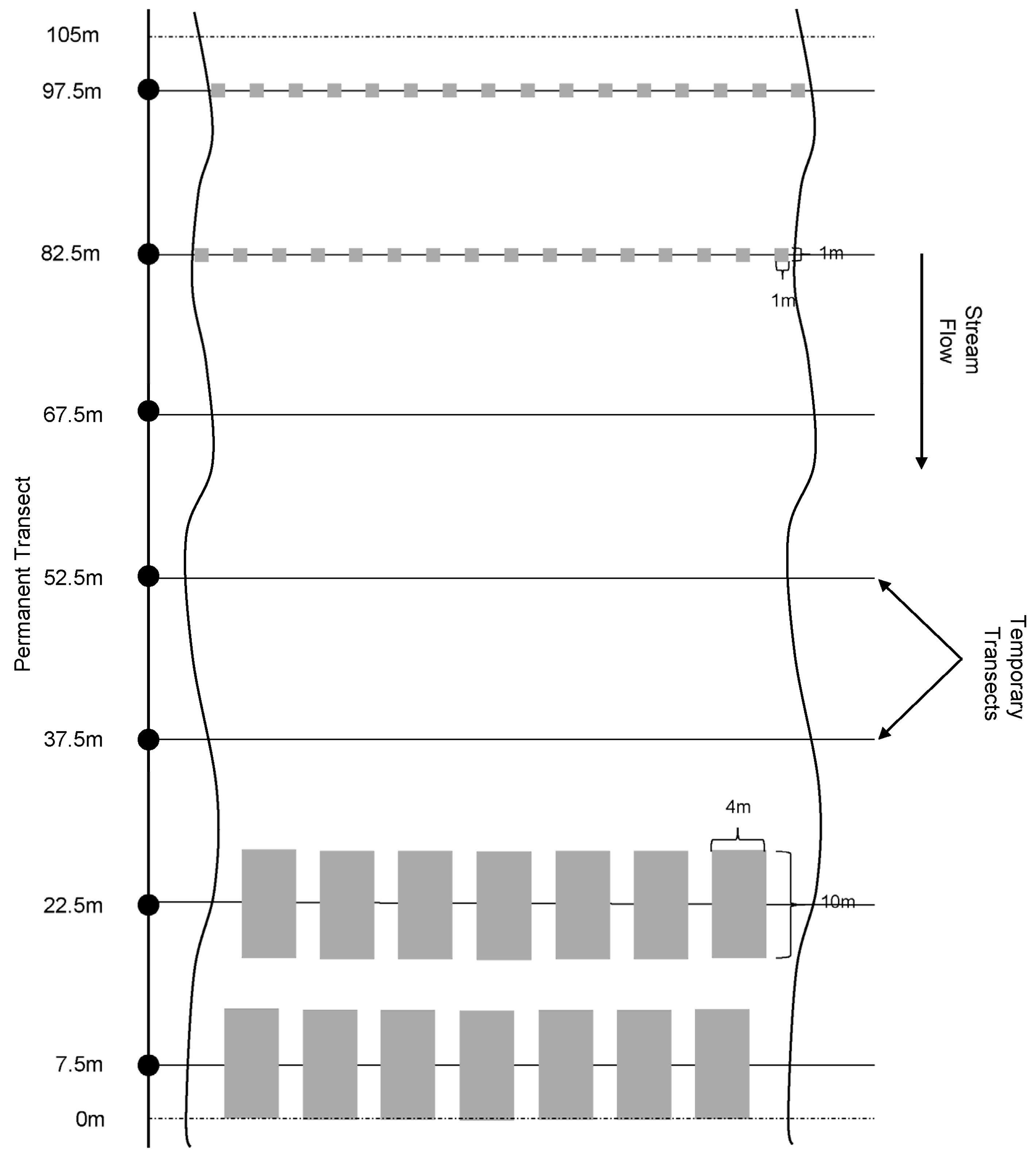
2.3.1. Description of Methods

All monitoring and analysis were conducted or supervised by us and colleagues at Virginia Tech. In our design, 12 permanent sites along a 24-km segment of the Roanoke River were selected for monitoring Roanoke logperch relative abundance and habitat conditions. Sites were chosen based on expert judgment for their suitability for Roanoke logperch. Originally, six study sites were established within each reach (C and I); however, construction plans were changed midway through the monitoring period, leaving seven control sites and five impact sites roughly uniformly distributed throughout each reach (Anderson and Angermeier 2015). Each site consisted of an erosional mesohabitat unit (i.e., riffle-run), ranging from 60 to 165 m long.
Fish sampling—With occasional exceptions due to poor sampling conditions [72], we sampled P. rex at all 12 permanent riffle-run monitoring sites in both summer (July–August) and autumn (September–October). Fish were captured by backpack electrofishing fixed-area quadrats along temporary transects at each site (Figure 3). We sampled quadrats sequentially beginning with the first quadrat on the downstream-most transect of the site, 1 m from the left river-bank (looking upstream). We sampled as many non-overlapping quadrats as would fit on a given transect, given the river width. Occasionally, areas were skipped that, based on our best judgment, exhibited velocity too high to position a seine or too low to sweep fishes into the seine. Transects were sampled sequentially in an upstream direction. During sampling of a quadrat, we positioned a 2-m-tall, 4-m-wide, 5-mm-mesh bag seine 5 m downstream from the transect. Beginning 5 m upstream from the transect, a backpack electrofisher made two or three rapid downstream passes to the seine. After electrofishing each quadrat, the seine was quickly pulled up and hauled to the river-bank, where captured fishes were processed. Captured P. rex were pooled across all quadrats in a site to determine the relative abundance of fish in the site. Relative abundance was subsequently converted to an index of population density (number ha−1) based on the area (i.e., number of quadrats) sampled at a site. We sorted captured P. rex into age classes based on TL, as follows: (1) For summer-caught logperch, fish ≤80 mm TL were Age-0 juveniles and fish >80 mm TL were Age-1+ adults or large juveniles (hereafter “adults”); (2) For autumn-caught logperch, fish ≤95 mm TL were Age-0 juveniles and fish >95 mm TL were Age-1+ adults or large juveniles (hereafter “adults”). Age-1 juveniles and Age-1+ adults cannot be reliably distinguished based on TL [60]. Very few Age-0 juveniles are captured in summer, presumably because at that life-stage fish occupy lower-velocity habitats not sampled by the electrofisher; captures increase during autumn electrofishing surveys [60].
Habitat—With occasional exceptions due to poor sampling conditions [72], we sampled microhabitat suitability for adult P. rex at all 12 permanent riffle-run monitoring sites in both summer (July–August) and autumn (September–October). Habitat measurements were made at each of a series of 1-m2 cells centered on (and occurring every 3 m along) temporary transects for each sample site (Figure 3). Within each cell, we measured the depth (cm) and water velocity (cm·s−1) at 0.6 times depth at the center of the cell and described how much of the area of the cell was covered by silt using a five-point scale similar to Rosenberger and Angermeier [58]. We also used a pebble-count method to describe substrate size at five locations equally spaced across the width of the cell. Ordinal particle sizes were assigned using a modified Wentworth scale. The five substrate measurements were then averaged to obtain a mean substrate size. We thus obtained four habitat measurements for each cell: three continuous variables (depth, velocity, and mean substrate) and one ordinal variable (silt-cover). These four variables were then used to evaluate the suitability of the cell for P. rex.
A habitat suitability index (HSI) for P. rex in the Roanoke River was developed by Ensign and Angermeier [73] based on habitat availability-versus-use data collected during underwater observation of adult P. rex. Habitat suitability mapping and analysis were accomplished using spatial interpolation procedures in ArcGIS for each sampled site. Cartesian coordinates were based on the transect georeferencing system described above, and interpolation was used to predict habitat values for unmeasured cells that occurred between measured cells. Interpolated cell size was set at 2.25 m2, providing a reasonable trade-off between map resolution and precision of the interpolation routine. We used an inverse distance-weighting interpolation routine for silt-cover, the ordinal variable, and a universal kriging interpolation routine for the three continuous variables. Once each cell in the grid was assigned its empirical or estimated habitat values, we calculated a HSI value for each cell and assigned a suitability category based on P. rex preference values. Using the cell values, we calculated the proportion of cells in a site that were in each suitability category. Statistical changes in these proportions were used to gauge change in the availability of suitable logperch habitat.

2.3.2. Construction Delays

Although RRFRP construction was originally scheduled to begin in 1990, it was continually delayed over the next 15 years. Discovery of buried toxic chemicals, a sewer installation project, and a federal budget glitch all played a role in the delay. Each year construction would be expected to start the following year, but each year another delay would surface. Although RRFRP construction (period A) ultimately did not begin until autumn 2005, USACE authorized the collection of B-period data from 1997 to 2003. This resulted in a relatively long-term baseline dataset on logperch abundance and habitat availability in the Roanoke River, which provided an opportunity to evaluate the accuracy of the initial conceptual model and assumptions and the overall adequacy of the monitoring program.

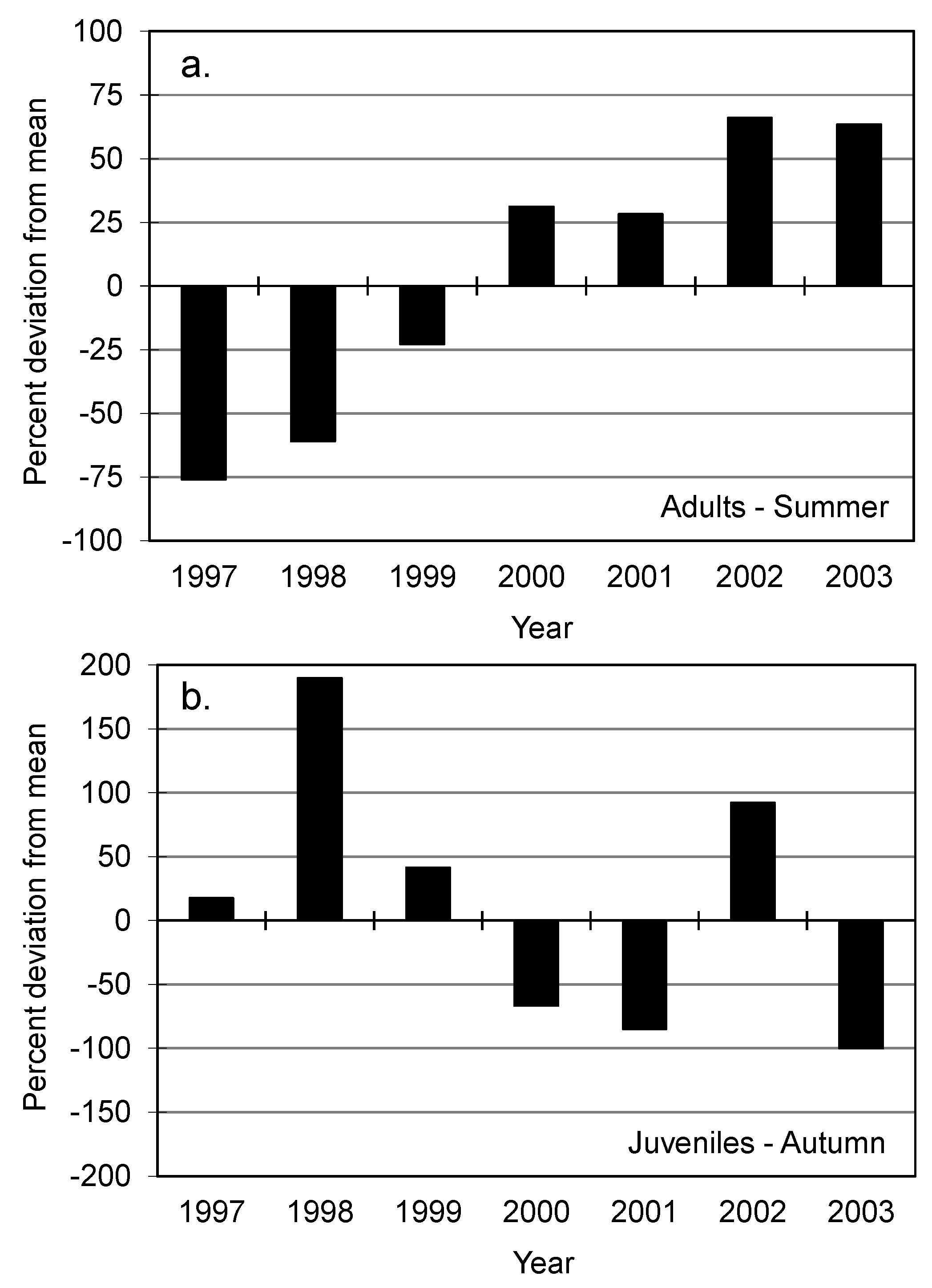
2.3.3. Results and Insights from Pre-Construction Monitoring

Our key indicator variable, estimated density of adult P. rex, was surprisingly variable across both time and space from 1997 to 2003 (Figure 4a). Certain sites consistently featured high adult P. rex densities, but interannual variance was high within all sites and did not appear to fluctuate synchronously across sites. The I reach maintained a higher mean adult density than the C reach throughout this time period, a difference that increased steadily over time. These same patterns were observed based on both summer (Figure 4a) and autumn (not shown) adult density data. High pre-construction variation made the provisions of the 1990 ITS seem questionable. Namely, the monitoring program was expected to be able to detect a 25% or greater reduction in abundance. However, when we compared each B-year’s mean adult density to the mean of all other B-years’ adult densities, we found that B-period density routinely fluctuated by more than 25% per year, and occasionally by as much as 75% per year (Figure 5). Given this background variance, we suspected that our statistical power to detect the desired effect size was low. This variation implied that (a) a single year of B monitoring would have been inadequate to characterize reference conditions; (b) perhaps many years of A monitoring would be necessary to characterize impact conditions; and (c) the 25% threshold was inappropriate for measuring compliance with the Incidental Take Permit.
Juvenile P. rex density was even more variable than adult density. We seldom captured juveniles using electrofishing methods in the summer, presumably because young fish had not yet recruited to our sampling gear, so we focused analyses on autumn capture records. The majority of the variation in juvenile density was among sites, with certain sites in both reaches (C and I) consistently producing higher densities (Figure 6). Mean density exhibited little proportional variance among years in the C reach, but fluctuated among years from nearly zero to over 40 fish ha−1 in the I reach. This between-reach difference in densities, though sizable, exhibited wide temporal variability and no temporal trend. Juvenile density was not originally intended to be an indicator variable for RRFRP impacts. Pre-construction data from the I reach suggested that this variable would have been a poor indicator at best: juvenile density in any given B year ranged from −100% to 200% of the mean of all other B years (Figure 5).
Adult habitat suitability was quantified using a five-point ordinal scale (“Poor”, “Fair”, “Suitable”, “Good”, and “Excellent”). The availability of high-quality microhabitat configurations (Good or Excellent) varied widely over B period (Figure 7). Some sites consistently featured higher percentages of high-quality habitat, but there were no consistent trends for the C or I reach to have more high-quality habitat. Rather, interannual fluctuation across sites was the predominant source of overall variation, suggesting a strong influence of hydrology. For example, a particularly low habitat-quality year in 2002 corresponded with a severe drought in the Roanoke region. Juvenile habitat availability was not assessed between 1997 and 2003.
The availability of a long (relative to the original intent) pre-construction period allowed us to test some presumed relationships from the initial conceptual model, as well as new hypotheses that emerged over this period. These analyses produced some surprising conclusions, some of which directly contradicted our initial conceptual model (Figure 1). For example, contrary to expectations, interannual variation in the availability of suitable adult habitat was negatively related to interannual variation in adult P. rex density (Figure 8; r = −0.95, p = 0.001). We did not interpret this relationship as causal, but rather as an artifact of the opposite influence of streamflow on these two variables. We expected elevated streamflow to decrease our sampling efficiency for P. rex, by causing fish to spread into habitats not typically sampled by electrofishing and by decreasing the conductivity of the water. In line with this expectation, interannual variation in mean daily streamflow (measured at USGS gauge 02055000) during the monitoring season was negatively related to interannual variation in the estimated density of adults (Figure 8; r = −0.79, p = 0.04). In contrast, we expected elevated streamflow to increase the prevalence of microhabitats estimated by HSI models to be highly suitable for adult P. rex, because depth, velocity, and low silt-cover increase with streamflow and are favorably weighted in the HSI. In line with this expectation, interannual variation in mean daily streamflow during the monitoring season was positively related to interannual variation in the mean proportion of high-quality microhabitats at sites (Figure 8; r = 0.86, p = 0.01). Beyond simply affecting sampling efficiency, streamflow appeared to affect the survival of juvenile P. rex in their first few months of life. The standard deviation of mean daily streamflow during late spring (April–June) was negatively related to the estimated mean autumn density of juvenile P. rex (Figure 8; r = −0.81, p = 0.03), presumably because unpredictable high and low flows reduced the availability or predictability of juvenile habitat or directly increased mortality of vulnerable juveniles. Potential influences of RRFRP on river hydrology were not considered in the original BO or monitoring plan, but the analyses above clearly indicated the importance of accounting for streamflow. On the other hand, there was no evidence for a relationship between adult and juvenile abundance: density of adults (stock) in summer was not significantly related to density of juveniles in autumn (recruits) (r = 0.11, p = 0.82), nor was density of juveniles in autumn of one year significantly related to density of adults in summer of the following year (r = −0.33, p = 0.53).

2.3.4. Other Opportunistic Data Collection

Besides new information stemming from pre-construction RRFRP monitoring, new scientific data relevant to the ecology and distribution of P. rex also surfaced during the RRFRP’s delay. First, there initially was scant information regarding the biology of juvenile P. rex, but subsequent studies by Rosenberger and Angermeier [58] filled in several key gaps. Notably, they established that juveniles, like adults, are relatively intolerant of heavy silt deposition, but also that the shallow, slow-flowing habitat configurations occupied by juveniles are particularly susceptible to sediment deposition. This vulnerability, and its implications for potential RRFRP impacts to P. rex, had not been considered in the original conceptual model or monitoring plan. Second, the known range of the species was expanded based on discoveries in several new streams and watersheds, and concerted sampling efforts suggested that the relative abundances of most populations were higher than originally believed [63]. Third, George and Mayden’s [74] genetic study indicated that the range fragmentation of P. rex was anthropogenic and recent in nature and that the species probably dispersed more widely in the past. These findings about the surprising mobility of P. rex have been corroborated by additional, more recent genetic and movement studies [57,65]. The 1990 BO and monitoring plan implicitly assumed that P. rex population dynamics were regulated at the site or reach scale, and did not anticipate watershed-scale metapopulation dynamics. Fourth, USFWS [75] collected stream morphology data during the RRFRP’s delay, which allowed reevaluation of the RRFRP construction plans from a geomorphological perspective that was lacking in the 1990 BO. These data indicated that impacts from RRFRP could be more pervasive than originally anticipated, including destabilizing the river channel, decreasing the river’s ability to flush fine sediment, and causing even greater silt deposition than originally predicted [75]. Although this study produced some quantitative predictions regarding changes to channel form and substrate size, it did not directly link such changes to availability of suitable P. rex habitat.

2.4. New Biological Opinion and Monitoring Plan

In 2004, considering new information that had accumulated on P. rex ecology [58], population trends and monitoring considerations in the Roanoke River [76], and river geomorphology [75], USACE reinitiated formal consultation with USFWS on the RRFRP. We were provided an opportunity to meet with USFWS and USACE to discuss previous research, outline key remaining research needs, and evaluate the efficacy of existing and new indicators for measuring RRFRP effects on P. rex abundance and habitat availability.
In 2005, USFWS issued a new BO and ITS [77]. It was again determined that the RRFRP would not jeopardize the continued existence of the species, but the 2005 BO differed from the 1990 version in several respects. First, acknowledging the considerable baseline variability in logperch abundance, and in particular that observed densities declined by as much as 75% per year during the B period, allowable take was set at 75% over one year or 25% averaged over three years. Such reductions, though seemingly dramatic, were deemed necessary to distinguish RRFRP-induced declines from natural variability. Notably, the take limit was still based simply on our catch-per-effort rather than on demographic models or population viability analyses. Second, acknowledging the potential for long-term effects of construction on logperch, perhaps accruing via impacts to juveniles or their habitat, the timeframe of monitoring was changed to three different phases: (1) one year prior; (2) every year during; and (3) 1, 2, 3, 4, 5, 7, 10, 15, and 20 years following the completion of construction. Third, given the critical lack of data on juvenile P. rex ecology, abundance, and trends in the study area, a requirement to monitor juvenile abundance and habitat availability during summer was added. Finally, acknowledging the potential impacts on river flow, geomorphology, and sediment transport, a requirement was added to monitor sediment deposition, channel morphology, and real-time turbidity at sites where P. rex abundance and habitat were monitored [78]. Though not mentioned in the revised BO, in practice we recognized the importance of accounting for hydrologic variation and began incorporating streamflow into models of population dynamics and BACI calculations.
The monitoring plan used from 2005 forward was seemingly improved (i.e., adapted) in two ways. First, by changing monitored indicators and timelines based on new knowledge, the revised plan became more scientifically defensible. Second, new indicators and methods were incorporated to facilitate the collection of novel data to fill remaining gaps in our understanding of logperch ecology (e.g., juvenile ecology, drivers of population size; Figure 1) and test a wider variety of hypotheses about mechanisms by which RRFRP might affect P. rex (Figure 2). However, the 2005 BO did not discuss how BACI-related metrics should be computed; rather, it simply asserted that “methodologies used by Roberts and Angermeier (2004) … are … valid” [77] (p. 29). One additional year’s worth of period-B data were collected in 2005, and RRFRP construction and period-A monitoring began in 2006. Although RRFRP construction concluded in 2011, we continued post-construction monitoring until 2015, when USACE discontinued funding for monitoring. Collectively, these construction and post-construction samples constituted our A sample period.
Overall, the revised monitoring plan reflected the evolution of our conceptual model of how the RRFRP might affect logperch abundance. The new model (Figure 1) incorporated (a) more factors and processes (e.g., effects of river flow on abundance of juvenile logperch); (b) shifts in the hypothesized direction of relations (e.g., abundance of adult logperch no longer limited by site-specific availability of suitable habitat); (c) more data gaps (e.g., unknown effects of RRFRP on river flow); and (d) greater uncertainty assigned to nearly all hypothesized relations. Thus, our B-period monitoring promoted significant learning but also raised many new questions and uncertainties.

2.5. Construction and Post-Construction Monitoring Period

2.5.1. Description of New Methods

Visual surveys for juveniles—Pre-construction monitoring taught us that juvenile P. rex abundance was potentially a bottleneck for population size, yet was highly dynamic in time and space and difficult to characterize using electrofishing. We therefore developed a complementary sampling approach geared toward characterizing abundance patterns earlier in the year, when P. rex had not yet transitioned to adult habitats (swift riffle-runs) and were perhaps most sensitive to hydrologic variability. This approach relied upon visual observations of juvenile P. rex during methodical shoreline walks along low-velocity pool-margin habitats [58]. We sampled juvenile P. rex at nine permanent pool sites in summer (July–August) of 2005–2015 [72]. Each of these “visual” sites was adjacent to one of the 12 sites monitored by electrofishing. Sampling was performed at base-flow conditions by two to four investigators slowly walking upstream while scanning shallow areas for juvenile P. rex. During surveys, all investigators wore polarized sunglasses, and great care was taken to not disturb the water surface. We converted juvenile P. rex observed counts to an estimate of population density by dividing the number of individuals observed by the length of river surveyed. By Age 1 or 2, P. rex shift into the riffles that are sampled by electrofishing, and become vulnerable to capture and enumeration using that method [60]. Thus, we considered visual surveys our best estimate of juvenile density in the summer (June–August) and electrofishing surveys our best estimate in autumn (September–October).
Juvenile habitat—Pre-construction monitoring and new discoveries beyond RRFRP also taught us that P. rex’s habitat needs change dramatically over ontogeny, and therefore that a fuller picture of habitat availability in the Roanoke River and potential impacts from RRFRP necessitated an additional focus on juvenile habitat. We reasoned that the shallow, slow, depositional microhabitats preferred by juveniles might be particularly vulnerable both to hydrologic disturbances and to excess RRFRP silt. We measured juvenile microhabitat conditions at six of the nine permanent pool sites [72]. We sampled each of these pools once each autumn (September–October) from 2005 to 2015. Measurements were made using a transect-based method, similar to that described above for Age-1+ habitat, except transect spacing varied among sites to achieve approximately the same number of transects (8–9) per site. At each cell, we measured depth, mean velocity, mean substrate size, and degree of silt cover. Juvenile preferences for microhabitat combinations were derived by Roberts and Angermeier [60] based on Age-0 P. rex habitat-preference data in Rosenberger and Angermeier [58]. We calculated the overall HSI score for each cell and then calculated the proportion of measured cells constituting suitable juvenile habitat. We considered any microhabitat cell with an HSI value >0 to be suitable for juvenile P. rex.

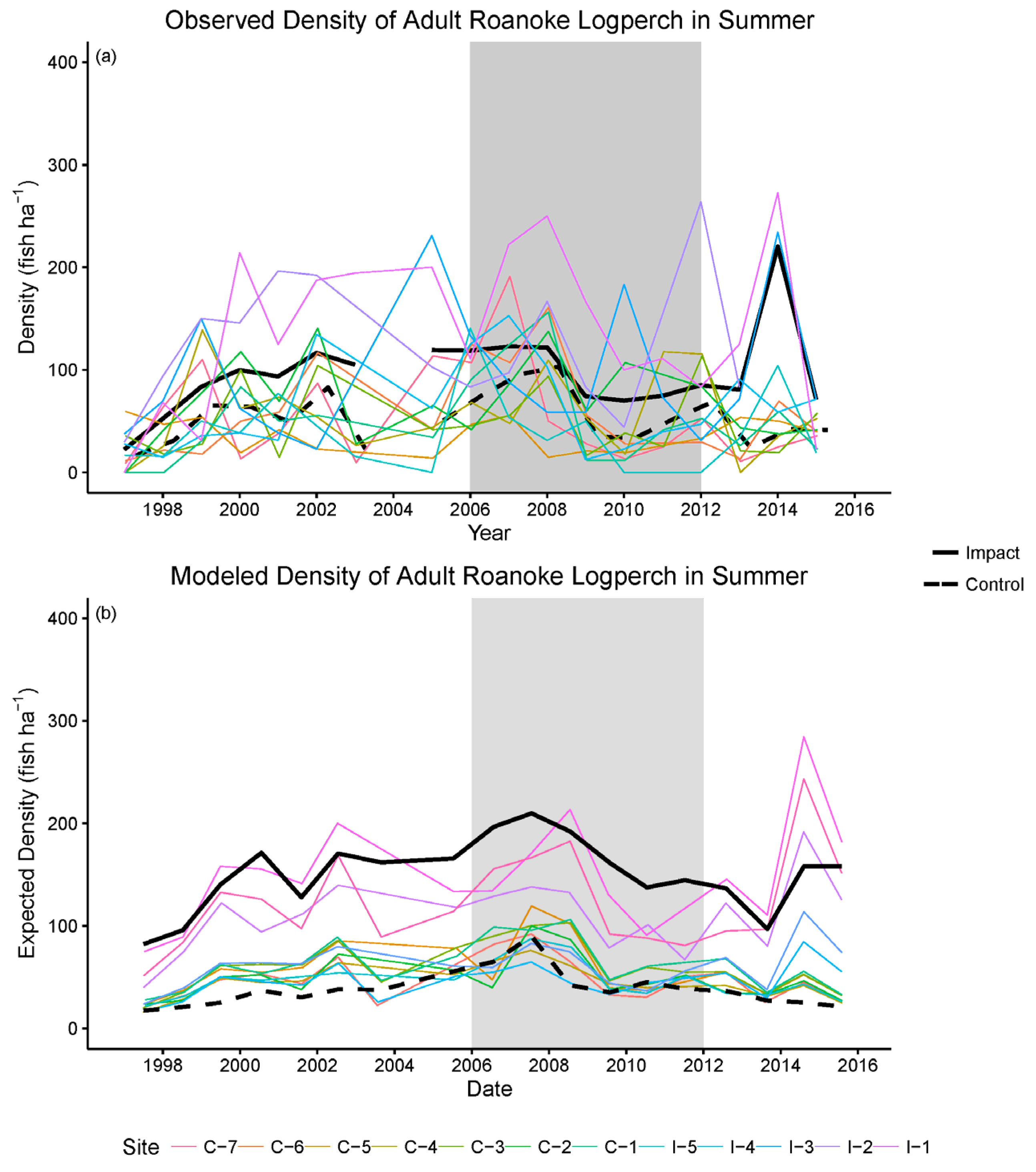
2.5.2. Results of Construction and Post-Construction Monitoring

The 19-year duration of this project provided an unprecedented look at temporal population dynamics of P. rex. Based on consideration of the full (1997–2015) dataset, spatial and temporal patterns of adult P. rex density were generally similar before and after the onset of construction (Figure 4a). As noted in the B period, during the A period, density exhibited synchronous peaks and troughs that seemed to coincide across both study reaches, suggesting that river-wide rather than local-site factors were the most important drivers of abundance.
Unlike adult density, juvenile density was monitored using two different methods during period A, electrofishing in autumn and visual surveys in summer. The two resulting datasets were not correlated across years (r = 0.04, p = 0.90) and painted different pictures of temporal variation in juvenile abundance (Figure 6). Electrofishing data nearly always indicated a low density of juveniles in the C reach, but periodic boom-bust dynamics in the I reach. Visual-survey results, on the other hand, indicated more juvenile production in C sites than electrofishing results had indicated, though this density still was typically lower than density in the I reach. Both methods indicated high interannual variation in recruitment at the river scale, and this variation was not significantly correlated with interannual variation in the density of adults for either the electrofishing (r = −0.01, p = 0.99) or visual-based (r = −0.17, p = 0.62) juvenile datasets. Observed differences between electrofishing and visual data suggested that (a) visual surveys detected juveniles more often and therefore may be more sensitive than electrofishing surveys; (b) the abundance and distribution of juveniles can change dramatically between summer (visual surveys) and autumn (electrofishing surveys); and (c) only by adopting multiple methods did a full picture of variation in juvenile abundance emerge. Despite the insights gained by visual surveys, only electrofishing data were useful for measuring potential RRFRP impacts, as visual surveys did not begin until 2005, immediately before the onset of construction. Along those lines, electrofishing data did reveal a sustained period of low juvenile production in both reaches, coinciding with the onset of RRFRP in 2006. The possibility that this represented an RRFRP impact was addressed more directly by BACI analyses (described below).
Adult habitat suitability was remarkably consistent across most period-A years, with the exception of a single-year decline in both reaches in 2008 (Figure 7), when the region was under severe drought. The prevalence of high-quality habitat continued to be negatively related to adult logperch abundance (r = −0.68, p = 0.004), due to the opposite response of these two variables to hydrologic variation. We did not begin monitoring juvenile habitat availability until 2005, as stipulated by the new BO, but like adult habitat, juvenile habitat exhibited little temporal variation through period A (Figure 7), and juvenile habitat suitability was not significantly correlated with temporal variation in the density of juveniles, whether based on electrofishing (r = −0.05, p = 0.88) or visual (r = 0.03, p = 0.93) data. Thus, the construction and post-construction data supported conclusions from the B period that microhabitat suitability does not presently limit the abundance of P. rex in the study area.

2.6. Results and Power Analyses of BACI Tests for RRFRP Impacts

At the conclusion of the monitoring program in 2015, we conducted a series of analyses to (a) test alternative hypotheses regarding potential impacts of RRFRP to Roanoke logperch; and (b) retrospectively assess our statistical power to detect impacts, given our sample sizes and levels of B-period variation. The initial conceptual model of how RRFRP activities might affect P. rex—acute mortality of adults and short-term reductions of habitat suitability that would temporarily reduce carrying capacity for adults—was overly simplistic and inconsistent with project findings. Likewise, BACI calculations, as initially conceived, were overly simplistic and ignored the possibilities that (a) construction might affect juveniles, thereby producing a lagged influence on adult density; (b) impacts might not occur all at once (i.e., pulse disturbance), but instead gradually worsen over time (i.e., press disturbance); (c) impacts might continue even after construction ends; (d) environmental factors besides RRFRP (e.g., streamflow) might influence P. rex abundance and obscure RRFRP effects and/or our ability to detect them; and (e) impacts to fish or habitat in the I reach might also have consequences for fish in the C reach. Fuller descriptions of these assumptions, and consequences of their violation for detecting change, are contained in Table 2.
As we revised our conceptual model to more fully account for factors potentially driving P. rex population dynamics, in parallel we revised our BACI analytical approach to account for new hypotheses, new variables and relationships, and complex variable interactions when testing for RRFRP impacts. Eight plausible hypotheses regarding possible impacts of the RRFRP were tested using different treatment assignments (described below) in a multivariate generalized linear mixed modeling framework. These eight hypotheses represent simplified but testable potential outcomes of the RRFRP based on the evolved conceptual model. Hypothesis 1 (mean effect) was a reformulation of the original conceptual model that sought to detect a sudden decrease in mean abundance between the B and A periods within the I reach but not the C reach (analogous to a t-test of difference in means; Figure 2a) [71]. Here, impacts were expected to occur strictly during active construction (2006–2011; A period). Hypothesis 2 (continued mean effect) was similar to Hypothesis 1, but with the A period continuing through construction (2006–2011) and post construction (2011–2015; Figure 2b). These two hypotheses represented analytical treatments typically found within BACI designs; both focused on detecting immediate impacts on adult abundance. To account for potential impacts on recruitment (i.e., survivorship of juveniles), Hypothesis 3 tested for a lagged effect. This hypothesis assumed that juveniles do not appear in samples of adults for their first two years (a reasonable assumption consistent with our observations); thus, impacts to juveniles would be observable in adult catches two years after the beginning of construction (Figure 2c). Like Hypothesis 1 and 2, this hypothesis assumed that such impacts would be drastic, only within the I reach, and could be detected beginning two years after the beginning of construction. In this hypothesis, period B includes both the construction time period and the first two years of construction (1997–2007), and period A includes from the first two years after onset of construction until two years after completion of construction (2008–2013). Hypothesis 4 (continued lagged effect) represented a lagged effect as well, but like Hypothesis 2, this effect continued into post-construction (i.e., was perpetual; 2008–2015; Figure 2d). In addition to these four hypotheses, Hypotheses 5–8 tested for similar effects but with gradual monotonic decreases in abundances (i.e., slope effects) for each of the hypotheses listed above (Figure 2e–h).
To test these eight hypotheses, eight separate models were run that also accounted for reach- and period-specific differences, additional correlates of logperch abundance, and site and year identities (treated as random effects; Table A1). In addition to these eight models, a null model that included no change in P. rex abundance was included. Models were judged based on their weight of evidence using Akaike’s Information Criterion [79] corrected for small sample size (AICc) [80]. Note that because models incorporated other factors and covariates in addition to RRFRP impact factors, support for a model did not necessarily represent support for one of the RRFRP impact hypotheses, which were included as parameters within some models (Table A1). Rather, support for impact was assessed based on the direction, magnitude, and significance of estimated regression coefficients for impact-based parameters if contained within the best-supported model(s).
Based on best-supported BACI models, all hypotheses involving RRFRP impacts demonstrated non-significant or no effects, with other factors explaining a greater proportion of the spatiotemporal variation in adult P. rex density observed. Six of the eight models representing the different hypotheses of RRFRP effects on adult density had stronger support than the null model (i.e., a model lacking any change due to measured factors; Table A2). However, only one of these models, which contained parameters representing Hypothesis 1, demonstrated any significant negative impacts of the RRFRP on adult density, and this model was not as well supported as other models in the candidate set, carrying less than 0.1% of the total model weight. According to the Hypothesis 1 model, density was higher in the A period than the B period for both C and I; however, the I density decreased during this time period and rebounded immediately during post construction.
Better-supported models (i.e., models carrying at least 5% of the total model weight) within the candidate set consistently suggested no RRFRP impacts; rather, these models demonstrated that both reaches (C and I) had declines during the hypothesized impact period (Table A2). The best-supported model within the candidate set, Hypothesis 7, contained 61.8% of the model weight. This model suggested that adult density increased during B and the first two years of construction for both reaches; however, two years after onset of construction, density monotonically decreased for both reaches and continued to decrease during post-construction. This model also implied that the rate of increase of Age-1+ logperch prior to construction in I was not as steep as in C and that recovery from the population decline was more pronounced in I than C during post-construction. The second-best supported model, Hypothesis 8, carried nearly 25% of the model weight and was also much better supported than the null model. Similar to Hypothesis 7, this model estimates that both reaches showed increasing trends in adult density prior to construction and during the first two years of construction, but decreasing trends two years after onset of construction, continuing into post-construction. However, according to this model, the slope of decrease in I was not as steep as that estimated for C during the lagged construction and post-construction phases (Table A2).
In addition to testing the eight hypotheses of RRFRP impacts, our models simultaneously tested for other covariates of adult density, and suggested that these other factors were more influential than RRFRP. For example, all models indicated a significant negative effect due to river discharge during sampling. Based on the model-averaged estimate, we would expect the number of logperch captured to decrease by 3.8% for every 10% increase in discharge (Table A2). The expected density of adult P. rex predicted by the best-supported model (Figure 4b)—which accounts for discharge and other covariates—exhibited much less spatiotemporal variation than the observed density (Figure 4a). Moreover, trends in expected density indicate that adult P. rex were consistently more abundant in I than C sites before, during, and after RRFRP construction (Figure 4b).
To evaluate our ability to detect impacts, power analyses were performed on a subset of these hypotheses. Of the eight hypotheses tested, three different ‘types’ were identified and evaluated: mean-, lagged-, and slope-based effects. Based on retrospective power analyses, statistical power to detect RRFRP impacts varied among these three impact scenarios and the magnitude of the effect-size one wished to detect. Given the variation in density during the B and A periods, the statistical power to support Hypothesis 1 (i.e., mean effect; Figure 2a) ranged from 0.05 (equivalent to the α threshold typically used for statistical significance) to detect a decline of ~0% to 0.95 to detect a decline of ~40% (Figure 9). Power to detect a lagged effect (i.e., Hypothesis 4; Figure 2d) or slope effect (i.e., Hypothesis 5; Figure 2e) was weaker and increased more slowly with increasing effect size (Figure 9). Germane to the 1990 and 2005 ITSs, statistical power to detect a 25% decline under any scenario was limited (0.4 to 0.7), whereas power to detect a 75% decline was very high (approximately 1) across all scenarios.
In summary, BACI analyses indicated that RRFRP construction did not significantly reduce the density of P. rex in the impact reach relative to the control reach, though power analyses indicated that our power to detect RRFRP-related impacts was relatively low. Independent, simultaneous research by the U.S. Geological Survey indicated a lack of RRFRP impacts to river habitat [78]. Neither suspended sediment, fine-sediment deposition, nor river-channel geomorphology changed significantly between project phases. This was attributed to a combination of effective sediment-control measures and a scarcity of channel-forming flow events during the study period [78]. Thus, RRFRP construction drew to a close without triggering further consultation or new monitoring requirements, and USACE discontinued funding for post-construction monitoring after 2015.

2.7. Applications of RRFRP Findings to P. rex Conservation

Our continual communication and coordination with USFWS and USACE throughout the RRFRP monitoring helped us provide these main stakeholders with the project-specific information they needed to complete the RRFRP while safeguarding the persistence of P. rex. We kept them apprised of recent findings, implications for potential RRFRP impacts on the species, and key uncertainties that limited our interpretation of findings and conclusions regarding impacts. Although funding for the monitoring program was always limited and generally declining over the project’s life, USFWS and USACE were willing to let us occasionally reconfigure monitoring efforts and methodology (i.e., adapt) based on our evolving knowledge of the system. Ultimately, we provided both stakeholders with the basic information they needed: science-based assurances (with appropriate caveats) that the RRFRP would not jeopardize the continued existence of P. rex.
The RRFRP monitoring program also informed P. rex conservation well beyond project-specific concerns, especially in the contexts of ecology, sampling methods, and management needs. The long duration of the RRFRP enabled us to leverage funding along the way to conduct additional studies of P. rex ecology in the upper Roanoke River subbasin. For example, we greatly expanded our knowledge of logperch movement [56,57,65,81], population viability [64], and juvenile habitat use [58]; we continue to study larval ecology and multi-scale habitat associations of P. rex [82]. We have developed and refined methodological knowledge germane to addressing conservation problems, including fish-marking techniques [57], microsatellite genetic markers [83], and estimates of P. rex detectability during electrofishing surveys. Over the years of the RRFRP we developed and compared methods for estimating P. rex abundance based on electrofishing versus snorkeling [84] and for evaluating habitat use in summer versus winter and by adults versus juveniles. Collectively, this body of work opened our eyes to the magnitude and importance of large-scale spatiotemporal dynamics of logperch populations, including the roles of environmental stochasticity and life-stage-specific dispersal. The knowledge gained via RRFRP monitoring and concurrent studies is highly valued by the USFWS, the Virginia Department of Game and Inland Fisheries, and the North Carolina Wildlife Resources Commission, the main agents of logperch conservation. Throughout the RRFRP and beyond, they have incorporated our evolving knowledge into their strategic plans for logperch conservation, including priorities for watershed restoration, additional fish surveys, and remaining research needs.

3. Key Lessons Learned

Our experience with the RRFRP taught us important lessons about how to develop and conduct a monitoring program meant to assess impacts of river channelization on an endangered fish. Below, we summarize four main lessons that we believe have broader applicability to assessments of environmental impact and restoration success in many other rivers.

3.1. Lesson 1: Plan Ahead

Pre-treatment planning, especially if coupled with preliminary monitoring, can enhance monitoring effectiveness, help avoid unforeseen pitfalls, and lead to more robust conclusions. On the front end, projects can be improved by (1) communicating with stakeholders to determine valued ecological indicators and desired and acceptable endpoints for these indicators [23]; (2) developing conceptual models based on best available science that relate indicators and endpoints to proposed alterations, and articulate the uncertainties tied to those relations; (3) collecting preliminary data sufficient to characterize spatiotemporal variation in candidate indicators, so that the statistical power and necessary sample sizes of the assessment can be estimated; (4) honestly communicating knowledge gaps, uncertainties, and options for proceeding with stakeholders; and (5) building in feedback loops that allow conceptual models, assumptions, testable hypotheses, and monitoring methods to be modified as better knowledge becomes available. We suggest that monitoring programs that explicitly include such feedback, the life-blood of adaptive management, can provide more complete answers to the questions initially driving an assessment, as well as more insights relevant to future projects, than programs that preclude or ignore feedback and learning [20,85]. Despite the utility of the five steps outlined above, incorporating them all into a pre-treatment plan is unusual. For example, Bash and Ryan [5] found that only about one-half of the projects they surveyed collected baseline data on biological, physical, or chemical measures.
Although funding may become problematic and project time lines can be short, it may be prudent to anticipate the need for (and value of) long-term pre- and post-treatment monitoring. Factors such as the generation time of focal species, level of environmental stochasticity, expected severity of changes, and precision with which indicators can be measured are typically considered in decisions about duration of monitoring periods, as all of these factors impinge upon the ability to detect change. In cases where population trends are important, the statistical power to detect temporal changes in abundance may strongly depend on the number of pre- and post-restoration surveys [86]. All these factors can be built into power analyses to provide instructive estimates of how reliable a conclusion based on a given monitoring effort might be [31,87]. Although our post-treatment monitoring lasted only a few years, our entire RRFRP experience made it clear that multi-faceted, long-term assessments are needed to address complex impacts such as those related to excess sediment and urbanization. Notably, river restoration projects commonly omit long-term assessments [7,13]. Often, the pre-treatment timeline may be most limiting, because of societal and institutional inertia, to quickly proceed with the activity. If such is the case, it is critical to assess and frankly communicate with stakeholders the statistical limitations this will place on detecting the ecological effects of the project. Finally, to facilitate proper planning, we suggest developing and adopting a priori a project-specific stepwise process analogous to that described in Table 1, then adhering to the process during the life of the project. Similar frameworks have been developed specifically for restoration projects (e.g., [23]); ours applies more generally to both restoration and impact monitoring.

3.2. Lesson 2: Develop Adaptable Conceptual and Analytical Models Early

Models provide crucial frameworks for organizing knowledge (and lack thereof), guiding study design, and analyzing data germane to any environmental problem of interest. We suggest developing both conceptual and analytical (e.g., statistical) models as early in a project’s life as possible, even if knowledge and data are sparse. We found it equally instructive to articulate what we did versus did not know, and models were valuable heuristic tools that framed subsequent data collection. Landscape-scale conceptual models can be especially helpful in illustrating linkages among remote ecosystem components, such as those that might be connected via fish migration [88]. When developing conceptual models, we suggest being humble and skeptical about what one “knows”; several of our initial presumptions at the outset of the RRFRP were eventually refuted by empirical evidence. For example, we underestimated the magnitude of environmental stochasticity, which can be accounted for by choosing appropriate sample replication, environmental indicators, and statistical models (Table 2). Models are most useful if revisited often and revised to reflect new knowledge (i.e., if adaptable). We further suggest taking advantage of any opportunities, even in other studies, to test assumptions and hypotheses embedded in conceptual models.
Conceptual models can be translated into statistical models that account for the main likely sources of variation in indicators [89]; in our case, these included river discharge, sampling efficiency, and spatial and temporal autocorrelation. Some key sources of variation may emerge as surprises, so adaptive analytical approaches that include a broad array of hypotheses and allow for inclusion of new covariates or statistical thresholds over time may be most instructive. We found it very helpful to develop an exhaustive set of explicit, alternative, a priori hypotheses based on ecological phenomena (not merely statistical thresholds such as p < 0.05), so that we could anticipate alternative potential findings and use them to support one or more of these hypotheses. Our hypotheses were derived directly from our conceptual models. This process of hypothesis development facilitated learning and reduced the need for a posteriori “arm-waving” to explain findings. We suggest that applying a similar approach elsewhere may help alleviate the common problem of reaching contradictory conclusions at the end of efforts to assess project success [13].

3.3. Lesson 3: Recognize Limits of Study Scope

Ecological phenomena are products of factors and processes interacting across multiple scales. For wild populations, key scaling dimensions include space, time, and ontogeny. Because it is infeasible for a given monitoring program to cover all relevant extents of these dimensions, program designers must narrow the scope (i.e., specific spatial extent, duration, and life stages) to reflect the most important questions of interest. Here, importance is determined by stakeholders and potential outcomes of the proposed alteration [20]. Portions of key dimensions excluded from monitoring can still be considered in conceptual and analytical models, and may be crucial in interpreting results.
Accounting for catchment-wide processes and linkages was perhaps our greatest scaling problem in the context of interpreting our findings, and we suspect this situation is common among projects that are not catchment-wide in scope. For example, potential positive effects of local habitat enhancement are often swamped by larger-scale geomorphic or physicochemical factors [12,90]. Population and geophysical processes commonly operate across entire catchments, whereas local sites offer limited views and understanding of those processes [2,91]. At the outset of the RRFRP, we were especially ignorant of large-scale processes driving logperch dynamics, such as stage-specific dispersal, ontogenetic shifts in habitat use, and range-wide flux in abundance, any of which could influence (or even dominate) the dynamics we observed in the study area. In retrospect, we learned to (a) more carefully think about how early (least understood) life-stages of P. rex might be affected by the RRFRP; (b) consider the possibility that juvenile and/or adult P. rex commonly disperse over long distances, perhaps transcending the boundaries of our C and I study reaches; and (c) consider the implications of these knowledge gaps for interpreting our findings. Dispersal of P. rex, in particular, raised a thorny analytical problem: if sites are linked by dispersal, they cannot be treated as independent (as in a typical BACI analysis) unless dispersal is accounted for explicitly. Thus, for future projects, conceptual and analytical models need to account for dispersal of focal species in the spatial configuration of monitoring sites.
Because limiting factors for populations vary with the spatiotemporal extent considered and are often unknown, we suggest that extra care may be needed to ensure that scopes of assessments of impact or restoration are commensurate with scopes of the biological responses of interest. That is, designers of monitoring programs might be mindful of scale mis-matches among processes regulating factors of interest, selected ecological indicators, and methods used to measure indicators [13,40]. In our case, availability of “suitable habitat” may limit P. rex distribution range-wide, but as measured, did not seem to be limiting within Roanoke River sites over the temporal duration of the study. In other occupied watersheds, where silt-free habitat configurations are rarer [63], habitat suitability may be a more important limiting factor. Our measures of habitat availability focused on microhabitat within sites, but we lacked measures of habitat availability at reach- and catchment-wide extents. Thus, the positive relationship we expected to observe between habitat availability and logperch abundance may not have emerged simply because of a mis-match between the scales (extent and grain) of measurement (micro-scale variation in habitat) versus ecological process (macro-scale regulation of P. rex population dynamics) [34].

3.4. Lesson 4: Carefully Choose Analytical Frameworks and Tools

Analytical frameworks and tools facilitate, but can also limit, objective, statistically valid interpretation of findings. Choosing the best analytical approach requires familiarity with its assumptions and potential pitfalls relative to the data to be analyzed (Table 2) [17], and this choice may change as new data and approaches become available. Further, using multiple analytical frameworks can provide insights that use of only a single framework can mask [89]. In some cases, choice of an appropriate analytic framework may need to be made before the design of a study. For example, ecologists have become increasing aware of the issue of incomplete detection or capture oif focal animals [92,93,94,95,96]. Approaches to correct for such biases generally require either a repeated-measures or capture-recapture design (but see [97,98]). Decisions of whether more samples should be collected at sites within a season (where a site is assumed closed to population or occupancy changes) versus sampling more sites each season are difficult, but the benefits of a repeated-measures or capture-recapture design (e.g., less arm waving) can outweigh the costs (e.g., additional sampling).
Although widely applied to environmental assessments, application of the BACI framework within a riverine system required us to make several simplistic and untenable assumptions (e.g., impacts were applied suddenly and uniformly to the I reach, C and I reaches were demographically independent, and environmental factors other than the RRFRP were constant; Table 2) that are probably unmet in many other BACI applications or in other analyses aimed at assessing effects of unreplicated alterations [99]. These assumptions can lead to biased conclusions that may be vetted by adopting alternative analytical frameworks or testing for impacts on multiple ecological indicators (e.g., adults and juveniles). Within riverine systems, control or reference sites are often upstream of impact reaches [100]. Such designs may be appropriate when the river or stream is homogenous over the study area (e.g., habitat is similar between reaches) and the indicator of interest does not move between reaches. In cases where this is not true, a BACI framework may not be appropriate, and a more simplified design (i.e., before versus after) [101] may be needed, albeit with the potential cost of lower statistical power and less reliable inference. In any event, conducting power analyses early in the monitoring process will typically lead to quicker learning, clearer interpretation of findings, and more robust conclusions about the ecological change of interest [31,32,102,103].

4. Conclusions: Robust Monitoring in the Real World?

Our findings indicate that long monitoring periods and flexible conceptual models and sampling designs may be critical components of a monitoring program seeking to measure demographic responses of threatened biota in dynamic river environments. Long timelines and flexibility were fortuitous post hoc additions to our study. In the absence of this extensive dataset and experimental freedom, we would not have been able to conduct valid statistical tests or gained as much knowledge regarding the biology of P. rex. Compared to many programs that monitor environmental impact of restoration success, our case study may have been unusually conducive to learning. Our agency collaborators (USFWS and USACE) were willing to incorporate an adaptive management philosophy into the experimental design, monitoring metrics, and detection-of-impact calculations of the RRFRP. A long monitoring time frame, which at first was opportunistic, was subsequently embraced by USFWS. For example, the required post-construction monitoring phase went from nonexistent in the 1990 BO [70] to 20 years long in the 2005 BO [77].
We posit that adoption of a planning framework, and set of guiding principles similar to that described in Table 1 and Table 2 (see also [6,8,13]) will lead to more cost-effective, scientifically-defensible monitoring. However, we fully recognize that widespread integration of these principles into monitoring studies will be challenging. Existing institutional cultures, legal frameworks, and funding constraints may not readily accommodate an adaptive management philosophy. If pre-existing data are particularly poor (as in this study), an adaptive approach could require adaptively defining restoration success or construction impact after monitoring or the project has started. Implementation of the ESA and similar laws usually involves little flexibility, and stakeholders directly affected by these laws may be uneasy about such uncertainty [26]. Levels of acceptable take are typically defined explicitly, at a project’s outset, in the ITS or permit. This document is considered a contract with assurances, not subject to renegotiation based on additional data. Nonetheless, ecological assessments are fraught with uncertainty [104], and the implications of this uncertainty for decision-making are a burden that should be shared among all parties. One solution could be to issue ITSs that explicitly require incremental assessments of take levels and take thresholds during a project’s lifetime, essentially granting a series of provisional incidental take allowances instead of a single blanket allowance. Such statements would likely benefit from a more structured approach to decision-making [22,28] than what is typically utilized in take assessments [33].
Conservation managers will also likely face resistance to the notion of long pre- and post-project monitoring phases, despite the importance of such data for characterizing baseline variability and lagged effects, respectively [105]. There typically is strong institutional inertia to complete a project while money, votes, and public support are in place. The time necessary to collect adequate pre-project monitoring data may delay project onset, which may be undesirable to some stakeholders. On the other hand, delaying a project to accommodate more monitoring could reduce the risk of project failure (i.e., failure to adequately measure the ecological element of interest) or the risk of unanticipated future financial costs (e.g., to correct for an initially inadequate study design), and in this light may be more palatable to stakeholders. Regardless, money spent on monitoring may be perceived as taking away from other, more focal aspects of a project, such that monitoring, especially post-project, can be underfunded in restoration budgets. In detection-of-impact studies, post-project effects may be critical, but after project completion, conservation managers have limited leverage to mandate sustained monitoring. For example, although the 2005 BO for the RRFRP required post-construction monitoring in years 1, 2, 3, 4, 5, 7, 10, 15, and 20 after construction ceased [77], USACE discontinued funding for monitoring after year 4. Our communications with USACE staff at that time indicated their decision was based primarily on the limited evidence of project impacts. Even if monitoring activities are adequately funded from the start, this budget allocation is likely to be fixed, which precludes any expansion of monitoring scope mid-project. In our case, because monitoring funding was generally fixed (and declining) throughout the project, we expanded the study scope to new variables “discovered” to potentially be important (e.g., juvenile habitat use and availability) by shifting field time and resources away from monitoring other variables deemed less important (e.g., adult habitat availability in autumn). Such sacrifices may not be possible or advisable in other monitoring studies, which reemphasizes the importance of pre-treatment planning, preliminary data, and sound conceptual models, to increase the likelihood that the most important dependent and independent variables are measured properly.
Given these challenges, is robust and informative monitoring possible in the real world? We suggest that scientists can play three main roles in facilitating scientifically defensible monitoring. First, scientists can help define the “optimal” monitoring design to accomplish stakeholder objectives. To this end, scientific input at the planning phase is crucial (Table 1). There, scientists can work with stakeholders to define project goals, relevant response variables (e.g., population size, water quality), and criteria for defining success. Then, to the extent possible given best available scientific knowledge and preliminary data from the system of interest, scientists can (1) develop conceptual models relating key processes and elements of the system; (2) design an optimal monitoring experimental design for detecting the desired or acceptable degree of change in the response variable(s) of interest, with the desired statistical precision; and (3) convey this information to stakeholders in as quantitative and probabilistic way as data allow. Ultimately, stakeholders will decide whether this optimal design is pursued, or whether certain study features get compromised due to logistical or budgetary considerations (e.g., shorter monitoring period, inflexible monitoring plan).
Second, scientists have a responsibility to convey to stakeholders the consequences of monitoring compromises, framed in terms of reduced statistical power to detect desired or acceptable changes in valued ecological elements. If valued elements cannot be tracked with meaningful statistical power, stakeholders may still proceed with the project, but would do so with the understanding that they would be wasting resources to monitor those elements. In this case, stakeholders could either decide on an alternative element that can be measured with greater precision and accuracy, or accept that the project may have unmeasured ecological benefits or impacts, but that such changes cannot form the basis for evaluating the project. In essence, scientists can help make these hard choices explicit to stakeholders.
Third, scientists can work to change the institutional culture surrounding monitoring requirements and policies. To be scientifically valid and informative to stakeholders, monitoring requirements need to focus on clearly demonstrating effects or trends of interest (e.g., positive effects for restoration or lack of effects due to potential impacts); these outcomes are crucial to future decisions about project funding and approval. In the case of imperiled species, scientists might also work with agency biologists (e.g., USFWS) to focus monitoring requirements around variables that can be interpreted in terms of species persistence (e.g., population size, area of critical habitat) rather than simpler relative-abundance indices. If key variables or reference points are unknown, biologists can work to explicitly treat monitoring programs as adaptive learning opportunities [105]. Finally, our findings and the work of others indicate that key biological and ecological processes play out over potentially large spatiotemporal extents [91], to which monitoring studies should be well matched [7,19]. This matching process would necessitate a shift from monitoring over anthropocentric timeframes (fiscal years) to monitoring over ecocentric (hydrologic cycles) and biocentric timeframes (organism generations).

Acknowledgments

We thank the USACE for funding much of this work, the USACE and USFWS for their willingness to adapt models and monitoring protocols as new information came to light, and dozens of technicians for assistance with fieldwork over the years, which was carried out under the auspices of Institutional Animal Care and Use Committee protocol 11-035-FIW at Virginia Tech. Brett Albanese, Bill Ensign, Greg Galbreath, Amanda Rosenberger, and Barbara Blood were particularly influential in the development, implementation, and evolution of this study. The Virginia Cooperative Fish and Wildlife Research Unit is jointly sponsored by the U.S. Geological Survey, Virginia Polytechnic Institute and State University, Virginia Department of Game and Inland Fisheries, and Wildlife Management Institute. Use of trade names or commercial products does not imply endorsement by the U.S. government.

Author Contributions

P.A., J.R. and G.A. conceived and designed the experiments; J.R. and G.A. performed the experiments and analyzed the data; P.A., J.R. and G.A. wrote the paper.

Conflicts of Interest

The authors declare no conflict of interest. The funding sponsors participated in the experimental design of the study, but did not participate in the collection, analyses, or interpretation of data, the writing of the manuscript, or the decision to publish the results.

Abbreviations

The following abbreviations are used in this manuscript:
AMAdaptive Management
ANOVAAnalysis of Variance
BACIBefore-After-Control-Impact
BOBiological Opinion
ESAEndangered Species Act
GLMMGeneralized Linear Mixed Model
ITSIncidental Take Statement
RRFRPRoanoke River Flood Reduction Project
USACEUnited States Army Corps of Engineers
USFWSUnited States Fish and Wildlife Service
USGSUnited States Geological Survey
VAVirginia

Appendix

This section describes in detail the variables and modeling procedures used to test alternative BACI hypotheses about the effect of the Roanoke River Flood Reduction Project (RRFRP), as well as other ecological and sampling features, on empirical captures of Roanoke logperch (Percina rex) in the Roanoke River.
Table A1. Variable names, data types, associated hypotheses (Hyp.) from the Methods and Figure 2, modeled levels, and descriptions of variables used for testing hypotheses regarding impacts of the RRFRP on abundance of adult and juvenile Roanoke logperch. Variables that represent potential impacts of the RRFRP on Roanoke logperch are underlined in the “Modeled Levels” column. I, Con., and Cont. Con stand for impact reach, active construction project phase, and continued construction project phase, respectively.
VariableTypeHyp.Modeled LevelsDescription
DischargeContinuous1–8-Discharge at the time of sample.
SeasonFactor1–8FallSamples taken in September–October. Summer samples are the reference category (i.e., intercept)
ReachFactor1–8ISamples taken in the impact reach (I). Control reach (C) samples are the reference category.
Project PhaseFactor1Con.Samples taken during the active construction project phase (2006–2011). Pre-construction (Pre Con.) samples (1997–2005) are the reference category.
Post Con.Samples taken during the post-construction project phase (2012–2015). Pre-construction samples (1997–2005) are the reference category.
Continued Project PhaseFactor2Cont. Con.Samples taken during the construction or post-construction project phase. Pre-construction samples are the reference category.
Lagged Project PhaseFactor3Lag Con.Samples taken at least two years after the onset of construction to two years after the completion of construction (i.e., 2008–2013). Pre-construction samples and the first two years of construction samples are the reference category.
Lag Post Con.Samples taken at least two years after the completion of construction (2014–2015). Pre-construction samples and the first two years of construction samples are the reference category.
Continued Lagged Project PhaseFactor4Cont. Lag Con.Samples taken at least two years after the onset of construction through post-construction (i.e., 2008–2015). Pre-construction samples and the first two years of construction samples are the reference category.
YearContinuous--Continuous variable representing the year of study.
Project Phase SlopeInteraction5Pre Con. × YearInteraction between the Pre. Con level of Project Phase and Year.
Con. × YearInteraction between the Con level of Project Phase and Year.
Post Con. × YearInteraction between the Post Con level of Project Phase and Year.
Continued Project Phase SlopeInteraction6Pre Con. × YearInteraction between the Pre. Con level of Continued Project Phase and Year.
Cont. Con. × YearInteraction between the Cont. Con. level of Continued Project Phase and Year.
Lagged Project Phase SlopeInteraction7Lag Pre Con. × YearInteraction between the Lag Pre Con. level of Lagged Project Phase and Year.
Lag Con. × YearInteraction between the Lag Con. level of Lagged Project Phase and Year.
Lag Post Con. × YearInteraction between the Lag Post Con. level of Lagged Project Phase and Year.
Continued Lagged Project Phase SlopeInteraction8Lag Pre Con. × YearInteraction between the Lag Pre Con. level of Continued Lagged Phase and Year.
Cont. Lag Con. × YearInteraction between the Cont. Lag Con. level of Continued Lagged Project Phase and Year.
Mean EffectInteraction1I × Con.Interaction between the I level of reach and the Con. level of Project Phase.
Continued Mean EffectInteraction2I × Cont. Con.Interaction between the I level of reach and the Cont. Con. level of Continued Project Phase.
Lagged Mean EffectInteraction3I × Lag Con.Interaction between the I level of reach and the Lag Con. level of Lagged Project Phase.
Continued Lagged Mean EffectInteraction4I × Lag Cont. Con.Interaction between the I reach and the Cont. Lag Con. level of Continued Lagged Project Phase.
Slope EffectInteraction5I × Pre Con. × YearInteraction between the I level of reach, the Pre Con. level of Project Phase, and the year.
I × Con. × YearInteraction between the I level of reach, the Con. level of Project Phase, and the year.
I × Post Con. × YearInteraction between the I level of reach, the Post Con. level of Project Phase, and the year.
Continued Slope EffectInteraction6I × Pre Con. × YearInteraction between the I level of reach, the Pre Con. level of Continued Project Phase, and the year.
I × Cont. Con. × YearInteraction between the I level of reach, the Cont. Con. level of Continued Project Phase, and the year.
Lagged Slope EffectInteraction7I × Lag Pre Con. × YearInteraction between the I level of reach, the Lag Pre Con. level of Lagged Project Phase, and the year.
I × Lag Con. × YearInteraction between the I level of reach, the Lag Con. level of Lagged Project Phase, and the year.
I × Lag Post Con. × YearInteraction between the I level of reach, the Lag Post Con. level of Lagged Project Phase, and the year.
Continued Lagged Slope EffectInteraction8I × Pre Con. × YearInteraction between the I level of reach, the Lag Pre Con. level of Continued Lagged Project Phase, and the year.
I × Cont. Con. × YearInteraction between the I level of reach, the Cont. Lag Con. level of Continued Lagged Project Phase, and the year.
Table A2. Model structure to analyze observed counts of adult P. rex with respective parameter estimates, log likelihood, relative difference in Akaike’s Information Criterion values corrected for small sample size (AICc), and model weight for each of the nine models representing different RRFRP impact hypotheses and the null model (i.e., a model containing no impact terms). Pre. Con., Con. and Post Con. refer to the project phases: pre-construction, construction, and post construction, respectively; see Table A1 for variable name descriptions. Different combinations of the phases were used for before and after treatments within the BACI design. Parameters that represent impacts of the RRFRP are underlined and significant parameters are in bold (α = 0.05). Model performance statistics can be interpreted as follows: log-likelihood (ℓ) represents the overall fit of the model (higher is better) but is not penalized for the complexity of the model; relative difference (Δi) in AICc represents the relative difference (lower is better) of the criterion from the best-supported model (i.e., the model with the lowest AICc), where AICc is a penalized criterion of model performance that is based on the log-likelihood, the number of parameters, and the sample size; and model weight (wi) is roughly equivalent to the posterior probability of the model being the best-supported model in the candidate set. Dashes indicate variables not present in models.
VariableModels
Null12345678
Intercept−1.59−1.70−1.70−1.50−1.50−0.98−1.02−1.09−1.08
Discharge−0.16−0.15−0.16−0.16−0.16−0.20−0.20−0.20−0.20
Season (Fall)−0.07−0.06−0.06−0.06−0.07−0.10−0.11−0.09−0.10
Reach (I)0.520.560.560.430.430.290.180.270.21
Con. Phase-0.39-------
Cont. Con. Phase--0.20------
Lag Con. Phase---−0.11-----
Cont. Lag Con. Phase----−0.21----
Post Con. Phase-−0.17-------
Lag Post Con. Phase---−0.62-----
Pre Con. × Year-----0.680.64--
Lag Pre Con. × Year-------0.590.60
Con. × Year-----−0.78---
Cont. Con. × Year------−0.63--
Lag Con. × Year-------−0.56-
Cont. Lag Con. × Year--------−0.59
Post Con. × Year-----−0.63---
Lag Post Con. × Year-------−0.63-
I × Con.-−0.31-------
I × Cont. Con.--−0.07------
I × Lag Con.---0.02-----
I × Cont. Lag Con.----0.21----
I × Post Con.-0.37-------
I × Lag Post Con.---0.87-----
I × Pre Con. × Year-----−0.22−0.31--
I × Lag Pre Con. × Year-------−0.25−0.29
I × Con. × Year-----0.09---
I × Cont. Con. × Year------0.49--
I × Lag Con. × Year-------0.26-
I × Cont. Lag Con. × Year--------0.48
I × Post Con. × Year-----0.47---
I × Lag Post Con. × Year-------0.63-
Model Performance
−925.6−915.0−924.6−916.3−923.8−907.6−910.8−905.8−908.7
Δi27.6414.4429.5216.9830.003.655.880.0001.82
wi<0.001<0.001<0.001<0.001<0.0010.0970.0330.6180.249

References

  1. Malmqvist, B.; Rundle, S. Threats to the running water ecosystems of the world. Environ. Conserv. 2002, 29, 134–153. [Google Scholar] [CrossRef]
  2. Allan, J.D. Landscapes and riverscapes: The influence of land use on stream ecosystems. Annu. Rev. Ecol. Evol. Syst. 2004, 35, 257–284. [Google Scholar] [CrossRef]
  3. Dudgeon, D.; Arthington, A.H.; Gessner, M.O.; Zawabata, Z.-I.; Knowler, D.J.; Lévêque, C.; Naiman, R.J.; Prieur-Richard, A.-H.; Soto, D.; Stiassny, M.L.J.; et al. Freshwater biodiversity: Importance, threats, status and conservation challenges. Biol. Rev. 2006, 81, 163–182. [Google Scholar] [CrossRef] [PubMed]
  4. Closs, G.P.; Angermeier, P.L.; Darwall, W.R.T.; Balcombe, S.R. Why are freshwater fish so threatened? In Conservation of Freshwater Fishes; Closs, G.P., Krkosek, M., Olden, J., Eds.; Cambridge University Press: London, UK, 2015; pp. 37–75. [Google Scholar]
  5. Bash, J.S.; Ryan, C.M. Stream Restoration and Enhancement Projects: Is Anyone Monitoring? Environ. Manag. 2002, 29, 877–885. [Google Scholar] [CrossRef] [PubMed]
  6. Downs, P.W.; Kondolf, G.M. Post-project appraisals in adaptive management of river channel restoration. Environ. Manag. 2002, 29, 477–496. [Google Scholar] [CrossRef]
  7. Bernhardt, E.S.; Palmer, M.A.; Allan, J.D.; The National River Restoration Science Synthesis Working Group. Restoration of U.S. Rivers: A national synthesis. Science 2005, 308, 636–637. [Google Scholar] [CrossRef] [PubMed]
  8. Palmer, M.A.; Bernhardt, E.; Allan, J.D.; The National River Restoration Science Synthesis Working Group. Standards for ecologically successful river restoration. J. Appl. Ecol. 2005, 42, 208–217. [Google Scholar] [CrossRef]
  9. Alexander, A.; Alexander, G.; Allan, J.D. Ecological success in stream restoration: Case studies from the Midwestern United States. Environ. Manag. 2007, 40, 245–255. [Google Scholar] [CrossRef] [PubMed]
  10. Bernhardt, E.; Sudduth, E.; Palmer, M.; Allan, J.; Meyer, J.; Alexander, G.; Follastad Shah, J.; Hassett, B.; Jenkinson, R.; Lave, R.; et al. Restoring rivers one reach at a time: Results from a survey of US river restoration practitioners. Restor. Ecol. 2007, 15, 482–493. [Google Scholar] [CrossRef]
  11. Palmer, M.A.; Menninger, H.L.; Bernhardt, E. River restoration, habitat heterogeneity and biodiversity: A failure of theory or practice? Freshw. Biol. 2010, 55, 205–222. [Google Scholar] [CrossRef]
  12. Feld, C.K.; Birk, S.; Bradley, D.C.; Hering, D.; Kail, J.; Marzin, A.; Melcher, A.; Nemitz, D.; Pedersen, M.L.; Pletterbauer, F.; et al. From natural to degraded rivers and back again: A test of restoration ecology theory and practice. Adv. Ecol. Res. 2011, 44, 119–209. [Google Scholar]
  13. Morandi, B.; Piégay, H.; Lamouroux, N.; Vaudor, L. How is success or failure in river restoration projects evaluated? Feedback from French restoration projects. J. Environ. Manag. 2014, 137, 178–188. [Google Scholar] [CrossRef] [PubMed]
  14. Hering, D.; Aroviita, J.; Baattrup-Pedersen, A.; Brabec, K.; Buijse, T.; Ecke, F.; Friberg, N.; Gielczewski, M.; Januschke, K.; Köhler, J.; et al. Contrasting the roles of section length and instream habitat enhancement for river restoration success: A field study of 20 European restoration projects. J. Appl. Ecol. 2015, 52, 1518–1527. [Google Scholar] [CrossRef]
  15. Karr, J.R.; Fausch, K.D.; Angermeier, P.L.; Yant, P.R.; Schlosser, I.J. Assessing Biological Integrity in Running Waters: A Method and Its Rationale; Illinois Natural History Survey: Champaign, IL, USA, 1986. [Google Scholar]
  16. Lake, P.S.; Bond, N.; Reich, P. Linking ecological theory with stream restoration. Freshw. Biol. 2007, 52, 597–615. [Google Scholar] [CrossRef]
  17. Underwood, A.J. Beyond BACI: The detection of environmental impacts on populations in the real, but variable, world. J. Exp. Mar. Biol. Ecol. 1992, 161, 145–178. [Google Scholar] [CrossRef]
  18. Rosenfeld, J.S.; Hatfield, T. Information needs for assessing critical habitat of freshwater fish. Can. J. Fish. Aquat. Sci. 2006, 63, 683–698. [Google Scholar] [CrossRef]
  19. Jansson, R.; Nilsson, C.; Malmqvist, B. Restoring freshwater ecosystems in riverine landscapes: The roles of connectivity and recovery processes. Freshw. Biol. 2007, 52, 589–596. [Google Scholar] [CrossRef]
  20. Walters, C.J. Adaptive Management of Renewable Resources; MacMillan: New York, NY, USA, 1986. [Google Scholar]
  21. Haney, A.; Power, R.L. Adaptive management for sound ecosystem management. Environ. Manag. 1996, 20, 879–886. [Google Scholar] [CrossRef]
  22. Conroy, M.J.; Peterson, J.T. Decision Making in Natural Resource Management: A Structured, Adaptive Approach; John Wiley and Sons: Hoboken, NJ, USA, 2013. [Google Scholar]
  23. Woolsey, S.; Capelli, F.; Gonser, T.; Hoehn, E.; Hostmann, M.; Junker, B.; Paetzold, A.; Roulier, C.; Schweizer, S.; Tiegs, S.D.; et al. A strategy to assess river restoration success. Freshw. Biol. 2007, 52, 752–769. [Google Scholar] [CrossRef]
  24. Jansson, R.; Backx, H.; Boulton, A.J.; Dixon, M.; Dudgeon, D.; Hughes, F.M.R.; Nakamura, K.; Stanley, E.H.; Tockner, K. Stating mechanisms and refining criteria for ecologically successful river restoration: A comment on Palmer et al. (2005). J. Appl. Ecol. 2005, 42, 218–222. [Google Scholar] [CrossRef]
  25. Wohl, E.; Angermeier, P.L.; Bledsoe, B.; Kondolf, G.M.; MacDonnell, L.; Merritt, D.M.; Palmer, M.A.; Poff, N.L.; Tarboton, D. River restoration. Water Resour. Res. 2005, 41, 1–12. [Google Scholar] [CrossRef]
  26. Smallwood, K.S.; Beyea, J.; Morrison, M.L. Using the best scientific data for endangered species conservation. Environ. Manag. 1999, 24, 421–435. [Google Scholar] [CrossRef]
  27. Wilhere, G.F. Adaptive management in habitat conservation plans. Conserv. Biol. 2002, 16, 20–29. [Google Scholar] [CrossRef]
  28. Runge, M.C. An introduction to adaptive management for threatened and endangered species. J. Fish Wildl. Manag. 2011, 2, 220–233. [Google Scholar] [CrossRef]
  29. Tear, T.H.; Karieva, P.; Angermeier, P.L.; Comer, P.; Czech, B.; Kautz, R.; Landon, L.; Mehlman, D.; Murphy, K.; Ruckelshaus, M.; et al. How much is enough? The recurrent problem of setting measurable objectives in conservation. BioScience 2005, 55, 835–849. [Google Scholar] [CrossRef]
  30. Lobon-Cervia, J. Why, when and how do fish populations decline, collapse and recover? The example of brown trout (Salmo trutta) in Rio Chaballos (northwestern Spain). Freshw. Biol. 2009, 54, 1149–1162. [Google Scholar] [CrossRef]
  31. Ham, K.D.; Pearsons, T.N. Can reduced salmonid population abundance be detected in time to limit management impacts? Can. J. Fish. Aquat. Sci. 2000, 57, 17–24. [Google Scholar] [CrossRef]
  32. Reed, J.M.; Blaustein, A.R. Biologically significant population declines and statistical power. Conserv. Biol. 1997, 11, 281–282. [Google Scholar] [CrossRef]
  33. Harding, E.K.; Crone, E.E.; Elderd, B.D.; Hoekstra, J.M.; McKerrow, A.J.; Perrine, J.D.; Regetz, J.; Rissler, L.J.; Stanley, A.G.; Walters, E.L.; et al. The scientific foundations of habitat conservation plans: A quantitative assessment. Conserv. Biol. 2001, 15, 488–500. [Google Scholar] [CrossRef]
  34. Orth, D.J. Ecological considerations in the development and application of instream flow-habitat models. Regul. Rivers Res. Manag. 1987, 1, 171–181. [Google Scholar] [CrossRef]
  35. Rosenfeld, J. Assessing the habitat requirements of stream fishes: An overview and evaluation of different approaches. Trans. Am. Fish. Soc. 2003, 132, 953–968. [Google Scholar] [CrossRef]
  36. Newcomb, T.J.; Orth, D.J.; Stauffer, D.F. Habitat Evaluation. In Analysis and Interpretation of Freshwater Fisheries Data; Guy, C.S., Brown, M.L., Eds.; American Fisheries Society: Bethesda, MD, USA, 2007; pp. 843–886. [Google Scholar]
  37. Pretty, J.L.; Harrison, S.S.C.; Shepherd, D.J.; Smith, C.; Hildrew, A.G.; Hey, R.D. River rehabilitation and fish populations: Assessing the benefit of instream structures. J. Appl. Ecol. 2003, 40, 251–265. [Google Scholar] [CrossRef]
  38. Miller, S.W.; Budy, P.; Schmidt, J.C. Quantifying macroinvertebrate responses to instream habitat restoration: Applications of meta-analysis to river restoration. Restor. Ecol. 2010, 18, 8–19. [Google Scholar] [CrossRef]
  39. Lepori, F.; Palm, D.; Brännäs, E.; Malmquist, B. Does restoration of structural heterogeneity in streams enhance fish and macroinvertebrate diversity? Ecol. Appl. 2005, 15, 2060–2071. [Google Scholar] [CrossRef]
  40. Rios-Touma, B.; Prescott, C.; Axtell, S.; Kondolf, G.M. Habitat restoration in the context of watershed prioritization: The ecological performance of urban stream restoration projects in Portland, Oregon. River Res. Appl. 2015, 31, 755–766. [Google Scholar] [CrossRef]
  41. US Environmental Protection Agency (USEPA). Wadeable Streams Assessment: A Collaborative Survey of the Nation’s Streams; EPA 841-B-06-002; Office of Research and Development and Office of Water, US Environmental Protection Agency: Columbia, WA, USA, 2006.
  42. Jelks, H.L.; Walsh, S.J.; Burkhead, N.M.; Contreras-Balderas, S.; Díaz-Pardo, E.; Hendrickson, D.A.; Lyons, J.; Mandrak, N.E.; McCormick, F.; Nelson, J.S.; et al. Conservation status of imperiled North American freshwater and diadromous fishes. Fisheries 2008, 33, 372–407. [Google Scholar] [CrossRef]
  43. Waters, T.F. Sediment in Streams: Sources, Biological Effects, and Control; American Fisheries Society: Bethesda, MD, USA, 1995. [Google Scholar]
  44. Henley, W.; Patterson, M.; Neves, R.; Lemly, A.D. Effects of sedimentation and turbidity on lotic food webs: A concise review for natural resource managers. Rev. Fish. Sci. 2000, 8, 125–139. [Google Scholar] [CrossRef]
  45. Rabeni, C.F.; Smale, M.A. Effects of siltation on stream fishes and the potential mitigating role of the buffering riparian zone. Hydrobiologia 1995, 303, 211–219. [Google Scholar] [CrossRef]
  46. Lapointe, M.; Bergeron, N.; Berube, F.; Pouliot, M.; Johnston, P. Interactive effects of substrate sand and silt contents, redd-scale hydraulic gradients, and interstitial velocities on egg-to-emergence survival of Atlantic salmon (Salmo salar). Can. J. Fish. Aquat. Sci. 2004, 61, 2271–2277. [Google Scholar] [CrossRef]
  47. Kemp, P.; Sear, D.; Collins, A.; Naden, P.; Jones, I. The impacts of fine sediment on riverine fish. Hydrol. Process. 2011, 25, 1800–1821. [Google Scholar] [CrossRef]
  48. Arnold, J.G.; Moriasi, D.N.; Gassman, P.W.; Abbaspour, K.C.; White, M.J.; Srinivasan, R.; Santhi, C.; Harmel, R.D.; van Griensven, A.; van Liew, M.W.; et al. SWAT: Model use, calibration, and validation. Trans. Am. Soc. Agric. Biol. Eng. 2012, 55, 1491–1508. [Google Scholar]
  49. Hamilton, S.K. Biogeochemical time lags may delay responses of streams to ecological restoration. Freshw. Biol. 2012, 57 (Suppl. S1), 43–57. [Google Scholar] [CrossRef]
  50. Brown, L.R.; Cuffney, T.F.; Coles, J.F.; Fitzpatrick, F.; McMahon, G.; Steuer, J.; Bell, A.H.; May, J.T. Urban streams across the USA: Lessons learned from studies in 9 metropolitan areas. J. N. Am. Benthol. Soc. 2009, 28, 1051–1069. [Google Scholar] [CrossRef]
  51. Violin, C.R.; Cada, P.; Sudduth, E.B.; Hassett, B.A.; Penrose, D.L.; Bernhardt, E.S. Effects of urbanization and urban stream restoration on the physical and biological structure of stream ecosystems. Ecol. Appl. 2011, 21, 1932–1949. [Google Scholar] [CrossRef] [PubMed]
  52. Wang, L.; Lyons, J.; Kanehl, P.; Bannerman, R. Impacts of urbanization on stream habitat and fish across multiple spatial scales. Environ. Manag. 2001, 28, 255–266. [Google Scholar] [CrossRef]
  53. Morgan, R.P.; Cushman, S.E. Urbanization effects on stream fish assemblages in Maryland, USA. J. N. Am. Benthol. Soc. 2005, 24, 643–655. [Google Scholar] [CrossRef]
  54. Walsh, C.J.; Fletcher, T.D.; Ladson, A.R. Stream restoration in urban catchments through redesigning stormwater systems: Looking to the catchment to save the stream. J. N. Am. Benthol. Soc. 2005, 24, 690–705. [Google Scholar] [CrossRef]
  55. Wheeler, A.P.; Angermeier, P.L.; Rosenberger, A.E. Impacts of new highways and subsequent landscape urbanization on stream habitat and biota. Rev. Fish. Sci. 2005, 13, 141–164. [Google Scholar] [CrossRef]
  56. Roberts, J.H.; Angermeier, P.L.; Hallerman, E.M. Distance, dams and drift: What structures populations of an endangered, benthic stream fish? Freshw. Biol. 2013, 58, 2050–2064. [Google Scholar] [CrossRef]
  57. Roberts, J.H.; Rosenberger, A.E.; Albanese, B.W.; Angermeier, P.L. Movement patterns of endangered Roanoke logperch (Percina rex). Ecol. Freshw. Fish 2008, 17, 374–381. [Google Scholar] [CrossRef]
  58. Rosenberger, A.E.; Angermeier, P.L. Ontogenetic shifts in habitat use by the endangered Roanoke logperch Percina rex. Freshw. Biol. 2003, 48, 1563–1577. [Google Scholar] [CrossRef]
  59. Burkhead, N.M. Ecological Studies of Two Potentially Threatened Fishes (the Orangefin madtom Noturus gilberti and Roanoke logperch Percina rex) Endemic to the Roanoke River Drainage; Final Report; U.S. Army Corps of Engineers: Wilmington, NC, USA, 1983. [Google Scholar]
  60. Roberts, J.H.; Angermeier, P.L. Assessing Impacts of the Roanoke River Flood Reduction Project on the Endangered Roanoke Logperch; Final Report to the Wilmington District; U.S. Army Corps of Engineers: Wilmington, NC, USA, 2006. [Google Scholar]
  61. Roberts, J.H.; Rosenberger, A.E. Threatened fishes of the world: Percina rex (Jordan and Evermann 1989) (Percidae). Environ. Biol. Fishes 2008, 83, 439–440. [Google Scholar] [CrossRef]
  62. Jenkins, R.E.; Burkhead, N.M. Freshwater Fishes of Virginia; American Fisheries Society: Bethesda, MD, USA, 1994. [Google Scholar]
  63. Rosenberger, A.E. An Update to the Roanoke Logperch Recovery Plan; Final Report; U.S. Fish and Wildlife Service: Gloucester, VA, USA, 2007.
  64. Roberts, J.H.; Angermeier, P.L.; Anderson, G.B. Population viability analysis for endangered Roanoke logperch. J. Fish Wildl. Manag. 2016. [Google Scholar] [CrossRef]
  65. Roberts, J.H.; Angermeier, P.L.; Hallerman, E.M. Extensive dispersal of Roanoke logperch (Percina rex) inferred from genetic marker data. Ecol. Freshw. Fish 2016, 25, 1–16. [Google Scholar] [CrossRef]
  66. Schlosser, I.J.; Angermeier, P.L. Spatial variation in demographic processes of lotic fishes: Conceptual models, empirical evidence, and implications for conservation. Am. Fish. Soc. Symp. 1995, 17, 392–401. [Google Scholar]
  67. Corrigan, P. The Floods of November 1985: Then and Now; National Oceanic and Atmospheric Administration, National Weather Service: Silver Spring, MD, USA, 2010. Available online: http://www.erh.noaa.gov/rnk/hydro/Flood%20of%201985_Then-Now.pdf (accessed on 31 January 2016).
  68. United States Army Corps of Engineers (USACE). Roanoke River Upper Basin, Virginia, Headwaters Area, Flood Damage Reduction—General Design Memorandum Volumes I and II; U.S. Army Corps of Engineers: Wilmington, NC, USA, 1989. [Google Scholar]
  69. Jenkins, R.E. Roanoke Logperch Percina rex (Jordan and Evermann 1889); Final Report; U.S. Fish and Wildlife Service: Gloucester, VA, USA, 1977.
  70. United States Fish and Wildlife Service (USFWS). Biological Opinion on the Roanoke River Upper Basin, Headwaters Area, Flood Damage Reduction Project, in Roanoke, Virginia; U.S. Army Corps of Engineers: Wilmington, NC, USA, 1990. [Google Scholar]
  71. Stewart-Oaten, A.; Murdoch, W.W.; Parker, K.R. Environmental impact assessment: Pseudoreplication in time? Ecology 1986, 67, 929–940. [Google Scholar] [CrossRef]
  72. Anderson, G.B.; Angermeier, P.L. Assessing Impacts of the Roanoke River Flood Reduction Project on the Endangered Roanoke Logperch; Final Report; U.S. Army Corps of Engineers: Wilmington, NC, USA, 2015. [Google Scholar]
  73. Ensign, W.E.; Angermeier, P.L. Summary of Population Estimation and Habitat Mapping Procedures for the Roanoke River Flood Reduction Project; Final Report to the Wilmington District; U.S. Army Corps of Engineers: Wilmington, NC, USA, 1994. [Google Scholar]
  74. George, A.L.; Mayden, R.L. Conservation Genetics of Four Imperiled Fishes of the Southeast; Final Report; U.S. Forest Service: Washington, DC, USA, 2003. [Google Scholar]
  75. United States Fish and Wildlife Service (USFWS). Analysis of U.S. Army Corps of Engineers’ Roanoke River Flood Reduction Project with Respect to Natural Channel Morphology; U.S. Army Corps of Engineers: Wilmington, NC, USA, 2003. [Google Scholar]
  76. Roberts, J.H.; Angermeier, P.L. Monitoring Effects of the Roanoke River Flood Reduction Project on the Endangered Roanoke Logperch Percina rex; Final Report; U.S. Army Corps of Engineers: Wilmington, NC, USA, 2004. [Google Scholar]
  77. United States Fish and Wildlife Service (USFWS). Biological Opinion on the Roanoke River Upper Basin, Headwaters Area, Flood Damage Reduction Project, in Roanoke, Virginia; U.S. Army Corps of Engineers: Wilmington, NC, USA, 2005. [Google Scholar]
  78. Jastram, J.D.; Krstolic, J.L.; Moyer, D.L.; Hyer, K.E. Fluvial Geomorphology and Suspended-Sediment Transport during Construction of the Roanoke River Flood Reduction Project in Roanoke, Virginia, 2005–2012; Scientific Investigations Report 2015–5111; United States Geological Survey: Reston, VA, USA, 2015.
  79. Akaike, H. A new look at the statistical model identification. IEEE Trans. Autom. Control 1974, 19, 716–723. [Google Scholar] [CrossRef]
  80. Hurvich, C.M.; Tsai, C.-L. Regression and time series model selection in small samples. Biometrika 1989, 76, 297–307. [Google Scholar] [CrossRef]
  81. Ensign, W.E.; Leftwich, K.N.; Angermeier, P.L.; Dolloff, C.A. Factors influencing stream fish recovery following a large-scale disturbance. Trans. Am. Fish. Soc. 1997, 126, 895–907. [Google Scholar] [CrossRef]
  82. Argentina, J.E.; Roberts, J.H. Habitat Associations for Young-of-Year Roanoke Logperch in Roanoke River; Final Report; Virginia Department of Game and Inland Fisheries: Richmond, VA, USA, 2014. [Google Scholar]
  83. Dutton, D.J.; Roberts, J.H.; Angermeier, P.L.; Hallerman, E.M. Microsatellite markers for the endangered Roanoke logperch Percina rex (Percidae) and their potential utility for other darter species. Mol. Ecol. Resour. 2008, 8, 831–834. [Google Scholar] [CrossRef] [PubMed]
  84. Ensign, W.E.; Angermeier, P.L.; Dolloff, C.A. Use of line transect methods to estimate abundance of benthic stream fishes. Can. J. Fish. Aquat. Sci. 1995, 52, 213–222. [Google Scholar] [CrossRef]
  85. Walters, C.J.; Holling, C.S. Large-scale management experiments and learning by doing. Ecology 1990, 71, 2060–2068. [Google Scholar] [CrossRef]
  86. Vaudor, L.; Lamouroux, N.; Olivier, J.; Forcellini, M. How sampling influences the statistical power to detect changes in abundance: An application to river restoration. Freshw. Biol. 2015, 60, 1192–1207. [Google Scholar] [CrossRef]
  87. Korman, J.; Higgins, P.S. Utility of escapement time series data for monitoring the response of salmon populations to habitat alteration. Can. J. Fish. Aquat. Sci. 1997, 54, 2058–2067. [Google Scholar] [CrossRef]
  88. Kimmerer, W.J.; Murphy, D.D.; Angermeier, P.L. A Landscape-level model for ecosystem restoration in the San Francisco Estuary and its watershed. San Franc. Estuary Watershed Sci. 2005, 2. Available online: http://repositories.cdlib.org/jmie/sfews/vol3/iss1/art2 (accessed on 29 April 2016). [Google Scholar]
  89. Skalski, J.R. Statistical considerations in the design and analysis of environmental damage assessment studies. J. Environ. Manag. 1995, 43, 67–85. [Google Scholar] [CrossRef]
  90. Lorenz, A.W.; Feld, C.K. Upstream river morphology and riparian land use overrule local restoration effects on ecological status assessment. Hydrobiologia 2013, 704, 489–501. [Google Scholar] [CrossRef]
  91. Fausch, K.D.; Torgersen, C.E.; Baxter, C.V.; Li, H.W. Landscapes to riverscapes: Bridging the gap between research and conservation of stream fishes. BioScience 2002, 52, 483–498. [Google Scholar] [CrossRef]
  92. Cormack, R. Estimates of survival from the sighting of marked animals. Biometrika 1964, 51, 429–438. [Google Scholar] [CrossRef]
  93. Jolly, G.M. Explicit estimates from capture-recapture data with both death and immigration-stochastic model. Biometrika 1965, 52, 225–247. [Google Scholar] [CrossRef] [PubMed]
  94. Seber, G.A.F. A note on the multiple-recapture census. Biometrika 1965, 52, 249–259. [Google Scholar] [CrossRef] [PubMed]
  95. MacKenzie, D.I.; Nichols, J.D.; Royle, J.A.; Pollock, K.H.; Bailey, L.L.; Hines, J.E. Occupancy Estimation and Modeling: Inferring Patterns and Dynamics of Species Occurrence; Academic Press/Elsvier: Burlington, MA, USA, 2006. [Google Scholar]
  96. Kéry, M.; Schmidt, B.R. Imperfect detection and its consequences for monitoring for conservation. Community Ecol. 2008, 9, 207–216. [Google Scholar] [CrossRef] [Green Version]
  97. Lele, S.R.; Moreno, M.; Bayne, E. Dealing with detection error in site occupancy surveys: What can we do with a single survey? J. Plant Ecol. 2012, 5, 22–31. [Google Scholar] [CrossRef]
  98. Sólymos, P.; Lele, S.; Bayne, E. Conditional likelihood approach for analyzing single visit abundance survey data in the presence of zero inflation and detection error. Environmetrics 2012, 23, 197–205. [Google Scholar] [CrossRef]
  99. Stewart-Oaten, A.; Bence, J.R.; Osenberg, C.W. Assessing effects of unreplicated perturbations: No simple solutions. Ecology 1992, 73, 1396–1404. [Google Scholar] [CrossRef]
  100. Baldigo, B.P.; Warren, D.R.; Ernst, A.G.; Mulvihill, C.I. Response of fish populations to natural channel design restoration in streams of the Catskill Mountains, New York. N. Am. J. Fish. Manag. 2008, 28, 954–969. [Google Scholar] [CrossRef]
  101. Smith, E.P. BACI designs. In Encyclopedia of Environmetrics; El-shaarawi, A.H., Piegorsch, W.W., Eds.; Wiley: Chickester, UK, 2002; pp. 141–148. [Google Scholar]
  102. Baldigo, B.P.; Warren, D.R. Detecting the response of fish assemblages to stream restoration: Effects of different sampling designs. N. Am. J. Fish. Manag. 2008, 28, 919–934. [Google Scholar] [CrossRef]
  103. Peterman, R.M. Statistical power analysis can improve fisheries research and management. Can. J. Fish. Aquat. Sci. 1990, 47, 2–15. [Google Scholar] [CrossRef]
  104. Ludwig, D.; Hilborn, R.; Walters, C. Uncertainty, resource exploitation, and conservation: Lessons from history. Ecol. Appl. 1993, 3, 547–549. [Google Scholar] [CrossRef] [PubMed]
  105. Evans, D.M.; Che-Castaldo, J.P.; Crouse, D.; Davis, F.W.; Epanchin-Niell, R.; Flather, C.H.; Frohlich, R.K.; Goble, D.D.; Li, Y.W.; Male, T.D.; et al. Species recovery in the United States: Increasing the effectiveness of the Endangered Species Act. Issues Ecol. 2016, 20, 1–28. [Google Scholar]
Figure 1. The (a) original (1990), and (b) revised (2005) conceptual models describing how ecological factors, including the Roanoke River Flood Reduction Project (RRFRP), affect the population dynamics of adult and juvenile Roanoke logperch (Percina rex). Arrows indicate influences and symbols in black indicate hypothesized directions of influence: positive (+), negative (−), or unknown (?). Symbols in red indicate results of empirical tests of relationships: positive (+), negative (−), no significant relationship (NS), or not tested (?).
Water 08 00240 g001
Figure 2. Eight plausible impacts of RRFRP construction on Roanoke logperch (Percina rex) abundance: (a) a mean effect, a decrease in mean adult abundance during active construction (grey rectangle) in the impact reach (I) but not in the control reach (C); (b) a continued mean effect, a decrease in mean adult abundance in construction and post-construction in I but not in C; (c) a lagged mean effect, a decrease in mean adult abundance during active construction in I but with a two-year lag after the onset of construction; (d) a continued lagged mean effect, a decrease in mean adult abundance during active construction and post-construction in I but with a two-year lag after the onset of construction; (e) a slope effect, a monotonic decrease in adult abundance during active construction in I but not in C; (f) a continued slope effect, a monotonic decrease in adult abundance during active construction and post-construction in I but not in C; (g) a lagged slope effect, a monotonic decrease in adult abundance during active construction in I but with a two-year lag after the onset of construction; and (h) a continued lagged slope effect, a monotonic decrease in adult abundance in I during active construction and post-construction but with a two-year lag after the onset of construction. Pre-construction (Pre-Con.), active construction (Con.), and post-construction (Post-Con.) refer to 1997–2005, 2006–2011, and 2012–2015, respectively. Solid and dashed lines indicate hypothesized periods of RRFRP non-impact and impact, respectively.
Water 08 00240 g002
Figure 3. Layout of a hypothetical 105-m-long sample site, indicating: site boundaries (dashed horizontal lines), permanent stakes (solid circles), permanent transects (bold lines), temporary transects (solid horizontal lines), example quadrats for fish sampling (bottom, shaded rectangles), and example cells for habitat sampling (top, shaded squares). Wavy vertical lines represent wetted edges of the river channel.
Water 08 00240 g003
Figure 4. (a) Observed and (b) modeled temporal variation in the mean density of adult Roanoke logperch (Percina rex) at impact (I) and control (C) sites during summer of 1997–2003 and 2005–2015. Individual site observations are shown in color and are referenced by their respective reaches with consecutive numbers ordered upstream to downstream. Solid and dashed black lines represent I and C reach means, respectively. The active RRFRP construction period is shown as a gray rectangle. Modeled densities were calculated as the expected abundance from the best-supported model (Model 7; see Table A2) divided by the area sampled and converted to the units of fish catch per hectare (ha). Thus, these trends have incorporated the influences of model variation due to streamflow, season, and RRFRP phase.
Water 08 00240 g004
Figure 5. Proportional variation in (a) summer adult and (b) autumn juvenile Roanoke logperch (Percina rex) density during the pre-construction period (1997–2003) of the RRFRP. Each year’s mean density [across impact (I) sites] is expressed as a percentage of the mean of all other years’ densities at I sites. Density frequently fluctuated by >25% per year prior to construction, suggesting that we would be unable to detect a 25% reduction due to construction impacts.
Water 08 00240 g005
Figure 6. Observed temporal variation in the mean density of juvenile Roanoke logperch (Percina rex) based on (a) visual surveys in summer and (b) electrofishing surveys in autumn at impact (I) and control (C) sites during 1997–2003 and 2005–2015. Individual site observations are shown in color and are referenced by their respective reaches with consecutive numbers ordered upstream to downstream. Solid and dashed black lines represent I and C reach means, respectively. The active RRFRP construction period is shown as a gray rectangle. For clarity, the density axes are on a square-root scale.
Water 08 00240 g006
Figure 7. Mean percentage of available microhabitats classified as (a) high quality (i.e., excellent or good) for adult Roanoke logperch (Percina rex) and (b) suitable for juvenile P. rex at impact (I; filled circles) and control (C; open circles) sites from 1997 to 2003 and 2005 to 2014. Individual site estimates are shown in color and are referenced by their respective reaches with consecutive numbers ordered upstream to downstream. Error bars represent 95% confidence intervals, assuming a normal distribution. The period of active RRFRP construction is shown as a gray rectangle.
Water 08 00240 g007
Figure 8. Bivariate relationships between ecological predictor variables and (ac) density of adult Roanoke logperch (Percina rex) in summer (fish ha−1); (d) percent availability of high-quality adult P. rex habitat in summer (%); and (ef) density of juvenile P. rex in autumn (fish ha−1). Each plot uses data collected from 1997 to 2003 to test relationships hypothesized in the original (1990) conceptual model (see Figure 1) to be important for regulating P. rex population dynamics. Each data point represents the mean across all 12 permanent sampling sites for one year. Solid lines indicate regression slopes significantly different from zero; dotted lines indicate non-significant relationships. Variables are further explained in the text.
Water 08 00240 g008
Figure 9. Results from a retrospective statistical power analysis to detect three hypothesized effects of the RRFRP using a generalized linear mixed modeling approach: (a) a mean effect (Hypothesis 1 and Figure 2a); (b) a lagged effect (Hypothesis 3 and Figure 2c); and (c) a slope effect (Hypothesis 5 and Figure 2e).
Water 08 00240 g009
Table 1. Steps and considerations in designing and implementing an adaptive long-term monitoring program to assess environmental impacts or restoration actions in rivers. Table entries reflect our experiences in the Roanoke River Flood Reduction Project (RRFRP). Learning can occur throughout the process but mostly occurs during implementation.
Phases and StepsKey ConsiderationsPotential PitfallsRRFRP Examples
Planning Phase
Step 1. Communicate with stakeholders to identify valued biological and environmental attributes and desired or acceptable endpoints.Identify (a) attributes expected to respond to proposed alteration, (b) realistic endpoints, and (c) endpoints based on non-arbitrary, ecologically meaningful criteria.Selection of attributes that (a) cannot be indexed with measurable indicators or (b) are unresponsive to proposed alteration, or (c) are arbitrary or unrealistic, so results have unclear interpretations. 25%–75% annual reduction in adult logperch abundance had no clear implication for population viability.
Step 2. Define spatiotemporal scope and objectives of proposed alteration.Social, economic, and environmental factors may limit potential alterations.Unanticipated factors may impinge on the project’s scope.Construction was delayed for several years.
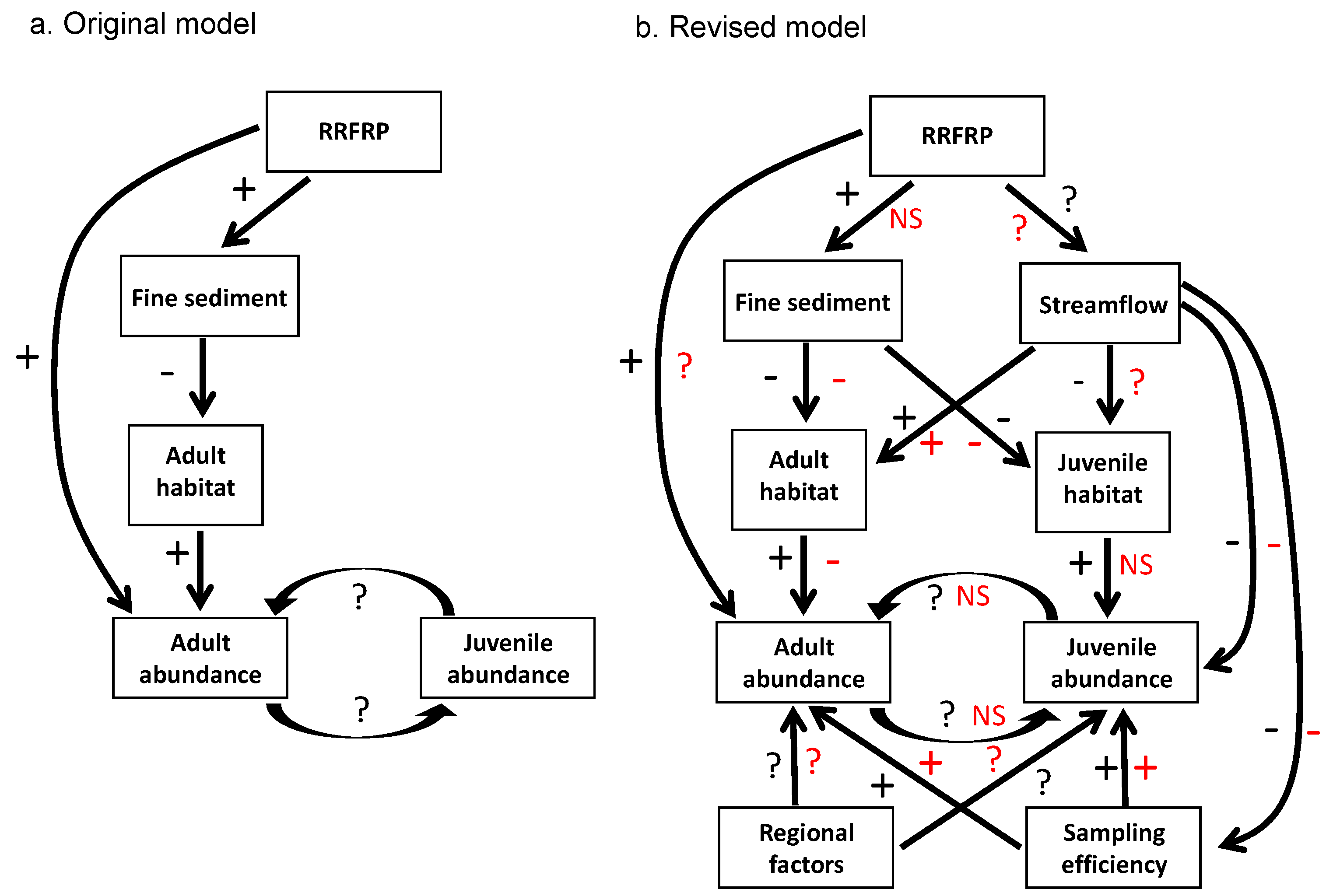
Step 3. Develop initial conceptual model relating major factors and processes to each other, based on best available knowledge (see Figure 1a).Account for all important direct and indirect linkages among factors, processes, and proposed alteration.Knowledge gaps may result in conceptual model failing to account for (a) non-linear or indirect relations between known factors or (b) unknown factors.Lack of basic dispersal information on logperch.
Lagged effects of construction on logperch abundance.
Logperch recruitment and detection driven by river flow.
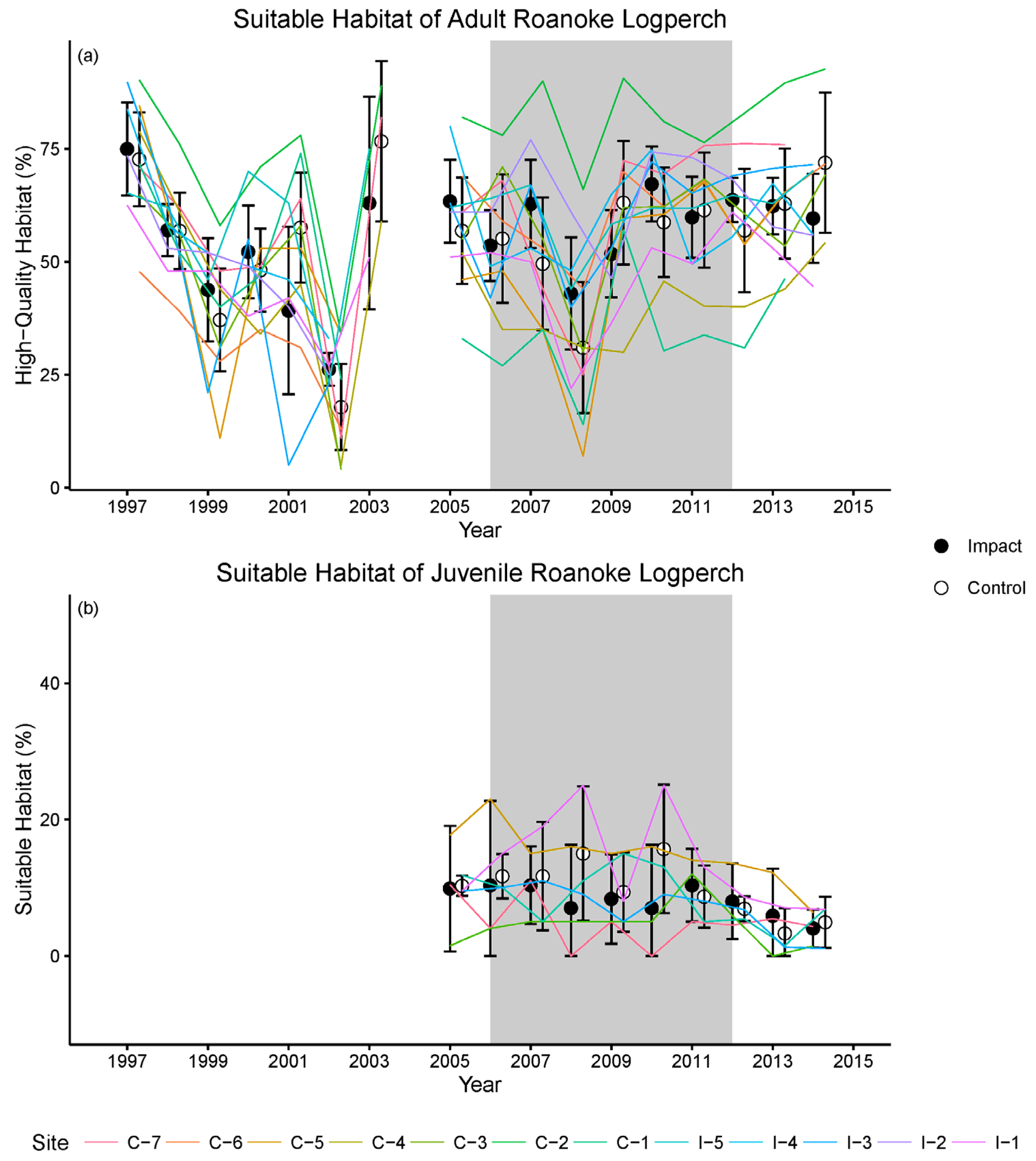
Step 4. Choose specific biological and environmental indicators to represent factors and processes of interest, including any thresholds for acceptability or success.Identify measurable indicators that (a) can be measured with sufficient precision and accuracy and (b) index the status of valued attributes.Selection of indicators that (a) cannot be measured with sufficient accuracy or precision or (b) do not covary with valued attributes.Logperch abundance was difficult to measure.
Relation between habitat availability and logperch abundance obscured by river flow.
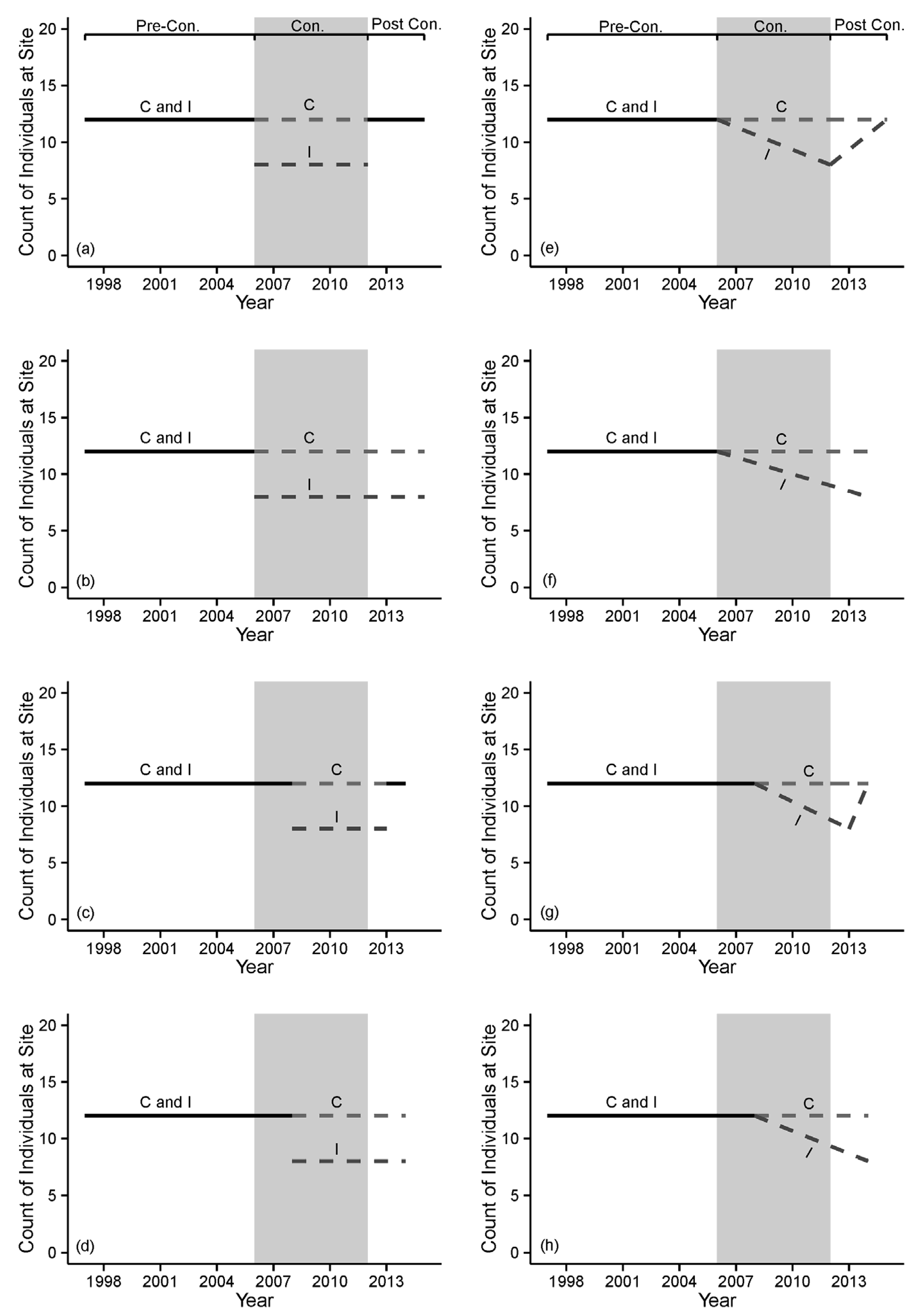
Step 5. Develop comprehensive set of testable alternative hypotheses regarding effects of proposed alteration on indicators.Develop hypotheses that account for all reasonable types and routes of influence of the proposed alteration.
Ensure that all potential results can be interpreted via alternative hypotheses (avoid surprises).
Overly simplistic hypotheses may fail to account for important types and routes of influences.
Failure to consider a priori all potential results may necessitate post hoc arm-waving and weaken inferences.
Original BACI test assumed sudden, constant effects on indicators; revised tests included lagged and gradual effects.
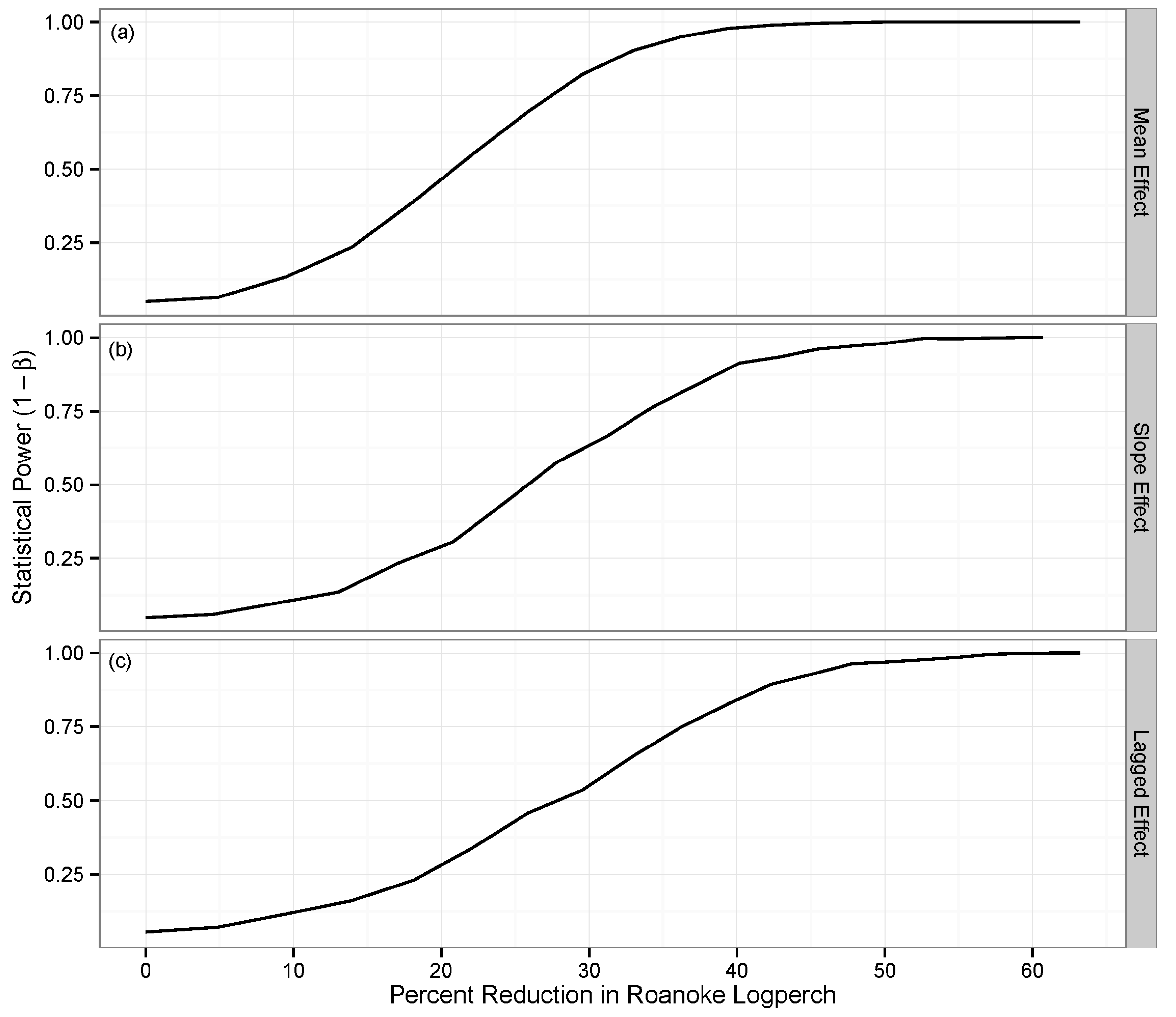
Step 6. Design monitoring studies (including spatiotemporal attributes and analytical tools) capable of testing hypotheses.Available resources (i.e., time and money) may be severely limiting.
Allocate enough spatial and temporal replication to characterize mean and variance of indicators in each treatment group and provide adequate statistical power to detect changes of interest, including lagged effects.
For samples of animal abundance, account for imperfect detection.
Monitoring studies that cannot provide valid statistical tests of effects of proposed alteration.
Inadequate spatial or temporal replication results in poor estimates of mean and variance and/or low statistical power to detect effects of proposed alteration.
Initial plan for pre-construction phase included a single year of monitoring.
We did not use power analysis to inform the spatiotemporal design of the monitoring program.
Power analysis showed we had low statistical power to detect lagged post-treatment effects.
We conducted capture-recapture studies to estimate logperch detection probability.
Implementation phase
Step 7. Conduct pre-treatment monitoring.Measure all selected indicators and their drivers.
Collect all samples as consistently as possible.
Important indicators and drivers of indicators are not measured and cannot be accounted for when testing hypotheses.Confounding effects of non-RRFRP actions within the catchment.
We accounted for variation in logperch detectability in statistical models.
Environmental and human variability between replicate samples obscures relations among indicators.
Step 8. Re-evaluate conceptual model (see Figure 1b), hypotheses, and monitoring design; revise as appropriate.Use data from pre-treatment monitoring and/or concurrent data collected by others to update knowledge and enhance monitoring effectiveness.Best available knowledge is not applied to monitoring effort; monitoring effectiveness is compromised.Knowledge gained during pre-treatment monitoring was used to a) add young-of-year monitoring and b) revise the logperch-abundance “trigger” that indicated excessive take.
Step 9. Implement proposed alteration and conduct post-treatment monitoring.Same as Step 7.Same as Step 7.Same as Step 7.
Step 10. Test hypotheses using appropriate analytical tools, then draw inferences and conclusions.Examine and account for covariates, indirect relations, and autocorrelation when testing hypotheses.
Use statistical effect sizes to evaluate change in indicators vis a vis desired or acceptable endpoints.
Failure to account for covariates, indirect relations, and autocorrelation obscures relations between alteration and indicators.
Use of simple statistical significance thresholds (e.g., p < 0.05) provides hypothesis-test results with no clear biological interpretation.
Statistical models accounted for effects of logperch detectability and spatiotemporal autocorrelation but did not account for other potential influences on adult abundance.
We based conclusions about project impacts on the magnitude and direction of effect sizes for various hypothesized RRFRP-related effects.
Step 11. Revise conceptual model (see Figure 1b) and evaluate monitoring methods based on results.Build an adaptive management approach into the project.Administrative, regulatory, and/or funding limitations may preclude changes to the monitoring program after it begins.Some flexibility to alter monitoring and analyses emerged but was not planned at the outset; the basic spatiotemporal scope and main methods used were not adaptive.
Communication phase
Step 12. Communicate results to stakeholders and articulate applications for future projects.Communication with stakeholders and application of new knowledge more effective if communication occurs continually rather than sporadically or simply when monitoring is completed.Stakeholders who have use or need of new knowledge do not have timely access to it.As findings emerged, our communication with state and federal managers of logperch led to changes in their management tactics and priorities for research to inform logperch conservation.
Table 2. Considerations in the use of a Before-After-Control-Impact (BACI) design to measure ecological responses to impacts or restoration activities in rivers. Table entries emerged from our experiences in the Roanoke River Flood Reduction Project. “ANOVA” refers to analysis of variance; “GLMM” refers to generalized linear mixed model.
BACI AssumptionPotential Reasons for ViolationPotential Consequences of ViolationPotential Solutions
Treatment occurs instantly at the B-A transition and then is applied uniformly to I sites, throughout the A period.Proposed alteration does not occur all at once, resulting in spatiotemporal variation in project effects.Increased spatial and temporal variance in A-I replicate samples; Some A-I replicates do not accurately characterize treatment effects; Cumulative effects of project are underestimated.Only assign those sites receiving the treatment to the I group; Use regression-based models that allow treatment effect size to vary.
Indicator variables respond instantly at the B-A transition, via a change in their means.Biological/ecological responses are immediate, but responses are not observable in indicator variables until well into the A period.Early A-I replicate samples do not accurately characterize treatment effects; Statistical power to detect change is reduced.Measure indicator variables most likely to detect change (e.g., juvenile logperch abundance); Develop a set of competing a priori hypotheses representing different functional forms of response in indicator variables;
In this case, anticipate a lagged observed response and allocate replicate A-I samples to appropriate treatment groups.
Indicator variables exhibit a lagged response, once a critical threshold of cumulative environmental change is reachedEarly A-I replicate samples do not accurately characterize treatment effects; Statistical power to detect change is reducedMeasure indicator variables most likely to detect change (e.g., habitat); Develop a set of competing a priori hypotheses representing different functional forms of response in indicator variables; In this case, anticipate a lagged observed response and allocate replicate A-I samples to appropriate treatment groups.
Indicator variables respond via a gradual change, due to chronic effects (i.e., “press” disturbance).ANOVA-type tests for change in mean values (intercepts) are inappropriate and underestimate ultimate changes.Develop a set of competing a priori hypotheses representing different functional forms of response in indicator variables; In this case, anticipate a change in the temporal slope (not intercept) of the indicator variable; Utilize regression-based models.
All measured differences between B-A and C-I are due to the project.Other environmental variables change over space and time.Depending on the spatial and temporal distribution of extrinsic influences, these may bias statistical tests toward or away from detecting effects; They likely will reduce precision as well, reducing the probability of detecting real effects.To the extent possible, either control or block for extrinsic sources of variability; For other sources, incorporate them into models as random effects or covariates.
Indicator variables are measured without error.Sampling sites do not represent area-wide conditions.Measured variation in indicators within sample sites does not reflect biological/ecological trends across the study area.Randomize site selection; Use GLMMs to account for random effects of sites when partitioning sources of variation.
Environmental and investigator variability over space and time introduces measurement error.Depending on the spatial and temporal distribution of these influences, they may bias statistical tests toward or away from detecting effects; They likely will reduce precision as well, reducing the probability of detecting real effects.Use repeated-sampling methods (e.g., occupancy or mark-recapture models) to reduce influences of observation/measurement error on estimates of indicators.
Treatment has no effect on C sites.Environmental effects of treatment are transmitted beyond the I area.A-C sites do not accurately represent the reference condition; Statistical power to detect change is reduced; Ultimate effects of the project are underestimated.Select C and I sites that are as environmentally correlated as possible, but where C sites are not affected by the treatment being applied to I.
C and I sites may be demographically interdependent.A-C sites do not accurately characterize reference conditions; Statistical power to detect change is reduced; Ultimate effects of the project are underestimated.Select C and I sites that are as environmentally correlated as possible, but where C and I sites are not demographically interdependent on each other.
B and A periods are long enough to accurately represent background (interannual) mean and variance of indicator variables and statistically detect the desired effect size with the desired level of power.Project timeline is short, monitoring resources are limited, temporal variance is higher than expected, or no power analysis has been conducted.Tests have insufficient power to detect the desired effect size with the desired level of power; Ultimate effects of the project are underestimated; Biological/ecological meaning of monitoring results are unclear.Conduct preliminary sampling to estimate mean and variance of indicators, then use power analyses to determine necessary spatial and temporal replication; Allow sufficient pre- and post- time to collect data necessary to assess change.
C and I sites are numerous enough to accurately represent mean and variance of these groups and statistically detect the desired effect size with the desired level of power.Monitoring resources are limited, spatial variance is higher than expected, few replicate habitats are available, or no power analysis has been conducted.Tests have insufficient power to detect the desired effect size with the desired level of power; Ultimate effects of the project are underestimated; Biological/ecological meaning of the monitoring results are unclear.Conduct preliminary sampling to estimate the mean and variance of indicator, then use power analyses to determine necessary spatial and temporal replication; Allow sufficient pre- and post- time to collect data necessary to assess change.

