
Estimation of Polder Retention Capacity Based on ASTER, SRTM and LIDAR DEMs: The Case of Majdany Polder (West Poland)


Abstract
:1. Introduction
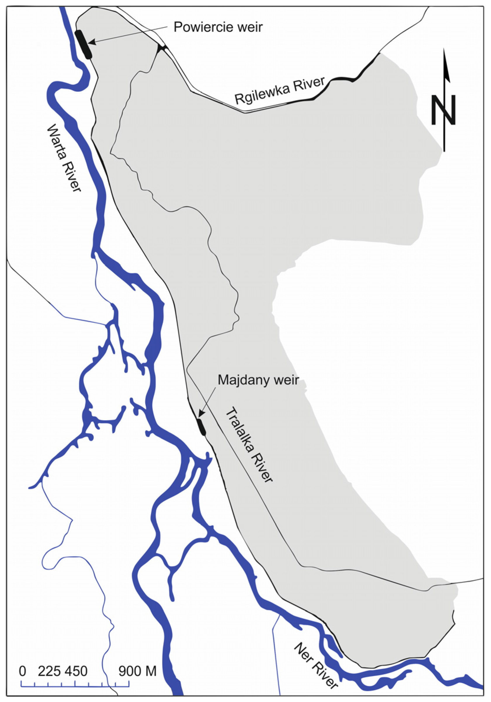
2. Study Area
3. Methodology
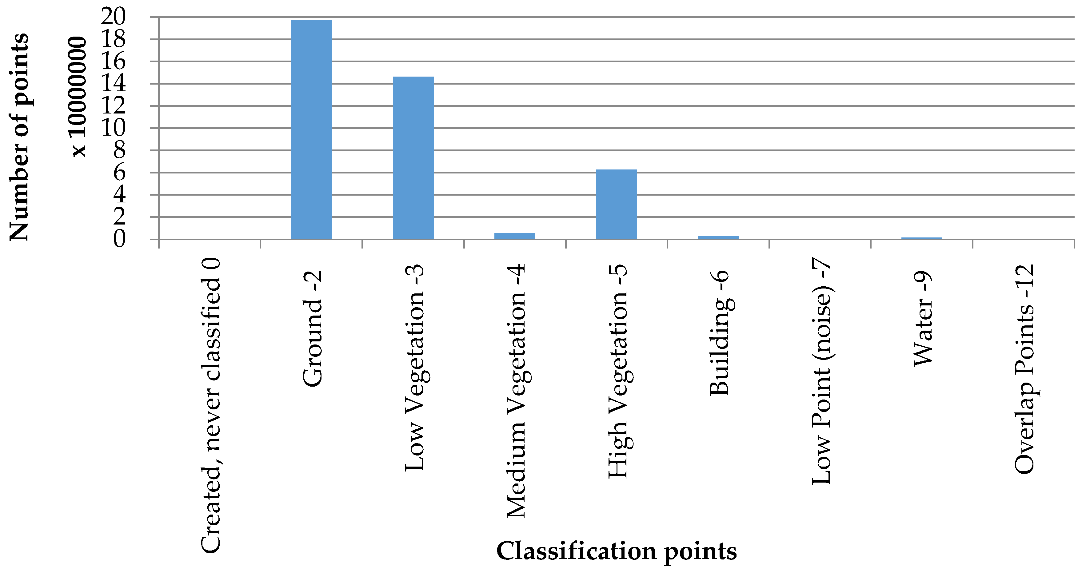
3.1. LIDAR Data
3.2. ASTER and SRTM Data
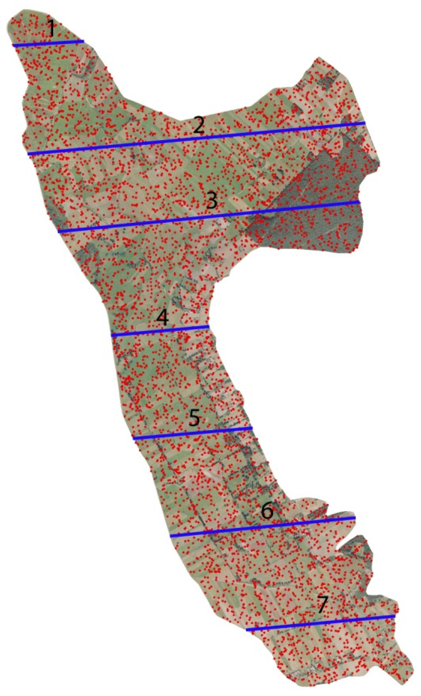
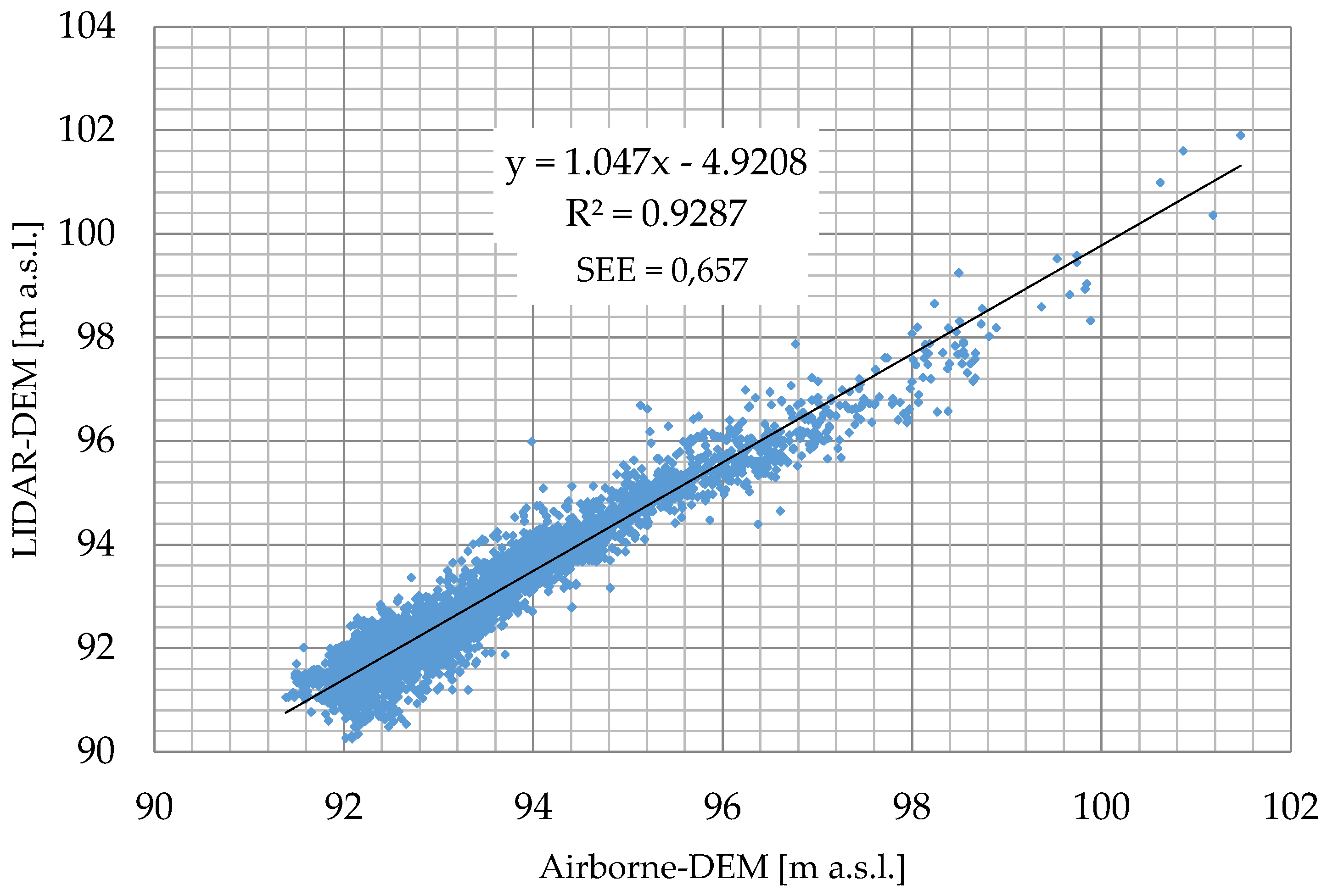
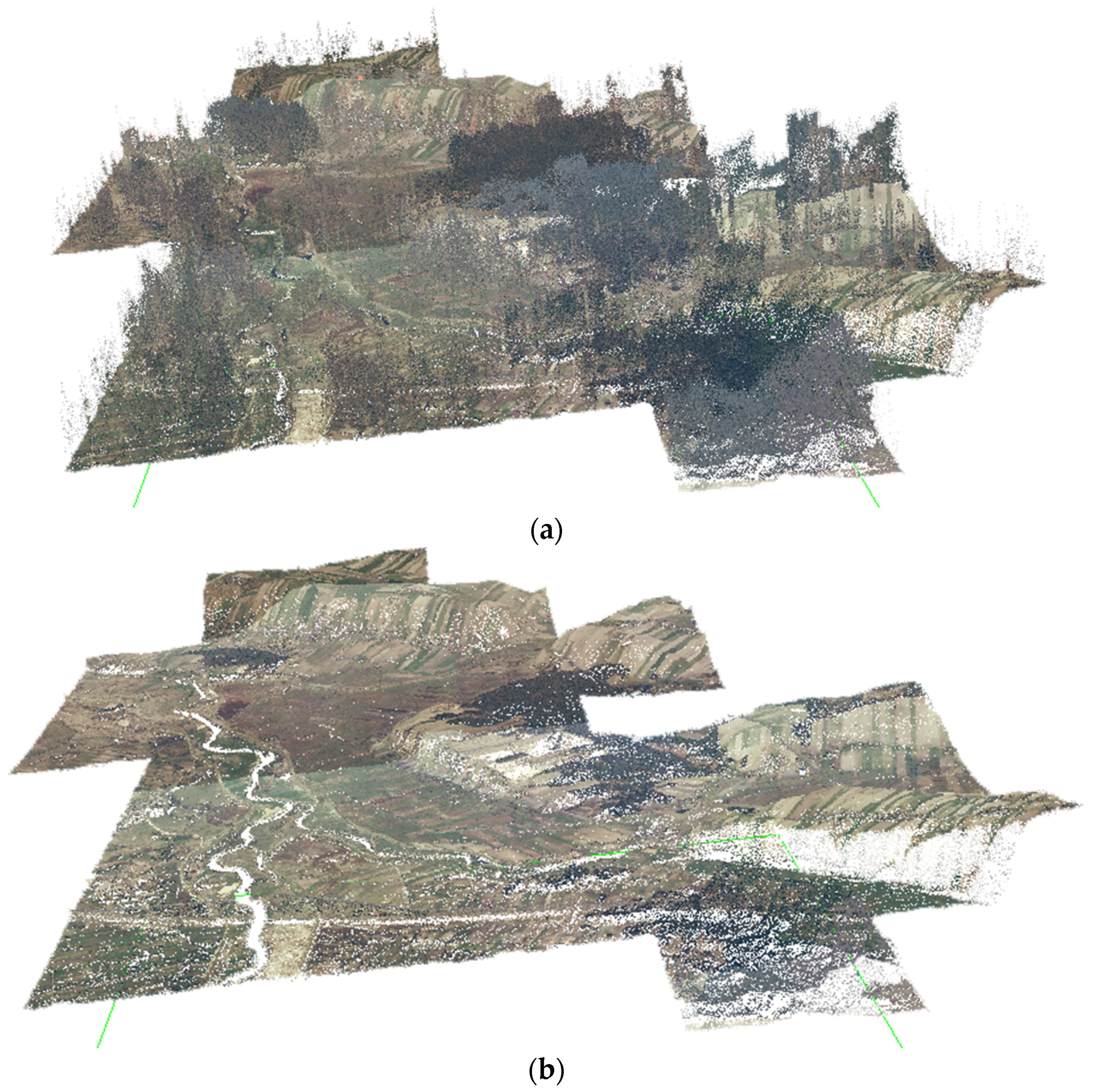
3.3. Airborne Data
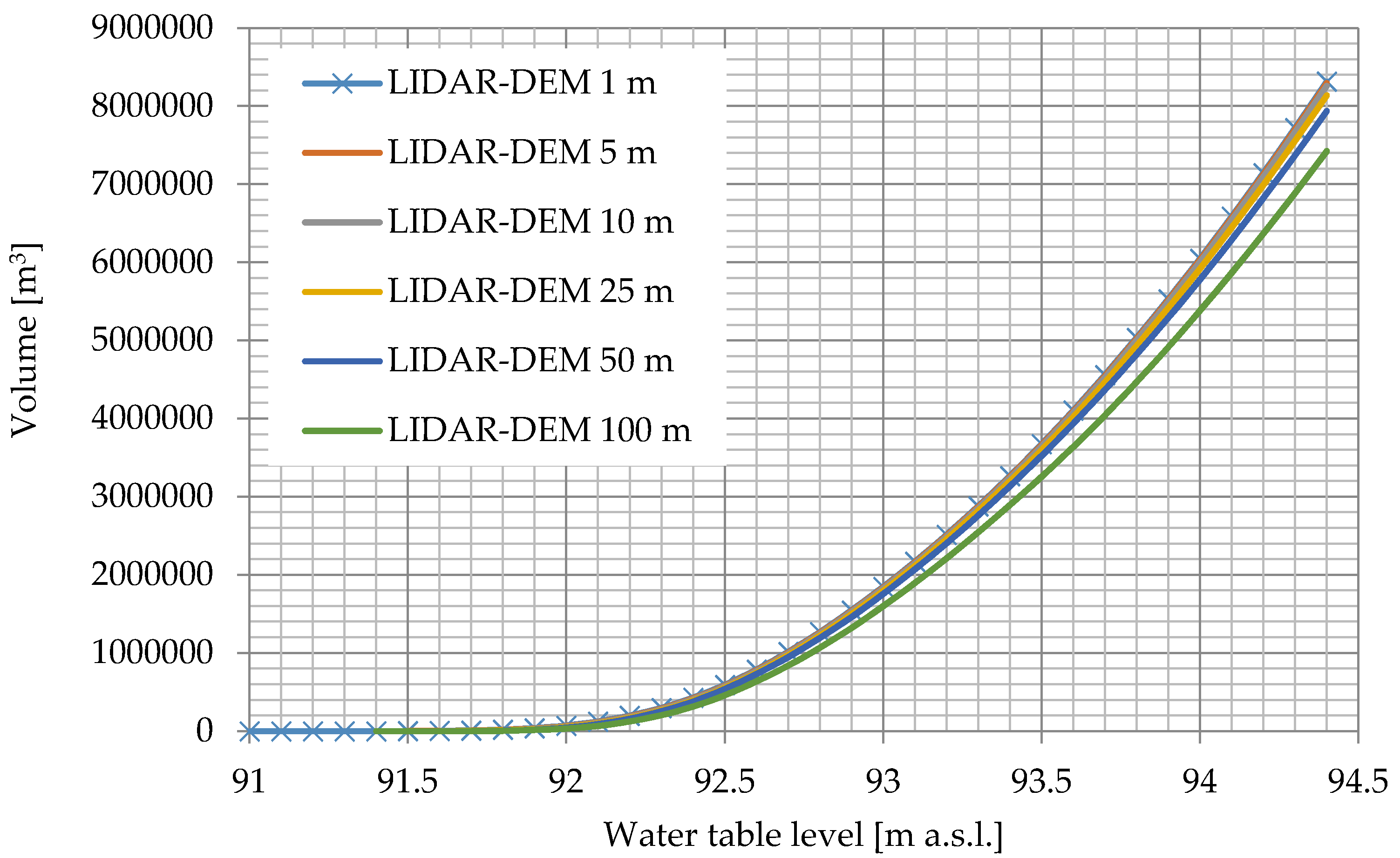
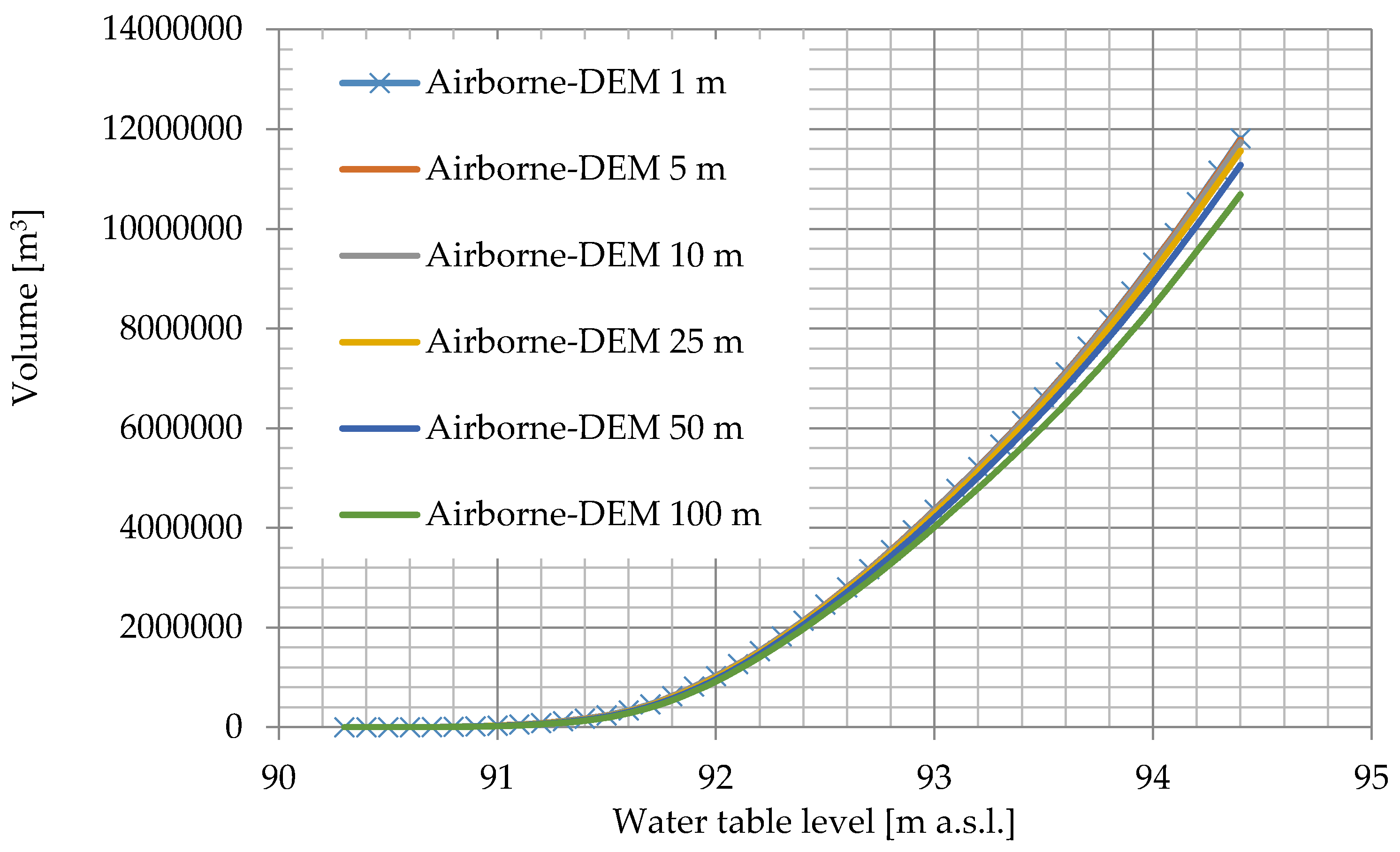
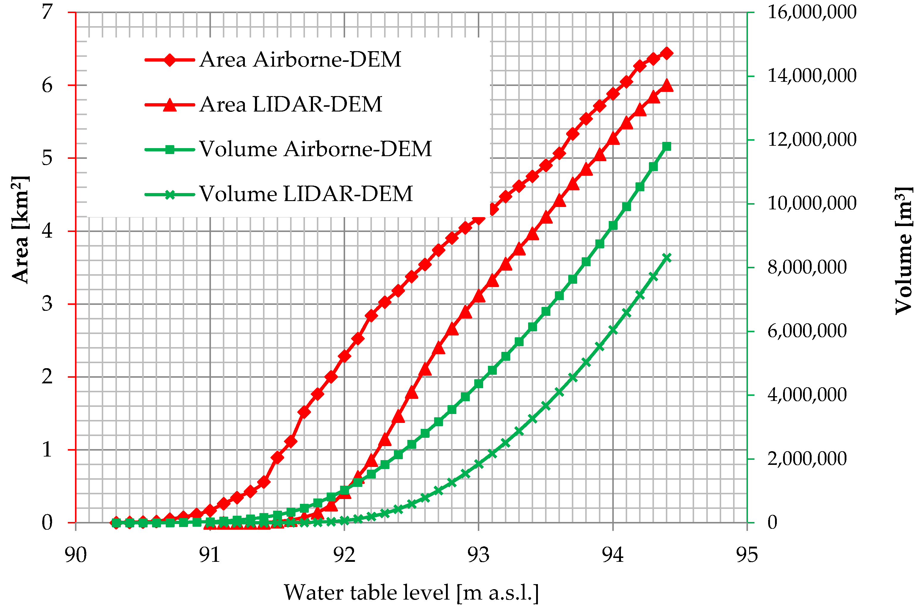
3.4. DEM Resampling and Volume Calculation
4. Results
5. Discussion
6. Conclusions
Acknowledgments
Author Contributions
Conflicts of Interest
References
- Banasiak, R. Use of GIS technics and numerical hydrodynamic models for flood hazard assessment. Infrastrukt. I Ekol. Teren. Wiej. 2012, 3, 123–134. (In Polish) [Google Scholar]
- Teng, J.; Vaze, J.; Dutta, D.; Marvanek, S. Rapid Inundation Modelling in Large Floodplains Using LiDAR DEM. Water Resour. Manag. 2015, 29, 2619–2636. [Google Scholar] [CrossRef]
- Costabile, P.; Macchione, F.; Natale, L.; Petaccia, G. Flood mapping using LIDAR DEM. Limitations of the 1-D modeling highlighted by the 2-D approach. Nat. Hazards 2015, 77, 181–204. [Google Scholar] [CrossRef]
- Schellekens, J.; Brolsma, R.J.; Dahm, R.J.; Donchyts, G.V.; Winsemius, H.C. Rapid setup of hydrological and hydraulic models using OpenStreetMap and the SRTM derived digital elevation model. Environ. Model. Softw. 2014, 61, 98–105. [Google Scholar] [CrossRef]
- Sanecki, J.; Pabisiak, P.; Bauer, R.; Ptak, A.; Stępień, G. The application of DEM and DSM in analysis of flood areas. Folia Sci. Univ. Tech. Resoviensis 2012, 59, 287–293. [Google Scholar]
- Bouwer, L.; Bubeck, P.; Wagtendonk, A.; Aerts, J. Inundation scenarios for flood damage evaluation in polder areas. Nat. Hazards Earth Syst. Sci. 2009, 9, 1995–2007. [Google Scholar] [CrossRef] [Green Version]
- Laks, I.; Kałuża, T. Influence of Konin-Pyzdry valley and Golina polder on flow routing in the Warta river. Zesz. Naukowe Akad. Rol. We Wroc. Inzynieria Srodowiska 2006, 15, 175–183. [Google Scholar]
- Przybyła, C.; Bykowski, J.; Mrozik, K.; Napierała, M. The role of Zagorow polder in flood protection. Rocz. Ochr. Środowiska Sel. Full Texts 2011, 13, 801–813. [Google Scholar]
- Wit, M. Depression of the flood wave culmination by the use of the Smolice polder to protect the town Cracow againts the flood. Gospod. Wodn. 1999, 3, 98–100. (In Polish) [Google Scholar]
- Laks, I.; Kałuża, T.; Sojka, M.; Walczak, Z.; Wróżyński, R. Problems with modelling water distribution in open channels with hydraulic engineering structures. Annu. Set Environ. Prot. 2013, 15, 245–257. [Google Scholar]
- Kowalik, P. Flood control in the Vistula river delta (Poland). Environ. Biotechnol. 2008, 4, 1–6. [Google Scholar]
- Gichamo, T.Z.; Popescu, I.; Jonoski, A.; Solomatine, D. River cross-section extraction from the ASTER global DEM for flood modeling. Environ. Model. Softw. 2012, 31, 37–46. [Google Scholar] [CrossRef]
- Tarekegn, T.H.; Haile, A.T.; Rientjes, T.; Reggiani, P.; Alkema, D. Assessment of an ASTER-generated DEM for 2D hydrodynamic flood modeling. Int. J. Appl. Earth Obs. Geoinform. 2010, 12, 457–465. [Google Scholar] [CrossRef]
- Forkuo, E.K. Flood hazard mapping using Aster image data with GIS. Int. J. Geomat. Geosci. 2011, 1, 932–950. [Google Scholar]
- Schumann, G.; Matgen, P.; Cutler, M.E.J.; Black, A.; Hoffmann, L.; Pfister, L. Comparison of remotely sensed water stages from LiDAR, topographic contours and SRTM. ISPRS J. Photogramm. Remote Sens. 2008, 63, 283–296. [Google Scholar] [CrossRef]
- Ludwig, R.; Schneider, P. Validation of digital elevation models from SRTM X-SAR for applications in hydrologic modeling. ISPRS J. Photogramm. Remote Sens. 2006, 60, 339–358. [Google Scholar] [CrossRef]
- Patro, S.; Chatterjee, C.; Mohanty, S.; Singh, R.; Raghuwanshi, N. Flood inundation modeling using MIKE FLOOD and remote sensing data. J. Indian Soc. Remote Sens. 2009, 37, 107–118. [Google Scholar] [CrossRef]
- Hejmanowska, B. Influence of data quality on modeling of flood zones. Pol. Ttowarzystwo Inf. Przestrz. Rocz. Gematyki 2006, IV, 145–152. [Google Scholar]
- Hejmanowska, B. NMT (GRID/TIN) analysis-Oki data example. Arch. Fotografi-Metrii Kartogr. I Teledetekcji 2007, 17, 281–289. [Google Scholar]
- Hejmanowska, B.; Drzewiecki, W.; Kulesza, Ł. The quality of digital terrain models. Arch. Fotogram. Kartogr. I Teledetekcji 2008, 18, 163–176. [Google Scholar]
- Wang, X.; Lin, Q. Effect of DEM mesh size on AnnAGNPS simulation and slope correction. Environ. Monit. Assess. 2011, 179, 267–277. [Google Scholar] [CrossRef] [PubMed]
- Cook, A.; Merwade, V. Effect of topographic data, geometric configuration and modeling approach on flood inundation mapping. J. Hydrol. 2009, 377, 131–142. [Google Scholar] [CrossRef]
- Pramanik, N.; Panda, R.; Sen, D. One Dimensional Hydrodynamic Modeling of River Flow Using DEM Extracted River Cross-sections. Water Resour. Manag. 2010, 24, 835–852. [Google Scholar] [CrossRef]
- Zhao, Z.; Benoy, G.; Chow, T.; Rees, H.; Daigle, J.-L.; Meng, F.-R. Impacts of Accuracy and Resolution of Conventional and LiDAR Based DEMs on Parameters Used in Hydrologic Modeling. Water Resour. Manag. 2010, 24, 1363–1380. [Google Scholar] [CrossRef]
- Walczak, Z.; Sojka, M.; Laks, I. Assessment of mapping of embankments and control structure on digital elevation model based up on Majdany polder. Ann. Set Environ. Prot. 2013, 15, 2711–2724. [Google Scholar]
- Merwade, V.; Cook, A.; Coonrod, J. GIS techniques for creating river terrain models for hydrodynamic modeling and flood inundation mapping. Environ. Model. Softw. 2008, 23, 1300–1311. [Google Scholar] [CrossRef]
- Liro, A. Strategia Wdrażania Krajowej Sieci Ekologicznej ECONET-Polska; Fundacja IUCN: Warszawa, Poland, 1998. [Google Scholar]
- BirdLife.org. Avaliable online: http://www.birdlife.org/datazone/sitefactsheet.php?id=926 (accessed on 25 May 2016).
- Rozporządzenie Ministra Ochrony Środowiska, Zasobów Naturalnych i Leśnictwa z dnia 20 kwietnia 2007 r. w sprawie warunków technicznych, jakim powinny odpowiadać obiekty budowlane gospodarki wodnej i ich usytuowanie. Dz.U. 2007 nr 86 poz. 579. 2007.
- ISOK. IT system of the Country’s Protection Against Extreme Harazds (ISOK). Avaliable online: http://www.isok.gov.pl/en/ (accessed on 25 May 2016).
- Hladik, C.; Alber, M. Accuracy assessment and correction of a LIDAR-derived salt marsh digital elevation model. Remote Sens. Environ. 2012, 121, 224–235. [Google Scholar] [CrossRef]
- Vaze, J.; Teng, J.; Spencer, G. Impact of DEM accuracy and resolution on topographic indices. Environ. Model. Softw. 2010, 25, 1086–1098. [Google Scholar] [CrossRef]
- Hodgson, M.E.; Bresnahan, P. Accuracy of airborne lidar-derived elevation: Empirical assessment and error budget. Photogramm. Eng. Remote Sens. 2004, 70, 331–340. [Google Scholar] [CrossRef]
- Liu, X. Airborne LiDAR for DEM generation: Some critical issues. Prog. Phys. Geogr. 2008, 32, 31–49. [Google Scholar]
- Grohmann, C.H.; Sawakuchi, A.O. Influence of cell size on volume calculation using digital terrain models: A case of coastal dune fields. Geomorphology 2013, 180–181, 130–136. [Google Scholar] [CrossRef]
- Anderson, E.S.; Thompson, J.A.; Crouse, D.A.; Austin, R.E. Horizontal resolution and data density effects on remotely sensed LIDAR-based DEM. Geoderma 2006, 132, 406–415. [Google Scholar] [CrossRef]
- Zhang, K.; Chen, S.-C.; Whitman, D.; Shyu, M.-L.; Yan, J.; Zhang, C. A progressive morphological filter for removing nonground measurements from airborne LIDAR data. Geosci. Remote Sens. 2003, 41, 872–882. [Google Scholar] [CrossRef]
- Cobby, D.M.; Mason, D.C.; Davenport, I.J. Image processing of airborne scanning laser altimetry data for improved river flood modelling. ISPRS J. Photogramm. Remote Sens. 2001, 56, 121–138. [Google Scholar] [CrossRef]
- Meng, X.; Currit, N.; Zhao, K. Ground filtering algorithms for airborne LiDAR data: A review of critical issues. Remote Sens. 2010, 2, 833–860. [Google Scholar] [CrossRef]
- Zhang, K.; Whitman, D. Comparison of three algorithms for filtering airborne lidar data. Photogramm. Eng. Remote Sens. 2005, 71, 313–324. [Google Scholar] [CrossRef]
- Farr, T.G.; Rosen, P.A.; Caro, E.; Crippen, R.; Duren, R.; Hensley, S.; Kobrick, M.; Paller, M.; Rodriguez, E.; Roth, L. The shuttle radar topography mission. Rev. Geophys. 2007, 45. [Google Scholar] [CrossRef]
- Rodriguez, E.; Morris, C.S.; Belz, J.E. A global assessment of the SRTM performance. Photogramm. Eng. Remote Sens. 2006, 72, 249–260. [Google Scholar] [CrossRef]
- Karwel, A.K.; Ewiak, I. Estimation of the accuracy of the SRTM terrain model in Poland. Arch. Fotogram. Kartogr. I Teledetekcji 2006, 16, 289–296. (In Polish) [Google Scholar] [CrossRef]
- Karwel, A.K.; Ewiak, I. Assessment of useufulness of SRTM data for generation of DEM of the territory of Poland. Pr. Inst. Geod. I Kartogr. 2006, 52, 75–87. (In Polish) [Google Scholar]
- Hofton, M.; Dubayah, R.; Blair, J.B.; Rabine, D. Validation of SRTM elevations over vegetated and non-vegetated terrain using medium footprint lidar. Photogramm. Eng. Remote Sens. 2006, 72, 279–285. [Google Scholar] [CrossRef]
- Jarvis, A.; Rubiano, J.; Nelson, A.; Farrow, A.; Mulligan, M. Practical use of SRTM data in the tropics: Comparisons with digital elevation models generated from cartographic data. Work. Doc. 2004, 198, 32. [Google Scholar]
- Abrams, M. The Advanced Spaceborne Thermal Emission and Reflection Radiometer (ASTER): Data products for the high spatial resolution imager on NASA's Terra platform. Int. J. Remote Sens. 2000, 21, 847–859. [Google Scholar] [CrossRef]
- Cuartero, A.; Felicísimo, A.; Ariza, F. Accuracy of DEM generation from Terra-Aster stereo data. Int. Arch. Photogramm. Remote Sens. 2004, 35, 559–563. [Google Scholar]
- Hirano, A.; Welch, R.; Lang, H. Mapping from ASTER stereo image data: DEM validation and accuracy assessment. ISPRS J. Photogramm. Remote Sens. 2003, 57, 356–370. [Google Scholar] [CrossRef]
- Yamaguchi, Y.; Kahle, A.B.; Tsu, H.; Kawakami, T.; Pniel, M. Overview of advanced spaceborne thermal emission and reflection radiometer (ASTER). Geosci. Remote Sens. 1998, 36, 1062–1071. [Google Scholar] [CrossRef]
- Lewiński, S.; Ewiak, I. Preliminary assessment of usefulness of ASTER satellite images in remote sensing and photogrammetry. Arch. Fotogra. Kartogr. I Teledetekcji 2004, 14, 369–380. (In Polish) [Google Scholar]
- Przybyła, C.; Pyszny, K. Comparison of Digital Elevation Models SRTM and ASTER GDEM and evaluation of the possibility of their use in hydrological modeling in areas of low drop. Ann. Set Environ. Prot. 2013, 15, 1489–1510. [Google Scholar]
- Nikolakopoulos, K.G.; Kamaratakis, E.K.; Chrysoulakis, N. SRTM vs. ASTER elevation products. Comparison for two regions in Crete, Greece. Int. J. Remote Sens. 2006, 27, 4819–4838. [Google Scholar] [CrossRef]
- Forkuor, G.; Maathuis, B. Comparison of SRTM and ASTER Derived Digital Elevation Models over Two Regions in Ghana–Implications for Hydrological and Environmental Modeling. Stud. Environ. Appl. Geomorphol. 2012, 219–240. [Google Scholar] [CrossRef]
- Slater, J.A.; Heady, B.; Kroenung, G.; Curtis, W.; Haase, J.; Hoegemann, D.; Shockley, C.; Tracy, K. Evaluation of the New ASTER Global Digital Elevation Model; National Geospatial-Intelligence Agency: Springfield, VA, USA, 2009. Avaliable online: http://earth-info.nga.mil/GandG/elevation/ (accessed on 25 May 2016).
- Huggel, C.; Schneider, D.; Miranda, P.J.; Delgado Granados, H.; Kääb, A. Evaluation of ASTER and SRTM DEM data for lahar modeling: A case study on lahars from Popocatépetl Volcano, Mexico. J. Volcanol. Geotherm. Res. 2008, 170, 99–110. [Google Scholar] [CrossRef] [Green Version]
- Athmania, D.; Achour, H. External validation of the ASTER GDEM2, GMTED2010 and CGIAR-CSI-SRTM v4. 1 free access digital elevation models (DEMs) in Tunisia and Algeria. Remote Sens. 2014, 6, 4600–4620. [Google Scholar] [CrossRef]
- Kääb, A. Combination of SRTM3 and repeat ASTER data for deriving alpine glacier flow velocities in the Bhutan Himalaya. Remote Sens. Environ. 2005, 94, 463–474. [Google Scholar] [CrossRef]
- Henry, J.B.; Malet, J.P.; Maquaire, O.; Grussenmeyer, P. The use of small-format and low-altitude aerial photos for the realization of high-resolution DEMs in mountainous areas: Application to the Super-Sauze earthflow (Alpes-de-Haute-Provence, France). Earth Surf. Proc. Land. 2002, 27, 1339–1350. [Google Scholar] [CrossRef] [Green Version]
- Grohmann, C.H.; Smith, M.J.; Riccomini, C. Multiscale analysis of topographic surface roughness in the Midland Valley, Scotland. Geosci. Remote Sens. 2011, 49, 1200–1213. [Google Scholar] [CrossRef]
- Horritt, M.; Bates, P. Effects of spatial resolution on a raster based model of flood flow. J. Hydrol. 2001, 253, 239–249. [Google Scholar] [CrossRef]
- Cotter, A.S.; Chaubey, I.; Costello, T.A.; Soerens, T.S.; Nelson, M.A. Water quality model output uncertainty as affected by spatial resolution of input data. J. Am. Water Resour. Assoc. 2003, 39, 977–986. [Google Scholar] [CrossRef]
- Thomas, J.; Joseph, S.; Thrivikramji, K.P.; Arunkumar, K.S. Sensitivity of digital elevation models: The scenario from two tropical mountain river basins of the Western Ghats, India. Geosci. Front. 2014, 5, 893–909. [Google Scholar] [CrossRef]
- Mondal, A.; Khare, D.; Kundu, S.; Mukherjee, S.; Mukhopadhyay, A.; Mondal, S. Uncertainty of soil erosion modeling using open source high resolution and aggregated DEMs. Geosci. Front. [CrossRef]
- Wang, H.; Ellis, E. Spatial accuracy of orthorectified IKONOS imagery and historical aerial photographs across five sites in China. Int. J. Remote Sens. 2005, 26, 1893–1911. [Google Scholar] [CrossRef]
- Pulighe, G.; Fava, F. DEM extraction from archive aerial photos: Accuracy assessment in areas of complex topography. Eur. J. Remote Sens. 2013, 46, 363–378. [Google Scholar] [CrossRef]
- Mukherjee, S.; Joshi, P.; Mukherjee, S.; Ghosh, A.; Garg, R.; Mukhopadhyay, A. Evaluation of vertical accuracy of open source Digital Elevation Model (DEM). Int. J. Appl. Earth Obs. Geoinform. 2013, 21, 205–217. [Google Scholar] [CrossRef]
- Suwandana, E.; Kawamura, K.; Sakuno, Y.; Kustiyanto, E.; Raharjo, B. Evaluation of ASTER GDEM2 in Comparison with GDEM1, SRTM DEM and Topographic-Map-Derived DEM Using Inundation Area Analysis and RTK-dGPS Data. Remote Sens. 2012, 4, 2419. [Google Scholar] [CrossRef]
- Rexer, M.; Hirt, C. Comparison of free high resolution digital elevation data sets (ASTER GDEM2, SRTM v2. 1/v4. 1) and validation against accurate heights from the Australian National Gravity Database. Aust. J. Earth Sci. 2014, 61, 213–226. [Google Scholar] [CrossRef]
- Li, P.; Shi, C.; Li, Z.; Muller, J.-P.; Drummond, J.; Li, X.; Li, T.; Li, Y.; Liu, J. Evaluation of ASTER GDEM using GPS benchmarks and SRTM in China. Int. J. Remote Sens. 2013, 34, 1744–1771. [Google Scholar] [CrossRef]
- Wang, W.; Yang, X.; Yao, T. Evaluation of ASTER GDEM and SRTM and their suitability in hydraulic modelling of a glacial lake outburst flood in southeast Tibet. Hydrol. Process. 2012, 26, 213–225. [Google Scholar] [CrossRef]
- Kidner, D.B.; Smith, D.H. Advances in the data compression of digital elevation models. Comput. Geosci. 2003, 29, 985–1002. [Google Scholar] [CrossRef]
- Zandbergen, P.A. The effect of cell resolution on depressions in digital elevation models. Appl. GIS 2006, 2, 04.01–04.35. [Google Scholar] [CrossRef]
- Tan, M.L.; Ficklin, D.L.; Dixon, B.; Ibrahim, A.L.; Yusop, Z.; Chaplot, V. Impacts of DEM resolution, source, and resampling technique on SWAT-simulated streamflow. Appl. Geogr. 2015, 63, 357–368. [Google Scholar] [CrossRef]
- Hydroprojekt. Building-Executive Project of “Polder Majdan-Increasing the Ner and Warta River Right-Site Embankment in Dabie”; Hydroprojekt Sp. z o.o.: Poznań, Poland, 2002. [Google Scholar]


| Statistical Measures | |
|---|---|
| Average square error | |
| Average error | |
| Accidental error |
| Error Indicator 1 | Unit | Embankment | |
|---|---|---|---|
| Airborne-DEM | LIDAR-DEM | ||
| Min. | m | −1.86 | −0.33 |
| Max. | m | 1.46 | 0.57 |
| RMSE | m | 0.72 | 0.12 |
| SD | m | 0.57 | 0.11 |
| ME | m | −0.44 | 0.05 |
| Airborne-DEM | ASTER-DEM | SRTM-DEM | |
|---|---|---|---|
| RMSE | 0.657 | 3.973 | 5.399 |
| Studies | Study Areas | ASTER-GDEM2 | SRTM v4.1 | ||
|---|---|---|---|---|---|
| ME | RMSE | ME | RMSE | ||
| Suwandana et al. [68] | Karian Dam, Indonesia | N/A | 5.68 | N/A | 3.25 |
| Rexer and Hirt [69] | Australia (Bare areas) | −4.22 | 8.05 | 2.69 | 3.43 |
| Li et al. [70] | China (Tibetan Plateau) | −5.9 | 14.1 | 0.9 | 8.6 |
| Mukherjee et al. [67] | Shiwalik Himalaya, India | −2.58 | 6.08 | −2.94 | 9.2 |
| Athmania and Achour [57] | Anaguid test site | −2.32 | 5.3 | 0.48 | 3.6 |
| Tebessa test site | −1.02 | 9.8 | 0.48 | 8.3 | |
| Pulighe and Fava [66] | Italy, southern Sardinia | 5.82 | 12.95 | N/A | N/A |
| Wang, et al. [71] | Southeast Tibet | 15.4 | 13.5 | ||
| Forkuor and Maathuis [54] | Ghana Guinea Savannah | −3.30 | 5.46 | 3.67 | 4.95 |
| Ghana Volta Lake | −3.32 | 18.76 | 2.09 | 14.54 | |
| This study | Majadny polder | 2.7 | 3.97 | 0.61 | 5.39 |
© 2016 by the authors; licensee MDPI, Basel, Switzerland. This article is an open access article distributed under the terms and conditions of the Creative Commons Attribution (CC-BY) license (http://creativecommons.org/licenses/by/4.0/).
Share and Cite
Walczak, Z.; Sojka, M.; Wróżyński, R.; Laks, I. Estimation of Polder Retention Capacity Based on ASTER, SRTM and LIDAR DEMs: The Case of Majdany Polder (West Poland). Water 2016, 8, 230. https://doi.org/10.3390/w8060230
Walczak Z, Sojka M, Wróżyński R, Laks I. Estimation of Polder Retention Capacity Based on ASTER, SRTM and LIDAR DEMs: The Case of Majdany Polder (West Poland). Water. 2016; 8(6):230. https://doi.org/10.3390/w8060230
Chicago/Turabian StyleWalczak, Zbigniew, Mariusz Sojka, Rafał Wróżyński, and Ireneusz Laks. 2016. "Estimation of Polder Retention Capacity Based on ASTER, SRTM and LIDAR DEMs: The Case of Majdany Polder (West Poland)" Water 8, no. 6: 230. https://doi.org/10.3390/w8060230