
Bed Evolution under Rapidly Varying Flows by a New Method for Wave Speed Estimation


Department of Civil and Environmental Engineering, Hanyang University, 222 Wangsimni-ro, Seongdong-gu, Seoul 04763, Korea
*
Author to whom correspondence should be addressed.
Water 2016, 8(5), 212; https://doi.org/10.3390/w8050212
Submission received: 9 April 2016
/
Revised: 8 May 2016
/
Accepted: 16 May 2016
/
Published: 20 May 2016
Abstract
:This paper proposes a sediment-transport model based on coupled Saint-Venant and Exner equations. A finite volume method of Godunov type with predictor-corrector steps is used to solve a set of coupled equations. An efficient combination of approximate Riemann solvers is proposed to compute fluxes associated with sediment-laden flow. In addition, a new method is proposed for computing the water depth and velocity values along the shear wave. This method ensures smooth solutions, even for flows with high discontinuities, and on domains with highly distorted grids. The numerical model is tested for channel aggradation on a sloping bottom, dam-break cases at flume-scale and reach-scale with flat bottom configurations and varying downstream water depths. The proposed model is tested for predicting the position of hydraulic jump, wave front propagation, and for predicting magnitude of bed erosion. The comparison between results based on the proposed scheme and analytical, experimental, and published numerical results shows good agreement. Sensitivity analysis shows that the model is computationally efficient and virtually independent of mesh refinement.
1. Introduction
Numerical techniques for modeling morphodynamics are preferable over field and laboratory observations at large scales, due to reduced computational costs and time [1,2,3,4]. Mathematical modeling of morphodynamics can be performed using depth-integrated shallow-water equations (continuity and momentum equations) representing the hydrodynamics, and an Exner equation (continuity of sediment) representing the morphological evolution. These equations can either be modeled using a coupled approach in which the hydrodynamic and morphodynamics flows are solved simultaneously, or using an uncoupled (quasi two-phase) approach, in which flow hydrodynamics are modeled first and then the obtained velocity is used for modeling morphological evolution [5]. According to [6,7], the coupled approach is best suited for analysis of rapidly varying flow conditions, where flow unsteadiness strongly affects sediment evolution; while the uncoupled approach is mostly used for slowly varying flows. The applicability of the uncoupled approach is limited due to the assumption of constant sediment concentration in the lower layer [8].
Coupled shallow-water and Exner equations have been widely used to model sediment transport in rivers, bed evolution in dam-break flows, siltation of reservoirs, and sediment flushing in sewers [4,9,10,11,12,13,14]. In this study, the authors used a coupled model based on approaches adopted by Goutière, Soares-Frazão et al. (2008) and Murillo and García-Navarro (2010) to simulate a bed load sediment-transport initiated by water flow. Different equations are used in the literature to model solid transport sediment flux. Commonly used sediment-transport formulas include the Grass formula [15], Meyer-Peter and Muller’s (MPM) equation [16], Van Rijn’s equation [17,18,19], and Nielsen’s formula [20]. The performance of various transport formulas is reported in [21]. For simplicity, the authors have adopted Grass’s model in this study to define a solid transport discharge. This is a simple sediment formula that combines a global case dependent calibration and an easily differentiable power law of velocity [22].
We use the volume method of Godunov-type to solve coupled shallow-water and Exner equations models. Two approaches are usually employed for the computation of interface fluxes in coupled models, the Roe approximate Riemann solver [5,10,22,23,24,25,26,27], and the Harten-Lax-van Leer-Contact (HLLC) approximate Riemann solver [7,14]. A predictor-corrector step is adopted for evolving the solution to get second-order temporal accuracy. In the predictor step, the solution is updated by half a time step using a non-conservative method; while in the corrector step, the conservation is recovered over a full time step by solving local Riemann problems using the data obtained from the predictor step. The fluxes at the interface are computed using the HLLC approximate Riemann solver for the hydrodynamic part, and by the Harten-Lax-van Leer (HLL) scheme for the morphological changes.
Since this study employs the Riemann problem, the general solution for the hydrodynamic part of the solution consists of three waves, a left and right moving wave and a middle wave (a shear wave). In such a problem, the most important feature of flux computation with the HLLC scheme is the choice of relations for approximating the water depth and velocity along the shear wave. The usual practices of computing these variables are either based on the assumption that the two non-linear waves are either shocks or rarefactions, or by using depth positivity condition (readers are referred to [28] for more details). However, in cases of coupled shallow-water and Exner equations, these equations are not applicable due to differences in wave structure.
Wave speed estimation in HLLC solver requires the values of Roe-averaged states (water depth, velocity, energy states) [29]. These states are obtained from Roe approximations (see details in [30]). Given that the Roe-averaged states are not uniquely defined [31], different approached are adopted for estimating Roe-averaged states. Most of the numerical models for sediment transport studies [6,13,14,22,23] follow Glaister’s approach [32] for computing Roe averages for a coupled shallow-water Exner equations system. However, Hu et al. [33] argued that artificially introduced intermediate states, like that of Glaister’s, may not be admissible for some cases. Therefore, they proposed an extension of the Roe averages for estimation of wave speeds by avoiding artificial states and relying only on intermediate states for state averages.
The HLLC studies [7,14] used the average of left and right Riemann states for computation of variables along the shear wave, but this method makes the solution too dependent on reconstructed values, which can be erroneous for cases in which the grids are skewed or when the problem presents strong discontinuities, and when the reconstruction procedure is not accurate. We propose a new method for approximating the values along the shear wave by Roe averages in which the variable values do not exclusively depend upon reconstructed values. The basic concept is to predict average states directly from the intermediate states by utilizing vertex values at the interface along with reconstructed variables. To make the dependence more even, the variable values at vertex are included in finding the Roe averages. This method avoids potential problems of inaccuracy and instability, which can be caused by meshes with skewed elements, problems with strong discontinuities, and may address the shortcomings of the reconstruction procedure to some extent.
The aim of this work is to develop a simple, but robust, coupled shallow-water flow model that can accurately handle the discontinuities and capture shocks associated with dam-break flows on erodible beds. The objective is to develop a model that can help us study the bed evolution under the sudden release of large volume of water and to accurately capture the wave structure associated with such flows.
2. Governing Equations
The governing equations describe the Saint-Venant system commonly known as shallow-water equations coupled to the Exner equation for sediment-transport and forming a non-linear system of equations.
2.1. Hydrodynamic Component
Flow evolution can be represented by the shallow-water equations. For an inviscid and incompressible flow, these equations can be expressed as:
where t is the time, h is the water depth, u is the velocity component, g is the gravitational acceleration, and S and are the bed slope and bottom frictional terms, respectively, estimated as:
where b is bed elevation, and n is Manning’s roughness coefficient.
2.2. Morphodynamic Component
The sediment dynamics can be expressed by a simple sediment continuity or Exner equation. Mathematically, this equation is given as [12]:
where , p is the sediment porosity and qs is sediment-transport discharge. Physically, Equation (3) implies that time variation of a sediment layer in a control volume is due to the net variation of solid transport through the boundaries of the control volume [22]. In this study, the Exner equation is used in its reduced form, as the main focus is bed evolution and flow dynamics.
A sediment discharge transport formula is used to close Equation (3). To check the performance of the proposed model, we compute bed load discharge using two approaches, the bed load equation of Grass [15] and the MPM sediment transport formula.
2.2.1. Grass Formula
Sediment transport flux in the Grass formula follows a power law, given as:
where A is the intensity of interaction between flow and sediment particles, the value of which ranges between 0 and 1 with increasing interaction strength, and u is the velocity. This equation does not take critical shear stress into account, and it relates the sediment discharge to the flow velocity as in [12]. For the cases modeled in this study, A is either adopted from previous studies, or calculated using Equation (5) for cases with detailed sediment parameters;
where d is the local sediment medium diameter; and ρ are the sediment and water density, respectively; and the particle diameter D* is estimated as
where υ is the kinematic viscosity of water.
2.2.2. MPM Formula
3. Numerical Scheme
In conservative form, Equations (1) and (3) can be written as:
where U is the vector of conserved variables, F is a flux vector functions, and S is a vector of source terms. In vector form, the coupled equations can be written as [13]:
Integration of Equation (9) over the cell gives
where Ω is the volume of a control volume. Equation (11) can be expressed as:
where n denotes the unit outward normal to the boundary of the cell, and F(U)·n is the flux vector normal to the interface, expressed as:
Discretization of Equation (12) takes the form:
where ∆t and ∆x are step sizes in space and time, respectively, and and are the boundaries of the cell. The explicit nature of this scheme demands that the time step is limited by the CFL (Courant-Friedrichs-Lewy coefficient) condition.
where ν is the CFL number, set equal to 0.6 for all cases modeled in this study. Equation (14) is evolved in two steps: the predictor step and the corrector step. In the predictor step, the solution evolves by half a time step employing reconstructed cell center variables. This step is given as:
where and are fluxes at the right and left sides of the cell interface, respectively, n indicates the initial values of variables, and is the vector of conserved variables at the cell center at initial time n. Fluxes are computed by the HLLC and HLL schemes for the hydrodynamic and morphodynamic parts, respectively. The results from Equation (17) are advanced to a full time step in the second stage by the corrector scheme given as:
3.1. Flux Computation
Flux calculation using coupled shallow-water Exner equations is complicated due to the additional wave, related to sediment information in the wave structure. Approximate Riemann solvers (especially Roe and HLLC schemes) can accurately estimate fluxes for shallow-water flows, as these solvers have high resolution and shock capturing capability. However, for cases with strong interface interactions, like dam-break flows over erodible beds, complications arise due to the additional wave (associated with the sediment layer) issued from an initial discontinuity in the coupled equations.
We use HLLC and HLL schemes in this study to compute hydrodynamic and morphological fluxes, respectively. The wave speeds for the coupled system of equations, Equation (7), are estimated from the approximate eigenvalues derived in [13] by analysis of the Jacobian matrix for the coupled system of equations.
where is the wave celerity, and d is a the term involving the normal derivative of sediment transport rate. Differentiating the sediment discharge, given in Equations (4) and (8), gives us:
The largest eigenvalue λ3 accounts for hydrodynamic effects and λ1,2 give eigenvalues carrying sediment characteristic information. The HLLC scheme used for computing hydrodynamic mass and momentum fluxes is given as [34]:
The speed of the middle wave is , and is approximated as
where K = L, R; , , and are variable values along the shear wave estimated by Equations (29) and (30), respectively.
The eigenvalue analysis in [13] shows that sediment flow information (λ1,2) is not affected by the fast moving wave (λ3), since the speed with which sediment information is transmitted is very slow compared to the evolution of other hydrodynamic information. We choose the HLL scheme for computing sediment fluxes because of the constant intermediate state between λ1 and λ2, which is the assumption of HLL scheme. Application of the HLL scheme is simple, as intermediate waves between the slowest and fastest moving waves are not present in this approach. The speed of these waves is estimated by eigenvalues of the coupled equation; the speed of the slowest and fastest travelling waves is estimated by Equation (21). The HLL flux is calculated as [34]:
The important step in arriving at the solution is to approximate the water depth and velocity across the shear wave. Their constant values, in Equations (29) and (30), are computed by a new method in which the contribution of vertex values is also accounted for
where v represents the two vertices of the interface through which the flux is being computed. The vertex values can be computed by the pseudo-Laplacian relation proposed by [35]. This new method for approximation of variable values in the star region also gives weight to the variable values at the vertices. This method is effective for highly skewed control volumes, as well as for structured grids, as the variable approximation does not strongly depend upon the reconstructed values at cell interfaces. In previous studies, the estimation of shear waves is based solely on Roe averages that are obtained by solving locally linearized Riemann problem at each cell interface [12,30,36]:
This method might make the solution susceptible to error for cases in which the mesh is composed of highly distorted grids, which lead to cell-centered variables that are not reconstructed exactly at the mid-point of an interface. We show the performance of the proposed method in Section 3 by modeling various test cases on different meshes.
3.2. Source Term Treatment
Accuracy of the numerical solution is greatly influenced by the source term treatment. In the present study, source terms include variable bed slope and shear stress terms. The scheme is well-balanced if its flux gradient is balanced by the slope source terms for a “lake at rest” condition
where η is water surface elevation. We extend and modify the source term treatment, the revised surface gradient method (RSGM), proposed by [37], for shallow water flows on non-erodible beds. We extend and modify RSGM for erodible beds by introducing reconstructed values of water surface elevation to estimate flow depth average and bed level difference.
The proposed scheme satisfies well-balanced conditions and gives stable and accurate solutions as shown in application of the model. Friction terms were treated explicitly.
3.3. Wetting and Drying
Inaccurate treatment of wetting and drying fronts results in significant errors in solutions, including negative water depths and unphysical high velocities. A simple treatment is adopted in this study, which involves setting a tolerance depth hmin (0.0001 m in our model), below which cells are considered dry, and consequently the momentum flux across the cell interface becomes zero. This treatment of wet-dry fronts is similar to applying solid boundary conditions on the interface between wet and dry cells.
3.4. Boundary Conditions
Wall and open boundary conditions are imposed in the proposed model. Unlike the pure hydrodynamic case, there are three characteristic waves entering and leaving the domain at the inlet and outlet. The additional wave accounts for the presence of sediment. Solid wall conditions are imposed on side walls making the velocity normal to the walls equal to zero. Physical boundary conditions are required at the inlet. For cases in which some physical conditions are not available, the theory of characteristics is used. The inlet boundary conditions are implemented by the same procedure as literature references, including [23,38]. A free outflow condition is imposed at the outlets to enable waves to pass through the boundary without reflection.
4. Applications
4.1. Dam-Break over a Rigid Bed
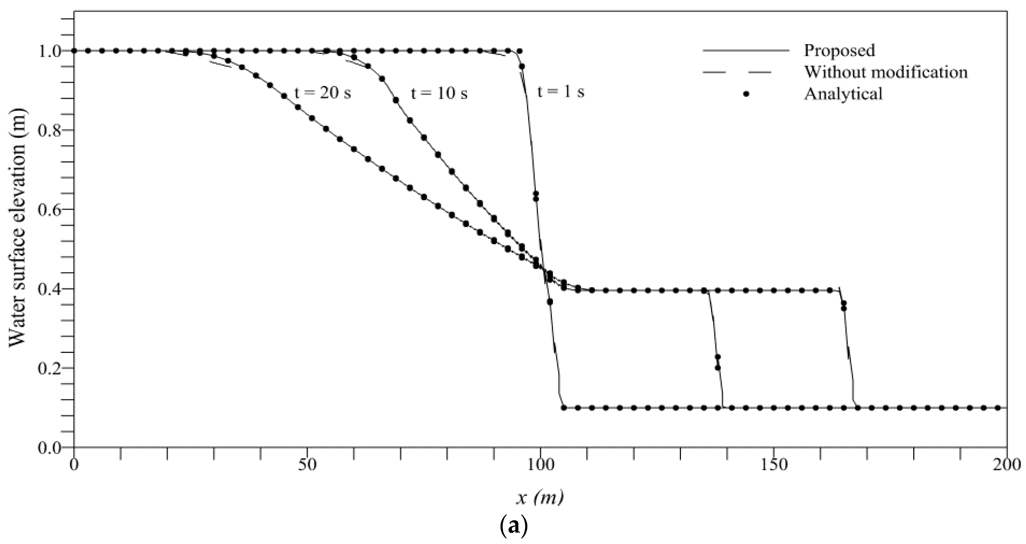
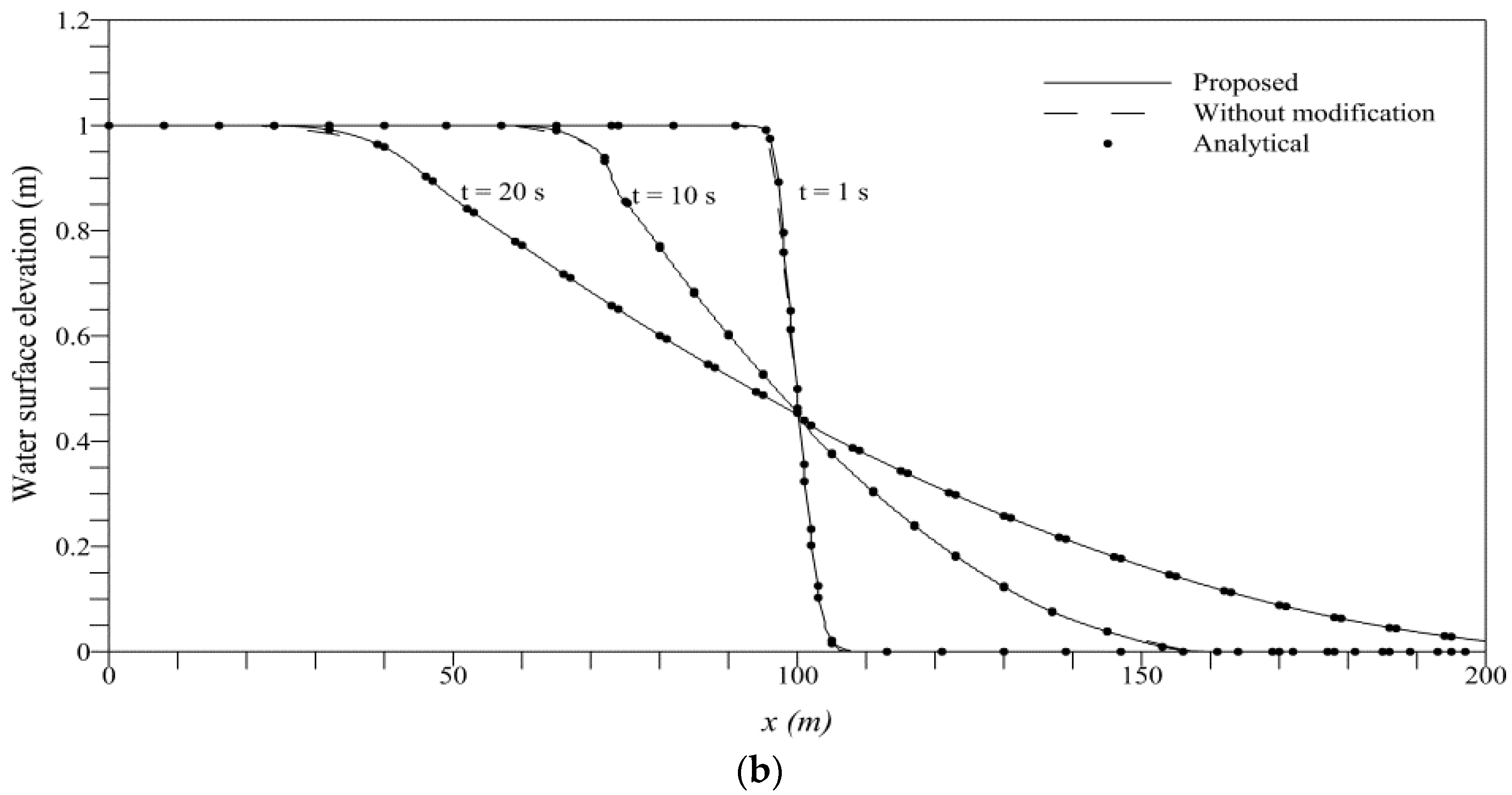
The proposed scheme is first tested for a benchmark hydrodynamic case of dam-break on a rigid non-erodible bed widely employed to verify model’s performance on dry and wet beds. The dam-break is instantaneous on a flat bottom with negligible friction. Based on the water level in the right half of the domain, there are two cases for this problem; if water level is over zero the case is said to be dam-break on a wet domain, and if it is zero the case is dry bed. The initial conditions for this problem constitute a Riemann problem. For initially wet bed the conditions are given as
The initial conditions for dry bed are
where L is the total length of the channel taken equal to 200 m, and is the position of dam. The results are compared with analytical solution [39] at t = 1, 12, 21 and 27 s for flow over wet and bed in Figure 1. The numerical results show excellent agreement with the analytical solution; the transition of wet/dry front is accurately captured showing that the scheme is well-balanced. Proposed solution shows excellent agreement with analytical solution where the results are almost indistinguishable over both wet and dry beds in Figure 1a,b, whereas the scheme without modification also gives very satisfactory predictions with slight difference from the analytical solution when flow changes from subcritical to supercritical; the difference, however, is indistinguishable on the plotted scale. We observe that the water level estimated by proposed scheme gives slightly better results than the scheme without modification.
4.2. Bed-Slope Aggradation
This test case models a sediment-laden flow over a sloping bed that emulates flows in mountainous terrains triggered by torrential rains. A uniform supercritical flow with constant sediment supply enters the domain from the left boundary. Bed evolution is observed until the equilibrium state is reached by gradual aggradation of the bed. Boundary conditions at x = 0 and L are set equal to and 0, respectively. In order to compare our results with [13]—based on similar governing equations to this study—we used the MPM formula to calculate sediment discharge with a mean sediment diameter of 1.65 mm and porosity (p) of 0.42. The analytical solution of this problem was presented by [40], given as:
where denotes the equilibrium state; An is the Fourier Series coefficient, estimated by Equation (39); and is the response time for the problem given as:
The channel characteristics are: length (L) = 6.90 m; width = 0.5 m; bed roughness = 0.0165 s·m−1/3; and slope S0 = 2.4%. The flow parameters are fixed as: water discharge q = 7.98 m3/s and sediment discharge upstream qs = 0.147 m3/s. These parameters give a response time of T0 = 1670 s and a final equilibrium slope, S, equal to 3.03%. The results are compared with the analytical and numerical solution in Figure 2. After start of the flow at t = 0, bed evolution goes through a transient state (observed at t = 900 and 1800 s) until the final equilibrium state is reached at t = 3600 s. Good agreement is observed between the computed and analytical solutions at all time instants. Our scheme gives slightly better approximations for aggradation than the results of [13]. This application shows the applicability of our scheme for modeling sloping rivers. This also demonstrates the capability of the model to compute the equilibrium slope based on aggradation and degradation of channels, which is useful for limiting sedimentation of water bodies.
4.3. Dam-Break in an Erodible Channel
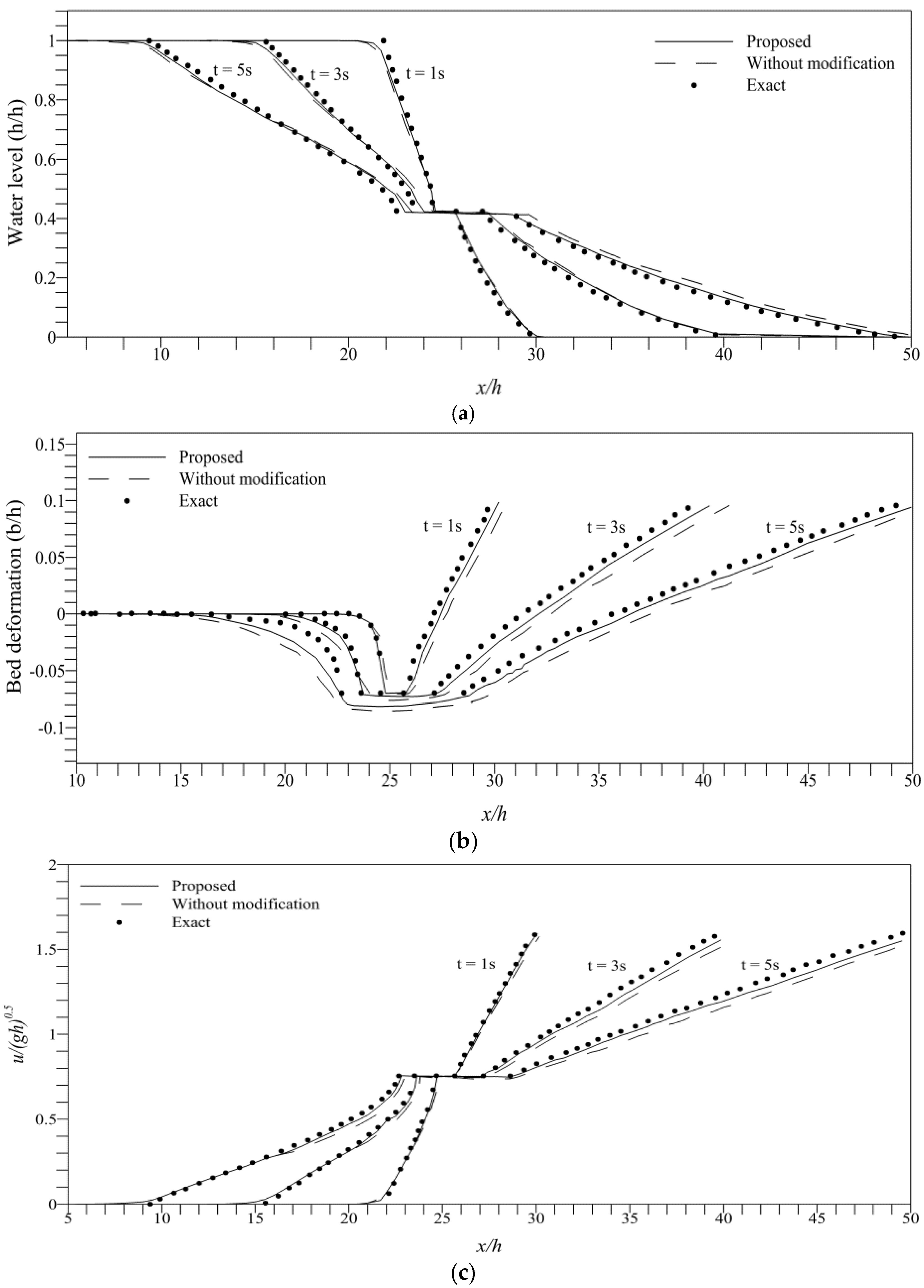
We simulate a dam-break case on a mobile bed to assess the performance of proposed scheme for high speed flows associated with rapid bed deformation and high speed wave propagation. This case was previously also tested by [41,42] to verify their models which were also based on coupled shallow-water and Exner equations.
The computational domain consists of a frictionless erodible channel bed of 50 m length with a dam at the middle of the channel. Following [41,42] the initial water depth of 1 m is fixed upstream of the dam and downstream is considered dry. Computations of sediment discharge by Grass formula and MPM formula have no significant effects on the numerical results for bed evolution, water depths, and velocity [41,42]. We used Grass formula to compute sediment discharge with sediment porosity (p) of 0.4 and A is taken equal to 0.004. At time t = 0, the dam is instantaneously removed; the consequent water level, bed deformation, and velocity is compared with exact Riemann solution of the problem in Figure 3 (readers are referred to [42] for details on exact Riemann solution).
For comparison with the exact solution, the results for water level and bed deformation are non-dimensionalized with respect to initial water depth in the channel, and velocity is non-dimensionalised by wave celerity. The results are plotted at 2 s interval up to 5 s. The numerical results show the correct propagation of wave-front, bed evolution, and velocity. Shocks introduced by the bed discontinuity are well captured at all instants and the numerical solution is free of oscillations. Numerical solution (proposed and without modification) show lag to exact solution at all time instants, which was also observed by [41]. In Figure 3b, we observe that numerical solution slightly overestimates bed deformation with time advancement, which is a characteristic feature of computing sediment discharge by Grass formula due to neglecting water depth in flux estimation. Overall, flow variables show very good agreement with exact solution with the proposed scheme giving better results in all cases.
4.4. Dam-Break over Sand Bed
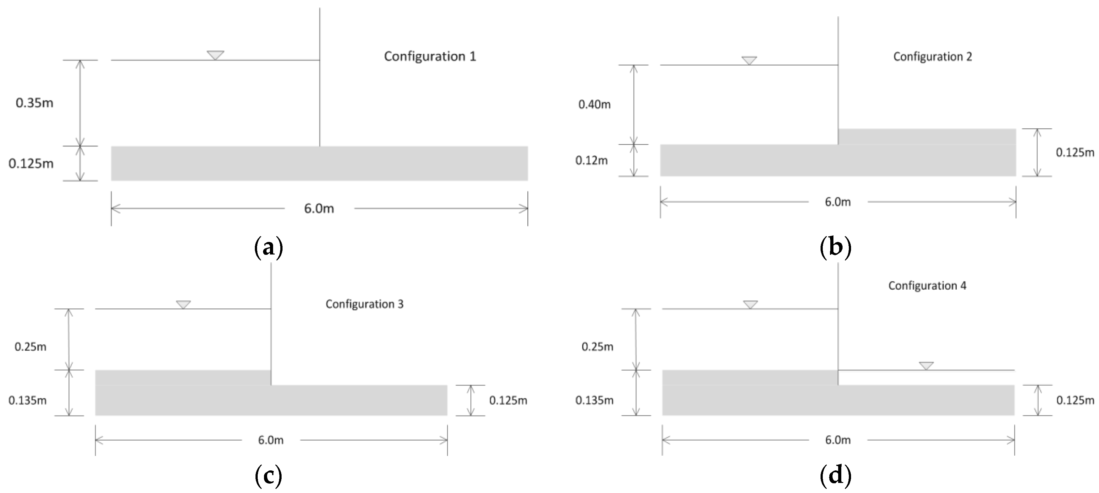
Experimental studies for sand bed evolution under dam-break waves were conducted at the Civil Engineering Department of Universite Catholique de Louvain (UCL), Belgium [43]. The experimental results were later validated by numerical simulations in references [8,22,44,45] as well as by others. The tests were conducted for idealized dam-break cases over an erodible bed. The experimental set-up included a flume 6 m long, 0.25 m wide and 0.70 m deep. A thin steel gate, fixed in the center of flume, was used as a dam in the experiments. In the original experiments [43], the erosion was observed for two bed materials, uniform coarse sand and Polyvinyl Chloride (PVC) pellets. For brevity purposes, this study simulates the experiment with a sand bed, extending on both sides of the dam. The thickness of the sand bed varied for different configurations to account for bed discontinuity at dam location, and these configuration were modeled in the study.
The following [43] four different cases are simulated in this study, which primarily differ in upstream bed layer thickness and initial water depth. Following previous studies [22], the values of the dimensional constant (A), sediment porosity (p), and Manning’s coefficient (n) are set equal to 0.01, 0.4, and 0.0165, respectively, for all configurations. Figure 4 shows the initial configurations for which the dam-break flow is simulated using the proposed scheme. The domain was discretized into 400 cells. The model was run using a refined mesh, but no significant improvement in the results was observed (discussed further in Section 4.5). A CFL number of 0.6 was used due to the explicit nature of the scheme. The dam was removed instantaneously at t = 0, and the results were obtained for the four water surface and bed profiles. Model results were compared to the experimental measurements of Spinewine and Zech (2007) and to the numerical scheme without the modification introduced in Equations (31) and (32).
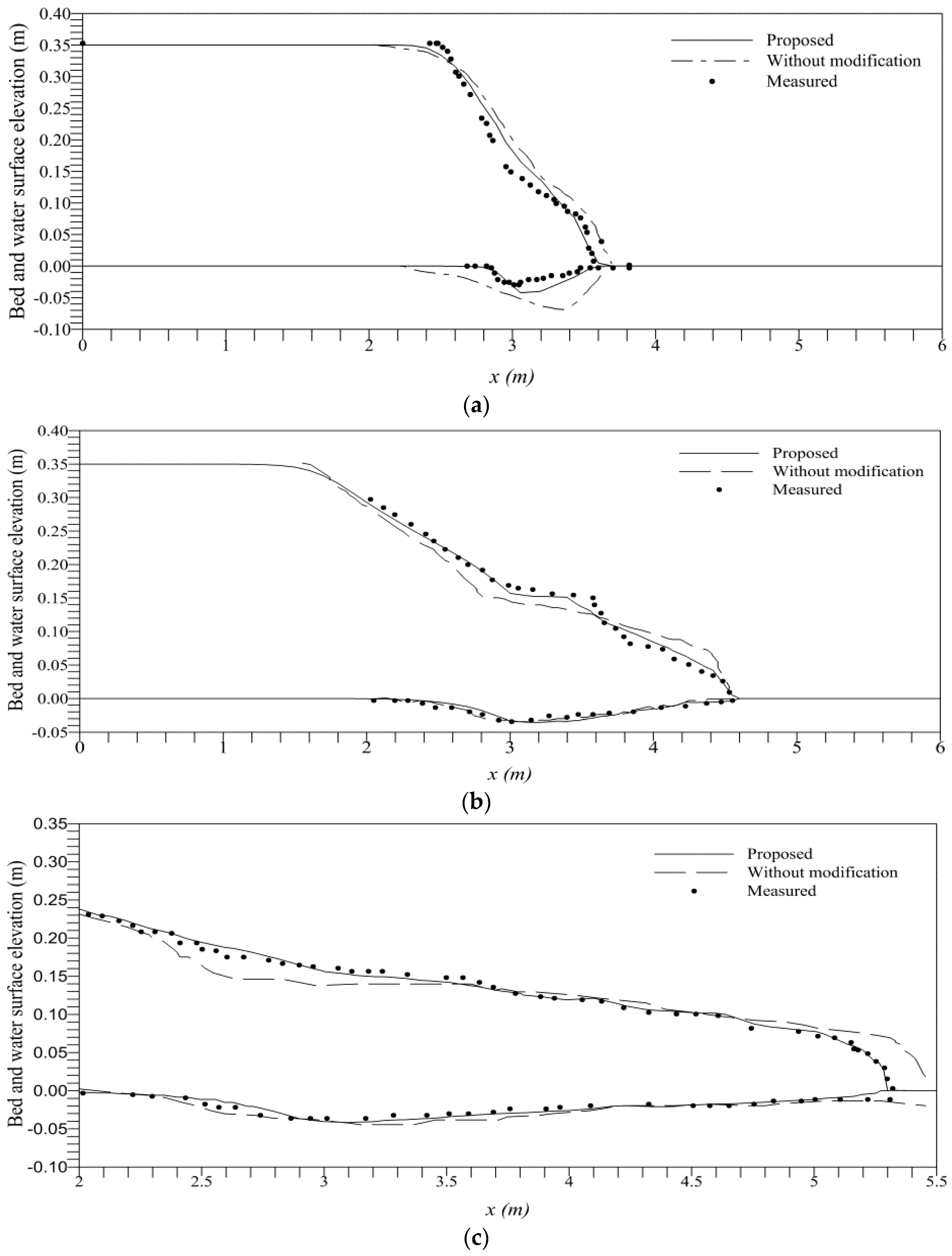
Figure 5, Figure 6, Figure 7 and Figure 8 show the comparisons between the simulated results and experimental measurements. Results for configuration 1 are plotted in Figure 5a–c at 0.25 s, 0.75 s, and 1.25 s, respectively, after the dam-break. At all time intervals, the results using the proposed scheme are in very good agreement with the experimental results. We observe that the model without modification overestimates bed erosion particularly immediately after the dam-break, and is not able to follow the experimental wave-front, whereas the proposed scheme gives very good agreement with the erosion and the wave-fronts observed in the experiment. The position of wave-fronts given by the proposed scheme at t = 0.25 s and 0.75 s are in good agreement with previous results, while at t = 1.25 s it is slightly above the measured, showing slow movement of the wave, due to bed friction. As water propagates downstream, more particles come in contact with the bed surface compared with the initial time intervals resulting in slower propagation of the wave-front. However, considering human error in experimental measurements, and considering the limitations of numerical modeling, we can conclude that, overall, the agreement between numerical results and experimental results using the proposed scheme is very satisfactory.
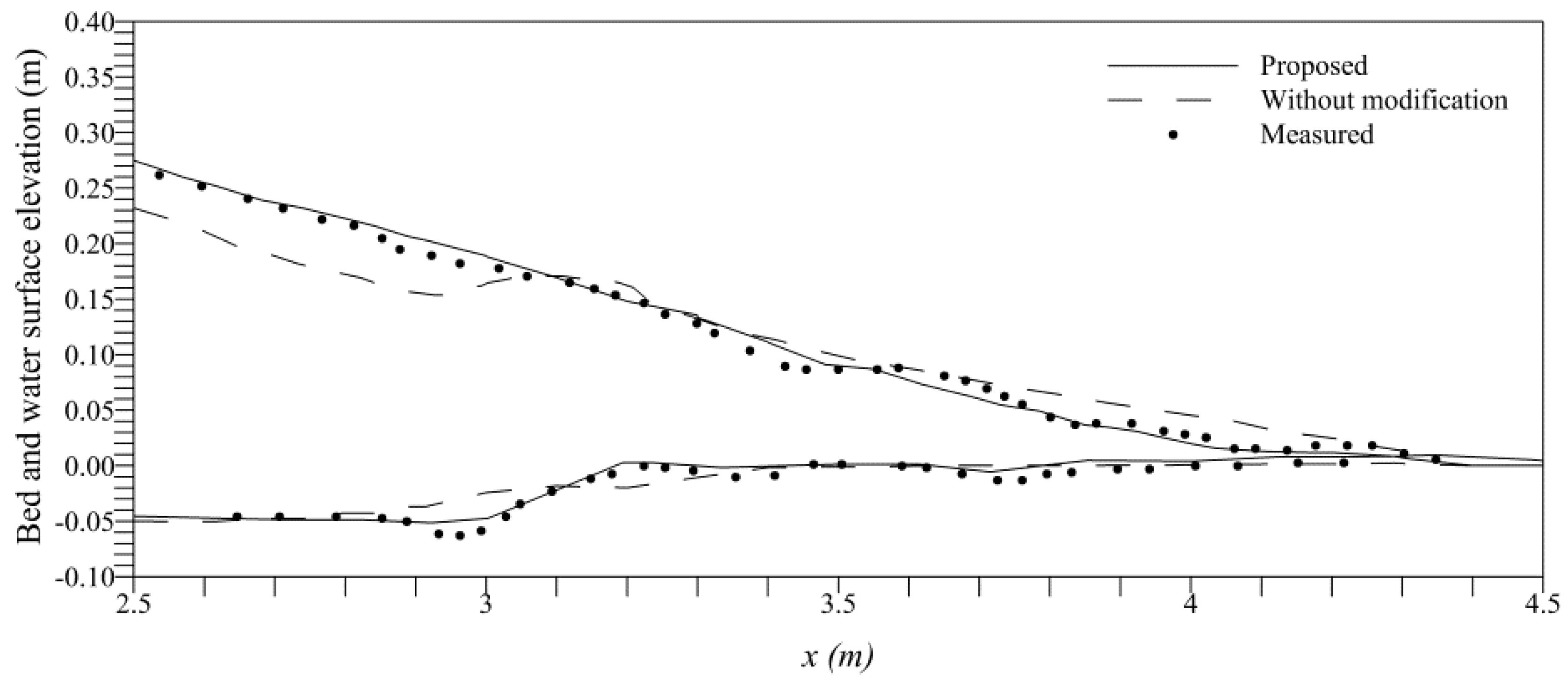
Figure 6 shows the comparison of water surface and bed profiles for configuration 2 at t = 0.5 s. Although the bed profile is in fair agreement with experimental results, the wave-front in the present study slightly leads the measured. The leading wave-front may be due to the excessive erosion of the bed step, which, according to Evangelista et al. (2013), occurs due to a greater angle of internal friction than a vertical slope of the bed step. The angle of internal friction is not considered in the Grass formula, which may be the reason for the slightly lower bed scour estimates and the leading wave fronts.
Results for configuration 3 at t = 0.25 s, 0.75 s and 1.25 s after dam-break are presented in Figure 7. In Figure 7a, the numerical studies under-predict the bed scour; this is due to the sudden removal of the gate in experiments, which causes excessive soil collapse at the start of dam-break. However, at later instants, when the bed layer smoothens, the results of the proposed scheme are in good agreement with the experimental results as compared to the scheme without modification, as shown in Figure 7b,c. The differences in position of wave fronts likely occur for the same reason discussed for configuration 1.
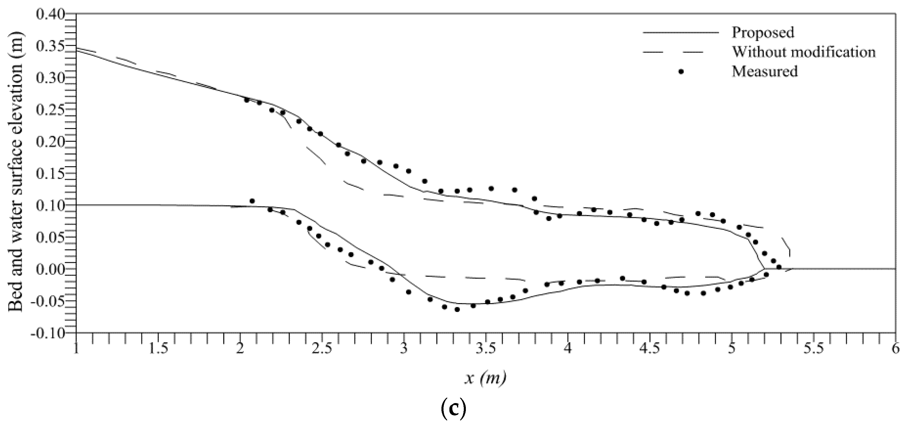
Figure 8 shows the results for configuration 4 after t = 0.25 s, 0.50 s and 1.0 s after dam-break. The formation of the hydraulic jump is observed at x = 3.2 m and x = 3.6 m at t = 0.25 s and t = 0.50 s, respectively, and occurs when the flow is in transition from super critical to sub critical. However, the jump vanishes at t = 1.0 s and the wave front becomes flatter due to the inertia of the water downstream of the dam. Following the previous trend, the proposed scheme gives better predictions for bed evolution and wave-front propagation for this case also. Overall comparisons in Figure 5, Figure 6, Figure 7 and Figure 8 show reasonably good agreement with experimental measurements. These results demonstrate the proposed scheme’s ability to accurately predict bed evolution and wave-front transition under dam-break flows, with efficient handling of shocks.
4.5. Sensitivity Analysis
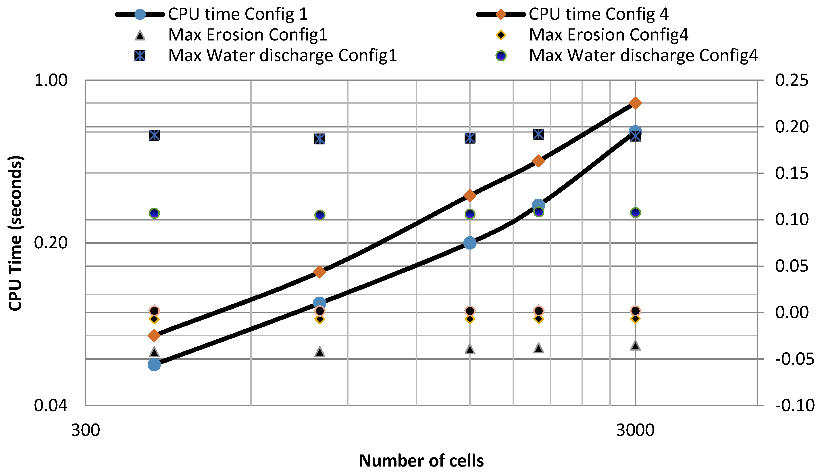
A sensitivity analysis is performed to study the effects of mesh resolution on computational time, flow variables (discharge), and bed elevation. The model is simulated for five consecutively refined mesh systems; the number of elements from the coarsest to finest mesh is 400, 1000, 2000, 3500, and 5000. The analysis was performed on an Intel® Core TM i7-3770 (8 M Cache, 3.4 GHz) computer with 8 GB DDR3 RAM. Figure 9 shows the increase in simulation time with mesh refinement for configurations 1 and 4. It can be observed in Figure 9 that there are no significant changes in water depth and velocity with mesh refinement. This shows that the proposed scheme satisfies the primary requirement of robust solvers to be computationally efficient and independent of the mesh resolution.
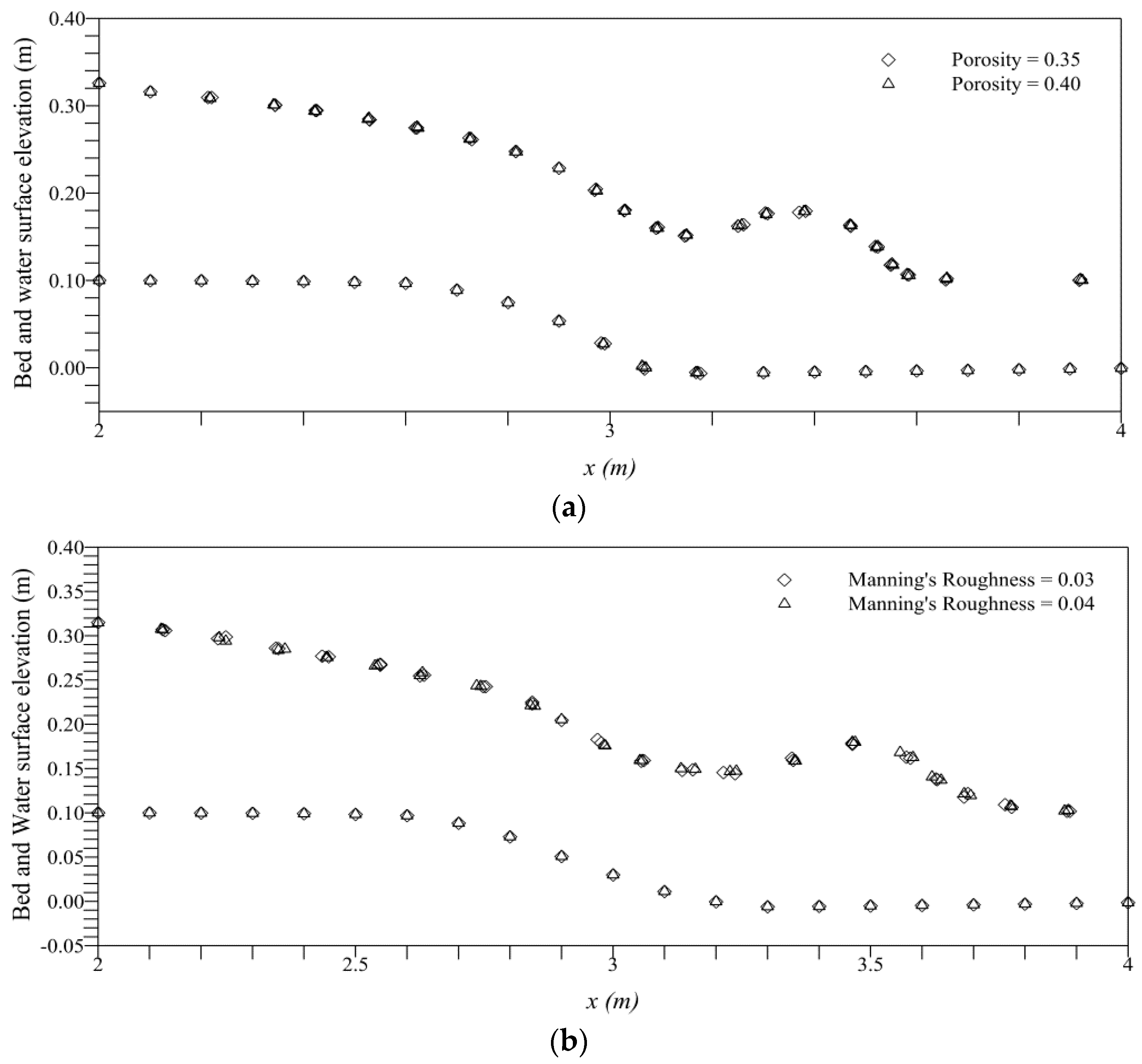
Sensitivity of the sediment parameters, including Manning’s roughness (n) and porosity (p) are also analyzed for the laboratory scale test discussed in Section 4.4. We consider configurations 1 and 4 for comparison purposes. Figure 10 shows the variation in results as each parameter varies with the rest kept constant. In Figure 10a,b, no significant changes are observed in bed erosion with changes in sediment parameters, which again can be attributed to the presence of downstream water. Figure 10b shows that with changes in bed roughness, the hydraulic jump extends beyond the measured value (shown in Figure 8b), which is due to the lagging wave front causing a delay in the formation of the jump.
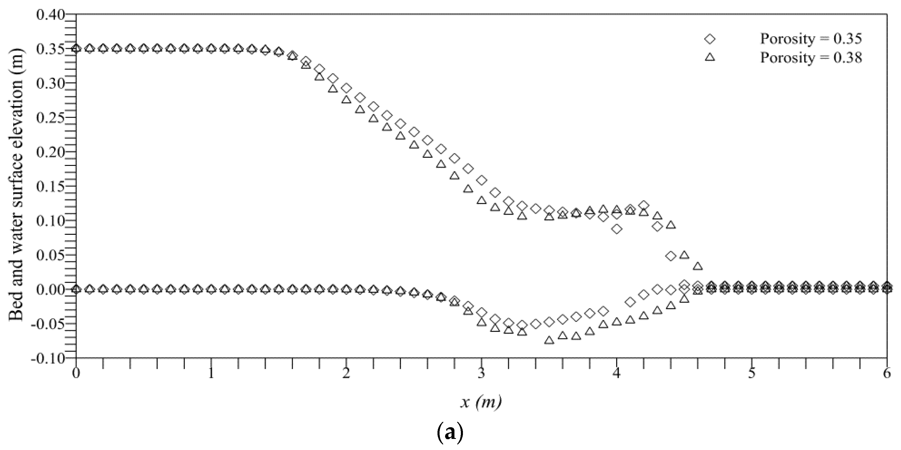
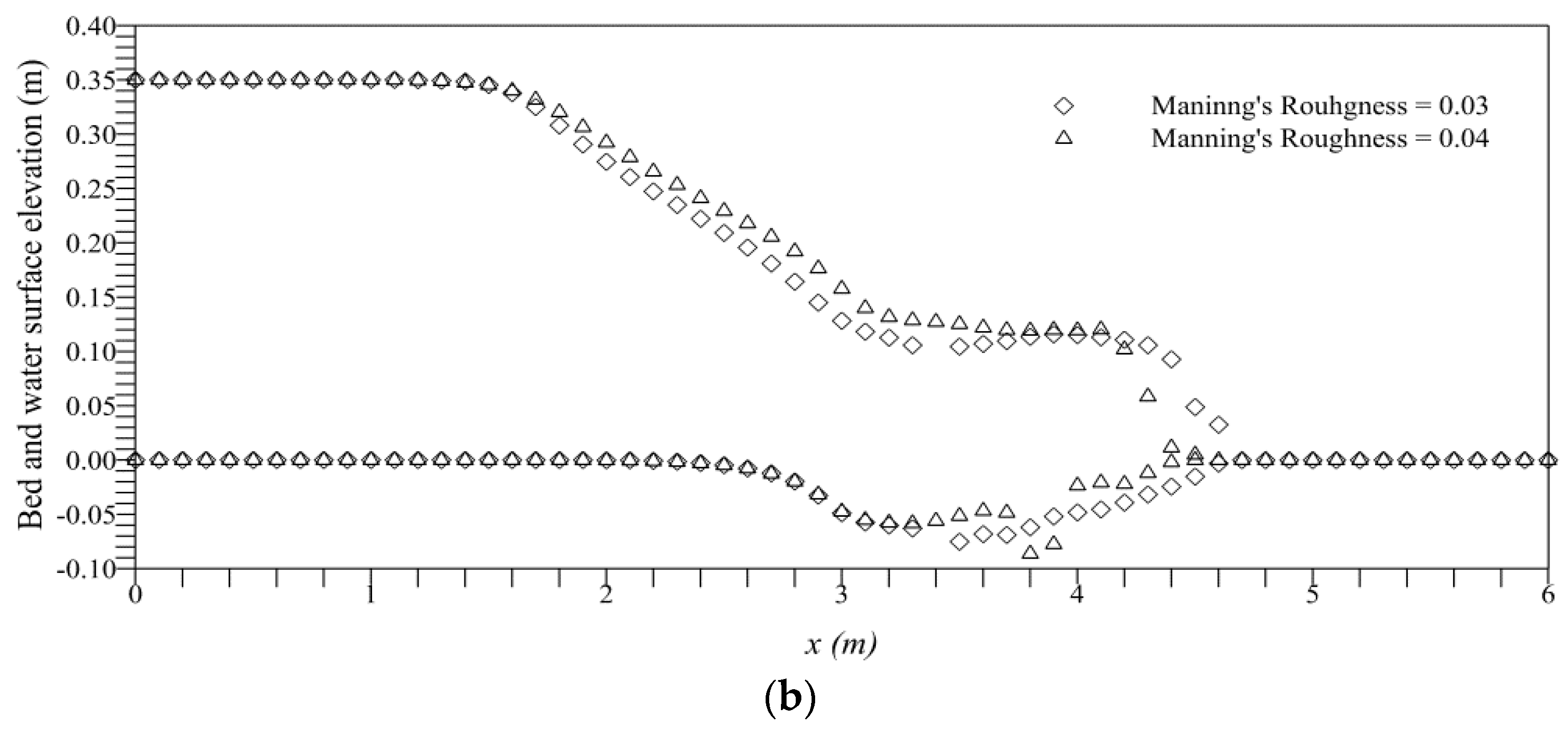
For configuration 1, the variation in porosity (0.35–0.38) and Manning’s roughness (0.03–0.04) show significant increases in bed erosion, as seen in Figure 11a,b, respectively. The increase in values of both parameters result from increased interaction of sediment and water related to direct contact of water particles with sediment, due to absence of tail-water. This scenario also results in a higher resistance offered to the flow in comparison to configuration 4. We conclude that the absence of tail-water makes the erodible bed more sensitive to changes in sediment parameters, and can significantly affect the bed evolution under wave-front propagation, as observed in Figure 11.
5. Conclusions
This paper introduces a simple and robust model for bed evolution and its effects on water surface profile under rapidly varying flows using a formulation comprised of coupled Saint-Venant and Exner equations. A finite volume method of Godunov type is adopted to obtain solutions for the coupled system. The proposed method for the calculation of variables in the star region has proven to give better results than the previous numerical studies, and is able to reproduce the experimental results very satisfactorily. The sensitivity analysis shows that the proposed scheme is computationally very efficient, which is important for schemes modeling sediment flow since the wave structure involved is usually complicated. It was observed for all cases that the values of bed friction, porosity, and dimensional constant (A), which represents the intensity of interaction between water and sediment particles, significantly influence the stability and accuracy of the model, and the position of the hydraulic jump. Analytical solutions, original experimental data, and numerical results are adopted for comparisons. The accuracy of the model is tested for a number of cases, highlighting its efficiency and adaptability under various conditions.
Acknowledgments
This research was supported by the National Research Foundation of Korea (NRF) grant funded by the Korea Government (MSIP) (No. 2015R1A2A1A15054097).
Author Contributions
Khawar Rehman designed and performed the simulations, analyzed the data, and wrote the paper; Yong-sik Cho contributed providing materials/analysis tools and ideas in developing the manuscript.
Conflicts of Interest
The authors declare no conflict of interest.
References
- Carrivick, J.L.; Manville, V.; Graettinger, A.; Cronin, S.J. Coupled fluid dynamics-sediment transport modelling of a Crater Lake break-out lahar: Mt. Ruapehu, New Zealand. J. Hydrol. 2010, 388, 399–413. [Google Scholar] [CrossRef]
- Kim, J.; Ivanov, V.Y.; Katopodes, N.D. Modeling erosion and sedimentation coupled with hydrological and overland flow processes at the watershed scale. Water Resour. Res. 2013, 49, 5134–5154. [Google Scholar] [CrossRef]
- Guan, M.; Wright, N.G.; Sleigh, P.A.; Carrivick, L.J. Assessment of hydro-morphodynamic modelling and geomorphological impacts of a sediment-charged jökulhlaup, at Sólheimajökull, Iceland. J. Hydrol. 2015, 530, 336–349. [Google Scholar] [CrossRef]
- Huang, W.; Cao, Z.; Carling, P.; Pender, G. Coupled 2D hydrodynamic and sediment transport modeling of megaflood due to glacier dam-break in Altai Mountains, Southern Siberia. J. Mt. Sci. 2014, 11, 1442–1453. [Google Scholar] [CrossRef]
- Benkhaldoun, F.; Sahmim, S.; Seaïd, M. A two-dimensional finite volume morphodynamic model on unstructured triangular grids. Int. J. Numer. Methods Fluids 2010, 63, 1296–1327. [Google Scholar] [CrossRef]
- Hudson, J.; Damgaard, J.; Dodd, N.; Chesher, T.; Cooper, A. Numerical approaches for 1D morphodynamic modelling. Coast. Eng. 2005, 52, 691–707. [Google Scholar] [CrossRef]
- Liang, Q. A coupled morphodynamic model for applications involving wetting and drying. J. Hydrodyn. Ser. B 2011, 23, 273–281. [Google Scholar] [CrossRef]
- Wu, W.; Wang, S.S. One-dimensional modeling of dam-break flow over movable beds. J. Hydraul. Eng. ASCE 2007, 133, 48–58. [Google Scholar] [CrossRef]
- Cao, Z.; Pender, G.; Wallis, S.; Carling, P. Computational dam-break hydraulics over erodible sediment bed. J. Hydraul. Eng. ASCE 2004, 130, 689–703. [Google Scholar] [CrossRef]
- Xia, J.; Lin, B.; Falconer, R.A.; Wang, G. Modelling dam-break flows over mobile beds using a 2D coupled approach. Adv. Water Resour. 2010, 33, 171–183. [Google Scholar] [CrossRef]
- Campisano, A.; Creaco, E.; Modica, C. Experimental and numerical analysis of the scouring effects of flushing waves on sediment deposits. J. Hydrol. 2004, 299, 324–334. [Google Scholar] [CrossRef]
- Hudson, J. Numerical Techniques for Morphodynamic Modelling. Ph.D. Thesis, University of Reading, Reading, UK, October 2001. [Google Scholar]
- Goutière, L.; Soares-Frazão, S.; Savary, C.; Laraichi, T.; Zech, Y. One-dimensional model for transient flows involving bed-load sediment transport and changes in flow regimes. J. Hydraul. Eng. ASCE 2008, 134, 726–735. [Google Scholar] [CrossRef]
- Soares-Frazão, S.; Zech, Y. HLLC scheme with novel wave speed estimators appropriate for two dimensional shallow water flow on erodible bed. Int. J. Numer. Methods Fluids 2011, 66, 1019–1036. [Google Scholar] [CrossRef]
- Grass, A.J. Sediment Transport by Waves and Currents; University College London, Department of Civil Engineering: London, UK, 1981. [Google Scholar]
- Meyer-Peter, E.; Müller, R. Formulas for bed-load transport. In Proceedings of the 2nd Meeting of the International Association for Hydraulic Structures Research, Stockholm, Sweden, 7 June 1948.
- Van Rijn, L.C. Sediment transport, part I: Bed load transport. J. Hydraul. Eng. ASCE 1984, 110, 1431–1456. [Google Scholar] [CrossRef]
- Van Rijn, L.C. Sediment transport, Part II: Suspended load transport. J. Hydraul. Eng. ASCE 1984, 110, 1613–1641. [Google Scholar] [CrossRef]
- Van Rijn, L.C. Sediment transport, part III: Bed forms and alluvial roughness. J. Hydraul. Eng. ASCE 1984, 110, 1733–1754. [Google Scholar] [CrossRef]
- Nielsen, P. Coastal Bottom Boundary Layers and Sediment Transport; World Scientific: Tuck Link, Singapore, 1992; Volume 4. [Google Scholar]
- El Kadi Abderrezzak, K.; Paquier, A. Applicability of sediment transport capacity formulas to dam-break flows over movable beds. J. Hydraul. Eng. ASCE 2010, 137, 209–221. [Google Scholar] [CrossRef]
- Murillo, J.; García-Navarro, P. An Exner-based coupled model for two-dimensional transient flow over erodible bed. J. Comput. Phys. 2010, 229, 8704–8732. [Google Scholar] [CrossRef]
- Liu, X.; Landry, B.; García, M. Two-dimensional scour simulations based on coupled model of shallow water equations and sediment transport on unstructured meshes. Coast. Eng. 2008, 55, 800–810. [Google Scholar] [CrossRef]
- Murillo, J.; García-Navarro, P. Improved Riemann solvers for complex transport in two-dimensional unsteady shallow flow. J. Comput. Phys. 2011, 230, 7202–7239. [Google Scholar] [CrossRef]
- Hudson, J.; Sweby, P.K. Formulations for numerically approximating hyperbolic systems governing sediment transport. J. Sci. Comput. 2003, 19, 225–252. [Google Scholar] [CrossRef]
- Hudson, J.; Sweby, P.K. A high-resolution scheme for the equations governing 2D bed-load sediment transport. Int. J. Numer. Methods Fluids 2005, 47, 1085–1091. [Google Scholar] [CrossRef]
- Castro Díaz, M.J.; Fernández-Nieto, E.D.; Ferreiro, A.; Parés, C. Two-dimensional sediment transport models in shallow water equations. A second order finite volume approach on unstructured meshes. Comput. Methods Appl. Mech. Eng. 2009, 198, 2520–2538. [Google Scholar] [CrossRef]
- Toro, E.F. Riemann problems and the WAF method for solving the two-dimensional shallow water equations. Philos. Trans. R. Soc. Lond. Ser. A Phys. Eng. Sci. 1992, 338, 43–68. [Google Scholar] [CrossRef]
- Batten, P.; Clarke, N.; Lambert, C.; Causon, D. On the choice of wavespeeds for the HLLC Riemann solver. SIAM J. Sci. Comput. 1997, 18, 1553–1570. [Google Scholar] [CrossRef]
- Roe, P. Approximate Riemann solvers, parameter vectors, and difference schemes. J. Comput. Phys. 1997, 135, 250–258. [Google Scholar] [CrossRef]
- Mottura, L.; Vigevano, L.; Zaccanti, M. An evaluation of Roe’s scheme generalizations for equilibrium real gas flows. J. Comput. Phys. 1997, 138, 354–399. [Google Scholar] [CrossRef]
- Glaister, P. An approximate linearised Riemann solver for the Euler equations for real gases. J. Comput. Phys. 1988, 74, 382–408. [Google Scholar] [CrossRef]
- Hu, X.; Adams, N.; Iaccarino, G. On the HLLC Riemann solver for interface interaction in compressible multi-fluid flow. J. Comput. Phys. 2009, 228, 6572–6589. [Google Scholar] [CrossRef]
- Toro, E. Shock-Capturing Methods for Free-Surface Shallow Flows; Wiley: Chichester, UK, 2001. [Google Scholar]
- Holmes, D.; Connell, S.; Engines, G.A. Solution of the 2D Navier-Stokes Equations on Unstructured Adaptive Grids; American Institute of Aeronautics and Astronautics: Reston, VA, USA, 1989. [Google Scholar]
- Delis, A.; Skeels, C.; Ryrie, S. Evaluation of some approximate Riemann solvers for transient open channel flows. J. Hydraul. Res. 2000, 38, 217–231. [Google Scholar] [CrossRef]
- Kim, D.-H.; Cho, Y.-S.; Kim, H.-J. Well-Balanced Scheme between Flux and Source Terms for Computation of Shallow-Water Equations over Irregular Bathymetry. J. Eng. Mech. 2008, 134, 277–290. [Google Scholar] [CrossRef]
- Li, S.; Duffy, C.J. Fully coupled approach to modeling shallow water flow, sediment transport, and bed evolution in rivers. Water Resour. Res. 2011, 47. [Google Scholar] [CrossRef]
- Stoker, J.J. Water Waves: The Mathematical Theory with Applications; John Wiley & Sons: Hoboken, NJ, USA, 2011; Volume 36. [Google Scholar]
- Bellal, M. Fluvial Morphodynamics in Super and Transcritical Flows: Experimental and Analytical Approaches. Ph.D. Thesis, University College London, London, UK, August 2012. [Google Scholar]
- Briganti, R.; Dodd, N.; Kelly, D.; Pokrajac, D. An efficient and flexible solver for the simulation of the morphodynamics of fast evolving flows on coarse sediment beaches. Int. J. Numer. Methods Fluids 2012, 69, 859–877. [Google Scholar] [CrossRef]
- Kelly, D.M.; Dodd, N. Floating grid characteristics method for unsteady flow over a mobile bed. Comput. Fluids 2009, 38, 899–909. [Google Scholar] [CrossRef]
- Spinewine, B.; Zech, Y. Small-scale laboratory dam-break waves on movable beds. J. Hydraul. Res. 2007, 45, 73–86. [Google Scholar] [CrossRef]
- Evangelista, S.; Altinakar, M.S.; Di Cristo, C.; Leopardi, A. Simulation of dam-break waves on movable beds using a multi-stage centered scheme. Int. J. Sediment Res. 2013, 28, 269–284. [Google Scholar] [CrossRef]
- Guan, M.; Wright, N.G.; Andrew Sleigh, P. Multimode morphodynamic model for sediment-laden flows and geomorphic impacts. J. Hydraul. Eng. ASCE 2015, 141. [Google Scholar] [CrossRef]
Figure 1.
Comparison of water levels for dam-break over rigid bed for: (a) wet bed; and (b) dry bed.
Figure 1.
Comparison of water levels for dam-break over rigid bed for: (a) wet bed; and (b) dry bed.


Figure 2.
Bed aggradation from sediment overloading.
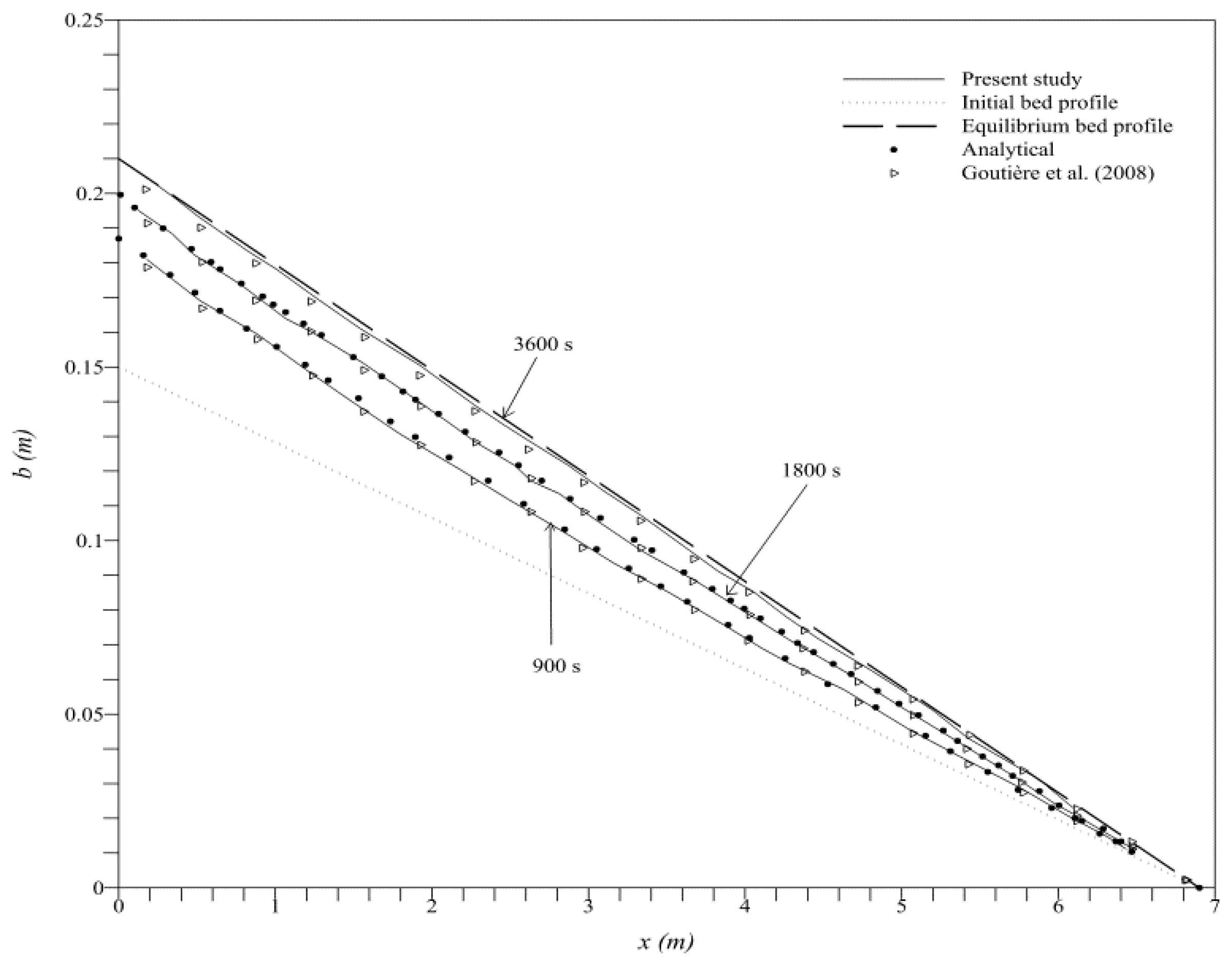
Figure 3.
Comparison of (a) water level; (b) bed deformation; and (c) velocity with exact solution for dam-break over an erodible bed.
Figure 3.
Comparison of (a) water level; (b) bed deformation; and (c) velocity with exact solution for dam-break over an erodible bed.

Figure 4.
Initial Configurations for dam-break over sand bed: (a) Configuration 1; (b) Configuration 2; (c) Configuration 3; and (d) Configuration 4.
Figure 4.
Initial Configurations for dam-break over sand bed: (a) Configuration 1; (b) Configuration 2; (c) Configuration 3; and (d) Configuration 4.

Figure 5.
Numerical and experimental results of dam-break for configuration 1: (a) t = 0.25 s; (b) t = 0.75 s; and (c) t = 1.25 s.
Figure 5.
Numerical and experimental results of dam-break for configuration 1: (a) t = 0.25 s; (b) t = 0.75 s; and (c) t = 1.25 s.

Figure 6.
Numerical and experimental results of dam-break for configuration 2 at t = 0.5 s.

Figure 7.
Numerical and experimental results of dam-break for Configuration 3: (a) t = 0.25 s; (b) t = 0.75 s; and (c) t = 1.25 s.
Figure 7.
Numerical and experimental results of dam-break for Configuration 3: (a) t = 0.25 s; (b) t = 0.75 s; and (c) t = 1.25 s.
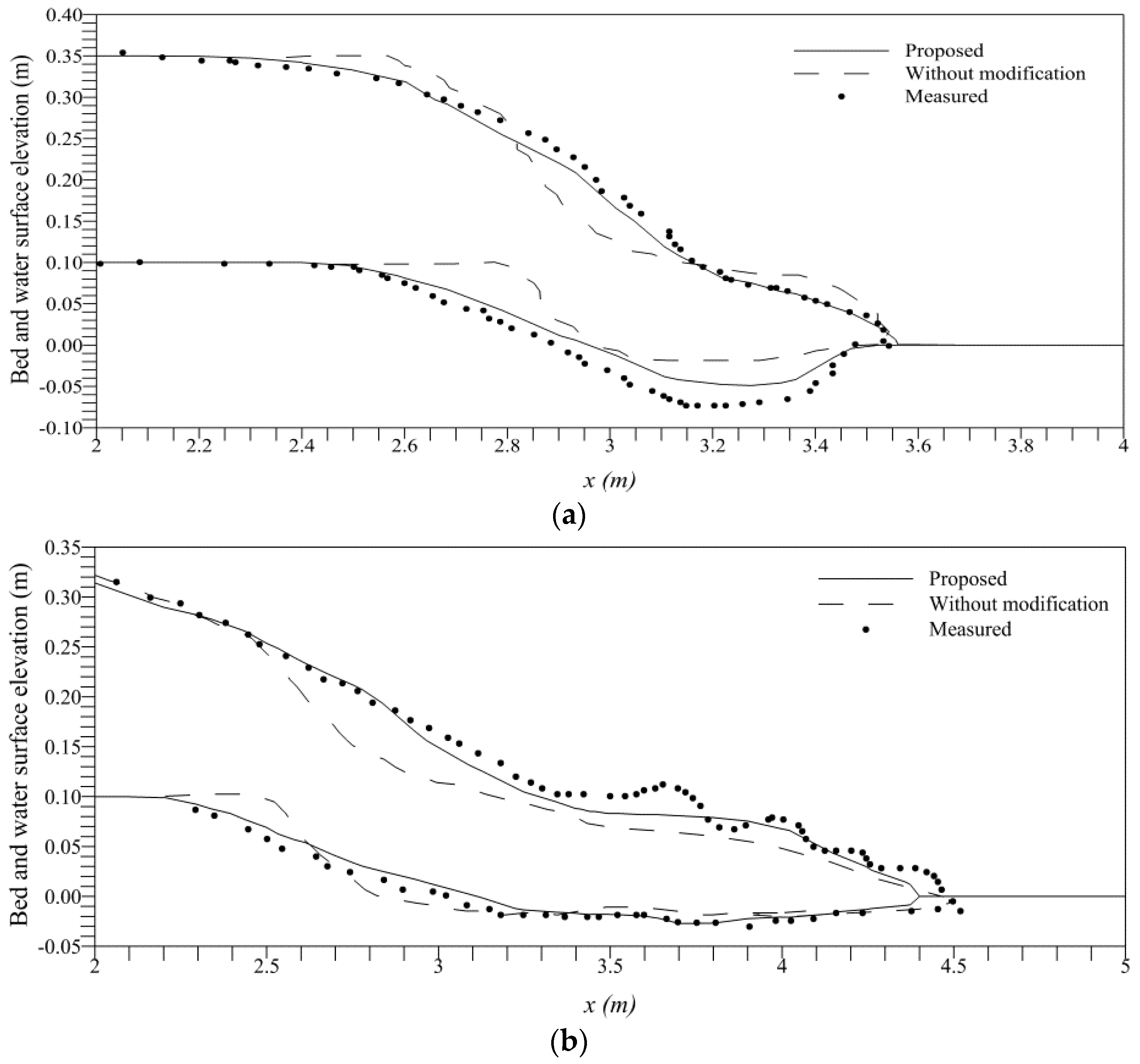

Figure 8.
Numerical and experimental results of dam-break for Configuration 4: (a) t = 0.25 s; (b) t = 0.5 s; and (c) t = 1.0 s.
Figure 8.
Numerical and experimental results of dam-break for Configuration 4: (a) t = 0.25 s; (b) t = 0.5 s; and (c) t = 1.0 s.
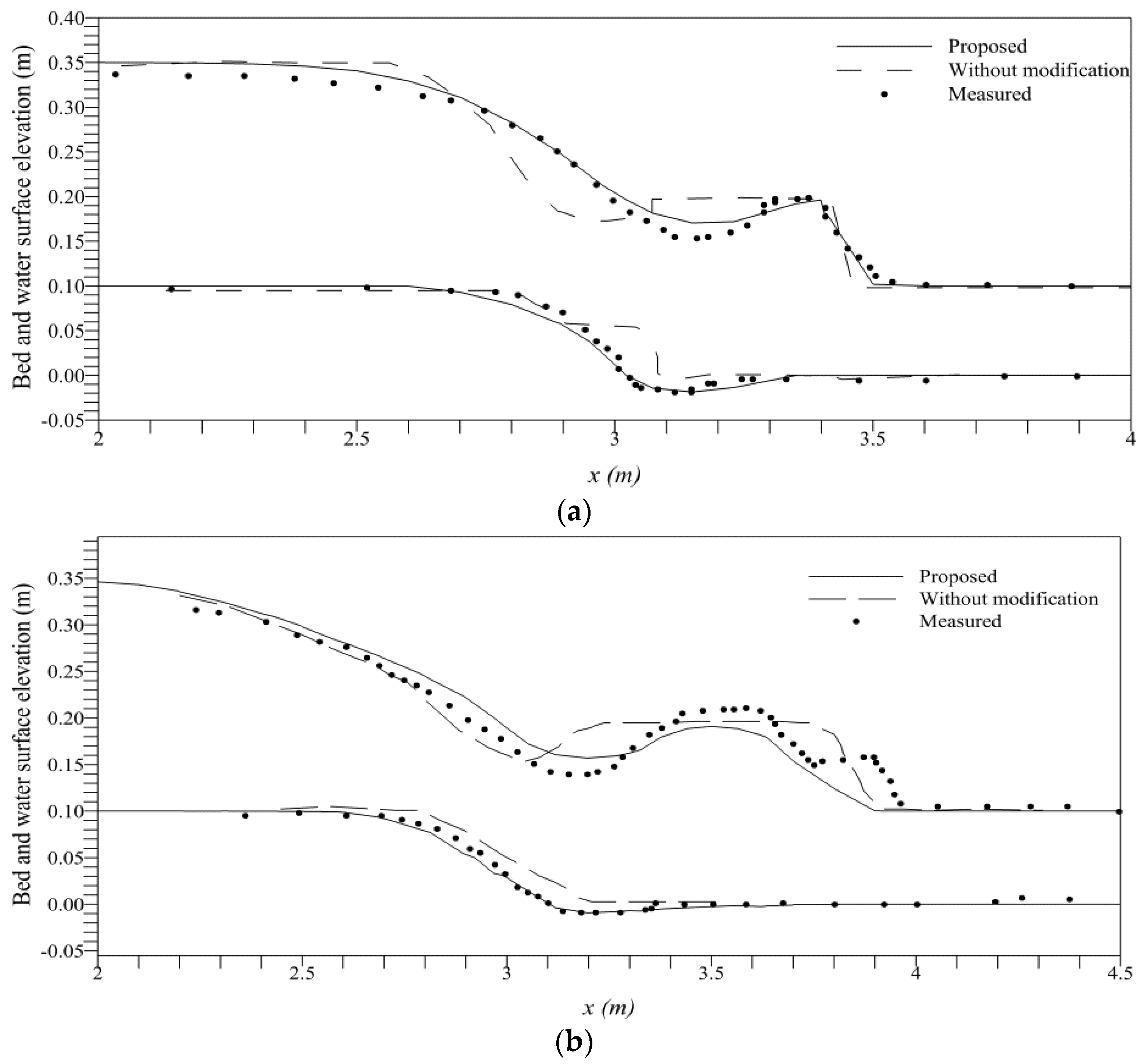
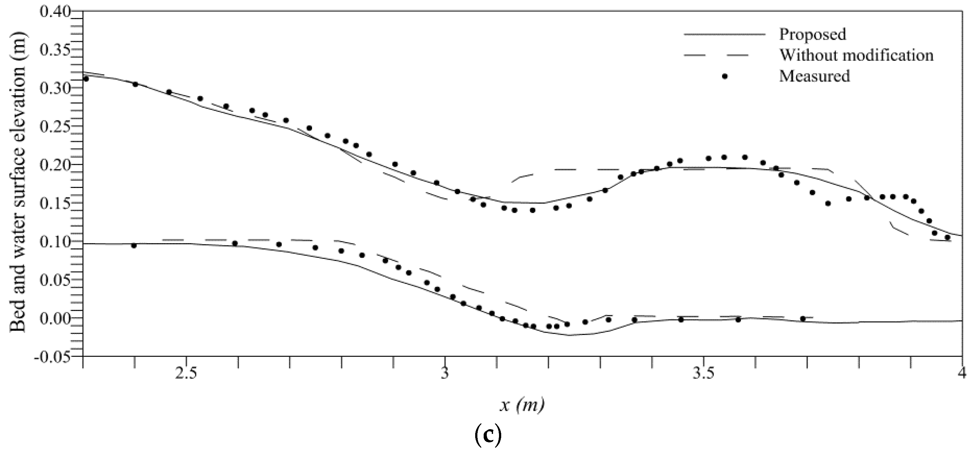
Figure 9.
CPU-time performance and Sensitivity of hydraulic and morphologic parameters to mesh refinement.
Figure 9.
CPU-time performance and Sensitivity of hydraulic and morphologic parameters to mesh refinement.

Figure 10.
Sensitivity analysis for Configuration 4 to model parameters at t = 0.75 s: (a) porosity p; and (b) Manning’s roughness n.
Figure 10.
Sensitivity analysis for Configuration 4 to model parameters at t = 0.75 s: (a) porosity p; and (b) Manning’s roughness n.

Figure 11.
Sensitivity analysis for Configuration 1 to the model parameters at t = 0.75 s: (a) porosity p; and (b) Manning’s n.
Figure 11.
Sensitivity analysis for Configuration 1 to the model parameters at t = 0.75 s: (a) porosity p; and (b) Manning’s n.


© 2016 by the authors; licensee MDPI, Basel, Switzerland. This article is an open access article distributed under the terms and conditions of the Creative Commons Attribution (CC-BY) license (http://creativecommons.org/licenses/by/4.0/).
Share and Cite
MDPI and ACS Style
Rehman, K.; Cho, Y.-S. Bed Evolution under Rapidly Varying Flows by a New Method for Wave Speed Estimation. Water 2016, 8, 212. https://doi.org/10.3390/w8050212
AMA Style
Rehman K, Cho Y-S. Bed Evolution under Rapidly Varying Flows by a New Method for Wave Speed Estimation. Water. 2016; 8(5):212. https://doi.org/10.3390/w8050212
Chicago/Turabian StyleRehman, Khawar, and Yong-Sik Cho. 2016. "Bed Evolution under Rapidly Varying Flows by a New Method for Wave Speed Estimation" Water 8, no. 5: 212. https://doi.org/10.3390/w8050212
Note that from the first issue of 2016, this journal uses article numbers instead of page numbers. See further details here.