Using High-Resolution Data to Test Parameter Sensitivity of the Distributed Hydrological Model HydroGeoSphere

Abstract

Parameterization of physically based and distributed hydrological models for mesoscale catchments remains challenging because the commonly available data base is insufficient for calibration. In this paper, we parameterize a mesoscale catchment for the distributed model HydroGeoSphere by transferring evapotranspiration parameters calibrated at a highly-equipped headwater catchment in addition to literature data. Based on this parameterization, the sensitivity of the mesoscale catchment to spatial variability in land use, potential evapotranspiration and precipitation and of the headwater catchment to mesoscale soil and land use data was conducted. Simulations of the mesoscale catchment with transferred parameters reproduced daily discharge dynamics and monthly evapotranspiration of grassland, deciduous and coniferous vegetation in a satisfactory manner. Precipitation was the most sensitive input data with respect to total runoff and peak flow rates, while simulated evapotranspiration components and patterns were most sensitive to spatially distributed land use parameterization. At the headwater catchment, coarse soil data resulted in a change in runoff generating processes based on the interplay between higher wetness prior to a rainfall event, enhanced groundwater level rise and accordingly, lower transpiration rates. Our results indicate that the direct transfer of parameters is a promising method to benefit highly equipped simulations of the headwater catchments.

1. Introduction

The usage of integrated and distributed hydrological models (e.g., HydroGeoSphere [1], ParFlow-CLM [2], MIKE-SHE [3] and Cathy [4]) has considerably increased during the last decade alongside advances in computer and measurement technology. It is widely acknowledged that hydrological models integrating the surface and subsurface flow systems have on the one hand, a great potential to give insights into temporal and spatial patterns of fluxes, state variables and feedback [5,6,7,8,9]. On the other hand, the complexity of these models causes overparameterization (e.g., [10]) and hinders transferability of achieved simulation as well as parameterization results to other spatio-temporal scales (e.g., [11,12]).

Distributed observation networks, necessary for a reliable calibration and validation of spatial patterns simulated by 3D-models—for example soil moisture sensor networks—are typically only available for small test sites [13], such as the Wüstebach catchment in Germany [14] or the Little Washita catchment in the United States [2]. Due to their high data demand, distributed hydrological 3D-models are currently predominantly used for small-scale applications [6,8,15]. Rare examples at large scales include the study of Goderniaux et al. [16] who estimated climate change effects on groundwater reserves in a 480 km² mesoscale catchment with HydroGeoSphere and the study of Rahman et al. [17] who applied ParFlow-CLM to a 2364 km² macroscale catchment to investigate spatio-temporal patterns of land surface mass and energy fluxes.

The rarity of simulations at meso- (>10 km²) or macroscale (>1000 km²) catchments is in sharp contrast to potential feedback with boundary processes at these scales. For example, Hauck et al. [18] stated that the simulation of convection could be improved with more detailed information on spatial and vertical distribution of soil moisture.

Modeling catchments larger than headwater catchments is closely connected to a decrease in quantity and quality of available calibration data, especially concerning their spatial distribution. In addition, mesoscale catchments can exhibit stronger variability in land use and climate variables. Thus, assembling a data base which is sufficient for a reliable calibration of distributed and process-based models is a challenging task. Given the large uncertainties inherent in mesoscale catchment modeling with distributed hydrological models, it is necessary to facilitate the model setup and to investigate the sensitivity of model parameters and input data. The model setup can be facilitated by using prior knowledge of parameters and their spatial distribution. For example, parameters can be regionalized with different methods from other catchments or parameters can be directly transferred from subcatchments, as described in Bogena and Diekkrüger [19]. According to Moriasi et al. [20], a sensitivity analysis investigates the reaction of the model output to changes in parameters or input data and is a requirement for a successful calibration. A sensitivity analysis of a highly heterogeneous mesoscale catchment must include the investigation of spatial heterogeneity in climate input data and of model parameters. Similar to the transfer of parameters, information about the sensitivity of model parameters can potentially be inferred from a subcatchment, if the spatial and temporal discretization does not change.

In this study we use the distributed hydrological 3D-model HydroGeoSphere in a nested simulation approach to conduct a sensitivity analysis across scales. The first research aspect investigates the sensitivity of discharge, water balance and evapotranspiration patterns to spatial heterogeneity in land use, potential evapotranspiration and precipitation at the mesoscale. Evapotranspiration parameters for the mesoscale catchment setup are taken from existing research and are directly transferred from calibrated and validated simulations of a well-equipped sub-catchment. As these transferred evapotranspiration parameters originate from a homogeneously covered spruce forest, the question arises if they can be applied for evapotranspiration simulation of different land use types. Thus, the second research aspect gives a validation of simulated monthly evapotranspiration for the different land use types of the mesoscale catchment. Apart from transferred parameters, the setup of the mesoscale catchment involves the incorporation of land use data and soil parameters that are different to the subcatchment due to change in resolution and heterogeneity. Thus, the third research aspect of this study is a sensitivity analysis of the subcatchment to land use and soil parameters used for the setup of the mesoscale catchment.

The simulation results at the mesoscale catchment, in terms of discharge dynamics and monthly evapotranspiration, highlight the potential of heavily instrumented test sites to deliver reliable estimates of evapotranspiration parameters for the simulation of different land use conditions.

2. Materials and Methods

2.1. Description of the Study Area

The Erkensruhr catchment is located in western Germany close to the Belgian border (Figure 1A). It is 41.9 km² large and its elevation increases from 286 m.a.s.l. to 631 m.a.s.l. in eastern and southern directions. The slope varies between 0° and 7° in flatter areas in the central and south-eastern catchment part. It rapidly increases with proximity to the river bed with slopes above 25° in the northern catchment part. Mean annual temperatures range between 7.6 °C at high and 10 °C at low altitudes. The catchment is characterized by a strong west-east gradient in precipitation with a mean annual precipitation of 1150 mm over areas west to the catchment and 740 mm over areas east to the catchment.

Cambisols are the dominant soil type in the Erkensruhr catchment, whereas river valleys are dominated by Gleysols and Planosols (Figure 1). Silt loam is the dominant soil texture in the first soil layer (mean depth: 0.8 m) and clay in the second layer (mean depth: 1.8 m). In the second layer, Cambisols, Gleysols and Vertisols exhibit an high skeleton content of at least 66% with a maximum skeleton content of 90%, whereas Planosols have a mean skeleton content of only 10%. Native rocks are Devonian clayshales with sandstone intrusions and filled fractures [21].

The Erkensruhr catchment is dominated by coniferous forest (mainly Picea abies) in the southern part; and deciduous forest (mainly Fagus sylvatica) in the north-western part. Grassland and pasture predominantly occur in the eastern and central parts of the catchment (Figure 1). Arable land and urban areas cover only less than 3% of the catchment area.

The Wüstebach headwater catchment is located at the southern border of the Erkensruhr catchment. It is 0.385 km² large [22] with a mean annual precipitation of 1220 mm (1979–1999 [23]) and has been completely covered with Norwegian spruce (Picea Abies [24]) since 1950. The catchment is heavily monitored due to hydrological fluxes and states, as well as transportation of matter [25].

2.2. Model Description

In our study we applied the fully coupled surface-subsurface flow model HydroGeoSphere (HGS; [1,16,26]) in the parallel mode [27]. HGS solves the 3D Richards equation for subsurface flow and the 2D wave approximations of the Saint Venant equation for surface flow. The simulation of interception and evapotranspiration follows the approach of Kristensen and Jensen [28]. Interception is modeled with a bucket approach, where precipitation reaches the ground when the precipitation rate exceeds the maximum interception storage and its evaporation. Interception storage is emptied prior to other evapotranspiration processes.

The transpiration rate depends (1) on LAI according to a linear correlation function; (2) on a root distribution function which distributes root extraction among the root zone confined by the maximum root depth; (3) on the difference between potential and canopy evapotranspiration and (4) nonlinearly on the current soil moisture (see [26] for a detailed description).

The impact of the LAI on transpiration depends on two fitting parameters. With the chosen LAI and fitting parameters for the Wüstebach catchment, the function is compatible.

The maximum root depth and the root extraction function are sensitive parameters in term of soil moisture simulation. Quadratic and cubic root distribution functions are used in the context of this study.

Transpiration nonlinearly depends on soil moisture according to the following rules: the transpiration is zero for soil moistures (θ) below the wilting point (θ_wp) and beyond the anoxic limit (θ_an). Between the wilting point (θ_wp) and the field capacity (θ_fc), as between the oxic (θ_o) and anoxic limits (θ_an), the transpiration increases to the potential rate depending on a dimensionless fitting parameter. Between the field capacity (θ_fc) and the oxic limit (θ_o), the actual transpiration occurs at the potential rate. The oxic (θ_o) and anoxic limits (θ_an) were the most sensitive parameters in the Wüstebach study in terms of simulated transpiration amount [15].

To distinguish between different runoff components, the hydraulic mixing cell method was applied to HGS [29]. This method extracts discharge components from flux and storage information of the model for rectangular cells. Currently, the method distinguishes between (1) baseflow to the stream and to overland areas (return flow) and (2) direct rainfall input into the stream and onto overland areas. As the baseflow filter does currently not support gridded input data, it was only applied for the simulations of the Wüstebach headwater catchment.

In this study, the dual node approach for the implementation of the surface domain was used. This means that the 2D surface flow domain follows the uppermost node layer of the subsurface domain. Flow equations of both domains are coupled via an interconnection term describing leakage through an artificial skin layer on top of the uppermost 3D subsurface nodes. The subsurface domain was discretized using 3D-prisms.

2.3. Conceptual Model

In order to capture the variation in catchment slope (refer to Chapter 2.1), the Erkensruhr mesh consisted of two zones with different grid spacing. The riparian zone contained those catchment parts that either have a slope of more than 15° or are in a maximum distance of 200 m to the river. The riparian zone and the slope of the hill zone were discretized using 100 m and 200 m spacing, respectively. The Wüstebach catchment was fully discretized using 100 m spacing to facilitate the comparison with the independent Wüstebach simulation of Cornelissen et al. [15] who used the same spacing. The subsurface domain was 2 meters deep and was resolved in 28 numerical layers with increasing thickness in increasing distance to the infiltration zone.

Simulations of the Erkensruhr and the Wüstebach catchment started with a spin-up period of half a year. Initial conditions were set equal to the results of a 20 year warm-up run for the Wüstebach and a 10 year warm-up run for the Erkensruhr. At the catchment outlet, the critical depth boundary condition was assigned while all other boundaries were no flow boundaries.

2.4. Data Base

Table 1. Data sources, availability, spatial and temporal resolution and measurement location of input data used in the Wüstebach and Erkensruhr simulations.

Data Type	Source	Spatial Resolution	Temporal Resolution	Availability	Measurement Location
Wüstebach and Erkensruhr simulations
Digital Elevation	Land Surveying Office of North Rhine-Westphalia	10 × 10 m2	-	-	-
Climate	TERENO Observation Network	1 Station	Hourly	Since 2009	Schöneseiffen (3.4 km east to Wüstebach)
Wüstebach simulations
Soil	Geological Survey of North Rhine-Westphalia	1:2500	-	-	-
Precipitation	German Weather Service	1 Station	Hourly	Since 2001	Kalterherberg (9.6 km west to Wüstebach)
Erkensruhr simulations
Soil	Geological Survey of North Rhine-Westphalia	1:50,000	-	-	-
Precipitation (Radar Data)	Wasserverband Eifel-Rur	1 × 1 km2	5 min	Since 2002	-
Land Use	[34]	15 × 15 m2	-	Since 2008	-

summarizes spatial and temporal input data used in both simulations and data only used in either the Wüstebach or the Erkensruhr simulations.

The term mesoscale is used in the context of this study to refer to catchments with a size larger than 10 km² and to distinguish the low resolution data set of the Erkensruhr catchment (e.g., soil data at 1:50,000) from the high resolution data set of the headwater catchment Wüstebach (e.g., soil data at 1:2500).

For the calculation of potential evapotranspiration (PET hereafter), the climate station at Schöneseiffen (at 610 m.a.s.l.; refer to Figure 1 for its location) was used for all simulations of both catchments. Due to the high correlation between altitude and temperature (R²: 0.95) with a mean temperature gradient of 0.695 °C/100 m calculated with measured data from 5 stations near the catchment, it was necessary to account for a spatial variability in PET in the Erkensruhr catchment. The climate data of the reference climate station Schöneseiffen were arbitrarily defined to be valid for the 50 m above and below the station height, leading to the definition of the following altitude layers: ≤360, 360–460, 460–560, >560 m.a.s.l. To compute the FAO-Penman-Monteith PET [30], a new weighted albedo value according to the fraction of land use was defined for each altitude layer. The albedo values were taken from Breuer et al. [31]. This method resulted in an increase in PET (between the lowest and the highest altitude class) of 113 mm in 2010 and 126 mm in 2011. The total amount of PET did not change compared to the homogeneous PET because 80% of the catchment has an altitude above 460 m.

Precipitation data for simulations with homogeneous precipitation were taken from the station of Kalterherberg (9.6 km west of the catchment; refer to Figure 1 for its location) and corrected according to the method of Richter [32]. The simulation of the Erkensruhr catchment with distributed precipitation used ground-truth corrected precipitation radar data with a spatial resolution of 1 × 1 km² and a temporal resolution of 5 min provided by the local water-authority (Wasserverband Eifel-Rur). A snow model following the degree-day method [33] was applied to both precipitation data sets at hourly time steps and subsequently aggregated to daily time steps.

2.5. Parameterization and Calibration

In HGS the nonlinear relationship between soil suction and soil moisture is described by the van-Genuchten-Mualem (VGM) model [35]. The VGM parameters were derived from soil texture and bulk density using the pedotransfer function of Rawls and Brakensiek [36] and if applicable, the function of Brakensiek and Rawls [37] to account for skeleton content. We assumed a litter layer of 5 cm thickness using VGM parameters as suggested by Bogena et al. [38] at both catchments. In the context of this study, the litter layer is defined as the layer overlaying the actual soil horizons with a mixture of differently decomposed foliage. In the case of the Erkensruhr catchment, saturated conductivity values were directly taken from the soil map. At the Wüstebach, they were calculated with the pedotransfer function of Brakensiek et al. 1986 [39] including the influence of rock fragments on conductivity. At the Erkensruhr, the soil map does not show any skeleton content in the first layer. These differences in methodology resulted in large deviations in conductivity values (refer to Tables S1 and S2). For the simulations of the Wüstebach catchment (independently of the Erkensruhr), the VGM parameters were calculated for a model resolution of 25 m. To investigate the effects of spatial aggregation of soil parameter [15,40], mean VGM parameters were calculated for the 100 m setups used in this study. Parameters used for these setups are given in Tables S1 and S2 as area averaged mean values for the 5 soil types of the Erkensruhr catchment.

Mean monthly LAI values for agriculture, grassland and deciduous broadleaf forests were computed as an arithmetic mean of the 8-day LAI values between 2003 and 2013 from the Moderate Resolution Imaging Spectroradiometer (MODIS) with a spatial resolution of 1 km².

Meinen et al. [41] and Dannowski and Wurbs [42] report the distribution of root biomass with soil depth for Fagus sylvatica and the extensive grassland. HGS offers 4 different root distribution functions: constant, linear, quadratic and cubic decay. A quadratic decay function was fitted (R²: 0.99) to the data for deciduous forest and a cubic decay function was fitted (R²: 0.90) to the data for extensive grassland.

A calibration to discharge measurements of the Erkensruhr catchment was not performed in this study because calibration of a distributed model to an aggregated value (in this case discharge) leads to equifinality in the model parameters [43]. In addition, the process-based model HGS does not contain any empirical values related to discharge calculation. Instead, calibrated evapotranspiration parameters from the Wüstebach were used. The oxic and anoxic transpiration limits of HGS which influence the dependency between transpiration rate and soil moisture have been calibrated in Cornelissen et al. [15] to match soil moisture dynamics and an actual evapotranspiration of 40% of catchment rainfall. Soil moisture [44] and actual evapotranspiration [14] was measured at the coniferous forest of the Wüstebach catchment. As measured actual evapotranspiration data from a nearby grassland site (Marius Schmidt, personal communication) suggest an actual evapotranspiration of 60% of local precipitation rates, the oxic and anoxic transpiration limits for grassland areas were set to a value which allows transpiration to be unlimited, if the saturation exceeds the field capacity.

Table 2. Land use parameters used in the Erkensruhr simulation study.

	Land Use Class	Coniferous	Deciduous	Grassland	Agriculture	Urban
Parameter
Fraction of land use type (%)		40	19	38	2	1
Mean annual LAI (-)		6.7 1	1.93 2	1.51 2	1.16 2	25.5 2
Evaporation depth (m)		0.2 1	Transferred
Root depth (m)		0.5 1	1.8 3	0.35 4	1.0 5	Deactivation
Root and evaporation distribution function (-)		Quadratic 1	Quadratic 6	Cubic 4	Quadratic 5	Deactivation
Transpiration fitting parameters (-)		0.3 1,0.2 1, 1.0 1	Transferred			Deactivation
Transpiration limiting saturations (Wilting point, Field capacity, Oxic, Anoxic) (-)		0.3 1, 0.4 1, 0.89 7, 0.97 7	Transferred	0.3 1, 0.4 1, 1.0, 1.0	Transferred
Canopy storage (mm)		0.8	0.83 8	1.0 8	2.5 8	15.0 5
Evaporation limiting saturations (min, max) (-)		0.3 1, 0.4 1	Transferred

¹: [40]; ²: MODIS data; ³: [31] (Fagus Sylvatica on deep loam in Germany); ⁴: Values for extensive grassland by Dannowski and Wurbs [42]; ⁵: Assumption; ⁶: [41]; ⁷: [15]; ⁸: Mean interception capacities for grassland (1.5 mm), agriculture (2.9 mm) and Fagus sylvatica (1.6 mm) according to Breuer et al. [31] and Mendel [45] were divided by corresponding mean LAI (1.51 for grassland, 1.16 for agriculture and 1.93 for Fagus sylvatica) according to MODIS data.

lists all vegetation parameters used in the simulation together with their sources. The term “transferred” used in the table means that the parameter was equal to the calibrated parameters for coniferous forest of the Wüstebach catchment.

2.6. Modeling Procedure

In this study we compare ten model scenarios with different parameterizations: six scenarios of the Wüstebach headwater catchment and four scenarios of the Erkensruhr catchment with unique combinations of soil and land use parameters (refer to

Table 3. Summary of abbreviations of conducted simulations with applied soil and land use data.

Simulation Scenarios	Soil Data	Land Use	Additional Information
Wüstebach Catchment
Wbach	Wüstebach	Coniferous	Reference scenario
WbachDeci	Wüstebach	Deciduous
WbachGrass	Wüstebach	Grassland
WbachEsoilConi	Erkensruhr	Coniferous
WbachEsoilDeci	Erkensruhr	Deciduous
WbachEsoilGrass	Erkensruhr	Grassland
Erkensruhr Catchment
Erk	Erkensruhr	Coniferous
Erk_LN	Erkensruhr	All	Distributed land use
Erk_LN_PET	Erkensruhr	All	Distributed land use and potential evapotranspiration
Erk_LN_PET_P	Erkensruhr	All	Distributed land use, potential evapotranspiration and precipitation

for an overview).

For the first set of model setups, the coniferous forest of the Wüstebach reference setup (Wbach) was changed to deciduous forest (WbachDeci) and grassland (WbachGrass) while keeping all other inputs constant. For the second set of model setups, the mesoscale soil parameters of the Erkensruhr were applied to the Wüstebach simulation using the three different land use parameterizations for coniferous (WbachEsoilConi), deciduous (WbachEsoilDeci) and grassland (WbachEsoilGrass).

For the base setup of the Erkensruhr catchment (Erk) we used distributed soil data but assumed homogeneous land use, PET and precipitation. Land use, PET and precipitation were set equal to the Wüstebach catchment. Spatial heterogeneity of land use, PET and precipitation (in the form of radar data) was introduced step-wise into the Erkensruhr setup leading to three additional simulations: Erk_LN, Erk_LN_PET and Erk_LN_PET_P. This procedure means that the simulation Erk_LN still uses PET and precipitation equal to that of the Wüstebach catchment, but soil and land use data originated from the Erkensruhr catchment. In the Erk_LN_PET simulation, only precipitation is equal to the Wüstebach. In the Erk_LN_PET_P simulation, all inputs originate from the Erkensruhr. Additionally, a simulation run using spatially mean radar data was accomplished to separate possible effects of the precipitation pattern from the effects of changes in precipitation amount (results not shown).

The reference model setup for the Wüstebach simulations corresponds to calibrated and validated 100 m setup without bedrock inclusion used in Cornelissen et al. [15]. Please note that differences between model results reported in Cornelissen et al. [15] and those reported in this study resulted from the usage of a new version of HGS that corrected a bug in the interception module and differences in residual saturation and porosities. In Cornelissen et al. [15] residual saturations and porosities were calibrated to measured soil moistures. The calibration resulted in an increase in residual saturations and porosities approximately equal to the correction for skeleton content according to Brakensiek and Rawls [37]. Due to the fact that no skeleton content was reported in the first layer in the Erkensruhr soil data, we ran the simulations Wbach, WbachDeci and WbachGrass (refer to Table 3) with uncalibrated residual saturations and porosities. We acknowledge that the usage of different residual saturations and porosities slightly changed the impact of transpiration parameters on actual evapotranspiration and soil moisture simulation.

2.7. Measures of Model Performance

We applied three statistical measures to quantify the quality of discharge simulations (also refer to Equations (1) and (2)): (1) the bias, defined as the ratio between simulated and observed mean discharge of a given time period; (2) the coefficient of variation measuring the agreement between observed and simulated distributions of discharge values; (3) the R² (squared form of Pearson’s correlation coefficient) as an indicator of linear correlation. All values were calculated separately for the hydrological summer and winter periods due to substantial performance differences. As all measures reached their optimum value at unity, numerals larger or smaller than 1.0 given in Figures 3 and 8 can be interpreted as percentage deviations from the optimum.

$$Bias=\frac{\mu \left(Q_{sim}\right)}{\mu \left(Q_{mes}\right)}$$

(1)

$$Coefficient of Variation= \frac{\frac{\sigma \left(Q_{sim}\right)}{\mu \left(Q_{sim}\right)}}{\frac{\sigma \left(Q_{mes}\right)}{\mu \left(Q_{mes}\right)}}$$

(2)

with $\mu \left(Q_{sim}\right)$ and $\mu \left(Q_{mes}\right)$ being simulated and observed mean discharge and $\sigma \left(Q_{sim}\right)$ and $\sigma \left(Q_{mes}\right)$ being simulated and observed standard deviation. Following Moriasi et al. [20], we rate values of all three measures larger than 0.9 and smaller than 1.1 as “very good”, values between 0.9 (1.1) and 0.85 (1.15) as “good”, values between 0.85 (1.15) and 0.75 (1.25) as “satisfactory” and all other values as unsatisfactory.

3. Results

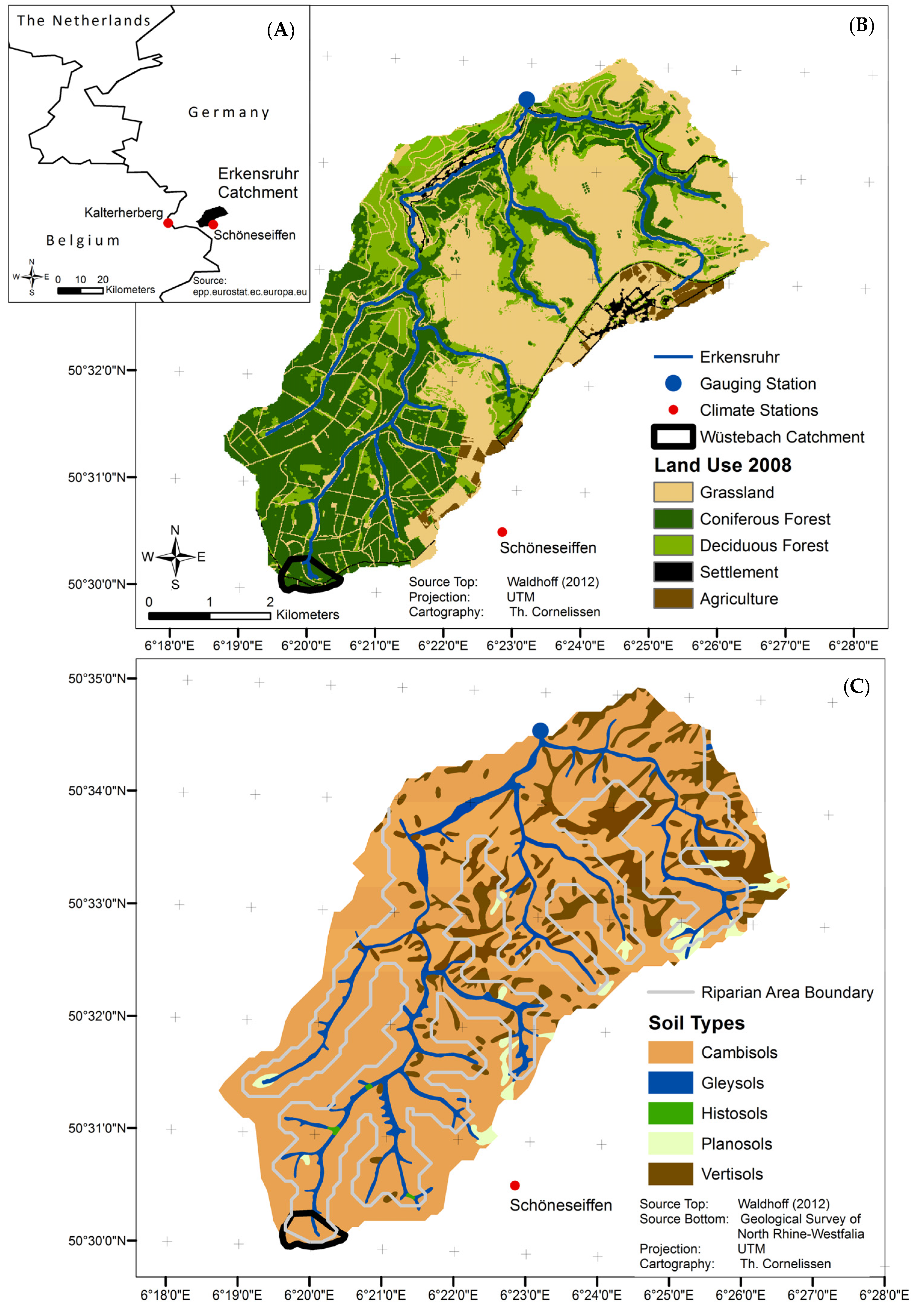
3.1. Influence of Mesoscale Soil and Land Use Parameterization on the Simulation of the Headwater Catchment

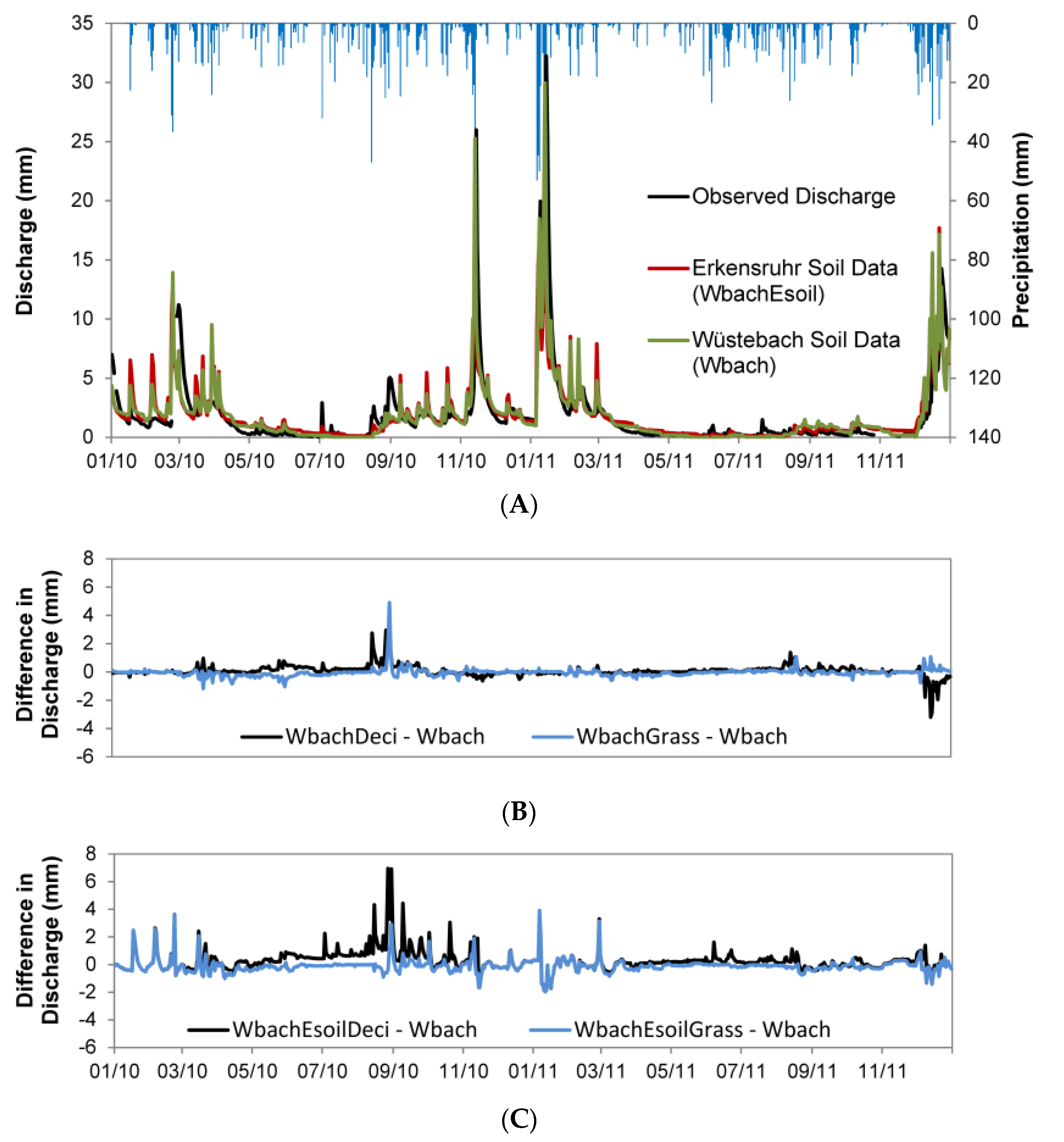
Figure 2A shows measured and simulated discharge rates for the two simulations Wbach and WbachEsoilConi for the years 2010 and 2011. Observed discharge was characterized by a strong seasonality with a pronounced low flow period during the summer and high variability during snow dominated periods in the winter. Generally, both simulation scenarios reproduced the discharge dynamics well but overestimated peaks during the winter (due to an overestimation of snow melt by the snow model) and omitted some peaks during the summer. The usage of mesoscale soil data from the Erkensruhr (model scenario WbachEsoilConi) intensified the tendency to overestimate peak discharge rates.

Differences in discharge between the reference simulation Wbach and the simulations WbachDeci and WbachGrass (Figure 2B) were smaller than ±0.5 mm for more than 90% of the simulation period indicating a weak sensitivity of discharge to changes in land use parameterization. Higher discharge rates of WbachDeci and WbachGrass in late summer 2010 resulted from differences in LAI development and corresponding changes in interception. At the end of 2011, differences in discharge resulted from differences in soil moisture. The WbachDeci simulation had lower soil moistures in all depths than the Wbach simulation and therefore rainfall was primarily replenishing the water storage. The WbachGrass simulation had highest soil moisture at the same time and accordingly, highest discharge rates. In Figure 2C, differences between Wbach and the WbachEsoilDeci and WbachEsoilGrass simulations are shown. Both simulations produced higher discharge rates during both years with an extreme overestimation during 2010 of the WbachEsoilDeci model scenario.

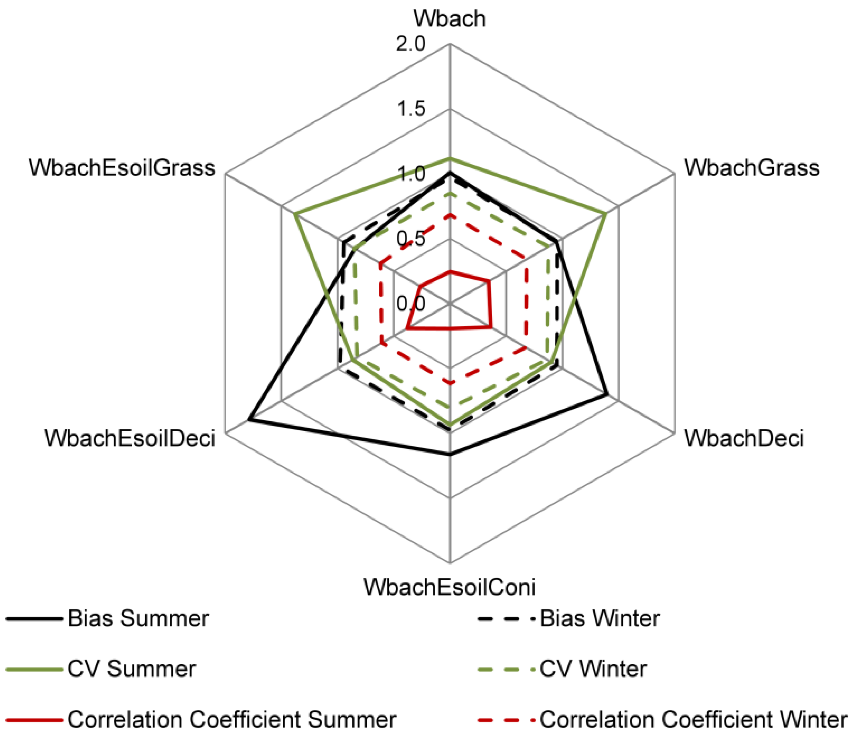
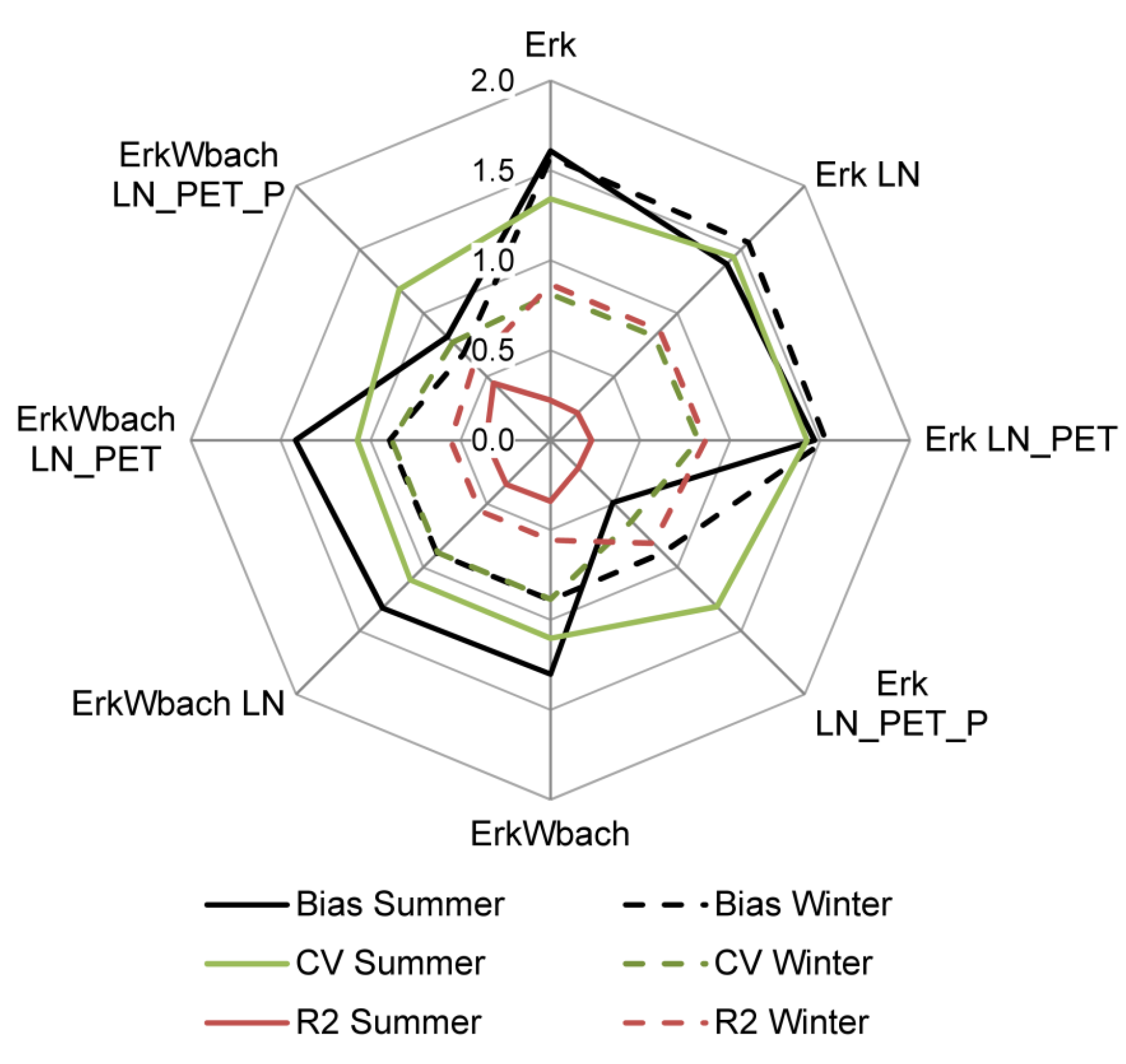
Figure 3 summarizes statistical measures of model performance for the hydrological winter 2010/2011 and—as a mean value—for the hydrological summer periods in 2010 and 2011.

All statistical measures varied more strongly between simulations during summer than during winter because (1) differences in evapotranspiration simulation only became apparent during summer and (2) small changes in discharge amount and timing had a high impact on statistical measures during the low flow period.

During winter, all model scenarios produced unsatisfactory R² values (0.61–0.68) but very good bias values (0.94–0.98); the coefficient of variation was lower than unity for all simulations due to the underestimation of discharge variability during winter.

Changing land use primarily affected the coefficient of variation during the hydrological summer with increases for grassland and decreases for deciduous forest. In contrast, a change in soil data heavily influenced the bias and the R². The unique behavior of the simulation WbachEsoilDeci in terms of very high increases in bias and R² compared to WbachDeci has already been mentioned in the previous paragraph. The reason for this increase in bias will be further analyzed in this chapter and in the discussion section.

The water balance of the Wüstebach simulations (

Table 4. Water balance components for Wüstebach simulations.

	Simulation	2010
Water Balance Setup Component		Wbach	Wbach Deci	WbachGrass	Wbach Esoil Coni	Wbach Esoil Deci	Wbach Esoil Grass
Rainfall (mm)		1226
Potential ET (mm)		694
Measured Discharge (mm)		608
Transpiration (mm)		232	227	279	195	99	282
Evaporation (mm)		247	254	289	247	256	293
Actual Evapotranspiration (mm)		479	481	568	442	355	575
Discharge 1 (mm)		611	657	591	647	764	587
Baseflow (%)		76	76	75	64	62	63
Infiltration (mm)		968	992	1011	891	879	954
		2011
Rainfall (mm)		1348
Potential ET (mm)		756
Measured Discharge (mm)		630
Transpiration (mm)		272	312	290	247	250	306
Evaporation (mm)		273	283	314	273	289	325
Actual Evapotranspiration (mm)		545	595	604	520	539	631
Discharge 1 (mm)		637	640	626	652	673	594
Baseflow (%)		62	64	60	56	58	53
Infiltration (mm)		894	959	960	832	870	896

¹: Yearly sums of simulated discharge exclude time steps with gaps in measured discharge data.

) showed some interesting features concerning evapotranspiration components and infiltration sums. The total amount of actual evapotranspiration significantly changed between different land uses with highest values for WbachGrass due to the changes in transpiration parameters. In 2010, the amount of actual evapotranspiration for the WbachDeci simulation equaled that of Wbach but in 2011 the evapotranspiration was higher by 50 mm. Infiltration sums and fractions of subsurface flow varied between the years but not between simulation variants using the same soil data.

Comparing simulations with high-resolution soil data of the Wüstebach to those with mesoscale Erkensruhr soil data, significant differences in the water balance components and in the fractions of subsurface flow became apparent. For both forested land uses, actual evapotranspiration decreased by 37 mm (2010) and 25 mm (2011) for coniferous and by 126 mm (2010) and 56 mm (2011) for the deciduous forest. The decrease in evapotranspiration resulted from a decrease in infiltration sums by 77 mm (2010) and 62 mm (2011) for coniferous and by 113 mm (2010) and 89 mm (2011) for the deciduous forest. Despite the decrease in infiltration sums, discharge sums were much higher and as a result, the fraction of subsurface flow decreased by 12%–14% in 2010 and 6%–7% in 2011. The effect described above was stronger in 2010 than in 2011. In April and May 2010 precipitation rates were larger than PET rates but in April and May 2011 precipitation rates were lower. The surplus in PET significantly reduced soil moisture in 2011 thus dampening the effect of mesoscale soil data on runoff generation processes.

In contrast to the forest land uses, the WbachEsoilGrass scenario showed small changes in total evapotranspiration (≤27 mm) and correspondingly lowest variations in infiltration sums. The deviations in the water balance during 2010 and 2011 arose from intense rainfall rates during December in both years.

Comparing water balance results of the setups Wbach and WbachEsoilConi to measured water balance components mentioned in Cornelissen et al. [15], the following observations can be stated: (1) Simulated discharge amounts match well with measured discharge rates for the Wbach scenario in both years; the WbachEsoilConi overestimated discharge by 20 mm (2010) and 40 mm (2011); (2) The estimated fraction of evaporation (20% of precipitation) matches very well to simulated fractions; (3) The amounts of actual evapotranspiration are largely underestimated in 2011 by 50 mm (Wbach) and 80 mm (WbachEsoilConi) due to low transpiration rates.

In the context of this paper, soil moisture simulation results are compared between simulations but not to measurements. For a detailed comparison between simulated and measured soil moisture of the Wüstebach catchment, the reader is referred to Cornelissen et al. (2014) [15].

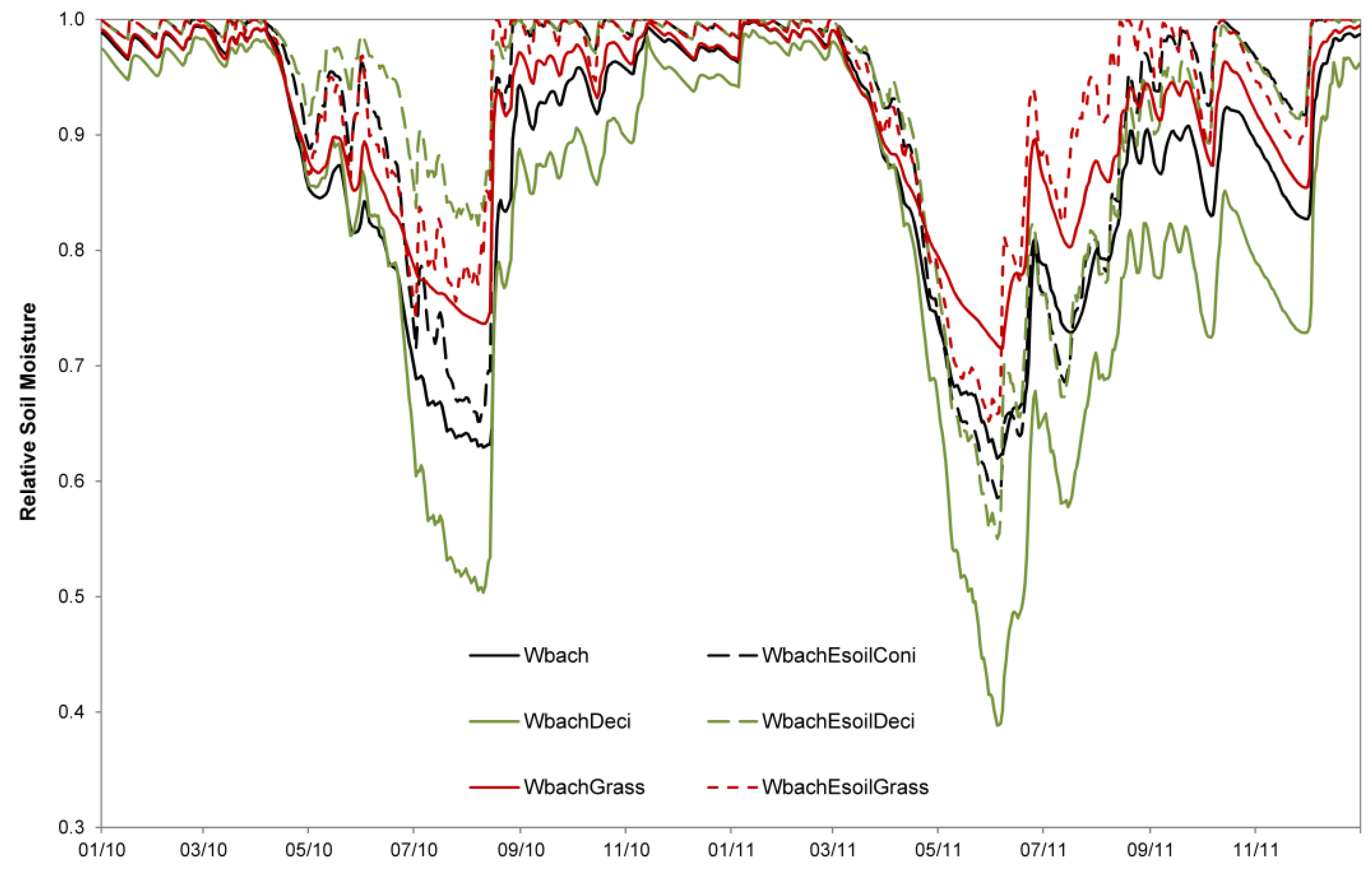
We noted pronounced differences in simulated soil moisture dynamics between land use types at all depths. At 5 cm depth, differences were most pronounced during August and July 2010 when the WbachDeci simulation maintained soil moisture values above 0.5 while soil moisture for both the Wbach and the WbachGrass simulations dropped below 0.3. In August and July 2011, the WbachDeci simulation was again the wettest but differences to Wbach and WbachGrass were smaller. The Wbach and WbachGrass scenarios showed small differences at 5 cm depth because their root depth (refer to Table 2) was comparably small with 0.5 m and 0.35 m respectively. At 20 cm depth (Figure 4) the WbachDeci scenario produced the lowest soil moisture in both years. During July and August of both years, WbachGrass and Wbach maintained soil moisture values of about 0.6 while WbachDeci dropped below 0.4 in 2011. In both years, the WbachGrass scenario produced the highest soil moisture. At 50 cm depth a clear hierarchy following root depths was found in both years with the highest moistures for WbachGrass (featuring the lowest root depth) and lowest values for WbachDeci (featuring the highest root depth).

The usage of mesoscale soil data generally increased soil wetness and intensified short term soil moisture dynamics down to 50 cm depth. Differences were again most pronounced for the simulation with deciduous land use. The increased soil moisture dynamic with coarser soil data led to a decrease in infiltration and transpiration with a corresponding increase in discharge.

The relationship between mean soil moisture and its standard deviation (σ_θ(<θ>)) showed little variations between different land use types at 5 cm depth (Figure 5). Simulations with Erkensruhr soil data produced a steeper slope with higher standard deviations at the same moisture. This is attributed to the fact that the VGM parameters of the model setups used in this study were aggregated from a model resolution of 25 m ([15]; also refer to Chapter 2.5). As demonstrated recently by Qu et al. [46] the shape of σ_θ(<θ>) can be explained to a large extent by the spatial variance of soil hydraulic properties.

3.2. Influence of Parameter Regionalization and Spatially Distributed Input Data on the Simulation of the Mesoscale Catchment

In the following, the results of the four Erkensruhr simulations are analyzed separately for the whole Erkensruhr catchment and for the Wüstebach sub-catchment. Water balance results were only available for the Erkensruhr as HGS does not enable the export of water balance results for sub-catchments.

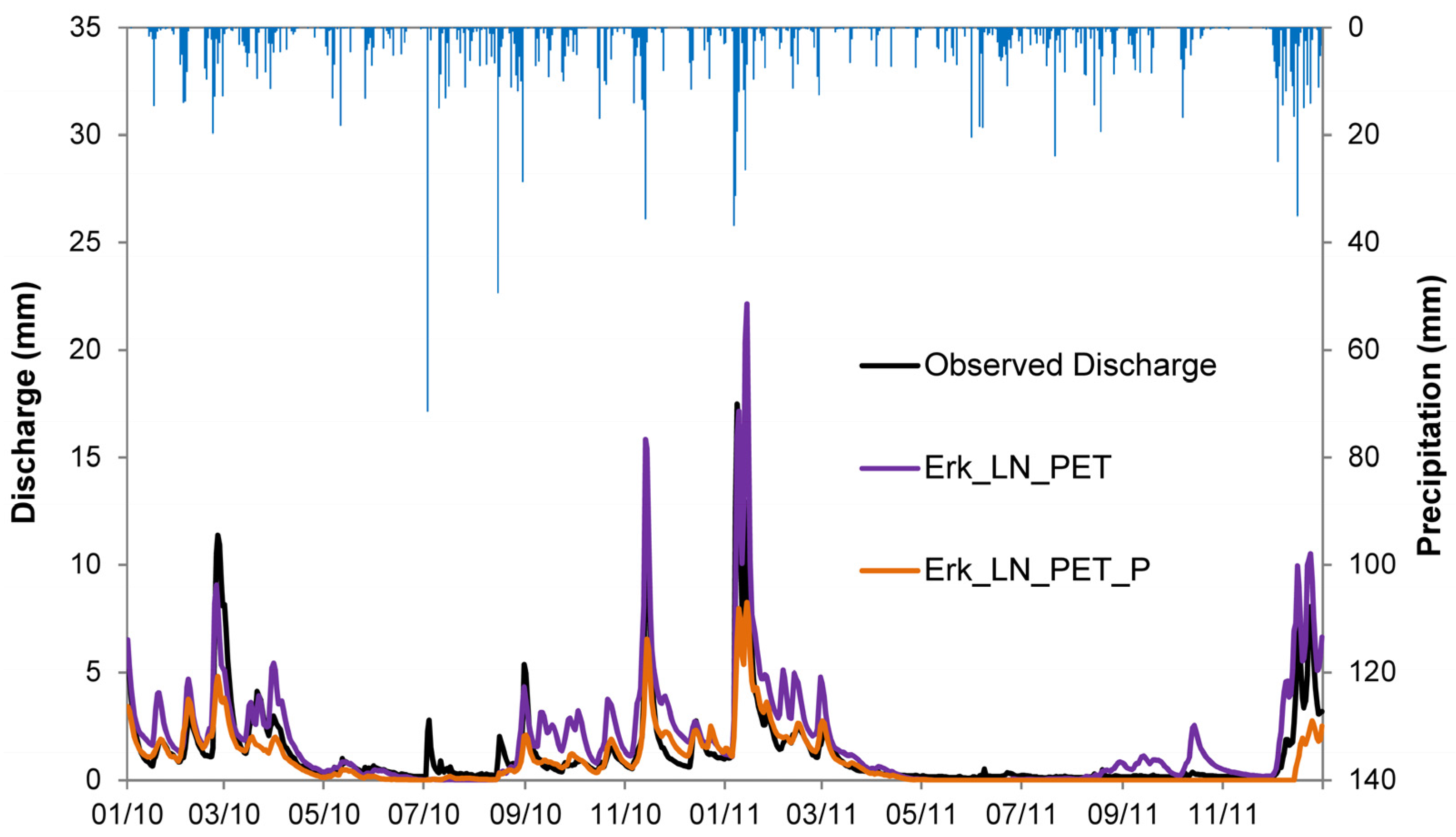
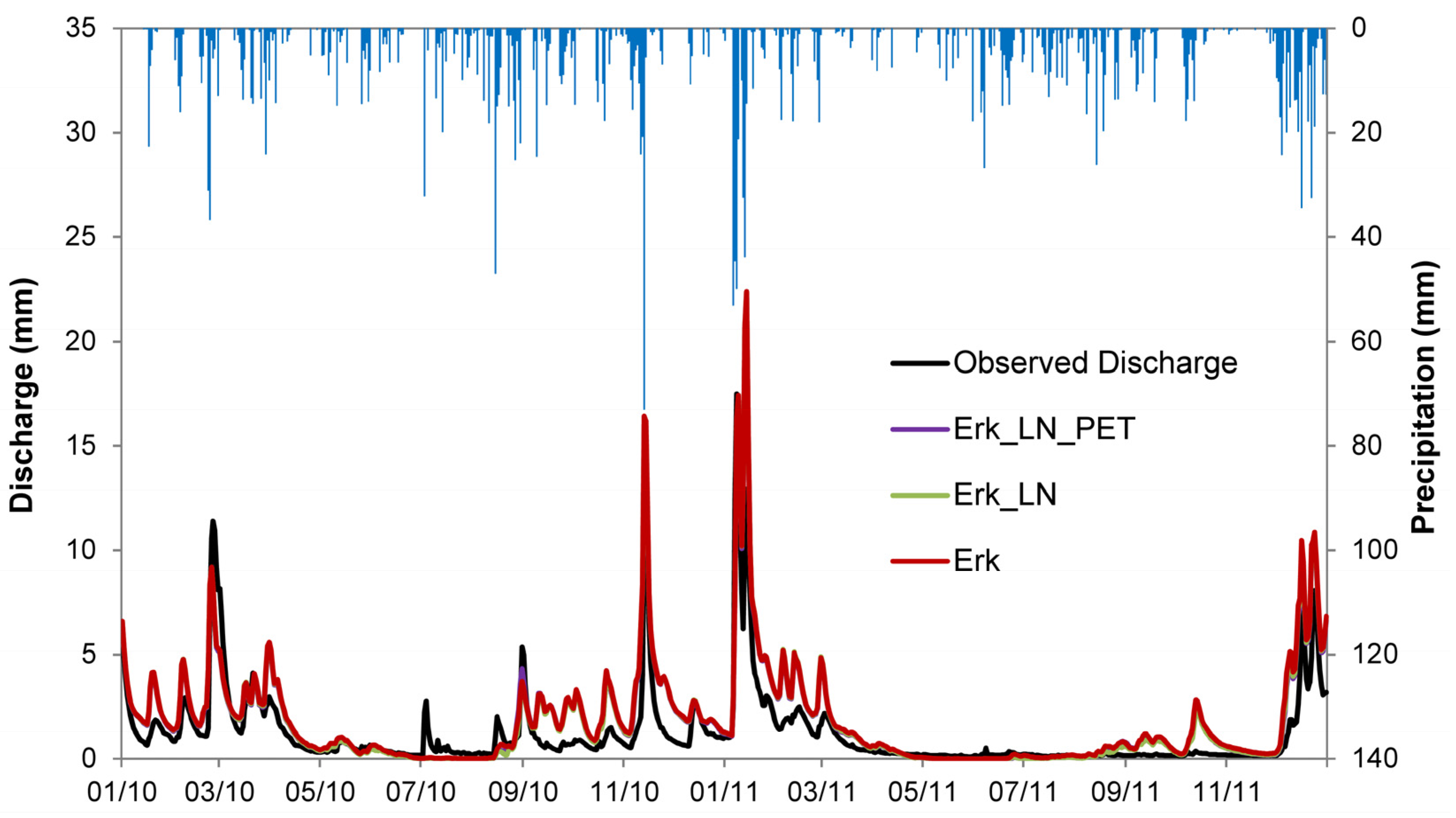
The three Erkensruhr simulations with homogeneous rainfall (Figure 6) heavily overestimated discharge amounts, especially during autumn because the applied rainfall originated from a climate station located in the southwestern—and thus wettest—part of the catchment. The usage of distributed precipitation substantially improved the discharge simulation of the Erkensruhr in terms of total sum, rising and falling limbs and low flows (Figure 7). However the discharge peaks were underestimated, possibly because the same interception and transpiration parameterization was used for a different precipitation input data set. We further found that using spatially aggregated instead of distributed radar precipitation data, produced equal simulation results in terms of water balance and discharge (not shown).

The overestimation of simulated discharge amounts at the Erkensruhr outlets caused bias values around 1.6 for the Erk model scenario during summer (Figure 8).

The R² values of the Erkensruhr simulations were considerably higher during winter (0.86) than during summer (0.22). As the R² during winter was higher for the Erkensruhr simulations than for the independent Wüstebach simulations (refer to Figure 3), we assumed that the snow model used in both simulations performed better for the smoother discharge curve of the mesoscale catchment. A plausible reason for this is a smoothing effect on winter discharges due to the larger catchment size.

The usage of distributed precipitation data mainly improved the bias during winter. During summer, distributed precipitation rates caused the bias to change from a 50% overestimation (Erk_LN_PET) to a 50% underestimation.

Evaporation amounts of the Erk simulation which considered spatially homogeneous coniferous land use throughout the catchment were slightly lower (by 15 mm) than that of Wbach and WbachEsoilConi, with the same land use type (refer to Table 4 and

Table 5. Water balance components for simulations of the Erkensruhr catchment.

	Simulation	Erk		Erk_LN		Erk_LN_PET		Erk_LN_PET_P
Water Balance Setup Component		2010	2011	2010	2011	2010	2011	2010	2011
Rainfall (mm)		1226	1348	1226	1348	1226	1348	956	902
Potential ET (mm)		694	756	694	756	694	757	694	757
Measured Discharge (mm)		524	396	524	396	524	396	524	396
Transpiration (mm)		226	272	268	286	260	305	283	332
Evaporation (mm)		265	289	278	306	288	312	265	267
Actual Evapotranspiration (mm)		491	561	546	592	548	617	548	599
Discharge (mm)		721	654	696	623	692	619	391	245
Infiltration (mm)		996	954	1024	980	1016	976	771	683

). The consideration of heterogeneous land use in the Erk_LN scenario slightly increased evaporation by 13 mm in 2010 and 17 mm in 2011. As already mentioned, the mesoscale soil data decreased simulated transpiration and infiltration amounts in the Wüstebach simulations independent of land use type. However transpiration of the Erk scenario was equal to that of the Wbach scenario and infiltration slightly increased.

The total evapotranspiration amount increased when heterogeneous land use information was used compared to the Erk setup. The consideration of distributed PET increased total evapotranspiration in 2011 by 25 mm with increases in both evapotranspiration components.

Reasons for the deviations in the water balance of the simulations Erk, Erk_LN, Erk_LN_PET are comparable to the Wüstebach simulations that have already been explained in Chapter 4.1.

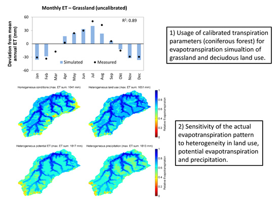
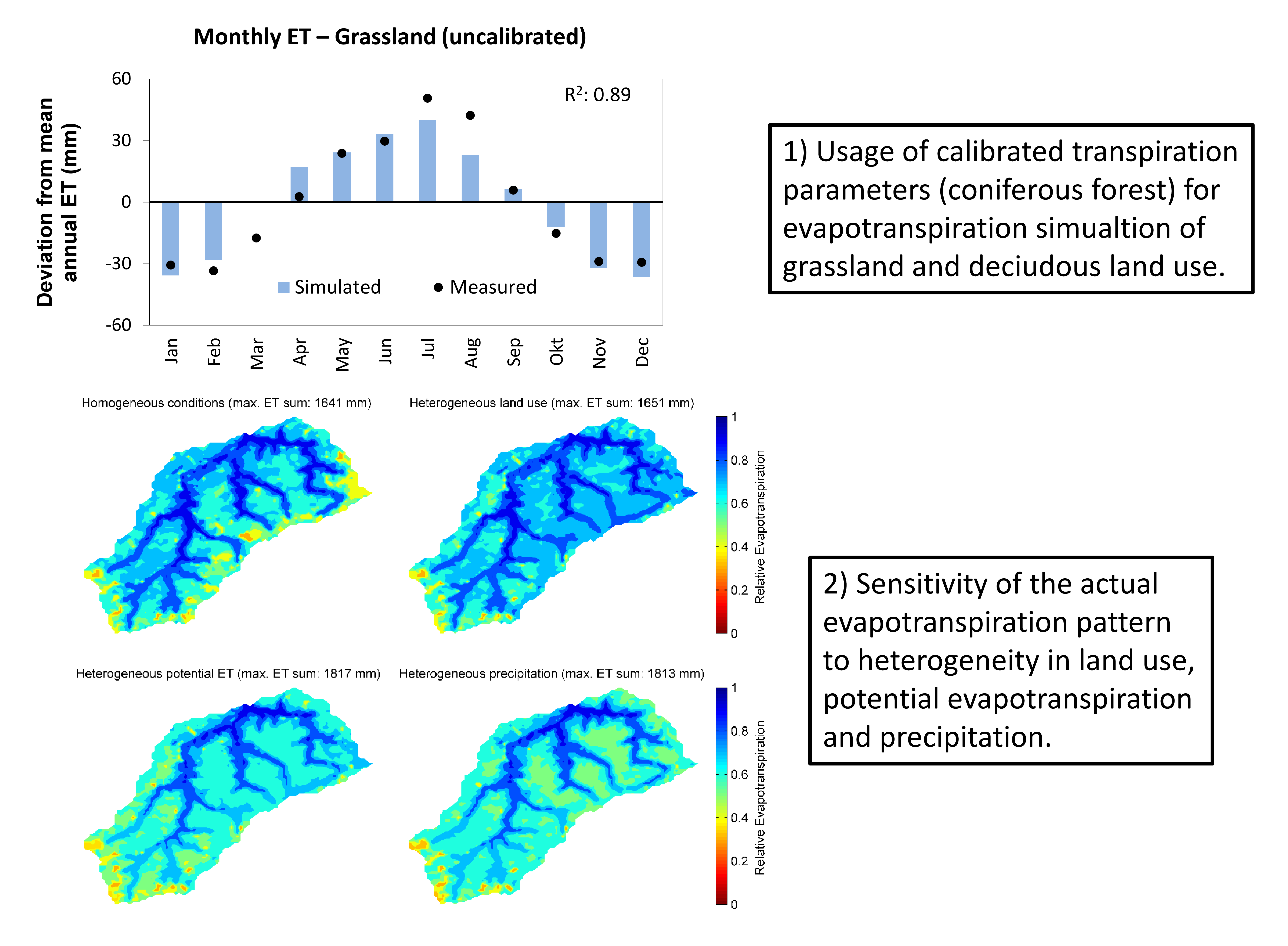
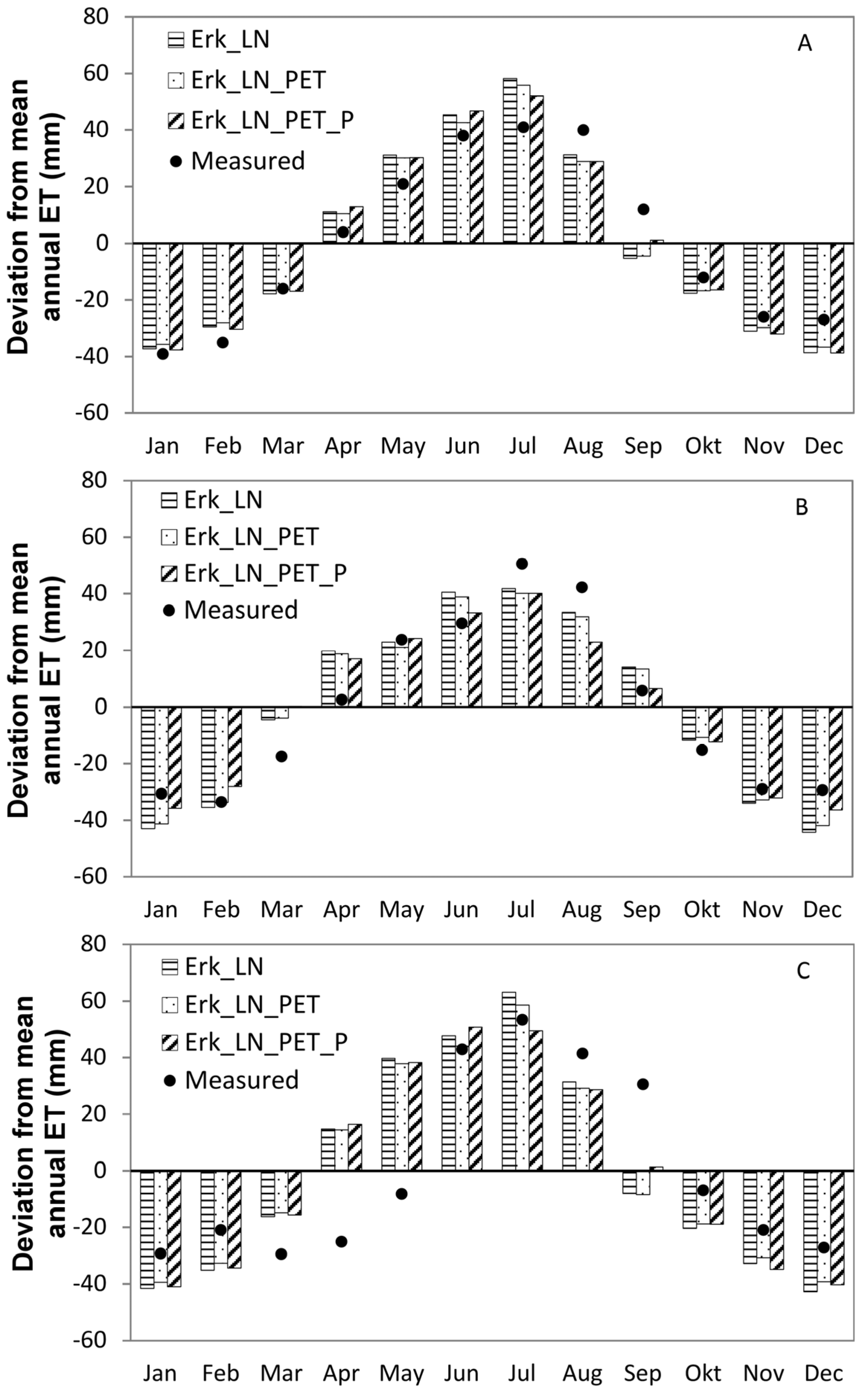
Figure 9 shows measured and simulated monthly deviations from mean annual evapotranspiration rates for coniferous (Figure 9A), grassland (Figure 9B) and deciduous (Figure 9C) vegetation. The simulated values were compared with measured eddy-covariance data in the case of coniferous and grassland vegetation; and to literature values from Mendel [45] in the case of deciduous vegetation.

For coniferous and grassland vegetation, the trend in mean monthly evapotranspiration was well simulated with R² values larger than 0.9. In the case of coniferous vegetation, the monthly evapotranspiration was overestimated between April and July and in December while it was underestimated in August, September and February. Distributed precipitation rates improved the simulation in July while the simulation Erk_LN_PET was the most unfavorable simulation meaning that PET was slightly underestimated for coniferous land use when the distribution method was used. Simulation of the evapotranspiration of the grassland vegetation was best during the winter and worst during March and April. For deciduous vegetation, Figure 9C reveals largest deviations between simulated and measured data taken from literature [45].

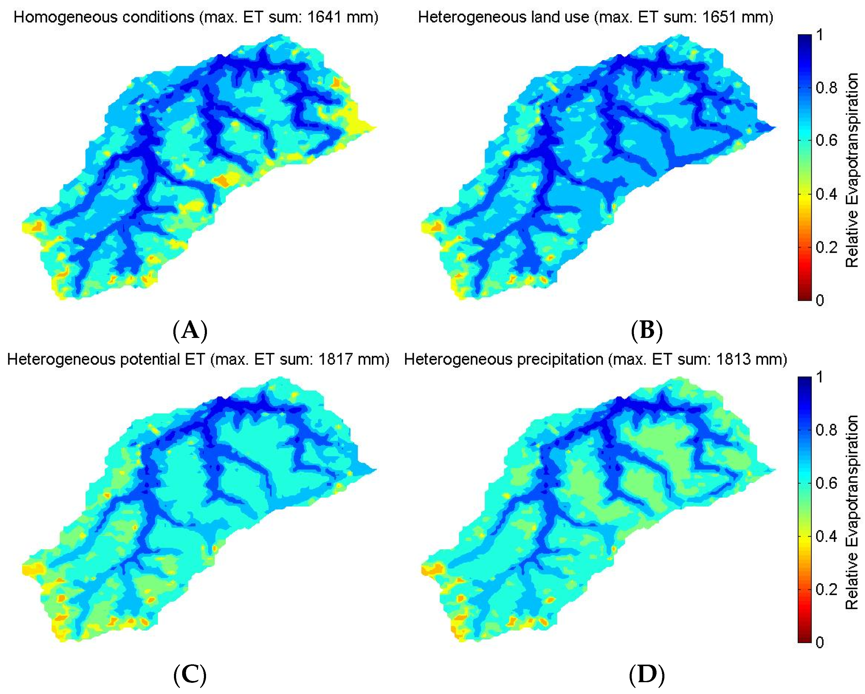
Figure 10 shows the pattern of simulated mean actual evapotranspiration given as a relative value of the sum of evapotranspiration for 2010 and 2011. The pattern of the Erk scenario (Figure 10A), shows a clearly defined riparian and stream area with very high relative evapotranspiration values close to unity. Driest conditions were found at the ridge of hills at the eastern, western and southern borders of the catchment. The pattern shown in Figure 10B for the Erk_LN scenario, illustrates that the incorporation of heterogeneous land use enhanced evapotranspiration in the central part of the catchment covered with grassland. Distributed PET decreased actual evapotranspiration in higher parts of the catchments (e.g., south-western border). The incorporation of distributed precipitation generally decreased the contribution of grassland areas.

4. Discussion

4.1. Influence of Mesoscale Soil and Land Use Parameterization on the Simulation of the Headwater Catchment

Results of the Wüstebach simulations revealed a strong influence of (1) soil data on runoff generating processes and of (2) land use parameterization on evapotranspiration components.

The observed increase in fast runoff components due to an increase in saturated conductivity, led to a unique interplay between antecedent wetness, infiltration, groundwater level rise and transpiration parameterization which strongly depended on the difference between precipitation and PET during spring.

This observed high sensitivity of fast runoff sums and runoff generation mechanisms to changes in soil properties agreed well with the findings of many studies; but the result that higher saturated conductivity led to an increase in fast runoff components contradicted to results reported in the literature for simulations with distributed hydrological models [47,48,49].

The applicability of mesoscale land use parameterization was validated with a comparison between evapotranspiration amounts simulated with Wüstebach soil data (Table 4) and values reported in the literature.

Simulated evapotranspiration of grassland amounted to 46% of total catchment rainfall but literature values ranged between 36% of 800 mm precipitation for a measurement site in Germany [50] and 60% of total rainfall at a grassland site near to the Erkensruhr catchment (Schmidt, personal communication). Data cited in Mendel [45] ranged between 55% of 800 mm precipitation and 75% of only 581 mm precipitation).

Despite the lack of calibration, simulated interception fractions for the deciduous forest (17% of total precipitation) corresponded well to the value reported by Oishi et al. [51] for a hardwood forest in the United States with a precipitation of 1091 mm. Mendel [45] reported interception values between 5% and 48% of precipitation for a beech forest. Simulated fractions of evapotranspiration (without interception) amounted to 25% but literature values ranged between 26% [45] and 40% [51] of catchment rainfall.

The broad range of reported evapotranspiration components for both land uses pointed to considerable uncertainty in evapotranspiration validation thus expressing the need for additional land use specific evapotranspiration measurements.

4.2. Influence of Parameter Regionalization and Spatially Distributed Input Data on the Simulation of the Mesoscale Catchment

Erkensruhr simulations revealed that the quality of the discharge simulation in terms of dynamics, amount and peak flow rates, was most sensitive to differences in precipitation data. Spatially distributed land use parameterization only affected discharge amounts while spatially distributed PET had a weak effect on discharge but a significant effect on the pattern of actual evapotranspiration during winter (not shown).

An influence of spatial precipitation patterns on hydrological simulations has been long under debate. For example, Schuurmans and Bierkens [52] and Arnaud et al. [53] compared simulation results of distributed models using spatially distributed and spatially aggregated precipitation input. Schuurmans and Bierkens [52] found that spatial variability of rainfall is necessary to simulate spatial variability in daily discharge, groundwater level and soil moisture content but not required for aggregated measures like catchment mean groundwater table or water balance. Arnaud et al. [53] showed at two mesoscale catchments (103 and 22 km²), that differences in simulated discharge amount and peak flow rates decreased with increasing peak flow rate. In our study, differences in discharge rates between simulations with aggregated and spatially distributed precipitation were therefore marginally supporting the results from Schuurmans and Bierkens [52], that spatially distributed precipitation is not required for the correct simulation of aggregated measures of hydrologic functioning, like the water balance. In contrast to Schuurmans and Bierkens [52], simulated evapotranspiration patterns were similar between simulations with aggregated and distributed precipitation, indicating that the spatial evapotranspiration simulation in HGS is more sensitive to parameterization than precipitation data. The high sensitivity of peak flow rates to precipitation sum and distribution highlights the extraordinary importance of meteorological forcing data in comparison to parameterization efforts.

Mean monthly evapotranspiration was well simulated at the mesoscale catchment for coniferous forest and grassland (R²: 0.9) and to a lesser degree for deciduous vegetation (R²: 0.58) as the data used were book values and therefore the most unreliable [45]. Interestingly, the simulated trend improved when values were re-shifted in positive direction by one month, giving an R² of 0.88 revealing a systematic error in MODIS LAI data and/or measured evapotranspiration data from Mendel [45]. The results indicated that usage of the same model-specific transpiration parameters for different land uses can be sufficient to reproduce monthly dynamics of evapotranspiration.

We acknowledge that the presented results originated from a study of two catchments with similar catchment properties. To allow for a more general evaluation of our parameter transfer approach, applications to further catchments with different catchment properties, e.g., in terms of topography, soil properties, geology, climate etc. will need to be made. Such an analysis would also help to define the limits of our model parameter transfer approach.

5. Conclusions

In this study, we dealt with one of the major limitations to the application of distributed hydrological models at mesoscale catchments: the commonly available data base at mesoscale catchments is insufficient for a thorough calibration and validation. We parameterized the distributed hydrological model HydroGeoSphere for a mesoscale catchment by transferring model-specific parameters calibrated for water balance and soil moisture dynamics at a small headwater catchment. To account for the spatial variability in land use at the mesoscale catchment, parameters that are not model-specific (e.g., LAI, root depth and distribution) were taken from the literature.

At the mesoscale, the effect of transferred parameterization was differentiated from the influence of spatial variability in soil, land use, potential evapotranspiration and precipitation by a step-wise introduction of their spatial distributions into the model setup. In addition, the possible range of model behavior was exploited by using mesoscale soil and land use data for the simulation of the headwater catchment.

Using mesoscale soil data from the mesoscale catchment in the headwater simulation revealed a model specific behavior, as higher saturated conductivities enhanced faster runoff components instead of reducing them, as reported in the literature [47,48,49]. We attributed this finding to a unique interplay between wetness prior to rainfall events during the summer, groundwater level rise and transpiration parameterization.

The mesoscale simulations with regionalized model-specific parameters reproduced discharge dynamics and evapotranspiration in a satisfying manner. Precipitation was the most sensitive input data set for discharge simulation, while spatially distributed land use parameterization had a much larger effect on evapotranspiration components and its pattern, than distributed precipitation or potential evapotranspiration.

References

1. Panday, S.; Huyakorn, P.S. A fully coupled physically-based spatially-distributed model for evaluating surface/subsurface flow. Adv. Water Resour. 2004, 27, 361–382. [Google Scholar] [CrossRef]
2. Kollet, S.J.; Maxwell, R.M. Capturing the influence of groundwater dynamics on land surface processes using an integrated, distributed watershed model. Water Resour. Res. 2008, 44, W02402. [Google Scholar] [CrossRef]
3. Graham, D.N.; Butts, M.B. Flexible, integrated watershed modelling with MIKE SHE. In Watershed Models; Singh, V.P., Frevert, D.K., Eds.; CRC Press: Boca Raton, FL, USA, 2005; pp. 245–271. [Google Scholar]
4. Camporese, M.; Paniconi, C.; Putti, M.; Orlandini, S. Surface-subsurface flow modeling with path-based runoff routing, boundary condition-based coupling, and assimilation of multisource observation data. Water Resour. Res. 2010, 46, W02512. [Google Scholar] [CrossRef]
5. Ala-aho, P.; Rossi, P.M.; Isokangas, E.; Kløve, B. Fully integrated surface-subsurface flow modelling of groundwater–lake interaction in an esker aquifer: Model verification with stable isotopes and airborne thermal imaging. J. Hydrol. 2015, 522, 391–406. [Google Scholar] [CrossRef]
6. Frei, S.; Fleckenstein, J.H. Representing effects of micro-topography on runoff generation and sub-surface flow patterns by using superficial rill/depression storage height variations. Environ. Model. Softw. 2014, 52, 5–18. [Google Scholar] [CrossRef]
7. Li, Q.; Unger, A.J.A.; Sudicky, E.A.; Kassenaar, D.; Wexler, E.J.; Shikaze, S. Simulating the multi-seasonal response of a large-scale watershed with a 3D physically-based hydrologic model. J. Hydrol. 2008, 357, 317–336. [Google Scholar] [CrossRef]
8. Voeckler, H.M.; Allen, D.M.; Alila, Y. Modeling coupled surface water—Groundwater processes in a small mountainous headwater catchment. J. Hydrol. 2014, 517, 1089–1106. [Google Scholar] [CrossRef]
9. Weill, S.; Altissimo, M.; Cassiani, G.; Deiana, R.; Marani, M.; Putti, M. Saturated area dynamics and streamflow generation from coupled surface-subsurface simulations and field observations. Adv. Water Resour. 2013, 59, 196–208. [Google Scholar] [CrossRef]
10. Kirchner, J.W. Getting the right answers for the right reasons: Linking measurements, analyses, and models to advance the science of hydrology. Water Resour. Res. 2006, 42, W03S04. [Google Scholar] [CrossRef]
11. Liang, X.; Lettenmaier, D.P.; Wood, E.F.; Burges, S.J. A simple hydrologically based model of land surface water and energy fluxes for general circulation models. J. Geophys. Res. Atmos. 1994, 99, 14415–14428. [Google Scholar] [CrossRef]
12. Troy, T.J.; Wood, E.F.; Sheffield, J. An efficient calibration method for continental-scale land surface modeling. Water Resour. Res. 2008, 44, W09411. [Google Scholar] [CrossRef]
13. Romano, N. Soil moisture at local scale: Measurements and simulations. J. Hydrol. 2014, 516, 6–20. [Google Scholar] [CrossRef]
14. Graf, A.; Bogena, H.R.; Drüe, C.; Hardelauf, H.; Pütz, T.; Heinemann, G.; Vereecken, H. Spatiotemporal relations between water budget components and soil water content in a forested tributary catchment. Water Resour. Res. 2014, 50, 4837–4857. [Google Scholar] [CrossRef]
15. Cornelissen, T.; Diekkrüger, B.; Bogena, H.R. Significance of scale and lower boundary condition in the 3D simulation of hydrological processes and soil moisture variability in a forested headwater catchment. J. Hydrol. 2014, 516, 140–153. [Google Scholar] [CrossRef]
16. Goderniaux, P.; Brouyère, S.; Fowler, H.J.; Blenkinsop, S.; Therrien, R.; Orban, P.; Dassargues, A. Large scale surface-subsurface hydrological model to assess climate change impacts on groundwater reserves. J. Hydrol. 2009, 373, 122–138. [Google Scholar] [CrossRef]
17. Rahman, M.; Sulis, M.; Kollet, S.J. The concept of dual-boundary forcing in land surface-subsurface interactions of the terrestrial hydrologic and energy cycles. Water Resour. Res. 2014, 50, 8531–8548. [Google Scholar] [CrossRef]
18. Hauck, C.; Barthlott, C.; Krauss, L.; Kalthoff, N. Soil moisture variability and its influence on convective precipitation over complex terrain. Q. J. R. Meteorol. Soc. 2011, 137, 42–56. [Google Scholar] [CrossRef]
19. Bogena, H.R.; Diekkrüger, B. Modelling solute and sediment transport at different spatial and temporal scales. Earth Surf. Process. Landf. 2002, 27, 1475–1489. [Google Scholar] [CrossRef]
20. Moriasi, D.N.; Arnold, J.G.; Van Liew, M.W.; Bingner, R.L.; Harmel, R.D.; Veith, T.L. Model evaluation guidelines for systematic quantification of accuracy in watershed simulations. Trans. ASABE 2007, 50, 885–900. [Google Scholar] [CrossRef]
21. Stoltidis, I.; Krapp, L. Hydrological Map NRW. 1:25.000, Sheet 5404; State Agency for Water and Waste of North Rhine-Westfalia: Düsseldorf, Germany, 1980. [Google Scholar]
22. Stockinger, M.P.; Bogena, H.R.; Lücke, A.; Diekkrüger, B.; Weiler, M.; Vereecken, H. Seasonal soil moisture patterns: Controlling transit time distributions in a forested headwater catchment. Water Resour. Res. 2014, 50, 5270–5289. [Google Scholar] [CrossRef]
23. Bogena, H.R.; Herbst, M.; Huisman, J.A.; Rosenbaum, U.; Weuthen, A.; Vereecken, H. Potential of Wireless Sensor Networks for Measuring Soil Water Content Variability. Vadose Zone J. 2010, 9, 1002–1013. [Google Scholar] [CrossRef]
24. Lehmkuhl, F.; Loibl, D.; Borchardt, H. Geomorphological map of the Wüstebach (Nationalpark Eifel, Germany)—An example of human impact on mid-European mountain areas. J. Maps 2010, 6, 520–530. [Google Scholar] [CrossRef]
25. Bogena, H.R.; Bol, R.; Borchard, N.; Brüggemann, N.; Diekkrüger, B.; Drüe, C.; Groh, J.; Gottselig, N.; Huisman, J.A.; Lücke, A.; et al. A terrestrial observatory approach to the integrated investigation of the effects of deforestation on water, energy, and matter fluxes. Sci. China Earth Sci. 2015, 58, 61–75. [Google Scholar] [CrossRef]
26. Aquanty. HGS 2013: HydroGeoSphere—User Manual; Aquanty: Waterloo, ON, Canada, 2013. [Google Scholar]
27. Hwang, H.-T.; Park, Y.-J.; Sudicky, E.A.; Forsyth, P.A. A parallel computational framework to solve flow and transport in integrated surface–subsurface hydrologic systems. Environ. Model. Softw. 2014, 61, 39–58. [Google Scholar] [CrossRef]
28. Kristensen, K.J.; Jensen, S.E. A model for estimating actual evapotranspiration form potential evapotranspiration. Nord. Hydrol. 1975, 6, 170–188. [Google Scholar]
29. Partington, D.; Brunner, P.; Frei, S.; Simmons, C.T.; Werner, A.D.; Therrien, R.; Maier, H.R.; Dandy, G.C.; Fleckenstein, J.H. Interpreting streamflow generation mechanisms from integrated surface-subsurface flow models of a riparian wetland and catchment. Water Resour. Res. 2013, 49, 5501–5519. [Google Scholar] [CrossRef]
30. Allen, R.G.; Pereira, L.S.; Raes, D.; Smith, M. FAO Irrigation and Drainage Paper No. 56; FAO: Rome, Italy, 1998. [Google Scholar]
31. Breuer, L.; Eckhardt, K.; Frede, H.-G. Plant parameter values for models in temperate climates. Ecol. Model. 2003, 169, 237–293. [Google Scholar] [CrossRef]
32. Richter, D. Ergebnisse Methodischer Untersuchungen zur Korrektur des Systematischen Meßfehlers des Hellmann-Niederschlagsmessers. Berichte des Deutschen Wetterdienstes; German Weather Service: Offenbach am Main, Germany, 1995. [Google Scholar]
33. Maidment, D. Handbook of Hydrology; McGraw-Hill: New York, NY, USA, 1993. [Google Scholar]
34. Waldhoff, G. Enhanced Land Use Classification of 2008 for the Rur Catchment; CRC/TR32 Database (TR32DB), doi:10.5880/TR32DB.1; University of Cologne: Cologne, Germany, 2012. [Google Scholar]
35. Van Genuchten, M.T. A closed-form equation for predicting the hydraulic conductivity of unsaturated soils. Soil Sci. Soc. Am. J. 1980, 44, 892–898. [Google Scholar] [CrossRef]
36. Rawls, W.J.; Brakensiek, D.L. Prediction of soil water properties for hydrologic modeling. In Proceedings of the Symposium Watershed Management in the Eighties, Denver, CO, USA, 30 April–1 May 1985; pp. 293–399.
37. Brakensiek, D.L.; Rawls, W.J. Soil containing rock fragments: Effects on infiltration. Catena 1994, 23, 99–110. [Google Scholar] [CrossRef]
38. Bogena, H.R.; Huisman, J.A.; Baatz, R.; Hendricks Franssen, H.-J.; Vereecken, H. Accuracy of the cosmic-ray soil water content probe in humid forest ecosystems: The worst case scenario: Cosmic-Ray Probe in Humid Forested Ecosystems. Water Resour. Res. 2013, 49, 5778–5791. [Google Scholar] [CrossRef]
39. Brakensiek, D.L.; Rawls, W.J.; Stephenson, G.R. Determining the Saturated Hydraulic Conductivity of a Soil Containing Rock Fragments. Soil Sci. Soc. Am. J. 1986, 50, 834–835. [Google Scholar] [CrossRef]
40. Sciuto, G.; Diekkrüger, B. Influence of soil heterogeneity and spatial discretization on catchment water balance modeling. Vadose Zone J. 2010, 9, 955–969. [Google Scholar] [CrossRef]
41. Meinen, C.; Hertel, D.; Leuschner, C. Biomass and morphology of fine roots in temperate broad-leaved forests differing in tree species diversity: Is there evidence of below-ground overyielding? Oecologia 2009, 161, 99–111. [Google Scholar] [CrossRef] [PubMed]
42. Dannowski, M.; Wurbs, A. Spatial differentiated representation of maximum rooting depths of different plant communities on a field wood-area of the Northeast German Lowland. Bodenkultur 2003, 54, 93–108. [Google Scholar]
43. Beven, K.J. Rainfall-Runoff Modelling—The Primer; Wiley: Chichester, UK, 2001. [Google Scholar]
44. Rosenbaum, U.; Bogena, H.R.; Herbst, M.; Huisman, J.A.; Peterson, T.J.; Weuthen, A.; Western, A.W.; Vereecken, H. Seasonal and event dynamics of spatial soil moisture patterns at the small catchment scale. Water Resour. Res. 2012, 48, W10544. [Google Scholar] [CrossRef]
45. Mendel, H. Elemente des Wasserkreislaufs: Eine Kommentierte Bibliographie zur Abflußbildung; Analytica: Berlin, Germany, 2000. [Google Scholar]
46. Qu, W.; Bogena, H.R.; Huisman, J.A.; Vanderborght, J.; Schuh, M.; Priesack, E.; Vereecken, H. Predicting subgrid variability of soil water content from basic soil information: Predict soil water content variability. Geophys. Res. Lett. 2015, 42, 789–796. [Google Scholar] [CrossRef]
47. Bormann, H.; Breuer, L.; Gräff, T.; Huisman, J.A. Analysing the effects of soil properties changes associated with land use changes on the simulated water balance: A comparison of three hydrological catchment models for scenario analysis. Ecol. Model. 2007, 209, 29–40. [Google Scholar] [CrossRef]
48. Herbst, M.; Diekkrüger, B.; Vanderborght, J. Numerical experiments on the sensitivity of runoff generation to the spatial variation of soil hydraulic properties. J. Hydrol. 2006, 326, 43–58. [Google Scholar] [CrossRef]
49. Kværnø, S.H.; Stolte, J. Effects of soil physical data sources on discharge and soil loss simulated by the LISEM model. CATENA 2012, 97, 137–149. [Google Scholar] [CrossRef]
50. Harsch, N.; Brandenburg, M.; Klemm, O. Large-scale lysimeter site St. Arnold, Germany: Analysis of 40 years of precipitation, leachate and evapotranspiration. Hydrol. Earth Syst. Sci. 2009, 13, 305–317. [Google Scholar] [CrossRef]
51. Oishi, A.C.; Oren, R.; Stoy, P.C. Estimating components of forest evapotranspiration: A footprint approach for scaling sap flux measurements. Agric. For. Meteorol. 2008, 148, 1719–1732. [Google Scholar] [CrossRef]
52. Schuurmans, J.M.; Bierkens, M.F.P. Effect of spatial distribution of daily rainfall on interior catchment response of a distributed hydrological model. Hydrol. Earth Syst. Sci. Discuss. 2007, 11, 677–693. [Google Scholar] [CrossRef]
53. Arnaud, P.; Bouvier, C.; Cisneros, L.; Dominguez, R. Influence of rainfall spatial variability on flood prediction. J. Hydrol. 2002, 260, 216–230. [Google Scholar] [CrossRef]
Figure 1. Location of the Erkensruhr catchment and climate stations (A); land use (B) and soil type distribution in the Erkensruhr catchment (C). The bottom map also illustrates the border between the slope of the hill and the riparian area (refer to Chapter 2.3).
Water 08 00202 g001
Figure 2. (A) Comparison of observed and simulated discharge of the Wüstebach for simulations with high-resolution soil data (Wbach) and low-resolution soil data (WbachEsoilConi); (B) Discharge difference between simulations with changing land use; (C) Discharge difference between simulations with changing land use and soil data.
Water 08 00202 g002
Figure 3. Bias (black line), coefficient of variation (CV; green line) and correlation coefficient (red line) in hydrological summer (solid lines) and winter (dashed lines) for the Wüstebach discharge simulations.
Water 08 00202 g003
Figure 4. Soil moisture dynamics of the Wüstebach simulations at 20 cm depth.
Water 08 00202 g004
Figure 5. Relationship between mean soil moisture and its standard deviation for Wüstebach simulations at 5 cm depth with (A) Wüstebach and (B) Erkensruhr soil data.
Water 08 00202 g005
Figure 6. Observed and simulated discharge of the Erkensruhr for simulations with heterogeneous soil data (Erk), heterogeneous soil and land use data (Erk_LN), heterogeneous soil, land use and potential evapotranspiration data (Erk_LN_PET).
Water 08 00202 g006
Figure 7. Observed and simulated discharge of the Erkensruhr for simulations with homogeneous (Erk_LN_PET) and distributed precipitation (Erk_LN_PET_P).
Water 08 00202 g007
Figure 8. Bias (black line), coefficient of variation (CV; green line) and correlation coefficient (red line) in hydrological summer (solid lines) and winter (dashed lines) for the Erkensruhr discharge simulations.
Water 08 00202 g008
Figure 9. Measured and simulated monthly deviation from mean annual evapotranspiration rates for (A) coniferous; (B) grassland and (C) deciduous vegetation. Measured data refer to (A) eddy-covariance data from [14]; (B) eddy-covariance data from Schmidt (personal communication) and; (C) mean monthly data from a low mountain catchment in northern Germany between 1969 and 1972 with a mean rainfall of 1066 mm [45].
Water 08 00202 g009
Figure 10. Pattern of actual evapotranspiration for simulations Erk (A), Erk_LN (B), Erk_LN_PET (C) and Erk_LN_PET_P (D). Evapotranspiration is given relative to the maximum of the actual evapotranspiration sums of 2010 and 2011 as specified in the brackets.
Water 08 00202 g010