A Novel Water Supply Network Sectorization Methodology Based on a Complete Economic Analysis, Including Uncertainties

Abstract

The core idea behind sectorization of Water Supply Networks (WSNs) is to establish areas partially isolated from the rest of the network to improve operational control. Besides the benefits associated with sectorization, some drawbacks must be taken into consideration by water operators: the economic investment associated with both boundary valves and flowmeters and the reduction of both pressure and system resilience. The target of sectorization is to properly balance these negative and positive aspects. Sectorization methodologies addressing the economic aspects mainly consider costs of valves and flowmeters and of energy, and the benefits in terms of water saving linked to pressure reduction. However, sectorization entails other benefits, such as the reduction of domestic consumption, the reduction of burst frequency and the enhanced capacity to detect and intervene over future leakage events. We implement a development proposed by the International Water Association (IWA) to estimate the aforementioned benefits. Such a development is integrated in a novel sectorization methodology based on a social network community detection algorithm, combined with a genetic algorithm optimization method and Monte Carlo simulation. The methodology is implemented over a fraction of the WSN of Managua city, capital of Nicaragua, generating a net benefit of 25,572 $/year.

1. Introduction

Sectorization of Water Supply Networks (WSNs) can be described as a technique aimed at improving WSN operational control, including, among others, leakage and pressure management, monitoring of water quality, speeding upof repairing activities and the definition of supply schedules in WSNs with intermittent supply. The core idea is to establish areas partially isolated from the rest of the network. Such isolation is carried out either by means of closing valves/cutting pipes, in the case of static sectorizations, or by means of dynamically-operated valves, in the case of dynamic sectorizations [1]. Once an area is isolated, it is supplied either by one single entrance or by several entrances. In either case, each entrance must be equipped with a Control operation Unit (CU). A CU should be constructed around the entrance pipe and must count on at least one flowmeter, in order to be able to permanently control the inlet flow (also pressure and/or physical/chemical parameters can be monitored). The CU needs to have enough space for maintenance activities and, also, should be able to support traffic loads.

Besides the aforementioned benefits, the sectorization of WSNs has some drawbacks, namely the required economic investment for the purchase and installation of both boundary valves and CUs and the reduction of the overall pressure due to the closure of some pipes, which also increases the energy consumption. Although pressure reduction entails benefits in terms of leakage flow reduction, it can also lead to partial or temporal shortages.

The target pursued when a sectorization layout is designed is to properly balance the negative and positive aspects described above. This is achieved by the optimal location of both valves and CUs. As expected, the number of possible combinations CU/boundary valves grows combinatorially with the pipe extension and the network meshing configuration [2,3], which makes unfeasible any manual design and makes necessary the use of mathematical and computational techniques.

Depending on the network topology, sectorization can be conducted in two ways: if the network counts on many sources and these are located within the meshing space, the sectors can be established around the sources; on the contrary, when the number of sources is limited and/or they are located outside the meshing area, the network has to be supplied by a main conduction system (or trunk network), and therefore, the sectors have to be established around the latter. In this work, we address this last case. To identify the trunk network, a method proposed in [4] is implemented. This method is based on a combination of the short path concept from graph theory and on hydraulic simulation.

Once the trunk network is defined, it is uncoupled from the distribution network. This step is important in order to keep the connectivity of the first, thus preserving the flexibility of the entire supply system and also reducing the budget for the acquisition of CUs and boundary valves. Over the distribution network, a multilevel community detection algorithm [5] is implemented. The communities generated by this algorithm are recursively merged in a fusion process herein proposed, until a partition in which each sector satisfies certain predetermined constraints is found.

Appropriate sectorization of WSNs has become a subject of interest for many researches in the last decade. Most of these studies have addressed the problem using graph theory and energy criteria [6,7,8] in combination with multi-agent systems [9,10], with heuristic optimization approaches [11,12,13] and, more recently, with concepts derived from social network theory [5,14,15].

In all of the cases, only the costs related to valves and CUs, the energy costand the benefits in terms of background leakages, linked to the reduction of pressure, are considered. However, such benefits are not too far from those that would be obtained only by following a pressure regulation strategy. When a WSN is sectorized, there are other benefits that can also be taken into consideration: the reduction of domestic consumption, the reduction of bursts and the enhanced capacity to detect and intervene over future leakage events, indistinctly if they are visually detectable or not. As explained below, this enhancement of the control capacity translates into the shortest detection and operation periods, thus reducing the annual volume of leakage and, hence, the operational costs.

Unfortunately, there is a lack of mathematical formulations to directly compute the relation among sectorization and all of the previously mentioned benefits. However, the International Water Association (IWA) has proposed a framework to estimate the benefits of pressure reduction [16], which we combine with a Genetic Algorithm (GA)-based optimization procedure in order to calculate part of the benefits of the sectorization. Additionally, we implement Monte Carlo Simulation (MCS) to include the benefit in terms of the speed of leakage event detection and pipe repairing within the optimization. For each iteration of the optimization algorithm that results in a feasible solution, an MCS is carried out, and the balance costs/benefits is updated. To the authors’ knowledge, this is the first research work related to sectorization that combines the optimization of the sectors’ layout with the leakage management concepts proposed by the IWA. Furthermore, it is the first work that includes the analysis of future leakage events and MCS. We hope that these ideas will be useful for future research focusing on the economic analysis of sectorization.

The rest of this paper is structured as follows: in the first part of Section 2 (Subsection 2.1), the algorithm that is used to segregate the trunk network and to define the sectors over the distribution network is described; in the second part (Subsection 2.2) of the same section, the proposed method to optimize the arrangement CUs/boundary valves is described. In the first three subsections, the concepts on leakage management, proposed by the IWA, are described; in Subsection 2.2.4, the objective function to be optimized is presented; finally, in Subsection 2.2.5, the use of MCS to predict the enhancement of the capacity to detect new leakage events is explained. Section 3 contains a description and analysis of the results obtained by implementing the methodology in a section of the WSN of Managua City, capital of Nicaragua. Such a description includes a table containing the economic benefits and costs of investments. Finally, in Section 4, the conclusions are presented.

2. Materials and Methods

2.1. Sector Definition Algorithm

Graphs are virtual structures topologically formed by nodes (or vertices) and links (or edges) that can be used to represent any kind of network, either physical or virtual. Graph theory is a branch of mathematics devoted to the study of these structures. WSNs can be represented as graphs, and over them, it is possible to implement algorithms of the graph theory domain. Two concepts of major importance from this theory are the “shortest path” between nodes and “community detection”. The first one allows finding the most efficient way to reach one node from any other, and the second one allows finding modules with a high level of cohesion that are separated from other modules by a minimized number of edges.

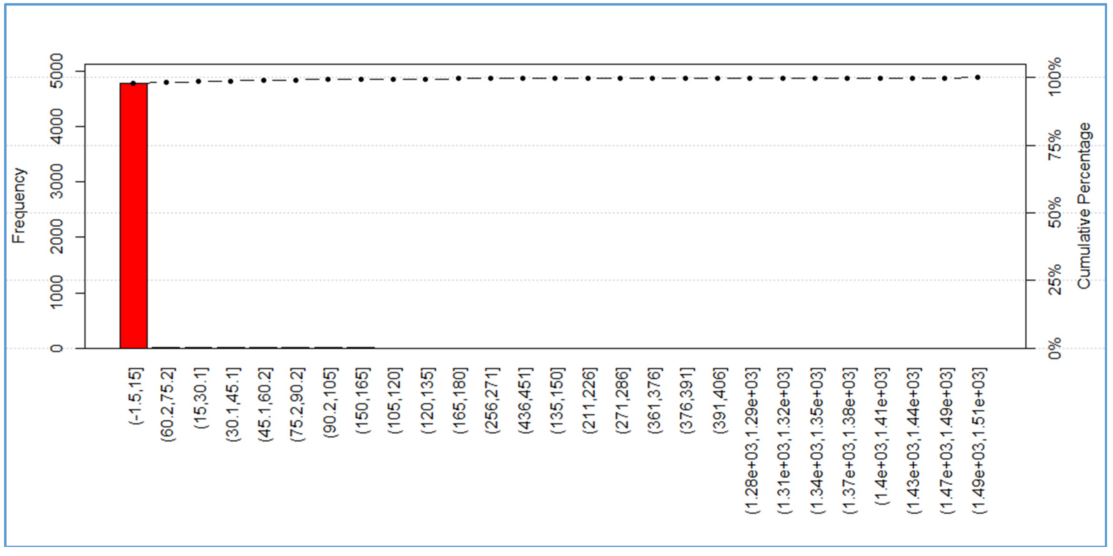
As previously mentioned, in this paper, the shortest path concept is used to define and segregate the trunk network from the distribution network; in this process, a ranking of pipes is generated. Such a ranking is based on the pipe’s role in the supply of the entire network. To assess the role of each pipe in the supply, a hydraulic simulation is conducted with EPANET for the most critical scenario (the instant of highest demand). Then, the direction of the flow in each pipe is retrieved and stored in a squared matrix. This matrix allows calculating the number of nodes/pipes that can be reached from every node, this being the Accumulated Shortest Path Value (ASPV). Then, the flow in each pipe is multiplied by its corresponding ASPV (the result is represented by AVSP*). The trunk network is expected to be formed by pipes with high and less frequent AVSP* values, whereas the pipes in the distribution network are expected to have low and highly frequent AVSP* values. This can be more clearly seen in Figure 1, where the tallest red bar represents almost 97% of the pipes having values of ASPV* in the same range (0–15). 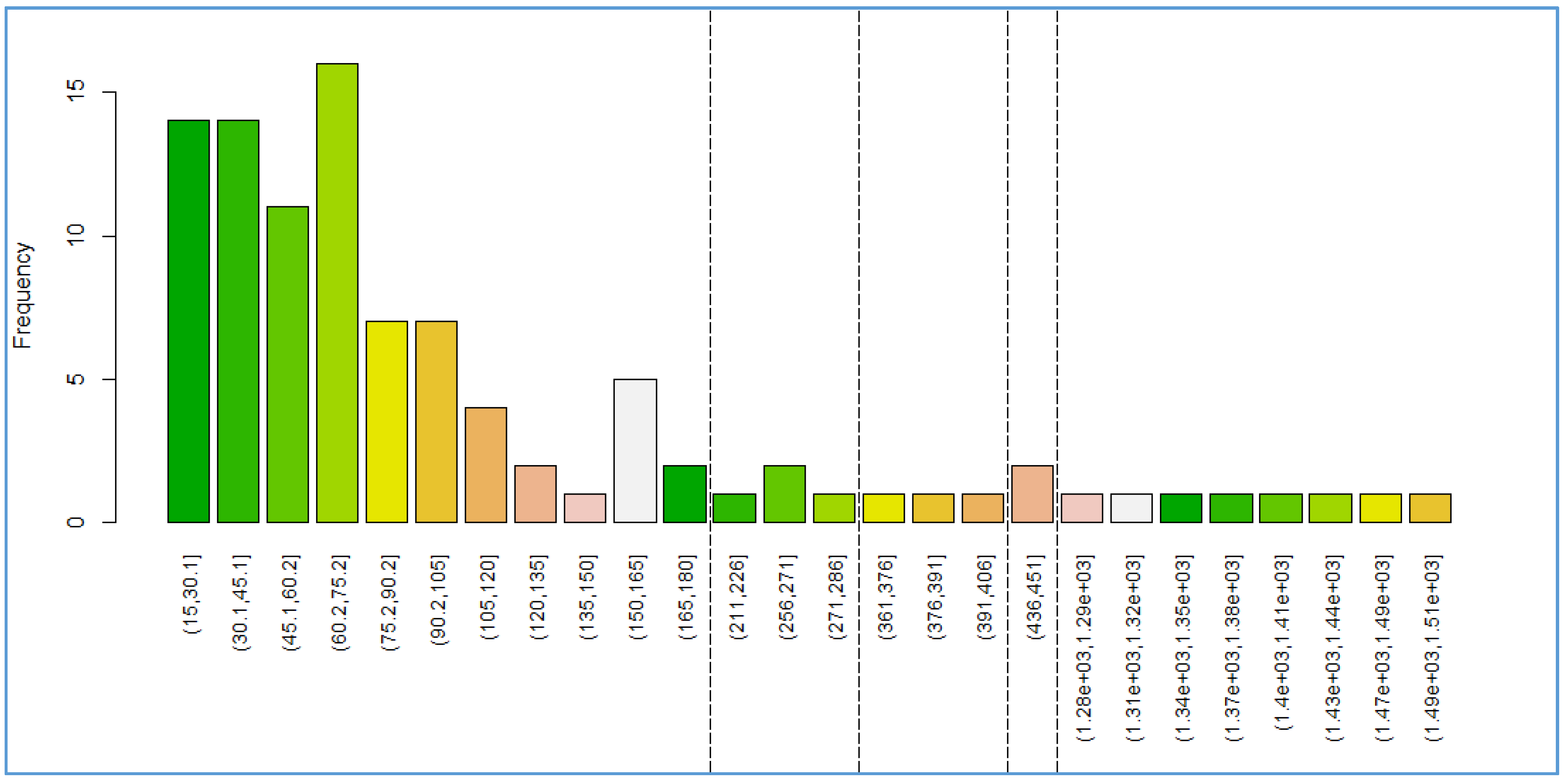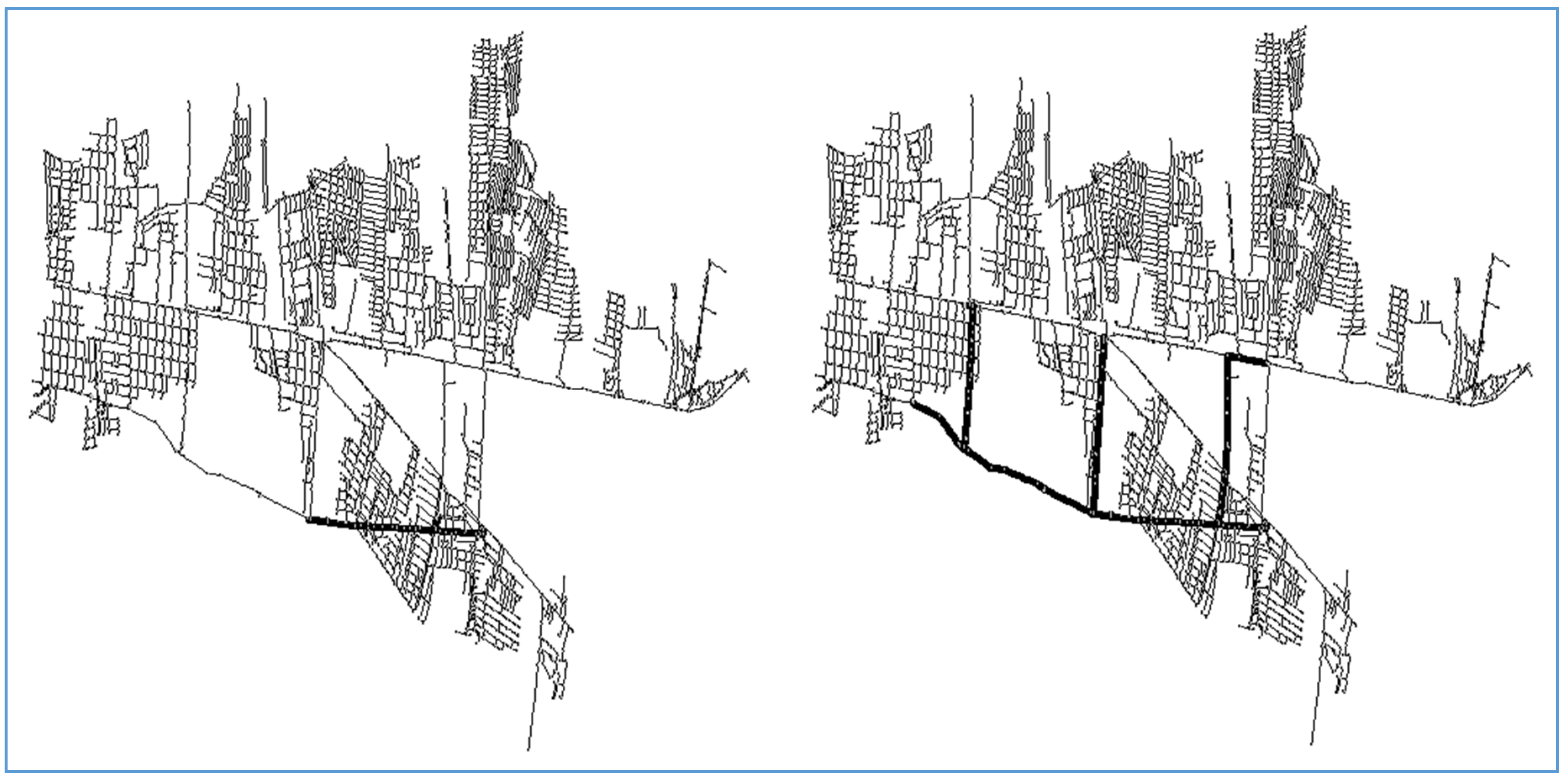Figure 2 is a zoom-in of the remaining 3% of the pipes in Figure 1. The vertical dotted lines indicate discontinuity in the ranges of ASPV*; for example, the first vertical line from the left to the right separates the ranges 165–180 and 211–226. As can be seen, the last value of the first range is lower than the first value of the second range, which indicates the presence of pipes of different classes. This type of discontinuity can be used as a criterion to define several scopes for the trunk network. For example, in the left plot in Figure 3, the trunk network selection includes all of the pipes with ASPV* above the range 211–226, whereas the one to the right includes pipes with ASPV* values above 15.

Once the trunk network is selected, it is uncoupled from the distribution network, and this last one is treated as a social network graph. Of note is that social network graphs are specific versions of graphs, where there are no centroids, and all of the nodes have the same level of importance. The community detection algorithms based the social network theory aim at revealing network modules based on a modularity index proposed by [17]. One of these algorithms corresponds to the so-called Louvain method. This is a multilevel algorithm, which works with a “bottom-up” approximation. Initially, each node is assigned to its own community. Iteratively, the algorithm builds up neighbor’s communities, with the aim of increasing the modularity index. In the next step and at a higher level, a new network of aggregated communities is formed. Then, the process is repeated until there is no more gain in the modularity index. The algorithm is classified as extremely fast and able to deal with networks of up to 10⁹ edges in a reasonable time, with ordinary computing resources [18]. It is important to note that, although the algorithm always finds a partition with maximized modularity, the result of the method is not only one partition, but a hierarchy of partitions, from which any particular partition may be selected. Let us note that the partition of maximum modularity can generate extremely small communities, whose implementation could be economically unfeasible. This is the reason why we propose a recursive merging process (see the pseudo-code below) to ensure that all of the sectors comply with a series of pre-established constraints.

In the next pseudo-code, we use the following notation:

Index m represents a pipe; IN_m represents the initial node of pipe m; FN_m is the final node of pipe m; C stands for community; and L refers to the characteristic used as a criterion.

Pseudo-Code:

All of the pipes separating communities are selected and are input into the Set of Candidate Pipes (SCP):

Input: Communities with a maximized modularity index.

1.

Given m, if IN_m ∈ C_i and EN_m ∈ C_j → m ∈ SCP.

From the SCP, a subset scp_i from which their corresponding communities do not exceed a preset constraint for a given feature is extracted.

2.

From scp_i ⊈ SCP, in which for every m, L_i and L_i < L_max.

For every m, if L_i + L_j < L_max → i + j = {i, j}.

3.

Steps 1–2 are repeated until there are no more pipes entering into the scp_i.

Output: Sectors satisfying a series of constraints.

It is also important to set a lower limit for the characteristic used to define the size of the sectors. Therefore, if at the end of the process there are some sectors with a value lower than the limit, they are declared as minisectors (no valves or CUs). This only applies in the case of minisectors that cannot be merged with larger sectors. In the case that a minisector shares at least one connection with a sector that has reached its maximum feature value, the maximum limit is slightly relaxed to allow their fusion. For example, if the characteristic that is used as a criterion is the sector pipe length (e.g., 30 km maximum constraint), the maximum final length that a given sector eventually will have will equal that maximum length (30 km) plus a value that is smaller than the minimum value of the sector pipe length (e.g., 4 km); in other words, a value between 30 km and 34 km may be accepted.

Finally, the trunk network is re-coupled with the distribution network, and the pipes connecting each sector with the trunk are included in a new set of candidate pipes. Each pipe in this set can be defined either as a boundary valve or as a sector entrance.

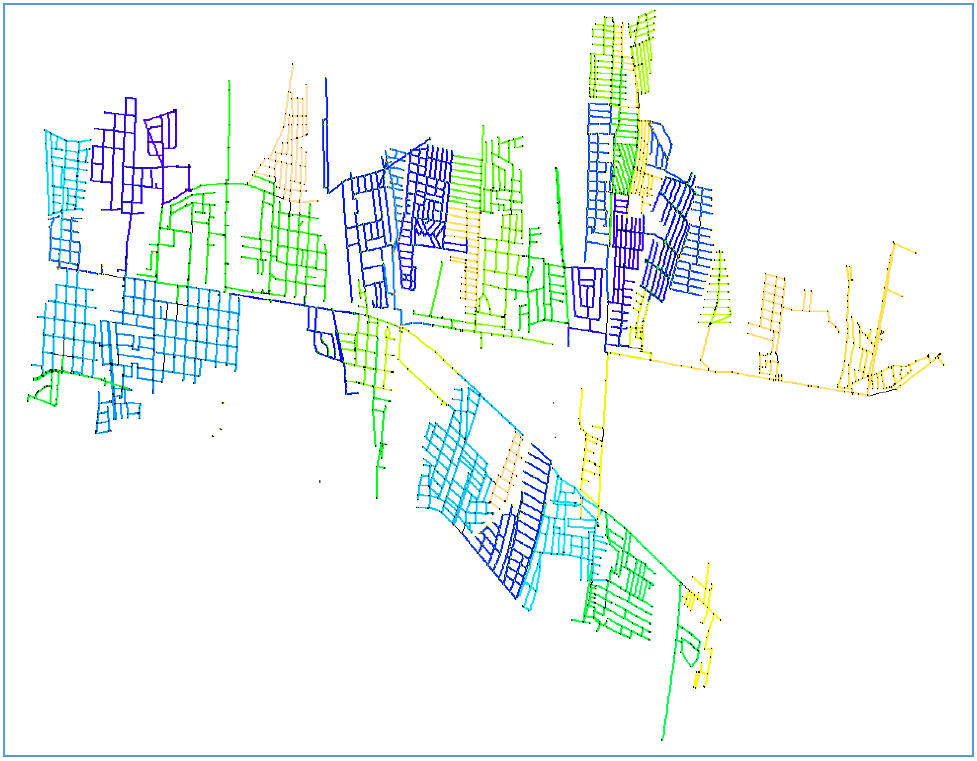
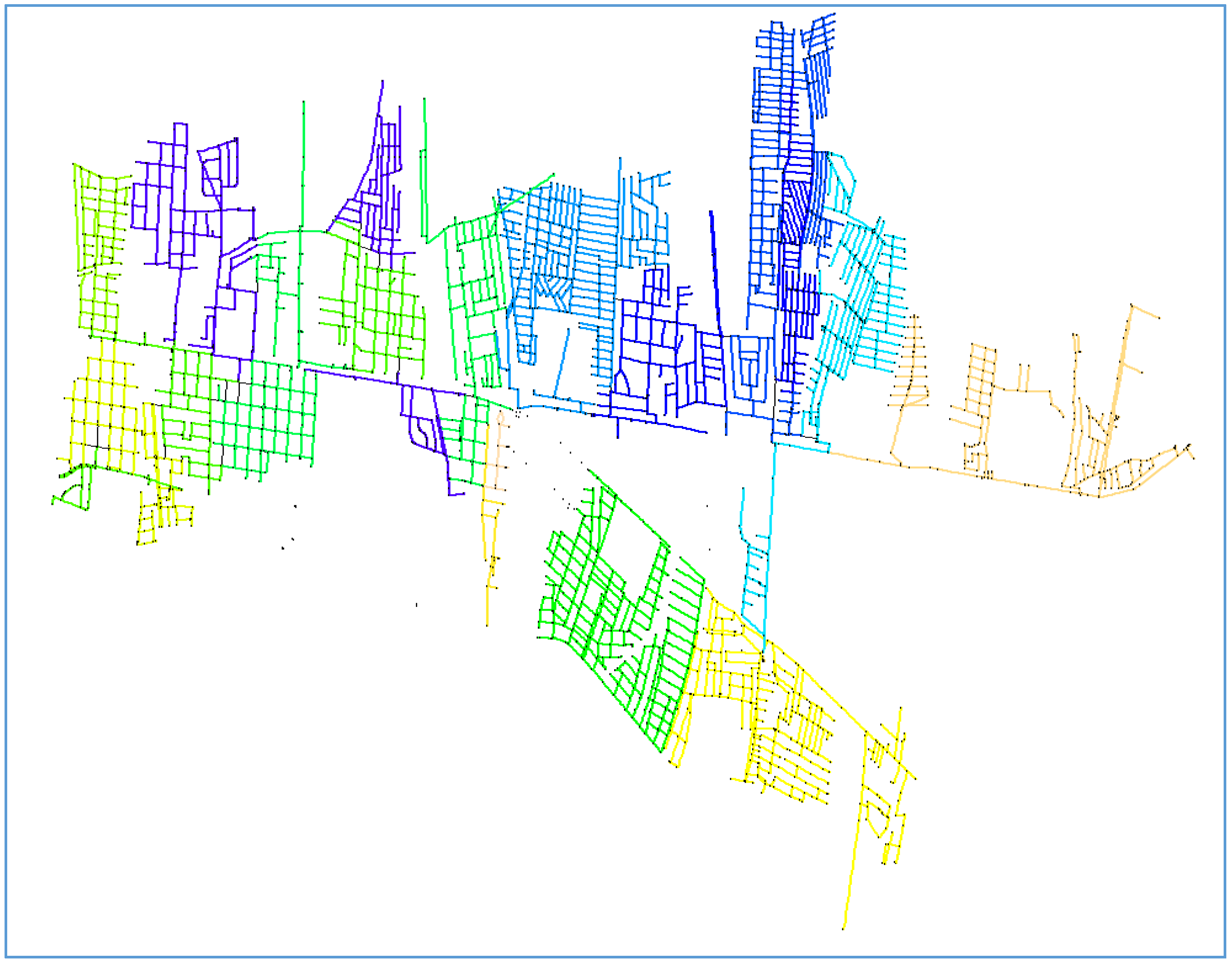
Figure 4 and Figure 5 depict the output of the merging process over the partition with the greatest modularity index for the case study in this paper. In the first case, the maximum allowed elevation difference was set at 20 m, while for the second case, it was set at 40 m. Of note is that in the first partition (Figure 4), there are many small sectors that in the second partition are merged into bigger sectors (Figure 5).

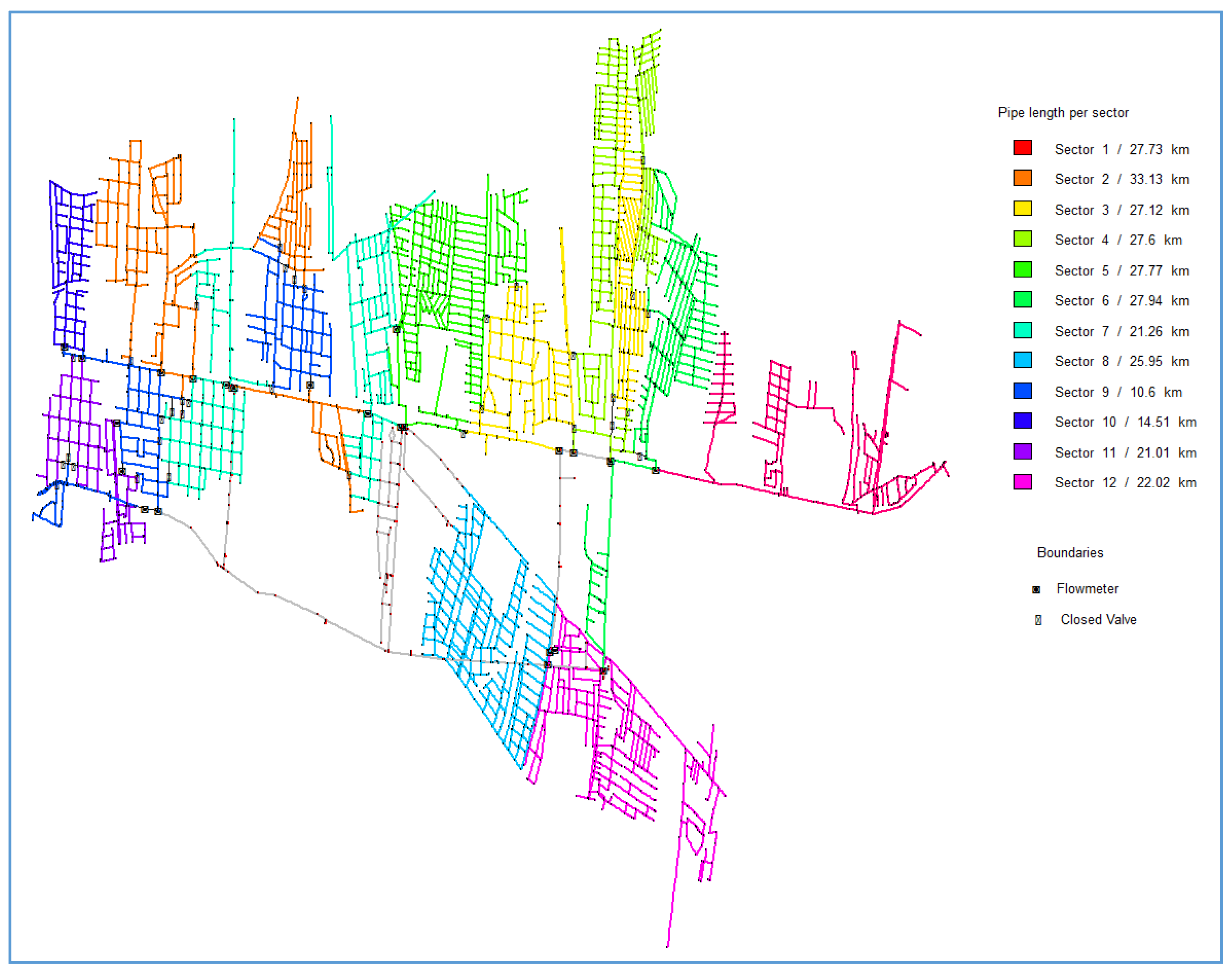
Finally, Figure 6 depicts the layout after reincorporating the trunk network. The final configuration has 12 sectors with pipe lengths between 4 and 34 km.

2.2. Optimization of the Arrangement CUs/Boundary Valves

2.2.1. Short Run Economic Leakage Level

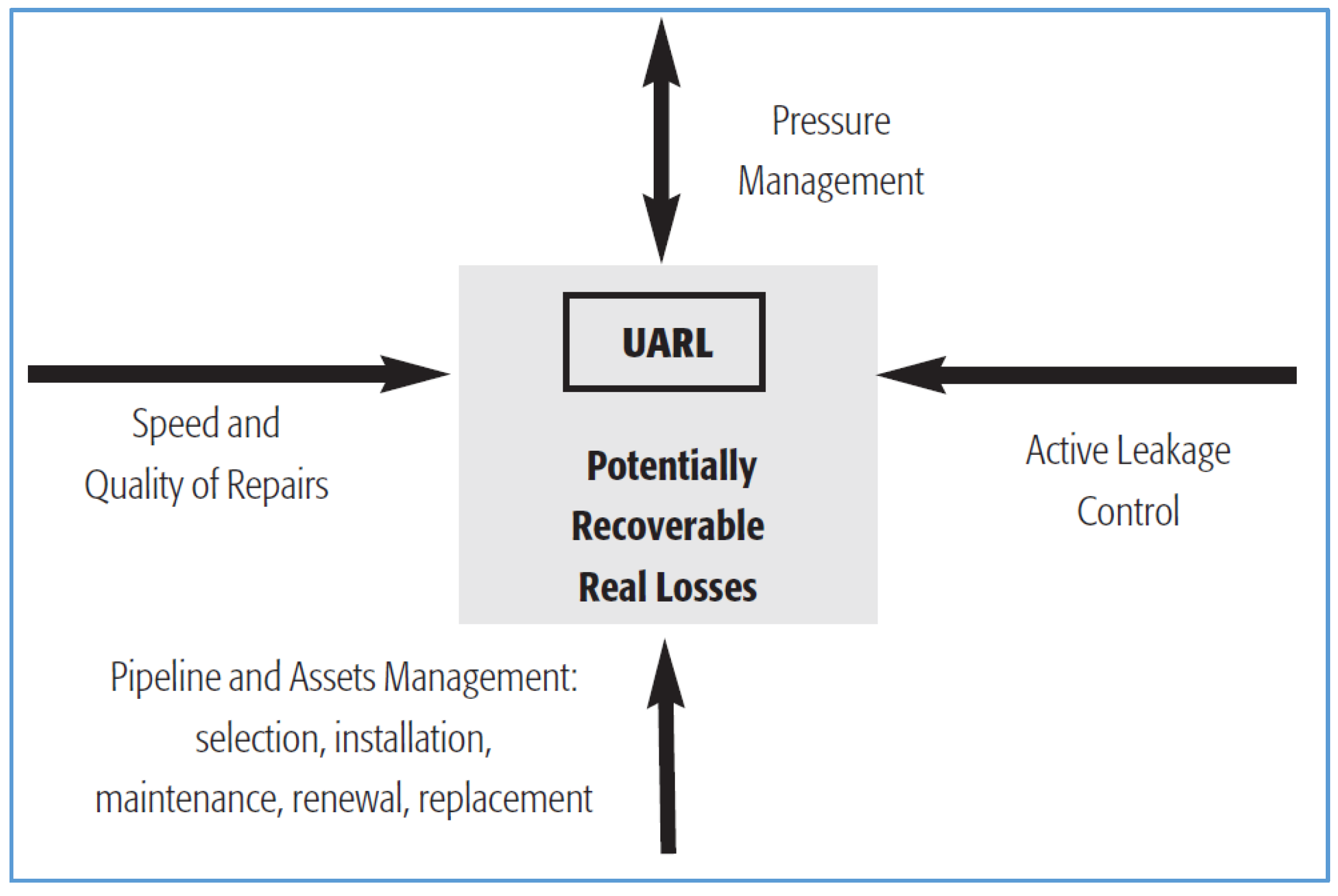
Figure 7 is broadly used to describe how real losses are structured in WSNs. It describes the way the management of real losses is conducted with four components: (1) speed and quality of repairs; (2) pressure management; (3) active leakage control; and (4) pipeline replacement. Between the Unavoidable Leakage Level (UARL) (background leakage) and the total leakage volume, there is an economic management level, which corresponds to the level where the cost of a new repair exceeds the payback.

More than a decade ago, Fantozzi and Lambert [20] proposed a method to estimate the short run economical leakage level (SRELL) based on a combination of BABE (Burst And Background Estimates)concepts, proposed by the United Kingdom National Leak Initiative [16,21] and the FAVAD (Fixed And Variable Area Discharge) theory [22]. A very important result derived from this estimate is the NRELL (Non-Reported Economical Leakage Level), which corresponds to the volume of unreported leakage that is feasible within a certain period of time.

According to the FAVAD theory (Equation (1)), the variation in the flow running through a crack in a pipe depends on the variation of the pressure in the pipe powered to N1, an exponent that is related to the characteristic of the space (rigid pipe or flexible pipe) where the leak occurs.

$$\frac{Q^1}{Q^0}={\left(\frac{P^1}{P^0}\right)}^{N1}$$

(1)

here, Q indicates leakage flow before and after some pressure variation P.

The method to estimate the SRELL starts by making a division of the leakage flow according to the BABE concept, as shown in Figure 8. In the same figure, it can be seen that, starting at time zero, background leakage remains constant over time; reported leaks (bursts) occur and are repaired (vertical bars); meanwhile, unreported leaks gradually increase until they reach a point where their cost equals the cost of inspecting the entire network. The slope of this increase is known as the Rate of Rise (RR). The average of these three components corresponds to SRELL, and it is represented by the dotted (horizontal) line in the same figure.

Of note is that reported leaks have a component-cost associated withthe flow that is lost through them and a component-cost associated withthe pipe repair. The longer the period of detection and repair, the higher the cost associated with the flow, while the component associated with the repair remains unchanged.

The method to assess the SRELL includes Equation (2) to calculate the Optimal Frequency of Inspection (OFI) of the entire WSN, based on three components: CI (Cost of Inspection) ($), CW (variable Cost of Water) ($/m³) and RR (Rate of Rise) (m³/day/year).

The RR should be evaluated by comparing the minimum night flow just before repairing all reported and unreported leaks and at least one year later. The variation of minimum night flow expressed in m³/day is then divided by the amount of years in which the evaluation was conducted, thus obtaining a value expressed in m³/day/year:

$$OFI \left(\text{months}\right)=\sqrt{\frac{0.789\times CI}{CW\times RR}}$$

(2)

From the result obtained by Equation (2), it is possible to calculate the PI (annual Percentage of Inspection),

$$PI\left(\%/\text{year}\right)=100\times 12/OFI$$

(3)

Additionally, from here, it is possible to calculate the budget that should be available every year for that purpose or ABI (Annual Budget of Inspection):

$$ABI (\$/\text{year})=PI\times CI$$

(4)

By dividing the ABI by the CW, the NRELL is obtained:

$$NRELL \left({\mathrm{m}}^3/\text{year}\right)=ABI/CW$$

(5)

The previously presented calculation can be used to predict the benefits of pressure management in a WSN. Following the principle of the FAVAD theory, by reducing the pressure in a WSN, it is expected to reduce the background, reported and unreported leaks, as shown in Figure 9. Furthermore, in the same figure, it can be seen that a pressure reduction translates into a decrease of the RR, a reduction of the time required to perform a complete inspection (which implies a reduction of the PI) and, therefore, a reduction of the ABI. The consequence of all of this is a reduction of both the SRELL and the NRELL.

2.2.2. Effect of Pressure Reduction over Burst Frequency and Domestic Consumption

In 2006, Thornton and Lambert [24] put in place the approach currently used to address the prediction of burst reduction. This approach is based on data (the relationship between pressure variation and burst reduction) from 112 WSNs in 10 different countries. The idea behind this approach is to multiply either the maximum, medium or minimum pressure variation by three constants (1.4, 2.8 or 0.7), respectively, in order to obtain a burst frequency reduction factor. With this factor, it is possible to estimate the reduction in burst frequency, as shown in Equation (6),

$$r^{\prime }=r\times BRF$$

(6)

where r′ represents the amount of bursts after reducing the pressure, r is the initial frequency of bursts and BRF stands for Burst frequency Reduction Factor.

Domestic consumption is also susceptible to pressure variations. This variation is represented by a slight modification of the FAVAD Equation (7). Now, the flow terms refer to domestic consumption (internal or external), and the exponent N1 has been replaced by a new exponent N3. For external domestic consumption, a value of N3 around 0.5 is usually employed, while for internal consumption, a value 0.1 is suitable, unless the majority of the households count on a water deposit, in which Case 0 would be more appropriate.

$$\frac{Q^o}{Q^1}={\left(\frac{P^o}{P^1}\right)}^{N3}$$

(7)

here, Q is the domestic consumption (internal and external) before and after pressure variation P.

2.2.3. Leakage Management by Means of Sectorization

From all of the above, it can be concluded that a reduction in pressure translates into economic benefits due to a reduction of:

• Background leakage;
• Reported leaks;
• Detectable unreported leaks;
• Number (frequency) of bursts;
• Domestic (internal and external) consumption.

Depending on the sectorization layout, the energy consumption may locally increase or decrease. If the increase in head loss generated by the sectorization is not excessive, the energy consumption is expected to decrease due to the reduction on leakage flow.

To reduce pressure in a WSN, the use of pressure-reducing valves is the option most broadly employed. In general terms, sectorization is not intended to reduce pressure, but to improve leakage management. However, when a WSN is sectorized, there is an unavoidable impact over pressure. This applies only in the case that boundary pipes are closed. If all sectors are delimited with flowmeters, no variations of pressure are expected. The idea herein proposed is to estimate the profit generated by sectorizing a WSN as a result of both reducing pressure and improving monitoring. To do so: (1) the FAVAD equation is used to calculate the reduction of leakage flow (background and reported leaks), domestic consumption and the NRELL; then, (2) the flow associated with reported leaks and NRELL is distributed among the sectors, based on technical criteria from the network operator; (3) depending on the pipe length and the number of entries in each sector, a percentage of leakage events’ detection (immediate detection and repair) is estimated; and (4) the value of reported leakage flow and NRELL are updated.

All of the benefits are summed in order to obtain the annual gross profit. From the result, three values are subtracted: a penalty cost associated with the nodes that fail to meet the requirements in terms of minimum pressure, a percentage of the total investment and an annual maintenance cost. Regarding the second cost, the gross profit is calculated on an annual basis; thus, the investment cost is multiplied by an amortization factor (Equation 8), in order to know the percentage of the investment that has to be covered every year. Finally, the maintenance cost is defined as a percentage of the latter.

$$AF=\frac{{\left(1+r\right)}^T\times r}{{\left(1+r\right)}^T-r}.$$

(8)

here, AF stands for amortization factor, r is the discount rate in % and T is the life span of the equipment (in this case, flowmeters and boundary valves).

To calculate the cost of energy, the hourly consumption (kWh) is multiplied by the price of energy ($/kWh) at the respective time. The daily value is converted to an annual basis and added to the gross profit; although, as explained below, it can also be added to the cost, depending on the final scheme of sectorization.

Figure 10 depicts how the benefits obtained by reducing physical losses by means of sectorization and the respective investment are related. The y axis represents the economic benefits and cost of investments; the two lines parallel to the x axis represent the total amount of candidate pipes that are set as CU or as boundary valves. It can be seen that the curves labeled as CU and boundary valves follow opposite directions, given the fact that if a pipe is not set as a CU, it is set as a boundary valve. The x axis represents the pressure reduction generated when some of the boundary valves are shutoff. Such a pressure reduction cannot exceed the supply quality standard. As the pressure is reduced, the benefits, in terms of leakage reduction, increase, as well as the cost of boundary valves. Since the establishment of sectors allows rapid detection/repairing of leakages (when they occur), the curve of savings goes beyond the benefits obtained through pressure reduction. Finally, the top line corresponds to the annual net profit (annual gross profit-annual expenditure).

2.2.4. Objective Function

In a WSN of hundreds of kilometers of pipe extension, the number of possible combinations CUs/boundary valves can be significantly large. The more CUs a given sector has, the lower is the negative impact over the pressure in its nodes, but the lower is the likelihood to detect leakage events in a short period of time.

Equation (9) shows the objective function to be maximized, followed by the constraints.

$$\begin{array}{c}\text{Max}f\left(x\right)=A+B+C+D+E+F+G\pm H-A^{\prime }-B^{\prime }-C^{\prime }\\ \text{Subject to} \Delta I_r<\Delta {I_r}^{rmax}; P_{min}<{P_{min}}^{req}; 0<\mathrm{A}+\mathrm{B}<{\left(A+B\right)}^{max}\end{array}$$

(9)

• A: savings from the reduction of background leakage (volume) ($/year);
• B: savings from the reduction of reported leaks (volume) ($/year);
• C: savings from the reduction of the number of pipes to repair (reported bursts) ($/year);
• D: savings from the reduction of the number of pipes to repair (unreported bursts) ($/year);
• E: savings from the reduction of domestic consumption (volume) ($/year);
• F: savings from the reduction of the external domestic consumption (volume) ($/year);
• G: savings from the reduction of unreported leaks (volume) ($/year);
• H: savings/expenses from decreasing/increasing energy consumption ($/year);
• A′: amortized cost of valves and CUs ($/year);
• B′: compensation cost for pressure deficit ($/year);
• C′: maintenance cost of valves and CUs ($/year);
• ΔI_r and ΔI_r^req: variation in the resilience index and maximum variation allowed;
• P_min and P_min^req: minimum pressure and minimum pressure required;
• A + B and (A + B)^max: budget for the purchase of boundary valves and CUs and the budget threshold.

Background leakages indicated by term A correspond to a leakage that is undetectable by the available technology and that can only be diminished by reducing the pressure. Reported leakages, indicated by B, are leakages that are visually detectable; C and D indicate repairing of pipe cracks for either leakages that are visually detectable or leakages that are not visually detectable, but that might be localized in a leakage detection campaign. E and F indicate the water consumption inside and outside the households(i.e., garden watering), respectively; the term G indicates leakages that can be detectable (localized) in a leakage detection campaign; H indicates the energy consumptionthrough pumping; A′ indicates the yearly cost (amortized cost) of investment for the purchase of boundary valves and CUs; B′ indicates the cost of compensation for the nodes that cannot meet the duty pressure, which is estimated by multiplying the total demand of the critical nodes by the cost of supplying one cubic meter of water by means of a cistern.

The resilience index used here corresponds to the index proposed by Todini [25], which is calculated by subtracting from 1 the fraction that represents the current head loss over the total head loss required to ensure that all of the nodes meet a certain pressure threshold.

It is important to note the complexity of the objective function, especially if it is compared to theobjective functions used in previous research work. In fact, such an approach has two maindrawbacks. The first one is related to larger calculation times. Nevertheless, as previously explained, the reduction of pressure by means of sectorization brings very important benefits that should be taken into consideration in order to make the optimization more realistic. One way to solve the calculation time problem could be the grouping of some of the benefits (parameter) into one single parameter; however, this would require new research in order to know how they are interrelated, which at this moment is not really clear and, in fact, is one of the topics on which the authors are currently working. The second drawback is related to the information itself, since it is not easily obtained and, on the contrary, requires a big effort from the water authority.

2.2.5. Monte Carlo Simulations to Deal with Uncertainties in the Optimization Process

The ability to detect and locate new leakage events will depend on two characteristics of each sector: the sector pipe length and the number of CUs; it also depends on the technical capacity of the water operator. The probability of detecting and locating a new leakage event is inversely proportional to its size and the number of CUs. Due to the lack of a mathematical formulation to describe this probability, this information should be estimated by the technical staff of the water utility based on their experience.

Values in

Table 1. Percentages of leakage event detection as a function of the sector size and CUs.

Sector Size (Pipe Length-km)	Amount of CUs		Detection Percentage
0–10	0	1	30%
	2	3	20%
	4	5	10%
	6	7	5%
	8	9	5%

can be set as single values (fixed values) and then be used in a classical optimization model. In other words, a single leakage flow volume that is controlled due to the sectorization implementation is defined. However, the prediction of a percentage of detection has a high degree of uncertainty. To deal with this, we propose to represent such a percentage as a range of probabilities. This range can be defined by probability curves (or by an equation describing the probability density). In this regard, there is a broad range of distribution curves that can be used; however, in this work, we select a “triangular”distribution, based on the fact that only the minimum and maximum expected values and a trend are required for its construction. This type of curve, despite the lack of precision, has the advantage of being useful when data are missing (due to the high cost of collection). However, it is possible to estimate the relationship between them.

Leakage flows are expected to be differently distributed among the sectors (sectors located in older and/or with less maintenance areas are expected to have a higher frequency of leakage than those located in newer and/or better managed areas).The allocation of the expected leakage rate in each sector must be carried out by the technical staff of the water utility based on their experience.

Once the detection probability curve of each sector is established, the optimization process is initialized; however, differently from a classical optimization model, for each iteration that generates a feasible solution, an MCS is carried out. Accordingly, probabilistic values are randomly sampled from the predefined distribution curves. Then, the average of each sampling is calculated and included in the objective function. The solutions in which the simulation result meets the established constraints are marked as valid and used as feedback to generate new solutions, while the solutions outside the feasible region are discarded.

Figure 11 depicts the whole methodology. The first column (left) shows the sector definition algorithm; while the section to the right shows the process to optimize the arrangement entrances/boundary valves. In this part, for every iteration, a solution vector is generated by the GA and imputed in the simulation. Then, the constraints are reviewed. If the solution meets the constraints, an MCS is conducted; otherwise, the solution is discarded. It is important to note that the results of the MCS depend on the solution generated by the GA and on the event detection probability curve. Once the MCS is completed, the constraints are revised; if they are met, the objective cells are updated; otherwise, the results of the MCS are discarded.

The community detection process is carried out with the Igraph package [26] implemented in R, and the optimization of CUs and boundary valves is conducted with the RiskOptimizer^® tool [27].

3. Results and Discussion

Some of the obtained results have already been shown as examples in the development of the materials and methods in Section 2. Specifically, Figure 1, Figure 2, Figure 3, Figure 4, Figure 5 and Figure 6 exhibit some of the results obtained.

Now, we present the results corresponding to the optimization process to identify an optimal distribution of CUs and boundary valves in the network.

To calculate the amortization factor, (see

Table 2. Calculation of the amortization factors used in the example of the implementation.

Sectorization Equipment	Life Span (year)	Interest Rate	Amortization Factor
CUs	10	0.2	0.21
Boundary valves	5	0.2	0.22

) the annual interest rate was set at 20.0% for both CUs and boundary valves. The life span of CUs was set at 10 years, and the life span of boundary valves was set at five years. The cost of maintenance was set to a value equivalent to 50.0% of the percentage of the investment that has to be covered every year. These values do not correspond to any real standards; they were manually selected for example purposes. The authors tried to get this information from the water authority of Managua City, but unfortunately, it was not possible.

Figure 12 depicts the final sectorization layout (with CUs and boundary valves).

This discussion is centered on the real profit derived from the implementation of the proposed approach and the discussion about the differences with other sectorizations not considering some of the benefits derived from sectorization, which we have integratedin our approach.

The CUs and boundary valve optimization process produced as a result 23 CUs and 37 boundary valves. As can be seen in

Table 3. The Resilience Index (Ir) comparison between the original network and the sectorized network.

Control Parameter	Initial	Final
Ir	0.7	0.5

, the resilience index did not experience significant reduction.

Table 4. Costs/benefits balance obtained for the example network.

Benefits Section
Control Parameters	Initial (m3/year)	After Optimization (m3/year)	Reduction before MCS (m3/year)	Reduction after MCS (m3/year)	Saves ($/year)
Background leakages	151,587.3	110,102.3	41,245.0	NA	32,996.0
Detectable leakages	145,000.0	140,000	5000.0	9418.0	7534.0
Internal demand	155,000.0	150,195.0	4805.0	NA	3844.0
External demand	15,500.0	13,253.0	2248.0	NA	1798.0
Control parameters	Initial ($/year)	After optimization ($/year)	Reduction before MCS ($/year)	Reduction after MCS ($/year)	Saves ($/year)
Inspection costs	21,716.0	8966.8	12,749.5	181,238.0	16,238.0
Energy	15,354.8	11,354.0	4000.8	NA	4000.8
Control parameters	Initial yearly break/year rate	yearly break/year rate after optimization	Reduction of yearly break/year rate after	Reduction after MCS
Reported bursts	333	79	254	NA	15,800.5
Unreported bursts	200	47	153	NA	10,690.9
Total benefit ($/year)					92,901.7
Costs Section
Investments and expenditure	Total ($)		After discount ($/year)
CUs	234,355.9		49,214.6		49,214.6
Boundary valves	59,651.6		12,526.8		12,526.8
Deficit compensation	5587.3		-		5587.3
Total Investment + Operation Costs ($/year)					67,328.8
Net profit ($/year)					25,572.9

and Figure 13 show the annual net profit (savings minus expenditures) corresponding to 25,572 $/year.

It is interesting to note that the sum of the new benefits that we are taking into consideration (detectable leakages, internal and external demand, inspection cost and benefits in term of repairing) are significantly greater than the benefits associated only with the reduction of background leakages. Globally, the total savings related to the new benefits (59,908.0 $/year) is 44.9% higher than the savings generated by the reduction of background leakages (32,996.0 $/year). From another perspective, the advantage of the proposed approach is evidenced by the fact that background leakages’ reduction represents 35.5% of the total gross benefit, while the new benefits represent 64.4% of the latter. In fact, if the cost of investment + expenditure is compared only to the savings in background leakages and energy, the project would be unfeasible (see Figure 13). Furthermore, if only the new benefits are considered, the project would be unfeasible; nevertheless, it is important to consider two aspects. Firstly, the deficit in the second case would be significantly smaller than in the first case, and secondly, the estimation of the new benefits is more complex than the evaluation of background leakages and energy; therefore, it is very unlikely to have them without having the values/costs of background leakages and energy.

It is also interesting to note that the reduction in the detectable leakages is divided into two parts: the first part is related to the reduction of the pressure, which represents 82.9% of the original volume, and the second part is related to the enhancement of the capacity to detect leakage events, representing only 6.4% of the original volume. Evidently, the values of the second part can dramatically change depending on the technical capacity of the water operator.

As mentioned in the Introduction, this is the first research that encompasses the analysis of benefits beyond the reduction of the current level of background leakage. To our knowledge, there are no similar research works in the literature, and thus, it can be affirmed that it has a great level of novelty. Despite the interesting results that can be obtained when implementing this methodology, there are some aspects that must be further tackled. One of these aspects is the use of MCS during the optimization. From the outset, it would be very important to define a methodological procedure to distribute the bulk of reported and unreported (detectable) leakages over the sectors and the percentages of detection given the characteristics of each sector. Moreover, it would be interesting to study the effect of different types of probability distribution curves in order to simulate the probability of leakage events’ detection.

4. Conclusions

In the present paper, we address a topic of major and current relevance: the analysis of the benefits, in economic terms, generated by the implementation of a sectorization project in a WSN. A methodological development of leakage analysis, based on some concepts proposed by the IWA, is implemented. This development allows considering the benefits of sectorization, beyond the savings generated only by reducing existing leakages, which is the economic criterion most broadly considered in previous sectorization methodologies. This work integrates new concepts in the sectorization research field, such as social network theory community detection algorithms and Monte Carlo simulation. The first concept detects sectors based on the network topology, which is very important in networks that rely on a trunk network. The communities’ recursive merging process herein proposed allows tailoring the results of the multilevel communities’ detection algorithm to the problem of sectorization, thus obtaining sectors with a series of preset constraints. Additionally, Monte Carlo simulation allows integrating within the optimization the CU and boundary valves’ arrangement and the uncertainties in the prediction of the occurrence and detection of future leakage events. We hope that this research will provide new guidelines for researchers and professionals involved in the field of WSN sectorization.