Article

Multi-Site Validation of the SWAT Model on the Bani Catchment: Model Performance and Predictive Uncertainty

1
Graduate Research Program (GRP) Climate Change and Water Resources, West African Science Service Centre on Climate Change and Adapted Land Use (WASCAL), University of Abomey-Calavi, 01 BP 526 Cotonou, Benin
2
Centre Regional AGRHYMET, PB 11011 Niamey, Niger
3
Department of Aquatic Ecosystem Analysis and Management, Helmholtz Centre for Environmental Research—UFZ, Brueckstrasse 3a, 39114 Magdeburg, Germany
4
Centre de Recherche et des Technologies des Eaux (CERTE), BP 273, 8020 Soliman, Tunisia
*
Author to whom correspondence should be addressed.
Water 2016, 8(5), 178; https://doi.org/10.3390/w8050178
Submission received: 14 March 2016 / Revised: 20 April 2016 / Accepted: 21 April 2016 / Published: 30 April 2016
(This article belongs to the Special Issue Hillslope and Watershed Hydrology)

Abstract

:
The objective of this study was to assess the performance and predictive uncertainty of the Soil and Water Assessment Tool (SWAT) model on the Bani River Basin, at catchment and subcatchment levels. The SWAT model was calibrated using the Generalized Likelihood Uncertainty Estimation (GLUE) approach. Potential Evapotranspiration (PET) and biomass were considered in the verification of model outputs accuracy. Global Sensitivity Analysis (GSA) was used for identifying important model parameters. Results indicated a good performance of the global model at daily as well as monthly time steps with adequate predictive uncertainty. PET was found to be overestimated but biomass was better predicted in agricultural land and forest. Surface runoff represents the dominant process on streamflow generation in that region. Individual calibration at subcatchment scale yielded better performance than when the global parameter sets were applied. These results are very useful and provide a support to further studies on regionalization to make prediction in ungauged basins.

Graphical Abstract

1. Introduction

Water resources managers are facing challenges in many river basins across the world due to limited data availability. Anthropogenic activities add more uncertainties to this task by inducing changes to land and climate at different scales [1,2]. This situation is more pronounced in developing countries, where in many river basins no runoff data are available [3,4,5,6,7] and the existing ones are of questionable quality or, at best, short or incomplete.
The Niger River basin is not an exception to that rule. The general situation of insufficient data is exacerbated by a deterioration of measurement networks. In the 80s and 90s, for instance, hydrometric stations were reduced to a minimum and many have been abandoned (e.g., [8]). To prevent the hydrologic observing system from more degradation, the Niger Basin Authority (NBA) has set the Niger-HYCOS project, which one of its specific objectives is to improve data quality of the Niger Basin. For this purpose, the project identified and brings assistance in the installation and the management of 105 hydrometric stations shared by nine countries drained by the River, and contributes to the capacity building of national hydrological services.
In its fifth assessment report on regional aspects of climate change, the Inter-Governmental Panel on Climate Change [9] has shown that adaptation to climate change in Africa is confronted with a number of challenges among which is a significant data gap. Too many basins lack reliable data necessary to assess, in details, impacts of climate change on different components of the hydrological cycle and to develop strategies of adaptation related to each specific impact. Thus, it is germane to predict hydrological variables in ungauged basins for building high adaptive capacity by improving: (i) water resources knowledge, planning, and management; (ii) identification and implementation of strategies of adaptation to climate change in the sector of water, and (iii) ecological studies for a sustainable development.
The application of rainfall-runoff models and then, transferring model parameters from gauged to ungauged catchments is a long-standing method [10] for flow prediction in ungauged basins and has been highlighted during the decade of Prediction in Ungauged Basins (PUB) launched in 2003 by the International Association of Hydrological Sciences (IAHS) and concluded by the PUB Symposium held in 2012. This is the framework of the present study, in which the Soil and Water Assessment Tool (SWAT) model was calibrated on the Bani catchment (Niger River basin) and the most sensitive model parameters were estimated.
Many studies have successfully applied the SWAT model in West Africa, on different river basins. Examples include, among others: calibration of the SWAT model on the Niger basin [11,12,13,14,15,16], the Volta basin [12,13,14,15,17,18,19] and the Oueme catchment in Benin [15,20,21,22]. However there are few published papers on the application of the SWAT model on the Bani catchment. For instance, Schuol and Abbaspour [12] and Schuol et al. [14] applied the SWAT model to selected watersheds in West Africa including the Niger basin and modeled monthly values of river discharges (blue water) as well as the soil water (green water), and clearly showed the uncertainty of the model results. They developed and applied a daily weather generator algorithm [13] that uses 0.5 degree monthly weather statistics from the Climatic Research Unit (CRU) to obtain time series of daily precipitation as well as minimum and maximum temperatures for each sub-basin. These generated weather data were then used as input for model setup and the authors concluded that “discharge simulations using generated data were superior to the simulations using available measured data from local climate stations”. Reported Nash-coefficient values obtained vary largely between sub-basins and were principally presented as average intervals limiting thus, our understanding of model performance at finer spatial (subbasin) and temporal (daily) scales.
Laurent and Ruelland [23] successfully calibrated SWAT on the Bani catchment using daily measured climate data. They interpolated precipitation data on a regular grid by the Inverse Distance Weighted (IDW) method, which has proven to yield better results than kriging, Thiessen and spline methods, especially when a hydrological model is used [24]. To show the model performance, Laurent and Ruelland [23] reported both discharge and biomass calibration results on an average annual basis, but did not assess model calibration uncertainty. Moreover, both above-mentioned studies performed interpolation of input data out of the model framework to obtain a time series of daily weather data for each sub-basin. However, the results of interpolation methods are strongly influenced by the density and spatial distribution of the measurement stations used in the interpolation [25]. Such a density of data is not always available in developing countries.
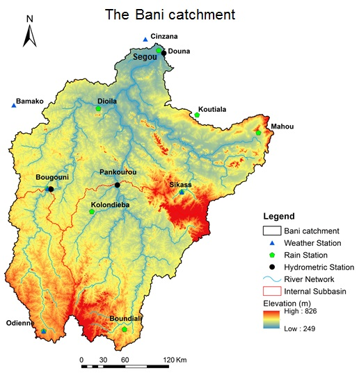
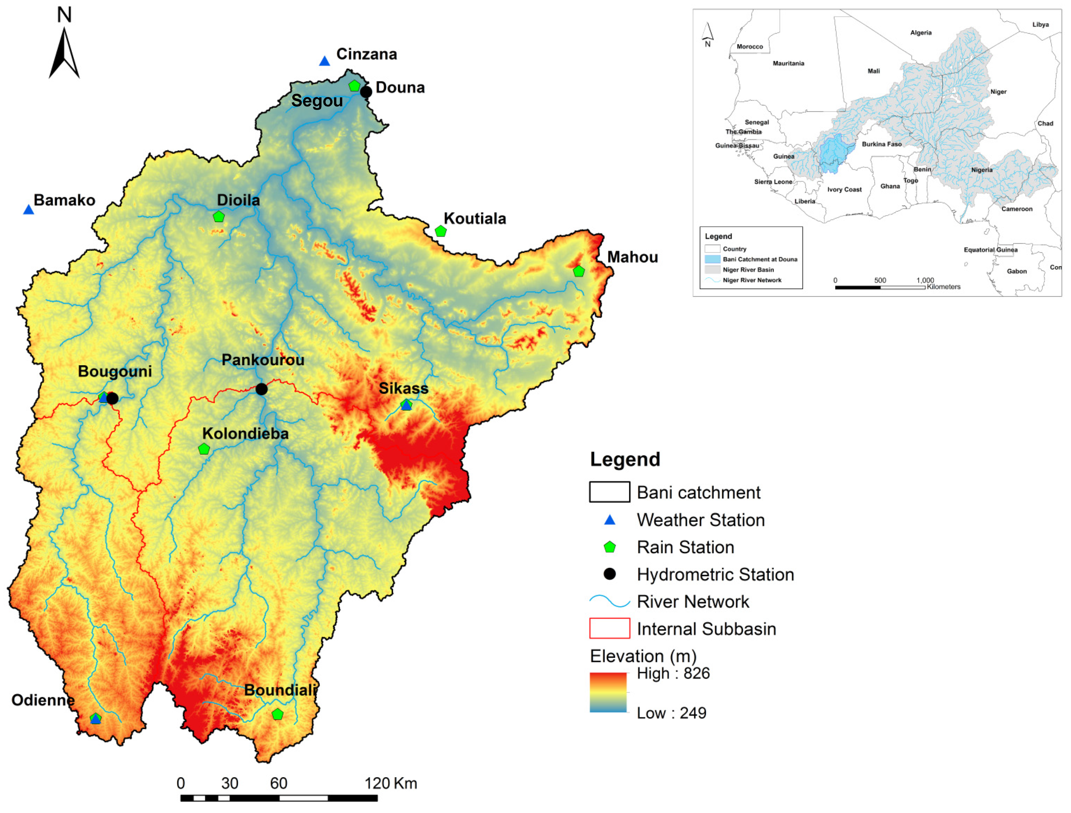
Against this background, the objective of this study was to assess the performance of the SWAT model and its predictive uncertainty on the Bani at catchment and subcatchment levels. More specifically, this meant to: (i) set up a hydrological model for the Bani catchment using the SWAT program; (ii) calibrate the model at the catchment outlet at daily and monthly time steps and assess the predictive performance and uncertainty; (iii) evaluate the spatial performance of the watershed-wide model within the catchment by validating it at two internal stations; and (iv) calibrate the model at the sub-catchments separately and provide a comparative assessment of the model performance at different spatial scales.
The originality of this study was the daily performance of the SWAT model at the whole catchment outlet and at two internal stations. Another important output of this paper was the involvement of evapotranspiration (the most important component of the water balance after rainfall especially under warm climate) in the verification of model outputs reasonability, a particular attention that has not been considered by any previous study in the region. In addition, we used in the current work point rain gauge data (as per SWAT’s standard procedure) opposed to areal precipitation as used in previous studies [12,13,14,15,24,26,27] on the same basin in order to maintain the real data condition (limited in time and space) to the extent possible.

2. Material and Methods

2.1. The Study Area

The Bani is the major tributary of the Upper Niger River. Its drainage basin is principally located in Mali but spans in a lesser extent over Cote d’Ivoire and Burkina Faso and covers an area of about 100,000 km2 at Douna gauging station (Figure 1). The Bani watershed was chosen for this study, on one hand, due to its relatively high-quality data availability compared to regional situation. It thus constitutes the appropriate gauged catchment in different hydro-climatic variables. On the other hand, this watershed has not been affected by important hydraulic structures able to significantly modify its flow regime, making the hydrological modeling of that catchment more convenient.
The catchment’s topography (Figure 1) is characterized by a gentle elevation that ranges from 826 m in the South and the center-east to 249 m at the outlet in the North. According to FAO (2003) [28], major soil groups are mainly constituted by Luvisol, Acrisol, and Nitosol (Figure 2a). Based on the USGS Global Land Cover Characterization (GLCC) version 2.0 [29], agricultural land constitutes the dominant land use category followed by savannah and forest (Figure 2b). The Bani catchment is characterized by a Sudano-Sahelian climatic regime. The river flows from south to north along a high rainfall gradient. Annual precipitation varies from 1250 mm at Odienne to 615 mm at Segou (average of the period 1981–2000). The average annual discharge recorded at Douna gauging station between 1981 and 2000 was 184 m3 s−1, which is equivalent to 58 mm of surface runoff depth for an average annual precipitation of 1000 mm. The smallest runoff values were recorded during the years 1983, 1984, and 1987. Due to climate change, there was an abrupt decrease in rainfall in the period 1970–1971 and remained for two decades [27,30] with a more severe impact on water resources. A decrease of more than 60% in discharge at Douna [27,31] and lower contribution of baseflow to the annual flood [32,33] have been reported since the 70s. Concerning future climate change impacts, the Bani basin is projected to experience substantial decrease in rainfall and runoff especially in the long term behavior [27].

2.2. Model Description

SWAT is a river basin, or watershed, scale model developed to predict the impact of land management practices on water, sediment, and agricultural chemical yields in large, complex watersheds with varying soils, land use, and management conditions over long periods of time [34]. The model is semi-distributed, physically based and computationally efficient, uses readily available inputs and enables users to study long-term impacts [35]. For a detailed description of SWAT, see Soil and Water Assessment Tool input/output version 2012 [36] and the Theoretical Documentation, Version 2009 [37].
The ArcSWAT (ArcGIS extension) is a graphical user interface for the SWAT model. In the present study, the recent version, ArcSWAT2012, was used for building the hydrological model of the Bani catchment.
The hydrologic cycle simulated by SWAT is based on the water balance equation:
S W t = S W 0 + i = 1 t ( R d a y Q s u r f E a W s e e p Q g w )
where, SWt is the final soil water content (mm H2O), SW0 is the initial soil water content on day i (mm H2O), t is the time (days), Rday is the amount of precipitation on day i (mm H2O), Qsurf is the amount of surface runoff on day i (mm H2O), Ea is the amount of evapotranspiration on day i (mm H2O), Wseep is the amount of water entering the vadose zone from the soil profile on day i (mm H2O) and Qgw is the amount of groundwater exfiltration on day i (mm H2O).
SWAT divides a basin into sub-basins which are further discretized into hydrologic response units (HRUs), based on unique soil-land use-slope combinations. The subdivision of the watershed enables the model to reflect differences in evapotranspiration for various crops and soils. Runoff is predicted separately for each HRU and routed to obtain the total runoff for the watershed. This increases accuracy and gives a much better physical description of the water balance [37].
Various hydrological models exist and there is no strict guideline on the selection of the model. The SWAT model uses a modified version of the Curve Number method, which was developed in the US for specifically calculating surface runoff generation. Therefore the model is especially suitable for regions with a high share of overland flow on total runoff. Other advantages of the SWAT model are that it allows a number of different physical processes (hydrologic, sediment, pollutants) to be simulated in a watershed. It has been previously validated for several large-scale watersheds throughout different climate contexts across the globe and has performed satisfactorily even in data poor and complex catchments (e.g., [38,39]). SWAT is also very flexible in terms of using specific and appropriate soil and land use information’s of the watershed to be modeled by adding them to its database. However in this context, it is worth using a low cost or free model, which West African National Hydrological services could afford due to economic constraints.

2.3. Input Data and Databases

The SWAT model for the Bani was constructed using weather data and globally and freely available spatial information described in Table 1. Daily precipitation data from 11 rain gauges as well as daily maximum and minimum temperature from five weather stations located mainly on the catchment were used as input. The location and spatial distribution of input precipitation and temperature stations are represented in Figure 1.
It is worth noting the weak spatial density of the measuring network that is characterized by a rain gauge for more than 9000 km2. Precipitation data are complete at the majority of the sites except for a few numbers of them, where the maximum missing data percentage varies between 8.5% and 100% in a year. Many more missing values are recorded in the temperature data. Collected climate data time series were of varying lengths. Thus, a common period of observation from 1981 to 2000 was first determined. Retained data then underwent a thorough quality control as recommended by the World Meteorological Organization (WMO) in the guide to climatological practices, third edition [40]. Three procedures were applied: (1) completeness check; (2) plausible value check; and (3) consistency check. The aim of the check is to detect erroneous data in order to correct and, if not possible, to delete it. Missing values were filled by the weather generator during the running time. For this purpose, the excel macro WGNmaker4 [41] was used to calculate weather stations statistics needed to generate representative daily climatic data.
Two different databases were used to set up the model. The SWAT database is composed by the crop database and the user soils database, both included in swat2012.mdb. They are named crop1 and soil1, respectively. Crop1 was kept default whereas soil1 was filled with soils transferred from mwswat2009.mdb (the database of the MapWindow interface for SWAT). The second database is composed by crop2 and soil2. Four land use categories define crop2: forest, savannah-bush, savannah, and steppe whereas six major soil groups are added to soil2: Acrisol, Cambisol, Gleysol, Lithosol, Luvisol ferrique, and Nitosol. Detailed description of this database can be found in [23].
For calibration purpose, we used daily river discharge data at Douna, Bougouni and Pankourou stations covering the period 1981–2000, obtained from AGRHYMET and the National Hydraulic Direction of Mali. The period 1981–1997 was kept for calibration and validation processes as it exhibits few gaps. Small existing gaps were thus filled by a simple linear interpolation.

2.4. Model Setup

The catchment was delineated and divided into sub-catchments based on the DEM. A stream network was superimposed on the DEM in order to accurately delineate the location of the streams. The threshold drainage area was kept as default and additional outlets were considered at the location of stream gauging stations to enable comparison of measured discharge with SWAT results. The whole catchment was so discretized into 28 sub-catchments, which were further subdivided into 181 HRUs based on soil, land use, and slope combinations. Further parameters have been edited through the general watershed parameters and SWAT simulation menus and are reported in Table 2. Four simulations were performed based on land use and soil databases combinations: crop1soil1, crop1soil2, crop2soil1, and crop2soil2. A Nash-Sutcliffe Efficiency (NSE) [45] was thereafter calculated at Douna by comparing measured discharges against each default simulation and the one which will yield the highest NSE value will be kept for calibration and validation processes.

2.5. Calibration and Validation Procedures

It is commonly accepted in hydrology to split the measured data either temporally or spatially for calibration and validation [36]. In addition to the split-sample method, a split-location calibration and validation approach has been performed because the global parameter set is not expected to be optimal for sub-catchments processes in view of the high heterogeneity in terms of climate, topography, soil, and land use characterizing such a large-area watershed. This approach is especially needed when prediction at data sparse sites is foreseen [46,47]. In the split-sample approach, the model was calibrated using discharge data solely measured at the catchment outlet by splitting the homogenous period mentioned in Section 2.3 into two datasets: two-thirds for calibration (1983–1992), and the other one for validation (1993–1997). To implement the split-location method, the model was calibrated at Douna and then validated at intermediate gauging stations (Bougouni and Pankourou) by turning the model on the same period (1983–1992), using the same behavioral parameter sets determined at the outlet.
Calibration was thereafter performed at Bougouni and Pankourou stations individually, and both modeling frameworks facilitated a comparative analysis of model performance and predictive uncertainty through scales. At this step, the calibration at Bougouni did not succeed within realistic range of the Curve Number (CN). Then, the daily CN calculation method was changed to Plant ET for simulation at Bougouni because soil moisture method is found to predict too much runoff in shallow soils [36]. An additional parameter (CNCOEF) was then necessary as required by the plant ET method and fixed to 0.5 in the Edit SWAT input menu.
Calibration/validation, uncertainty analysis, and sensitivity analysis were performed within the SWAT Calibration and Uncertainty Programs SWAT-CUP version 2012 [48] using Generalized Likelihood Uncertainty Estimation (GLUE) procedure [49]. GLUE is a Monte Carlo based method for model calibration and uncertainty analysis. It was constructed to partly account for non-uniqueness of model parameters. GLUE requires a large number of model runs with different combinations of parameter values chosen randomly and independently from the prior distribution in the parameter space. The prior distributions of the selected parameters are assumed to follow a uniform distribution over their respective range since the real distribution of the parameter is unknown. By comparing predicted and observed responses, each set of parameter values is assigned a likelihood value. The likelihood functions selected here is principally the NSE as it is very commonly used and included in SWAT-CUP for GLUE performance assessment. In this study, the number of model runs was set to 10,000 and the total sample of simulations were split into “behavioral” and “non-behavioral” based on a threshold value of 0.5, a minimum threshold for NSE recommended by [50] for streamflow simulation to be judged as satisfactory on a monthly time step. In that case, only simulations which yielded a NSE ≥ 0.5 are considered behavioral and kept for further analysis.
In the calibration procedure, we included 12 parameters that govern the surface runoff and baseflow processes. The real approached baseflow alpha factor (ALPHA_BF) value has been determined by applying the baseflow filter program developed by [51] and modified by [52] to streamflow data measured at the three outlets. One novelty in this study was to involve the Manning’s roughness coefficient for overland flow (OV_N) and the average slope length (SLSUBBSN) parameters that are not commonly used in calibration. The reason behind this choice was to correct the tendency of the model to delay the runoff as detected by graphical analysis. The remaining parameters were chosen based on the literature [53,54,55] and their adjusting ranges from the SWAT Input/Output version 2012 document (e.g., [56]).

2.6. Model Performance and Uncertainty Evaluation

To evaluate model performance, both statistical and graphical techniques were used as recommended by [50] based on previous published studies. The following quantitative statistics were chosen: NSE to quantify the relative magnitude of the residual variance (“noise”) compared to the measured data variance, PBIAS for water balance error, and R2 to describe the degree of collinearity between simulated and measured data, and were given for the best simulation. The NSE, R2 and PBIAS were determined using the following equations:
N S E = 1 i = 1 n ( Y i o b s Y i s i m ) 2 i = 1 n ( Y i o b s Y o b s ¯ ) 2 ,
R 2 = ( i = 1 n ( Y i o b s Y o b s ¯ ) ( Y i s i m Y s i m ¯ ) i = 1 n ( Y i o b s Y o b s ¯ ) 2 i = 1 n ( Y i s i m Y s i m ¯ ) 2 ) 2 ,
P B I A S = i = 1 n ( Y i s i m Y i o b s ) × 100 i = 1 n Y i o b s
where Y i s i m and Y i o b s are the ith simulated and observed discharge, respectively, Y s i m ¯ and Y o b s ¯ the mean value of simulated and observed discharge, respectively and n the total number of observations.
The NSE varies between −∞ and 1 (1 inclusive), with NSE = 1 being the optimal value. The optimal value of PBIAS is 0, with low PBIAIS in absolute values indicating accurate model simulation. Positive values indicate model overestimation bias, and negative values indicate model underestimation bias. R2 ranges from 0 to 1, with higher values indicating less error variance, values greater than 0.5 are considered acceptable.
In the present study, model performance, for a monthly time step, will be judged as satisfactory if NSE > 0.50 and PBIAS < ± 25% for discharge [50] and if the graphical analysis reveals a good agreement between predicted and measured hydrographs.
The GLUE prediction uncertainty was then quantified by two indices referred to as P-factor and R-factor [57]. The P-factor represents the percentage of observed data bracketed by the 95% predictive uncertainty (95PPU) band of the model calculated at the 2.5% and 97.5% levels of the cumulative distribution of an output variable obtained through Latin hypercube sampling. The R-factor is the ratio of the average width of the 95PPU band and the standard deviation of the measured variable. For uncertainty assessment, a value of P-factor > 0.5 (i.e., more than half of the observed data should be enclosed within the 95PPU band) and R-factor < 1 (i.e., the average width of the 95PPU band should be less than the standard deviation of the measured data) should be adequate for this study, especially considering limited data availability.

2.7. Sensitivity Analysis

A Global Sensitivity Analysis (GSA) was performed after 10,000 simulations on the 12 parameters included in the calibration process. Only GSA is allowed with GLUE in SWAT-CUP and can be performed after one iteration. A t-test is then used to identify the relative significance of each parameter. T-stat provides a measure of sensitivity and p-value determines the significance of the sensitivity. A larger t-stat in absolute value is more sensitive and a p-value close to zero has more significance [48].

2.8. Verification of Model Outputs

To evaluate the accuracy of the SWAT model to predict PET, we considered the model average annual basin output which was computed by the Hargreaves method [58] and compared it to PET values calculated with two other methods: the FAO-Penman Monteith method and the pan evaporation method. The estimates from those three methods are hereinafter referred to as PEThar (for average annual PET estimated by the Hargreaves method), PETpen (for average annual PET estimated by the Penman-Monteith method) and PETpan (for average annual PET estimated by the pan evaporation method). The modified Penman method is taken herein as the standard because it was considered to offer the best results with minimum possible error [59]. Average observed 10-day PETpen were collected and computed to obtain average annual value on the calibration-validation period. Monthly observed pan evaporation data were used to estimate PETpan. Doorenbos and Pruitt [60] related pan evaporation to reference evapotranspiration, ET0 (or PET) using empirically derived coefficients. PET can be obtained by:
PET = K p × E p a n
where, PET is the potential evapotranspiration in mm·day−1, Epan represents the pan evaporation in mm·day−1, and Kp is the pan coefficient, which is the adjustment factor that depends on mean relative humidity, wind speed, and ground cover.
As the pan factor in the Bani catchment could not be exactly determined due to lack of information about the pan environment and the climate, the average value of 0.7 [61] was used in this study. The PBAIS was again used as the evaluation criterion representing the deviation of the predicted PET compared to the one considered as the baseline.

3. Results

3.1. The Catchment Scale Model

3.1.1. Global Model Performance

In the preliminary analyses, we tested different land use and soil databases and kept for subsequent analysis the simulation of databases combination crop2soil2, which yielded the highest default, i.e., before calibration, performance (NSE = 0.09). The impact of land use database was not so significant, but the type of soil database used to setup the model was very decisive in obtaining a simulation with the smallest overall error. SWAT-CUP output results are presented as 95PPU as well as the best simulation (Table 3).
Overall, calibration and validation of the hydrological model SWAT on the Bani catchment at the Douna outlet yielded good results in terms of NSE and R2 for both daily and monthly timesteps. 364 simulations for daily calibration against 588 for monthly calibration returned a NSE ≥ 0.5 and were thus considered as behavioral. Very good NSE and R2 values were obtained and were greater than 0.75 for the best simulations. Moreover, it can be noticed that the performance is slightly lower for daily calibration compared to monthly calibration, but always higher for the validation period. Only one year (1984) over 10 showed very low performance with a NSE of 0.23.
The water balance prediction can be considered as accurate at a daily time-step but becomes hardly satisfactory for monthly calibration, which is characterized by higher PBIAIS values showing increasing errors in the prediction. For example, the PBIAIS values increased from daily to monthly time intervals: from −12% to −16% in the calibration period and from −23% to −27% in the validation period (Figure 3). With regard to high flow events, visual analysis of simulated and observed hydrographs represented in Figure 3 came out with the following results: timing of peak is well reproduced although the simulation tends to underestimate peak flows especially during dry years (e.g., 1983, 1984, and 1987).

3.1.2. Verification of Average Annual Basin Values

Table 4 reports the average annual values of the SWAT model simulated on the Bani catchment. However, there are not available data to enable a full verification of all model outputs at the watershed scale. In this case, we focused on available PET and biomass for which there exist regional values.
Average annual basin values simulated by the model and described in Section 2.8 are shown in Table 4. The analysis of these values came out with several results. On average, PEThar presented a positive PBIAS of 11% compared with observed PETpen herein equal to 1737 mm and the latter is very close to PETpan, estimated to 1755 mm. These results give a clear indication of overestimation of PET by the SWAT model over the Bani catchment, an overestimation that can be attributed to the Hargreaves method used herein by the model to compute PET.
To further investigate the model’s accuracy, we evaluated predicted biomass values over the calibration/validation period (Table 4) against reported values for the study area. Simulated biomass was on average 4.3 ton·ha−1 for forest and 1.45 ton·ha−1 for agricultural land and both are in the ranges of observed values in the region (the observed biomass ranges between 2–4 and 2–3 ton·ha−1 for forest and cultivated land, respectively [23,62]). Nevertheless, this component is far underestimated for savannah with a simulated value of 0.4 ton ha−1 compared to the observed value which varies between 0.8 and 2 ton·ha−1 [62].

3.1.3. Sensitivity Analysis

There is a wide range of uses for which sensitivity analysis is performed. Based on the 12 selected SWAT parameters (ALPHA_BF being fixed), a GSA was used herein for identifying sensitive and important model parameters in order to better understand which hydrological processes are dominating the streamflow generation in the Bani catchment.
Sensitivity analysis results of 10,000 simulations are summarized in Table 5. The three most sensitive parameters (CN2, OV_N, and SLSUBBSN) are directly related to surface runoff, reflecting therefore the dominance of this process on the streamflow generation in the Bani catchment. Processes occurring at soil level followed at the second position as pointed out by the sensitivity of ESCO and SOL_AWC. Groundwater parameters happened in the last position demonstrating the low contribution of the latter to flows measured at the Douna outlet. The same sensitive parameters were identified by daily and monthly calibrations with only different ranks for soils parameters (ESCO and SOL_AWC).

3.1.4. Spatial Validation

The results of the spatial validation were divergent according to the location (Figure 4). For instance, at Pankourou, the same parameter sets determined at Douna produced a good simulation on a monthly basis (satisfactory for daily validation) whereas predictive uncertainty remained adequate and all met our requirements (NSE > 0.5, P-factor > 0.5 and R-factor < 1). In addition, the water balance was reasonably predicted at both time steps. In contrast, it has been recorded a complete loss of model performance at Bougouni with unsatisfactory NSE values and more uncertainty related to input discharge as expressed by a lower percentage of observed data (P-factor = 0.55 et 0.57 for daily and monthly validation) inside the 95PPU band (Figure 4). Accordingly, important uncertainty could be attributed to observed discharge at Bougouni.

3.2. The Subcatchment Model

Statistical evaluation results of the subcatchment calibration are presented in Table 3 and time series of observed and simulated hydrographs are shown in Figure 5 and Figure 6. Good to very good performance was obtained at Pankourou with accurate predictive uncertainty. However, the validation period remained unsatisfactorily simulated at Bougouni. A comparative analysis of the catchment and subcatchment calibration performances came out with the following results:
  • When calibrated separately, the prediction at Pankourou was slightly better, but greatly improved at Bougouni compared to when the catchment wide model was applied.
  • The total uncertainty of the model is smaller at Pankourou (smaller R-factor and larger P-factor) than at the whole catchment, but larger at Bougouni.
  • The water balance is better simulated at both internal stations compared to the watershed-wide water balance as depicted by smaller PBIAIS values, except always in the validation period at Bougouni.
  • The model performance in terms of NSE and R2 was higher at the watershed-wide level than at the sub-watershed level.
Overall, these results revealed that further calibration at the internal gauging stations was synonymous with gain of performance at the subcatchment level.

3.3. Model Predictive Uncertainty

In the global model, the predictive uncertainty, as indicated by the P-factor and R-factor, is adequate, though being larger during peak flow and recession periods (reflected by larger 95PPU band). On a daily basis, for instance, 61% of the observed discharge data are bracketed by a narrow 95PPU band depicted by the R-factor < 1 (Table 6). It has been noted that the entire uncertainty band is, however, very large during the year 1984 (Figure 3).
It is important to note the decrease of predictive uncertainty from Douna to Pankourou. In fact, the percentage of observed discharge bracket by 95PPU band has increased to 68%, while the width of the uncertainty band itself has decrease to 0.41 for the daily calibration (Table 6).
The same trend has been observed for the monthly calibration. At Bougouni, results showed a clear decrease of the uncertainty band (for daily and monthly calibration), but at the expense of bracketing less observed data. For instance, the P-factor and R-factor decreased from 0.65 to 0.58 and from 0.65 to 0.54, respectively, when moving from Douna to Bougouni during the monthly calibration.
Moreover, an increase of the uncertainty band with increasing time step (daily to monthly) has been recorded as depicted by higher R-factor values at Douna and Pankourou (from 0.59 to 0.65 and from 0.41 to 0.45, respectively). However, the uncertainty band was reduced during the validation period compared to the calibration period for all the stations (Table 6).

4. Discussion

4.1. Model Performance

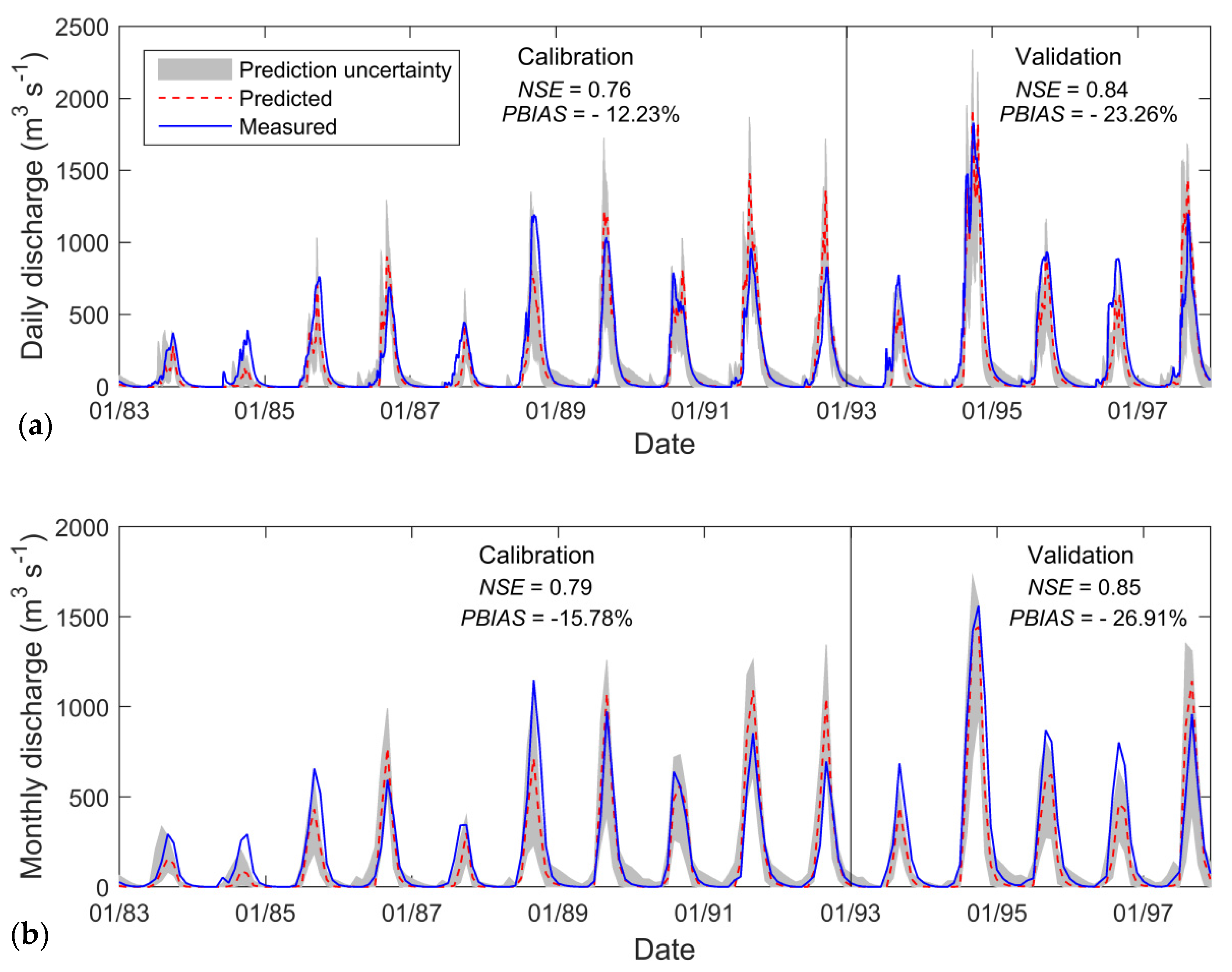
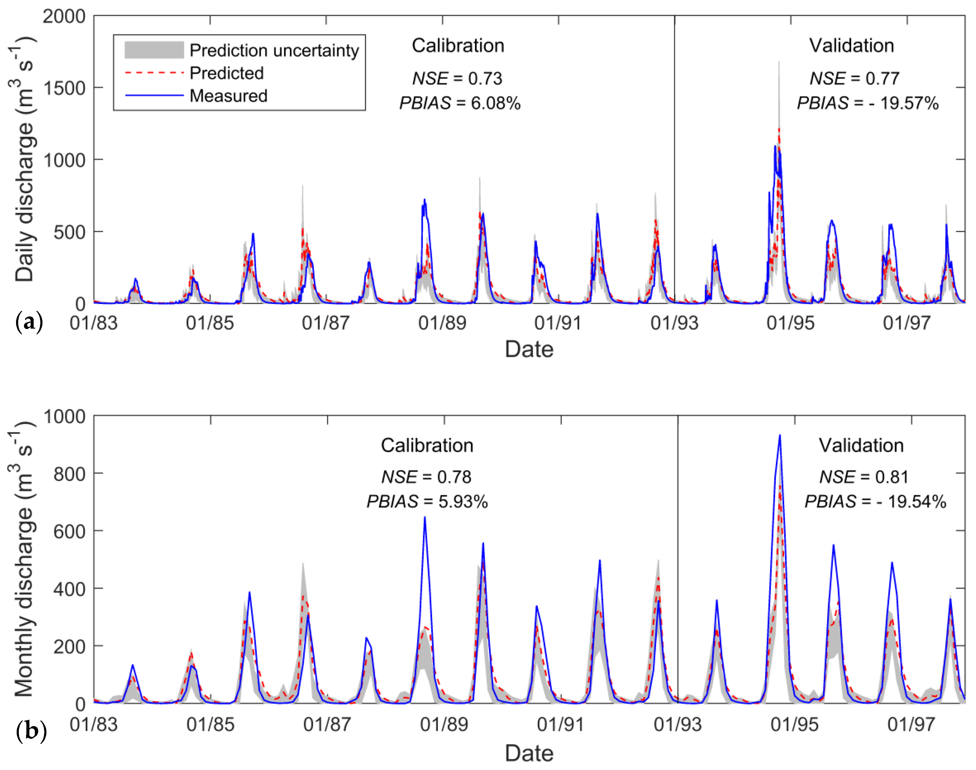
In an effort to assess the performance of the SWAT model on the Bani catchment, we calibrated and validated the model at multiple sites on daily and monthly time steps by using measured climate data. There was no statistically significant difference in model performance among time intervals. Using guidelines given in Moriasi et al. [50], the overall performance of the SWAT model in terms of NSE and R2 can be judged as very good, especially considering limited data conditions in the studied area. On a monthly basis, we obtained at the Douna outlet a NSE value equal to 0.79 for the calibration period (0.85 for the validation period). These results are greater than the ones of the studies by Schuol and Abbaspour [12], and Schuol et al. [14] at the same outlet. Schuol and Abbaspour [12] reported indeed a negative NSE (between −1 and 0) for the monthly calibration and a value ranging between 0 and 0.7 for monthly validation, while Schuol et al. [14] obtained a NSE between 0 and 0.70 for both monthly calibration and validation. However, Laurent and Ruelland [23] reported a greater performance (NSE values varying between 0.81 and 0.91 for calibration and validation period, respectively) but on a coarser time step (average annual basis). The water balance is less well simulated, especially for monthly time step with a PBIAIS greater than 25% in absolute value.
The quantified prediction uncertainty is surprisingly satisfactory (Table 6). At the end of the daily calibration, the model was able to account for 61% of observed discharge data (65% for monthly calibration) in a narrow uncertainty band. These results are close to the result of Schuol et al. [14] who estimated the observed discharge data bracketed by the 95PPU between 60% and 80% for monthly calibration (40% and 60% for monthly validation). However, one explanation that could be attributed to the small uncertainty band we obtained is that model predictive uncertainty derived by GLUE depends largely on the threshold value to separate “behavioral” from “non-behavioral” parameter sets [63,64].
This means, a high threshold value (as in this case) will generally lead to a narrower uncertainty band [65,66,67] but this will be achieved at the cost of bracketing less observed data within the 95PPU band. In addition, GLUE accounts partly for uncertainty due to the possible non-uniqueness (or equifinality) of parameter sets during calibration and could therefore underestimate total model uncertainty [68]. For instance, Sellami et al. [69] showed that the GLUE predictive uncertainty band was larger and surrounded more observation data when uncertainty in the discharge data was explicitly considered. Engeland and Gottschalk [70] demonstrated that the conceptual water balance model structural uncertainty was larger than parameter uncertainty. In spite of all the aforementioned limitations of GLUE, we succeeded in enclosing interestingly most of the observed data within a narrow uncertainty band (the sought adequate balance between the two indices) hence increasing confidence in model results. These are encouraging results showing, on one hand, the good performance of the SWAT model on a large Soudano-Sahelian catchment under limited data and varying climate conditions and, on the other hand, the capability of observed climate and hydrological input data of this catchment, even though contested, to provide reliable information about hydro-meteorological systems prevailing in the region.
It has been also noted that the model did not perform well during the year 1984 particularly (lower performance and larger uncertainty). This loss of performance can be attributed to the disruption in rainfall-runoff relationship consequence of consecutive years of drought, which has prevailed in the beginning of the 80s. The over-predicted PET on the Bani catchment could be attributed to the Hargreaves method, which could give a greater estimate of PET than it actually is. Ruelland et al. [28] applied a temperature-based method given by Oudin et al. [71] and provided a similar estimate of PET (1723 mm) than the values calculated herein by the Penman and pan evaporation methods hence corroborating our results. These results demonstrated the valuable of pan evaporation measurements for estimating PET and that the simple pan evaporation method appears to be suited for application in the study area and can be used when all the climatic data required by the Penman method are missing.
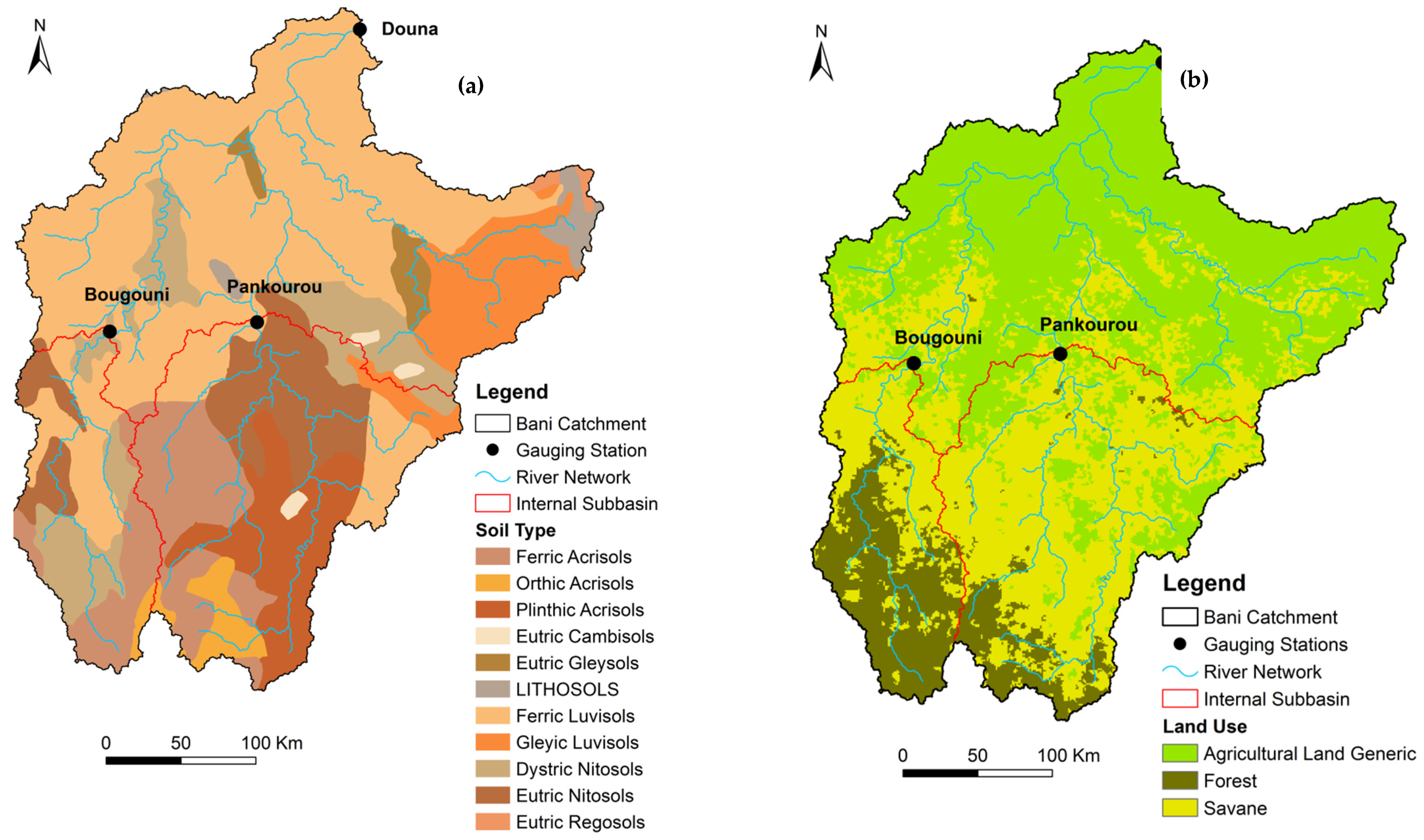
As far as biomass is concerned, the underestimation of this component in savannah could be explained by inappropriate specification of all categories in the land use map grid to be modeled by SWAT as savannah or inaccurate savannah characteristics added in the SWAT database, directly affecting biomass production such as BIO_E and LAI parameters, among others.

4.2. Impact of Spatial and Temporal Scales on the Model Uncertainty

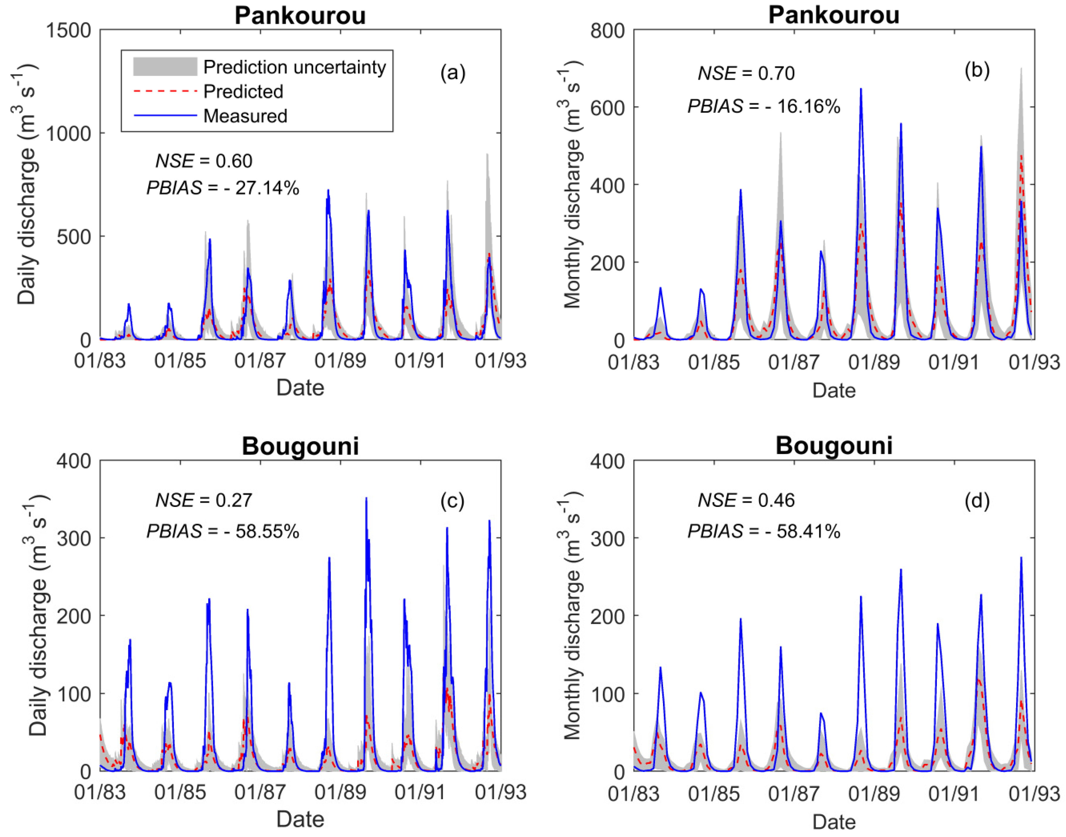
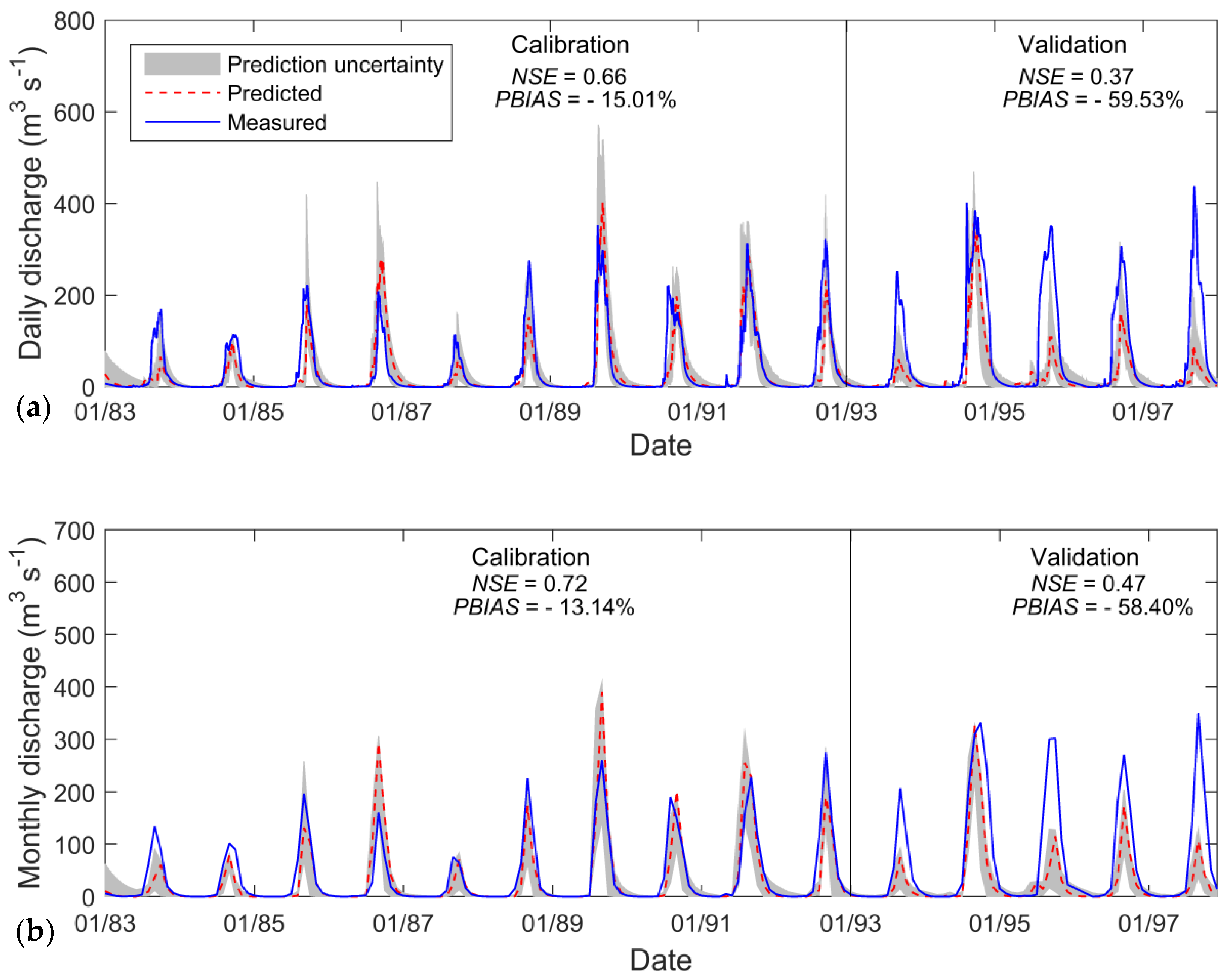
Results showed that transferring the model parameters from the catchment outlet (Douna) to the internal gauging stations performs reasonably well only in the case of similarity between donor and target catchments. The case of catchments controlled by Douna and Pankourou gives a clear example of such physical proximity where precipitation, soil and land use vary smoothly between both catchments. However, the SWAT model parameters determined at the outlet could not reproduce well the measured discharge at Bougouni mainly due to more significant spatial dissimilarities. Bougouni is indeed situated in a more humid zone and dominated by forest whereas Douna is more arid. Moreover, it has been demonstrated that the individual calibration at subcatchment scale has led to a narrower uncertainty band and more observed discharge data enclosed in it, which is the sought adequate balance between the two indices. Hence, predictive uncertainty was found to decrease with decreasing spatial scale. This finding can be attributed to the presence of less heterogeneity in hydrological variables in smaller catchments. These results showed the importance of the calibration of hydrological models at finer spatial scale to ensure that predominant processes in each subcatchment are captured, and this is particularly relevant in case of large-area global catchments. Concerning the effect of temporal scale, we demonstrated that the validation period is characterized by less predictive uncertainty as opposed to the calibration period. One explanation that can be given is the fact that 1993-1997 constitutes a more humid period than 1983-1992 and is characterized, therefore, by less variability in precipitation. In contrast, when moving from daily to monthly calibration, the uncertainty of the model, in terms of uncertainty band width, increased. This could be attributed to the cumulative effect of uncertainty in daily discharge data used to compute monthly discharge, resulting therefore in larger monthly uncertainty. Overall, due to decreasing prediction uncertainty with decreasing spatial and temporal scales, it is germane to develop on the basin a more efficient system of hydro-meteorological data collection to account for spatial and temporal variabilities in hydro-meteorological systems prevailing in the region, especially under changing climate and land use conditions.

4.3. Advance in Understanding of Hydrological Processes

The GSA confirms what has already been reported on and around the Bani catchment about the contribution of hydrological processes to streamflow generation. In order to better understand the origin of flows at Kolondieba (a tributary of the Bani River), Dao et al. [72] showed that Groundwater contribution to the hydrodynamic equilibrium at the outlet of watershed Kolondieba is small and the direct flow from the soil surface governs the runoff process. This fact can be explained by the double impact of a general impoverishment of shallow aquifers due to reduction in precipitation in West Africa in general since the great drought of the 70s as well as a concurrent increase of the recession coefficient of the Bani river as demonstrated by Bamba et al. [32] and Mahé [73] with a decrease of baseflow contribution to total flow in absolute and relative values as corollary.

4.4. Spatial Performance

The results of different calibration and validation techniques showed varying predictive abilities of the SWAT model through scales. Firstly, it can be derived from these findings that model performance in terms of NSE and R2 was higher on the watershed-wide level than on the sub-watershed level. However, this could be attributed to compensation between positive and negative errors of processes occurring at a larger scale [74,75]. This suggests that calibrating a model only at the basin outlet leads to an overconfidence in its performance than at the sub-basin scale. Secondly, individual calibration of subcatchment processes expectedly improved model accuracy in predicting flows at the internal gauging stations, due to reducing heterogeneities with downsizing space [76], and is especially beneficent while the donor and receiver catchments are substantially different. Finally, predictive uncertainty appears to decrease with reducing spatial scale, but increases with humidity as shown by the lower performance recorded at Bougouni. The inability of the model to perform during the validation period at Bougouni could be attributed to the structure of the validation period which is substantially different to that of calibration, and is solely composed by average to wet years while in contrast, the occurrence of dry, average, and wet years during the calibration period is noted.
These results have an important role to play in the calibration and validation approaches of large-area watershed models and constitutes a first step to model parameter regionalization for prediction in ungauged basins.
Generally speaking, it is well known that in recent decades the Niger River basin has suffered from a serious degradation of its natural resources, which in turn lead to severe environmental issues. To this end, different agreements and collaborations on water and climate data sharing have been established between the 9 countries sharing the basin through different national and international programs. Thus, the need to reinforce the existing framework of integrated, coordinated, and sustainable water management strategies in the Bani basin and therefore the Niger River Basin become more urgent than ever.
Therefore, this study is a step in that long-term direction, where an integrated water management tool has been developed and validated spatially on the Bani catchment, which allows investigation of future effects of land use and climate change scenarios on water resources.

5. Conclusions

In this study, the performance of the widely-used SWAT model was evaluated on the Bani catchment using both split-sample and split-location calibration and validation techniques on daily and monthly intervals. The model was calibrated at the Douna outlet and at two internal stations. Freely available global data and daily observed climate and discharge data were used as inputs for model simulation and calibration. Calibration, validation, uncertainty, and sensitivity analyses were performed with GLUE within SWAT-CUP. Both graphical and statistical techniques were used for hydrologic calibration results evaluation. Evapotranspiration and biomass production outputs were verified and compared to regional values to make sure these components were reasonably predicted. Sensitivity analysis contributed to a better understanding of the hydrological processes occurring at the study area.
Final results showed a good SWAT model performance to predict daily as well as monthly discharge at Douna with acceptable predictive uncertainty despite the poor data density and the high gradient of climate and land use characterizing the study catchment. However, the daily calibration resulted in less predictive uncertainty than the monthly calibration. The performance of the model is somehow lower at an internal sub-catchments level when the global parameter sets are applied, especially at the one with higher humidity and dominated by forest. However, subcatchment calibration induced an increase of model performance at intermediate gauging stations as well as a decrease of total uncertainty. With regard to predicted PET, this component is overestimated by the model when the Hargreaves method is applied in that specific region while biomass production remained low in the savannah land use category. The GSA revealed the predominance of surface and subsurface processes in the streamflow generation of the Bani River.
Overall, this study has shown the validity of the SWAT model for representing globally hydrological processes of a large-scale Soudano-Sahelian catchment in West Africa. Given the high spatial variability of climate, soil, and land use characterizing the catchment, additional calibration is however needed at subcatchment level to ensure that predominant processes are captured in each subcatchment. Accordingly, the importance of spatially distributed hydrological measurements is demonstrated and constitutes the backbone of any type of progress in hydrological process understanding and modeling. The calibrated SWAT model for the Bani can be used to assess the current and future impacts of climate and land use change on water resources of the catchment, increasingly necessary information awaited by water resources managers. Knowing this information, a strategy of adaptation in response to the current and future impacts can be clearly proposed and the vulnerability of the population can therefore be reduced. More widely, this impact study can increase the transferability of the model parameters from the Bani subcatchment to another ungauged basin with some similarities, and then predicting discharge without the need of any measurement. These findings are very useful, especially in West Africa, where many river basins are ungauged or poorly gauged.

Acknowledgments

Authors are extremely grateful to AGRHYMET for providing the climatic database. We would like also to thank Kone Soungalo for climate data on the Ivorian part of the Bani basin and Francois Laurent for soil and land use databases.

Funding

This study was funded by the German Ministry of Education and Research (BMBF) through the West African Science Service Centre on Climate Change and Adapted Land Use (WASCAL; www.wascal.org) that supports the Graduate Research Program Climate Change and Water Resources at the University of Abomey-Calavi. Additional funds were provided by AGRHYMET through the French Global Environment Facility (FFEM/CC) project.

Author Contributions

All authors designed the objectives and methods of the study. J. C. Begou, P. Bazie, and A. Afouda collected the climatological and hydrological datasets required for the model. J. C. Begou, S. Jomaa, S. Benabdallah, and M. Rode conducted the model setup and performed the simulations. All authors analyzed the obtained data. J. C. Begou prepared the manuscript with contributions from all co-authors. All authors read and approved the final manuscript.

Conflicts of Interest

The authors declare no conflict of interest.

References

  1. Pomeroy, J.W.; Spence, C.; Whitfield, P.H. Putting prediction in ungauged basins into practice. In Putting Prediction in Ungauged Basins into Practice; Canadian Water Resources Association: Ottawa, ON, Canada, 2013; pp. 1–12. [Google Scholar]
  2. Sivapalan, M.; Takeuchi, K.; Franks, S.W.; Gupta, V.K.; Karambiri, H.; Lakshmi, V.; Liang, X.; McDonnell, J.J.; Mendiondo, E.M.; O’Connell, P.E.; et al. Iahs decade on predictions in ungauged basins (PUB), 2003–2012: Shaping an exciting future for the hydrological sciences. Hydrol. Sci. J. 2003, 48, 857–880. [Google Scholar] [CrossRef]
  3. Bormann, H.; Diekkrüger, B. Possibilities and limitations of regional hydrological models applied within an environmental change study in Benin (West Africa). Phys. Chem. Earth Parts A/B/C 2003, 28, 1323–1332. [Google Scholar] [CrossRef]
  4. Kapangaziwiri, E.; Hughes, D.A.; Wagener, T. Incorporating uncertainty in hydrological predictions for gauged and ungauged basins in Southern Africa. Hydrol. Sci. J. 2012, 57, 1000–1019. [Google Scholar] [CrossRef]
  5. Mazvimavi, D.; Meijerink, A.M.J.; Savenije, H.H.G.; Stein, A. Prediction of flow characteristics using multiple regression and neural networks: A case study in Zimbabwe. Phys. Chem. Earth Parts A/B/C 2005, 30, 639–647. [Google Scholar] [CrossRef]
  6. Minihane, M. Estimating mean monthly streamflow in the Lugenda River, Northern Mozambique. In Putting Prediction in Ungauged Basins into Practice; Canadian Water Resources Association: Ottawa, ON, Canada, 2013; pp. 185–196. [Google Scholar]
  7. Ndomba, P.; Mtalo, F.; Killingtveit, A. SWAT model application in a data scarce tropical complex catchment in Tanzania. Phys. Chem. Earth Parts A/B/C 2008, 33, 626–632. [Google Scholar] [CrossRef]
  8. Nkamdjou, L.S.; Bedimo, J.B. Critique des Donnees Hydrometriques du Bassin du Niger: Rapport Preliminaire; Niger Basin Authority: Niamey, Niger, 2008; p. 28.
  9. IPCC. Climate Change 2014: Impacts, Adaptation, and Vulnerability. Part B: Regional Aspects; Barros, V.R., Field, C.B., Dokken, D.J., Mastrandrea, M.D., Mach, K.J., Bilir, T.E., Chatterjee, M., Ebi, K.L., Estrada, Y.O., Genova, R.C., et al., Eds.; Cambridge University Press: Cambridge, UK; New York, NY, USA, 2014; p. 688. [Google Scholar]
  10. Wagener, T.; Wheater, H.S.; Gupta, H.V. Rainfall-Runoff Modelling in Gauged and Ungauged Catchments; Imperial College Press: London, UK, 2004; p. 332. [Google Scholar]
  11. Amadou, A.; Djibo Abdouramane, G.; Ousmane, S.; Sanda Ibrah, S.; Sittichok, K. Changes to flow regime on the Niger River at Koulikoro under a changing climate. Hydrol. Sci. J. 2015, 60, 1709–1723. [Google Scholar]
  12. Schuol, J.; Abbaspour, K.C. Calibration and uncertainty issues of a hydrological model (SWAT) applied to West Africa. Adv. Geosci. 2006, 9, 137–143. [Google Scholar] [CrossRef]
  13. Schuol, J.; Abbaspour, K.C. Using monthly weather statistics to generate daily data in a SWAT model application to West Africa. Ecol. Model. 2007, 201, 301–311. [Google Scholar] [CrossRef]
  14. Schuol, J.; Abbaspour, K.C.; Srinivasan, R.; Yang, H. Estimation of freshwater availability in the West African sub-continent using the SWAT hydrologic model. J. Hydrol. 2008, 352, 30–49. [Google Scholar] [CrossRef]
  15. Schuol, J.; Abbaspour, K.C.; Yang, H.; Srinivasan, R.; Zehnder, A.J.B. Modeling blue and green water availability in Africa. Water Resour. Res. 2008, 44, 1–18. [Google Scholar] [CrossRef]
  16. Sittichok, K.; Gado Djibo, A.; Seidou, O.; Moussa Saley, H.; Karambiri, H.; Paturel, J. Statistical seasonal rainfall and streamflow forecasting for the Sirba watershed, West Africa, using sea surface temperatures. Hydrol. Sci. J. 2014, 61, 1700–1712. [Google Scholar] [CrossRef]
  17. Awotwi, A.; Yeboah, F.; Kumi, M. Assessing the impact of land cover changes on water balance components of White Volta Basin in West Africa. Water Environ. J. 2015, 29, 259–267. [Google Scholar] [CrossRef]
  18. Guzinski, R.; Kass, S.; Huber, S.; Bauer-Gottwein, P.; Jensen, I.; Naeimi, V.; Doubkova, M.; Walli, A.; Tottrup, C. Enabling the use of earth observation data for integrated water resource management in Africa with the water observation and information system. Remote Sens. 2014, 6, 7819–7839. [Google Scholar] [CrossRef] [Green Version]
  19. Sood, A.; Muthuwatta, L.; McCartney, M. A SWAT evaluation of the effect of climate change on the hydrology of the Volta River Basin. Water Int. 2013, 38, 297–311. [Google Scholar] [CrossRef]
  20. Bossa, A.Y.; Diekkrüger, B.; Giertz, S.; Steup, G.; Sintondji, L.O.; Agbossou, E.K.; Hiepe, C. Modeling the effects of crop patterns and management scenarios on N and P loads to surface water and groundwater in a semi-humid catchment (West Africa). Agric. Water Manag. 2012, 115, 20–37. [Google Scholar] [CrossRef]
  21. Bossa, A.Y.; Diekkrüger, B.; Igué, A.M.; Gaiser, T. Analyzing the effects of different soil databases on modeling of hydrological processes and sediment yield in Benin (West Africa). Geoderma 2012, 173–174, 61–74. [Google Scholar]
  22. Sintondji, L.O.; Barnabé, Z.; Ahouansou, D.M.; Vissin, W.E.; Agbossou, K.E. Modelling the water balance of ouémé catchment at the savè outlet in Benin: Contribution to the sustainable water resource management. Int. J. AgriSci. 2014, 4, 74–88. [Google Scholar]
  23. Laurent, F.; Ruelland, D. Modélisation à base physique de la variabilité hydroclimatique à l’échelle d’un grand bassin versant tropical. In Global Change: Facing Risks and Threats to Water Resources, Proceedings of the sixth world FRIEND conference, Fez, Morroco, 25–29 October 2010; International Association of Hydrological Sciences (IAHS): Wallingford, UK, 2010; pp. 474–484. [Google Scholar]
  24. Ruelland, D.; Ardoin-Bardin, S.; Billen, G.; Servat, E. Sensitivity of a lumped and semi-distributed hydrological model to several methods of rainfall interpolation on a large basin in West Africa. J. Hydrol. 2008, 361, 96–117. [Google Scholar]
  25. Masih, I.; Maskey, S.; Uhlenbrook, S.; Smakhtin, V. Assessing the impact of areal precipitation input on streamflow simulations using the SWAT model. J. Am. Water Resour. Assoc. 2011, 47, 179–195. [Google Scholar] [CrossRef]
  26. Paturel, J.E.; Ouedraogo, M.; Mahé, G.; Servat, E.; Dezetter, A.; Ardoin, S. The influence of distributed input data on the hydrological modelling of monthly river flow regimes in West Africa. Hydrol. Sci. J. 2003, 48, 881–890. [Google Scholar]
  27. Food and Agriculture Organization of the United Nations (FAO). Digital Soil Map of the World and Derived Soil Properties; Version 3.6; Land and Water Development Division, FAO: Rome, Italy, 2003. [Google Scholar]
  28. Ruelland, D.; Ardoin-Bardin, S.; Collet, L.; Roucou, P. Simulating future trends in hydrological regime of a large sudano-sahelian catchment under climate change. J. Hydrol. 2012, 424–425, 207–216. [Google Scholar]
  29. Loveland, T.R.; Reed, B.C.; Brown, J.F.; Ohlen, D.O.; Zhu, Z.; Yang, L.; Merchant, J.W. Development of a global land cover characteristics database and IGBP DISCover from 1 km AVHRR data. Int. J. Remote Sens. 2000, 21, 1303–1330. [Google Scholar]
  30. L’Hote, Y.; Mahé, G.; Some, B.; Triboulet, J.P. Analysis of a sahelian annual rainfall index from 1896 to 2000; the drought continues. Hydrol. Sci. J. 2002, 47, 563–572. [Google Scholar] [CrossRef]
  31. Mahé, G.; Olivry, J.-C.; Dessouassi, R.; Orange, D.; Bamba, F.; Servat, E. Relations eaux de surface-eaux souterraines d’une rivière tropicale au Mali. Comptes Rendus de l’Académie des Sciences Series IIA Earth Planet. Sci. 2000, 330, 689–692. [Google Scholar] [CrossRef]
  32. Bamba, F.; Mahe, G.; Bricquet, J.P.; et Olivry, J.C. Changements climatiques et variabilite des ressources en eau des bassins du haut niger et de la cuvette lacustre. XIIèmes journees hydrologiques de l’orstom 1996, 10–11, 1–27. [Google Scholar]
  33. Ruelland, D.; Guinot, V.; Levavasseur, F.; Cappelaere, B. Modelling the longterm impact of climate change on rainfall-runoff processes over a large sudano-sahelian catchment. In New Approaches to Hydrological Prediction in Data Sparse Regions, Proceedings of the Symposium HS.2 at the Joint Convention of The International Association of Hydrological Sciences (IAHS) and The International Association of Hydrogeologists (IAH), Hyderabad, India, 6–12 September 2009; IAHS: Wallingford, UK, 2009; pp. 59–68. [Google Scholar]
  34. Arnold, J.G.; Srinivasan, R.; Muttiah, R.S.; Williams, J.R. Large area hydrologic modeling and assessment part i: Model development. J. Am. Water Resour. Assoc. 1998, 34, 73–89. [Google Scholar] [CrossRef]
  35. Winchell, M.; Srinivasan, R.; di Luzio, M.; Arnold, J.G. Arcswat Interface for SWAT. 2012 User’s Guide; Soil and Water Research Laboratory, USDA Agricultural Research Service: Temple, TX, USA, 2013; p. 459.
  36. Arnold, J.G.; Kiniry, J.R.; Srinivasan, R.; Williams, J.R.; Haney, E.B.; Neitsch, S.L. Soil and Water Assessment Tool Input/Output Documentation: Version 2012; Texas Water Resources Institute Technical Report: College Station, TX, USA, 2012; Volume TR-439. [Google Scholar]
  37. Neitsch, S.L.; Arnold, J.G.; Kiniry, J.R.; Williams, J.R. Soil and Water Assessment Tool Theoretical Documentation: Version 2009; Technical Report No. 406; Texas Water Resources Institute Texas: College Station, TX, USA, 2011. [Google Scholar]
  38. Bouraoui, F.; Benabdallah, S.; Jrad, A.; Bidoglio, G. Application of the SWAT model on the Medjerda River Basin (Tunisia). Phys. Chem. Earth Parts A/B/C 2005, 30, 497–507. [Google Scholar] [CrossRef]
  39. Ouessar, M.; Bruggeman, A.; Abdelli, F.; Mohtar, R.H.; Gabriels, D.; Cornelis, W.M. Modelling water-harvesting systems in the arid south of Tunisia using SWAT. Hydrol. Earth Syst. Sci. 2009, 13, 2003–2021. [Google Scholar] [CrossRef]
  40. World Meteorological Organization (WMO). WMO-No.100. Guide to Climatological Practices, 3rd ed.; WMO: Geneva, Switzerland, 2011. [Google Scholar]
  41. Boisramé, G. WGN Excel Macro. Available online: http://swat.Tamu.Edu/software/links/ (accessed on 25 April 2016).
  42. USGS Hydrosheds. Available online: http://hydrosheds.cr.usgs.gov/dataavail.php (accessed on 26 April 2016).
  43. Waterbase. Available online: http://www.waterbase.org/resources.html (accessed on 26 April 2016).
  44. FAO. Available online: http://www.fao.org/geonetwork/srv/en/main.home (accessed on 26 April 2016).
  45. Nash, J.E.; Sutcliffe, J.V. River flow forecasting through conceptual models part I—A discussion of principles. J. Hydrol. 1970, 10, 282–290. [Google Scholar] [CrossRef]
  46. Moussa, R.; Chahinian, N.; Bocquillon, C. Distributed hydrological modelling of a mediterranean mountainous catchment—Model construction and multi-site validation. J. Hydrol. 2007, 337, 35–51. [Google Scholar] [CrossRef]
  47. Robson, B.J.; Dourdet, V. Prediction of sediment, particulate nutrient and dissolved nutrient concentrations in a dry tropical river to provide input to a mechanistic coastal water quality model. Environ. Model. Softw. 2015, 63, 97–108. [Google Scholar] [CrossRef]
  48. Abbaspour, K.C. SWAT-Cup 2012: SWAT Calibration and Uncertainty Programs—A User Manual; Eawag, Swiss Federal Institute of Aquatic Science and Technology: Duebendorf, Switzerland, 2014; p. 106. [Google Scholar]
  49. Beven, K.; Binley, A. The future of distributed models: Model calibration and uncertainty prediction. Hydrol. Process. 1992, 6, 279–298. [Google Scholar] [CrossRef]
  50. Moriasi, D.N.; Arnold, J.G.; van Liew, M.W.; Bingner, R.L.; Harmel, R.D.; Veith, T.L. Model evaluation guidelines for systematic quantification of accuracy in watershed simulations. Trans. ASABE 2007, 50, 885–900. [Google Scholar] [CrossRef]
  51. Arnold, J.G.; Allen, P.M.; Muttiah, R.; Bernhardt, G. Automated base flow separation and recession analysis techniques. Ground Water 1995, 33, 1010–1018. [Google Scholar] [CrossRef]
  52. Arnold, J.G.; Allen, P.M. Automated methods for estimating baseflow and ground water recharge from streamflow records. J. Am. Water Resour. Assoc. 1999, 35, 411–424. [Google Scholar] [CrossRef]
  53. Betrie, G.D.; Mohamed, Y.A.; van Griensven, A.; Srinivasan, R. Sediment management modelling in the Blue Nile Basin using SWAT model. Hydrol. Earth Syst. Sci. 2011, 15, 807–818. [Google Scholar] [CrossRef]
  54. Van Griensven, A.; Meixner, T.; Grunwald, S.; Bishop, T.; Diluzio, M.; Srinivasan, R. A global sensitivity analysis tool for the parameters of multi-variable catchment models. J. Hydrol. 2006, 324, 10–23. [Google Scholar] [CrossRef]
  55. Zhang, X.; Srinivasan, R.; Liew, M.V. Multi-site calibration of the SWAT model for hydrologic modeling. Trans. ASABE 2008, 51, 2039–2049. [Google Scholar] [CrossRef]
  56. Arnold, J.G.; Moriasi, D.N.; Gassman, P.W.; Abbaspour, K.C.; White, M.J.; Srinivasan, R.; Santhi, C.; Harmel, R.D.; Griensven, A.V.; Liew, M.W.V.; et al. SWAT: Model use, calibration, and validation. Trans. ASABE 2012, 55, 1491–1508. [Google Scholar] [CrossRef]
  57. Abbaspour, K.C.; Johnson, C.A.; van Genuchten, M.T. Estimating uncertain flow and transport parameters using a sequential uncertainty fitting procedure. Vadose Zone J. 2004, 3, 1340–1352. [Google Scholar] [CrossRef]
  58. Hargreaves, G.L.; Hargreaves, G.H.; Riley, J.P. Agricultural benefits for Senegal River Basin. J. Irrig. Drain. Eng. 1985, 111, 113–124. [Google Scholar] [CrossRef]
  59. Allen, R.G.; Pereira, L.S.; Raes, D.; Smith, M. Crop Evapotranspiration-Guidelines for Computing Crop Water Requirements-FAO Irrigation and Drainage Paper 56; Food and Agriculture Organization of the United Nations (FAO): Rome, Italy, 1998. [Google Scholar]
  60. Doorenbos, J.; Pruitt, W.O. Guidelines for Predicting Crop Water Requirements, Irrigation and Drainage Paper 24; Land and Water Development Division, FAO: Rome, Italy, 1975; p. 179. [Google Scholar]
  61. Brouwer, C.; Heibloem, M. Irrigation Water Management: Training Manual No. 3; Food and Agriculture Organization of the United Nations (FAO): Rome, Italy, 1986. [Google Scholar]
  62. Coulibaly, A. Profil Fourrager (Mali); Food and Agriculture Organization of the United Nations (FAO): Rome, Italy, 2003. [Google Scholar]
  63. Mantovan, P.; Todini, E. Hydrological forecasting uncertainty assessment: Incoherence of the GLUE methodology. J. Hydrol. 2006, 330, 368–381. [Google Scholar] [CrossRef]
  64. Montanari, A. Large sample behaviors of the generalized likelihood uncertainty estimation (GLUE) in assessing the uncertainty of rainfall-runoff simulations. Water Resour. Res. 2005, 41, 1–13. [Google Scholar] [CrossRef]
  65. Blasone, R.-S.; Madsen, H.; Rosbjerg, D. Uncertainty assessment of integrated distributed hydrological models using GLUE with Markov chain Monte Carlo sampling. J. Hydrol. 2008, 353, 18–32. [Google Scholar] [CrossRef] [Green Version]
  66. Viola, F.; Noto, L.V.; Cannarozzo, M.; La Loggia, G. Daily streamflow prediction with uncertainty in ephemeral catchments using the GLUE methodology. Phys. Chem. Earth Parts A/B/C 2009, 34, 701–706. [Google Scholar] [CrossRef]
  67. Xiong, L.; O’Connor, K.M. An empirical method to improve the prediction limits of the GLUE methodology in rainfall—Runoff modeling. J. Hydrol. 2008, 349, 115–124. [Google Scholar] [CrossRef]
  68. Yen, H.; Wang, X.; Fontane, D.G.; Harmel, R.D.; Arabi, M. A framework for propagation of uncertainty contributed by parameterization, input data, model structure, and calibration/validation data in watershed modelling. Environ. Model. Softw. 2014, 54, 211–221. [Google Scholar] [CrossRef]
  69. Sellami, H.; Vanclooster, M.; Benabdallah, S.; La Jeunesse, I. Assessment of the SWAT model prediction uncertainty using the GLUE approach a case study of the Chiba catchment (Tunisia). In Modeling, Simulation and Applied Optimization (ICMSAO), Proceedings of the 5th International Conference, Hammamet, Tunisia, 28–30 April 2013; Institute of Electrical and Electronics Engineers (IEEE): New York, NY, USA, 2013; pp. 1–6. [Google Scholar]
  70. Engeland, K.; Gottschalk, L. Bayesian estimation of parameters in a regional hydrological model. Hydrol. Earth Syst. Sci. 2002, 6, 883–898. [Google Scholar] [CrossRef]
  71. Oudin, L.; Hervieu, F.; Michel, C.; Perrin, C.; Andréassian, V.; Anctil, F.; Loumagne, C. Which potential evapotranspiration input for a lumped rainfall-runoff model? Part 2 towards a simple and efficient potential evapotranspiration model for rainfall-runoff modelling. J. Hydrol. 2005, 303, 290–306. [Google Scholar] [CrossRef]
  72. Dao, A.; Kamagate, B.; Mariko, A.; Seguis, L.; Maiga, H.B.; Goula Bi, T.A.; Savane, I. Deconvolution of the flood hydrograph at the outlet of watershed kolondieba in the south of Mali. Int. J. Eng. Res. Appl. 2012, 2, 1174–1181. [Google Scholar]
  73. Mahé, G. Surface/groundwater interactions in the Bani and Nakambe rivers, tributaries of the Niger and Volta Basins, West Africa. Hydrol. Sci. J. 2009, 54, 704–712. [Google Scholar] [CrossRef]
  74. Cao, W.; Bowden, W.B.; Davie, T.; Fenemor, A. Multi-variable and multi-site calibration and validation of SWAT in a large mountainous catchment with high spatial variability. Hydrol. Process. 2006, 20, 1057–1073. [Google Scholar] [CrossRef]
  75. Wellen, C.; Kamran-Disfani, A.-R.; Arhonditsis, G.B. Evaluation of the current state of distributed watershed nutrient water quality modeling. Environ. Sci. Technol. 2015, 49, 3278–3290. [Google Scholar] [CrossRef] [PubMed]
  76. Daggupati, P.; Yen, H.; White, M.J.; Srinivasan, R.; Arnold, J.G.; Keitzer, C.S.; Sowa, S.P. Impact of model development, calibration and validation decisions on hydrological simulations in West Lake Erie Basin. Hydrol. Process. 2015, 29, 5307–5320. [Google Scholar] [CrossRef]
Figure 1. Localization of the Bani catchment at the Douna outlet. The altitude and the monitoring network of the catchment are also given.
Water 08 00178 g001
Figure 2. (a) Soil attributes and (b) land use categories of the Bani catchment.
Water 08 00178 g002
Figure 3. Simulated and observed hydrographs at Douna station at (a) daily and (b) monthly timesteps along with calculated statistics on calibration and validation periods.
Water 08 00178 g003
Figure 4. Spatial validation of the SWAT model on the Bani catchment. The model was turned at Pankourou ((a) daily and (b) monthly time steps) and at Bougouni ((c) daily and (d) monthly timesteps) by using the same behavioral parameter sets determined at the Douna outlet on the period 1983–1992.
Water 08 00178 g004
Figure 5. Simulated and observed hydrographs at Pankourou station at (a) daily and (b) monthly time steps along with calculated statistics on calibration and validation periods.
Water 08 00178 g005
Figure 6. Predicted and measured discharges at Bougouni station at (a) daily and (b) monthly intervals during the calibration and validation periods with their corresponding statistics.
Water 08 00178 g006
Table 1. Input data of the SWAT model for the Bani catchment.
Data TypeDescriptionResolution/PeriodSource
Simulation Data
TopographyConditioned DEM90 mUSGS hydrosheds [42]
Land use/land coverGLCC version 21 kmWaterbase [43]
SoilFAO Soil MapScale 1:5000000FAO [44]
RiverRiver network map500 mUSGS Hydrosheds [42]
Weather dataRainfall, maximum and minimum temperatureDaily (1981-2000)AGRHYMET
Calibration/Verification Data
DischargeDischarge Daily (1983–1997)AGRHYMET/National hydrological service of Mali
PETPotential evapotranspiration10-day (1983–1998)National Meteorological Agency of Mali
EpanPan evaporationMonthly (1983–1997)AGRHYMET
Table 2. Input methods for SWAT model simulation on the Bani catchment.
CodeDescriptionMethod
General Watershed Parameters
IPETPotential Evapotranspiration methodHargreaves
IEVENTRainfall/runoff/routing optionDaily Rainfall/CN runoff/Daily routing
ICNDaily Curve Number calculation methodSoil moisture (Plant ET at Bougouni)
IRTE Channel water routing methodVariable storage
SWAT Simulation
Period of simulation-1981–2000
NYSKIP Warm-up periodTwo years (1981 and 1982)
Table 3. Model performance statistics for the Bani catchment at Douna, Pankourou, and Bougouni discharge gauging stations.
Time Step Calibration (1983–1992)Validation (1993–1997)
CriterionDounaPankourouBougouniDounaPankourouBougouni
DailyNSE0.760.730.660.850.770.37
R20.790.740.680.870.830.57
PBIAS (%)−12.236.08−15.01−23.26−19.57−59.53
MonthlyNSE0.790.780.720.850.810.47
R20.820.780.760.880.910.68
PBIAS (%)−15.785.93−13.14−26.91−19.54−58.40
Table 4. Average annual basin values of precipitation (P), evapotranspiration (ET), potential evapotranspiration (PET), and biomass as SWAT outputs on the Bani catchment.
PeriodP (mm)ET (mm)PET (mm) aBiomass (ton ha−1)
Agricultural Land GenericSavannahForest
Calibration (1983–1992)96089519261.180.273.09
Validation (1993–1997)105097519251.720.535.51
a Average annual PET estimated by the Hargreaves method (herein used by SWAT).
Table 5. Summary of the SWAT model parameters calibrated on the Bani catchment at Douna on a daily time interval.
ParameterDescriptionInput Calibration RangeCalibrated Parameters: Best Parameter Value [Range]Global Sensitivity Analysis
t-Statp-Value
CN2SCS runoff curve number II (-)±20%−0.155 [−0.199; 0.102]−54.030830.00000
OV_NManning’s “n” value for overland flow (-)0.01–3023.153 [3.061; 29.915]11.416030.00000
SLSUBBSNAverage slope length (m)10–150149.808 [12.677; 149.924]8.873520.00000
ESCOSoil evaporation compensation factor (-)0.01–10.958 [0.768; 0.991]−6.088800.00000
SOL_AWCAvailable water capacity of the soil layer (mm H2O/mm sol)±20%0.140 [−0.199; 0.197]2.898640.00376
GW_DELAYGroundwater delay (days)0.0–504.938 [0.487; 49.823]1.813410.06980
GWQMNThreshold depth of water in the shallow aquifer required for return flow to occur (mm H2O)0.0–40003082.500 [0.043; 3995.710]−1.518530.12891
REVAPMNThreshold depth of water in the shallow aquifer for “revap” to occur (mm H2O)0–500173.709 [0.636; 499.845]−0.649390.51610
RCHRG_DPDeep aquifer percolation fraction (-)0–10.346 [0.001; 0.999]0.464080.64260
GW_REVAPGroundwater “revap” coefficient (-)0.02–0.20.190 [0.021; 0.199]−0.126130.89963
SURLAGSurface runoff lag coefficient (-)0.05–2420.219 [0.076; 23.878]−0.074330.94075
ALPHA_BF*Baseflow alpha factor (d−1) 0.0340.034NDND
* Determined on observed discharges by applying the baseflow filter program. ND: Not Determined.
Table 6. Predictive uncertainty indices of the SWAT model for the Bani catchment at Douna, Pankourou, and Bougouni discharge gauging stations.
Time Step Calibration (1983–1992)Validation (1993–1997)
CriterionDounaPankourouBougouniDounaPankourouBougouni
DailyP-factor0.610.680.600.620.630.51
R-factor0.590.410.570.510.290.35
MonthlyP-factor0.650.710.580.700.670.55
R-factor0.650.450.540.550.310.32

