
Experimental and Numerical Study of Bottom Rack Occlusion by Flow with Gravel-Sized Sediment. Application to Ephemeral Streams in Semi-Arid Regions


Abstract
:1. Introduction
- ▪
- Bar clearance higher than the d90 grain size transported during flood events. Recommended spacing between bars is 0.100–0.120 m in general cases (0.020–0.030 m in cases of water power plants).
- ▪
- Longitudinal rack slope 20%–60% to reduce the probability of sediment deposition over it.
- ▪
- Increment of the opening area of the rack by consideration of the surface partially clogging with a factor of around 1.5–2.0.
- ▪
- Construction of an upstream stilling basin that regulates the size of the incoming sediments.
2. Experimental Setting
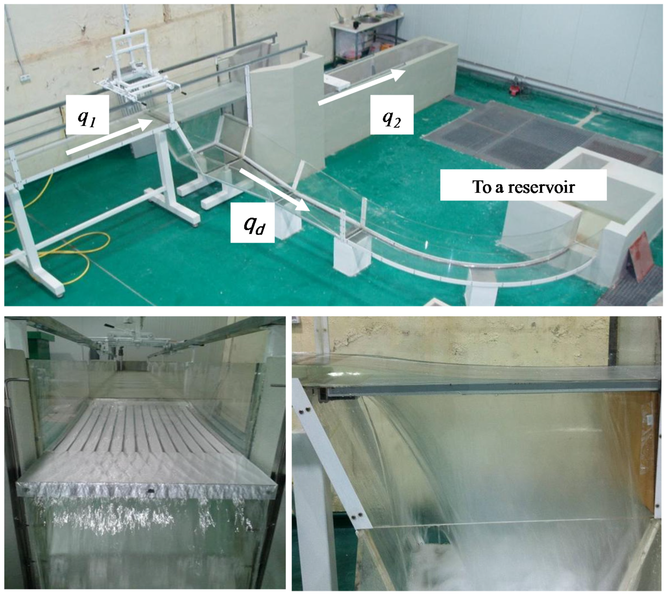
2.1. Physical Device
2.2. Clear Water Experimental Tests
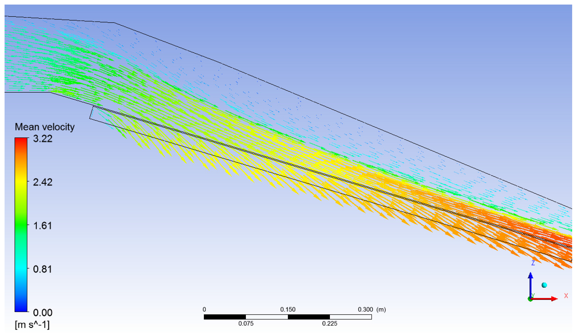
2.3. Numerical Simulations with Clear Water
2.4. Sediment Experimental Tests
3. Results and Discussion
3.1. Clear Water Tests
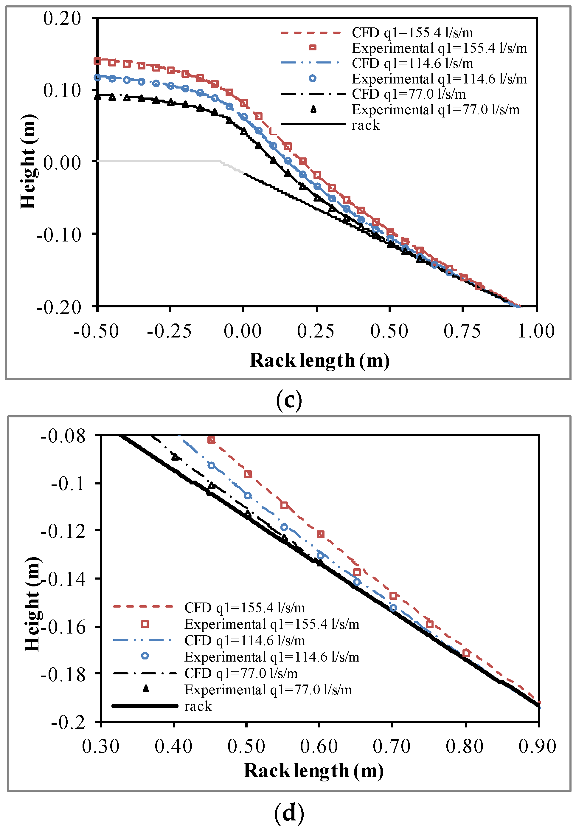
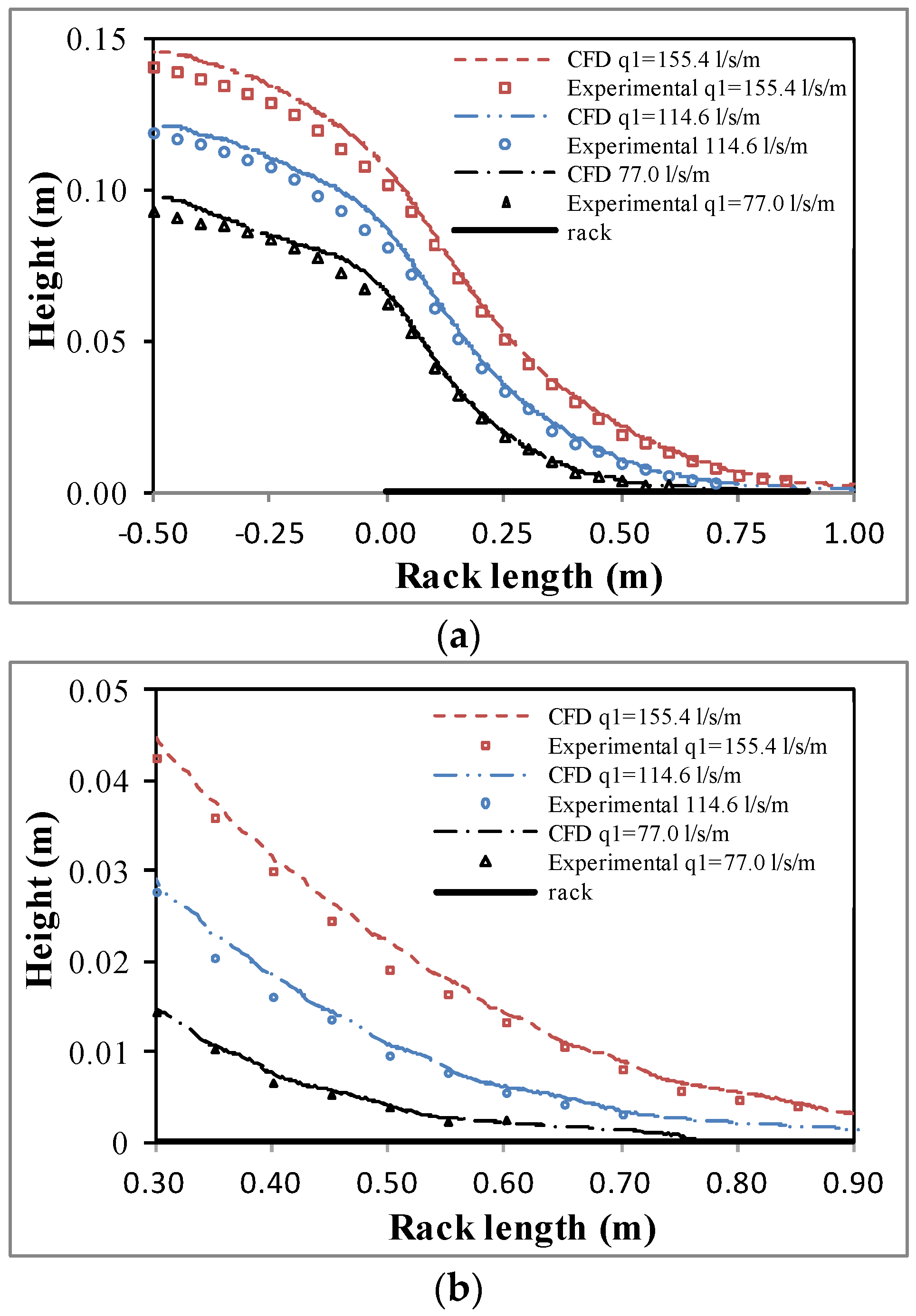
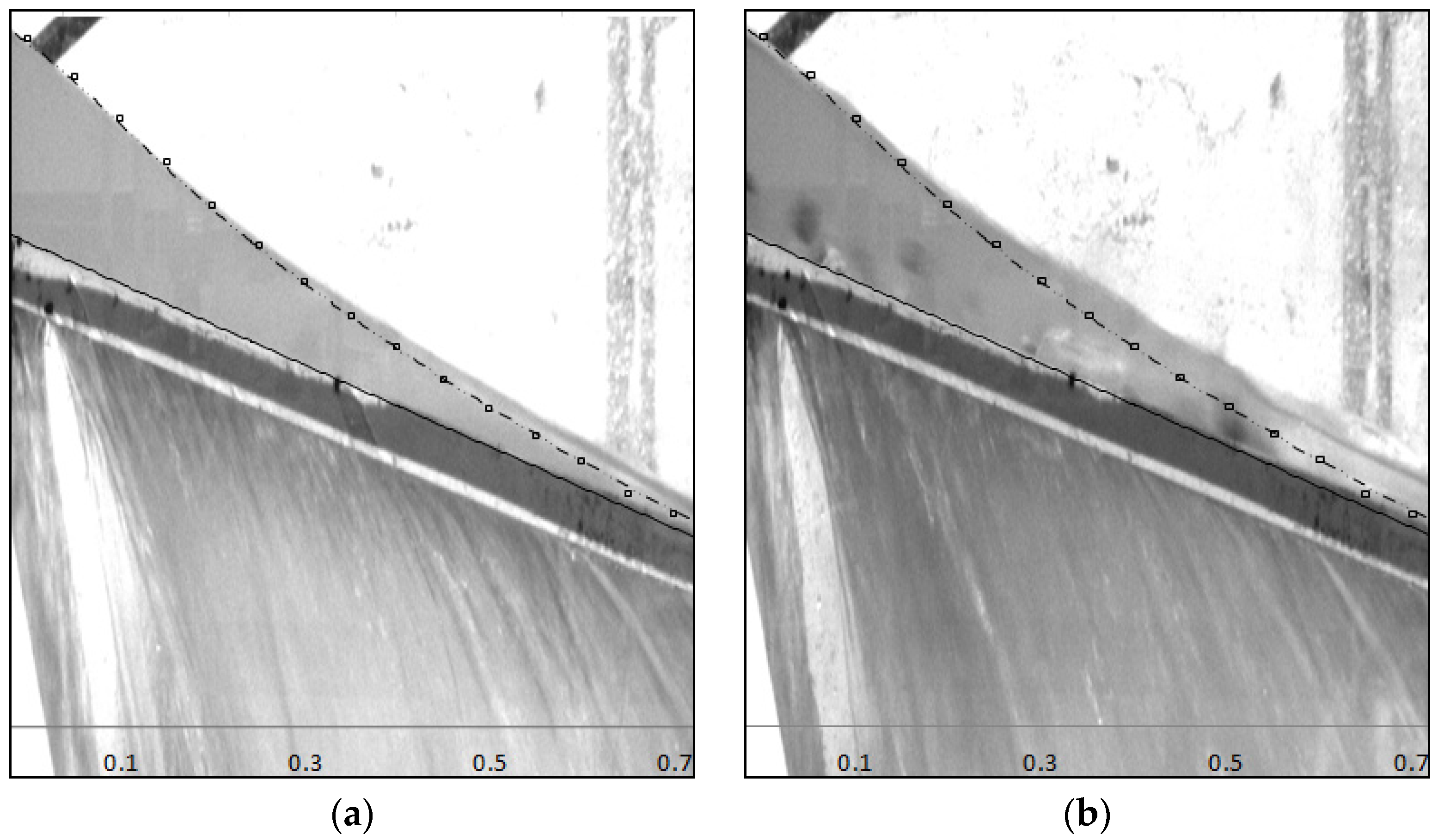
3.1.1. Longitudinal Flow Profile
3.1.2. Discharge Coefficient
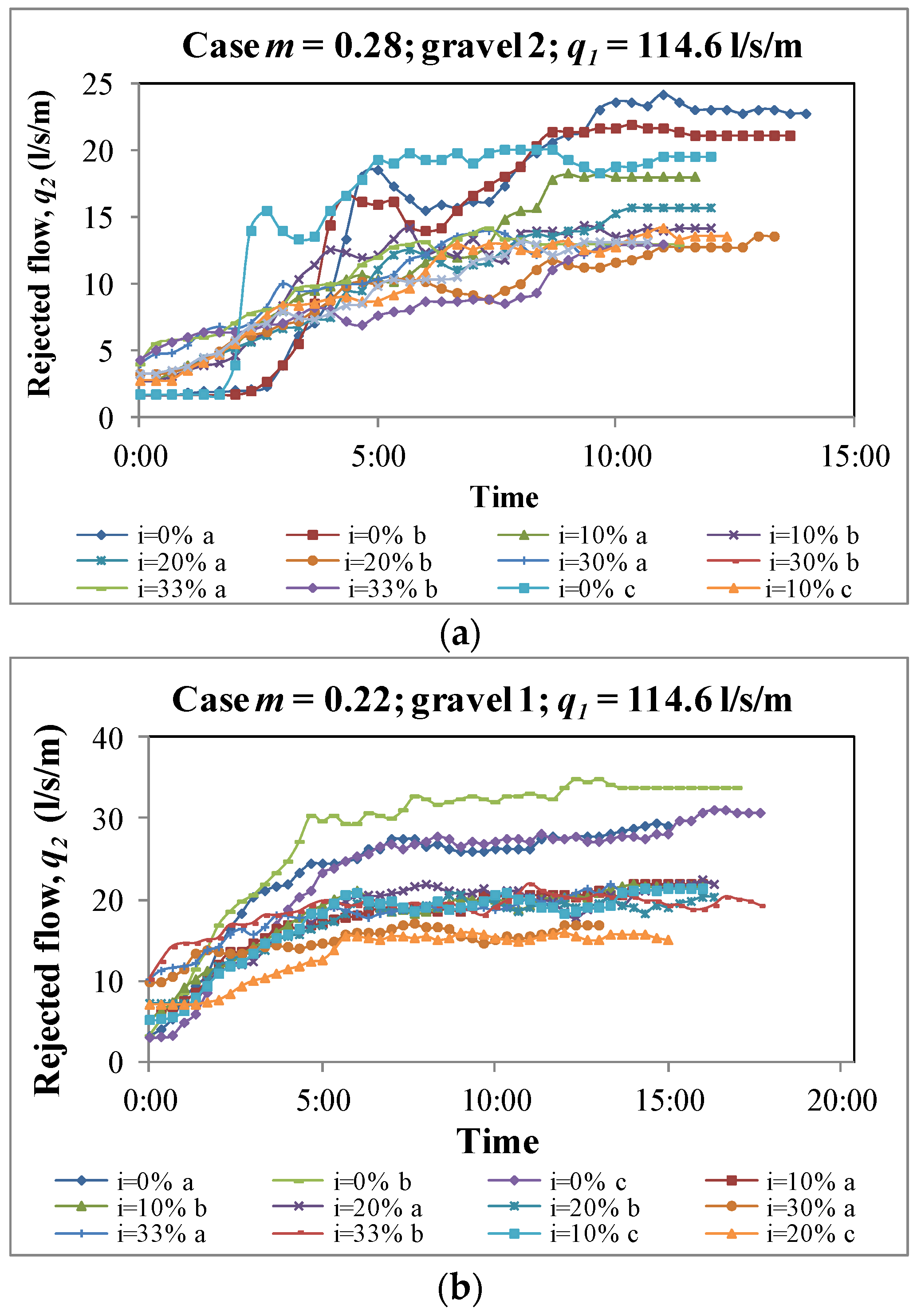
3.2. Sediment Tests
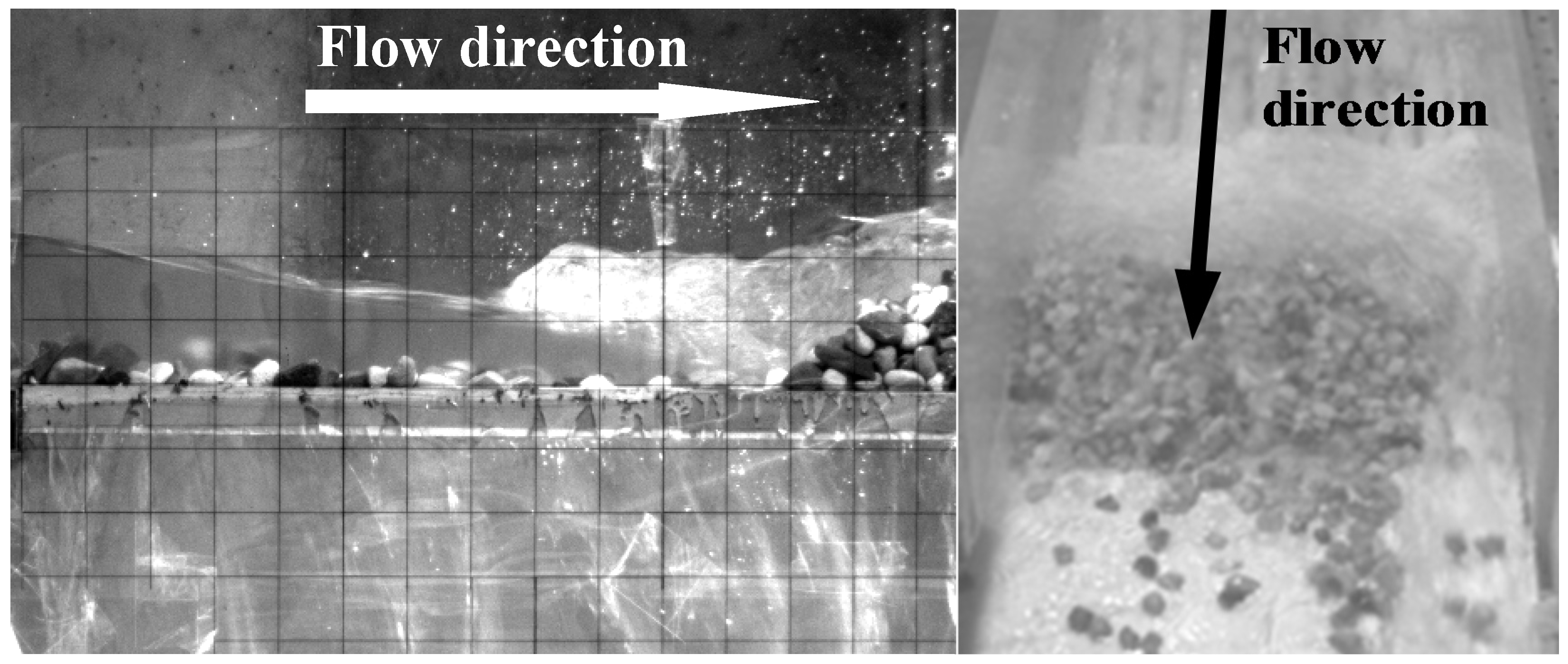
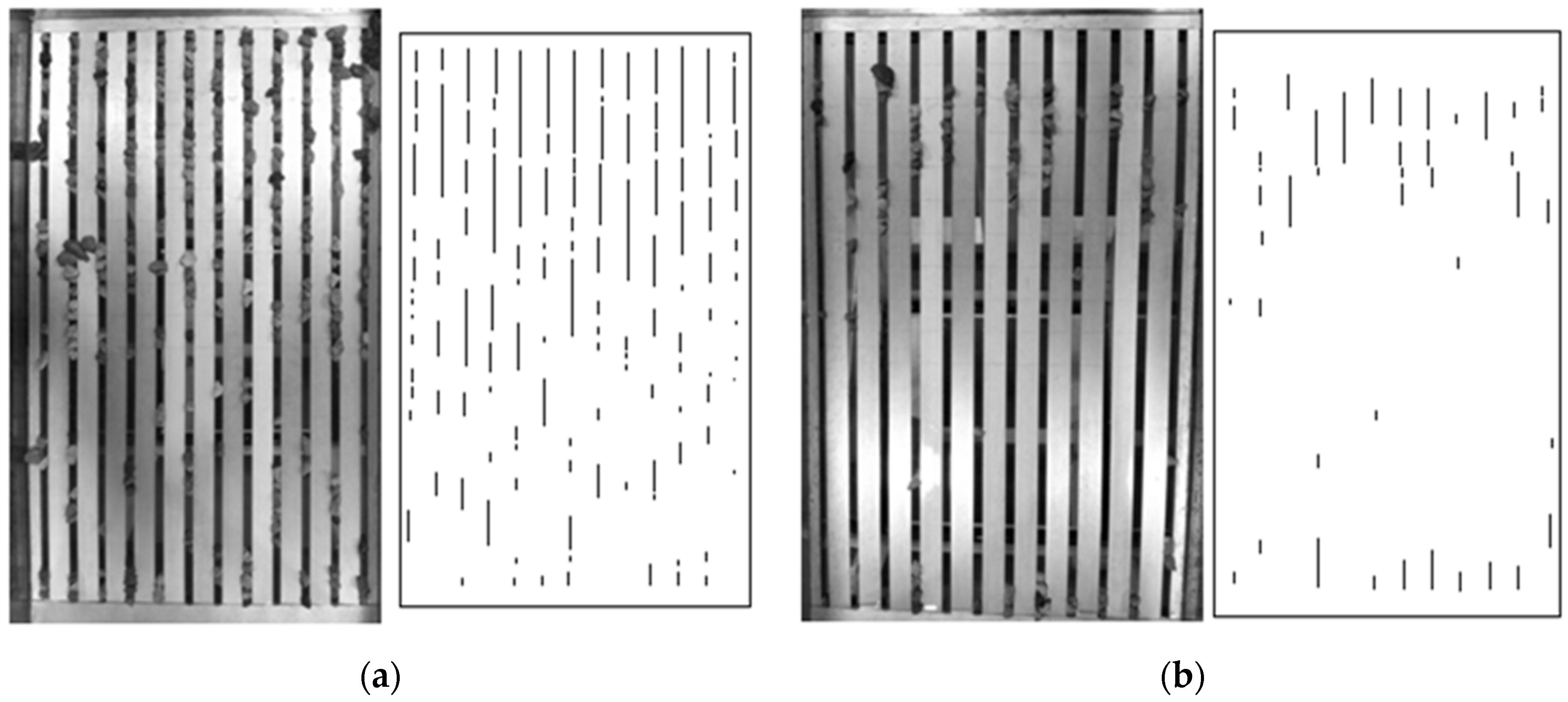
3.2.1. Deposition over the Racks
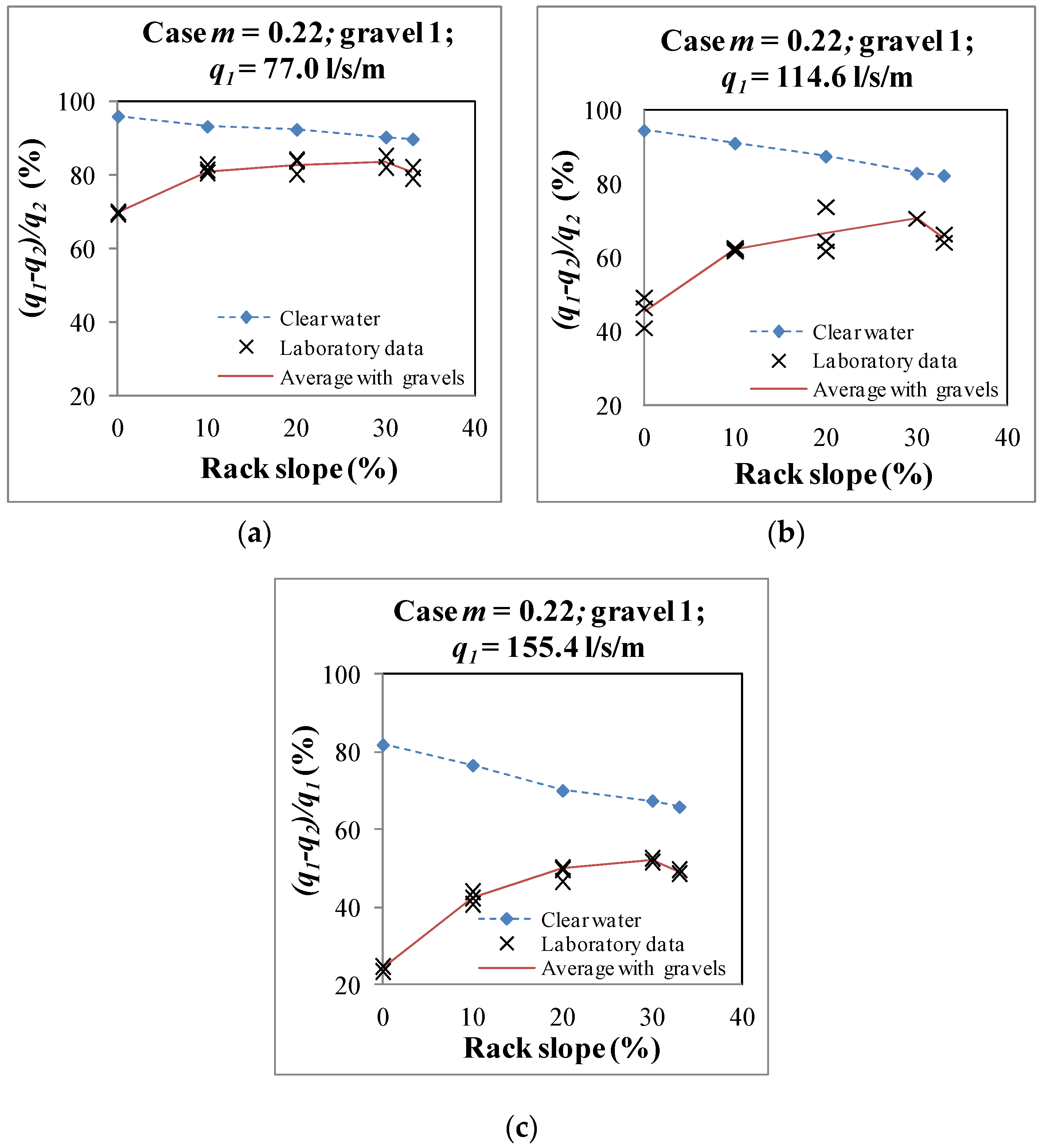
3.2.2. Efficiency of the Rack
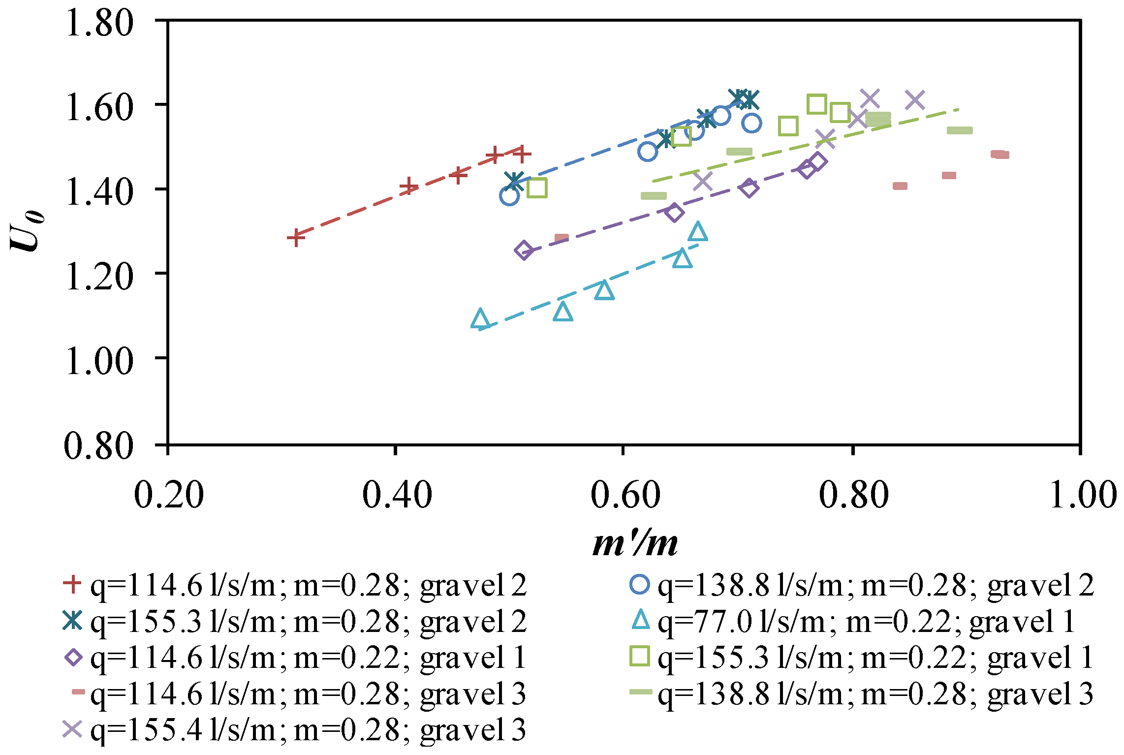
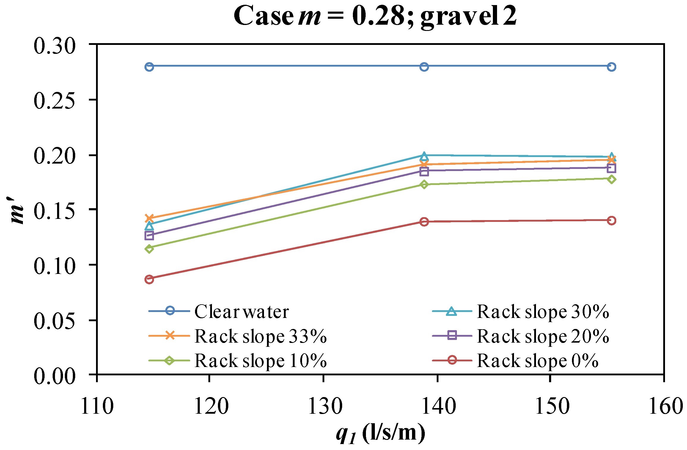
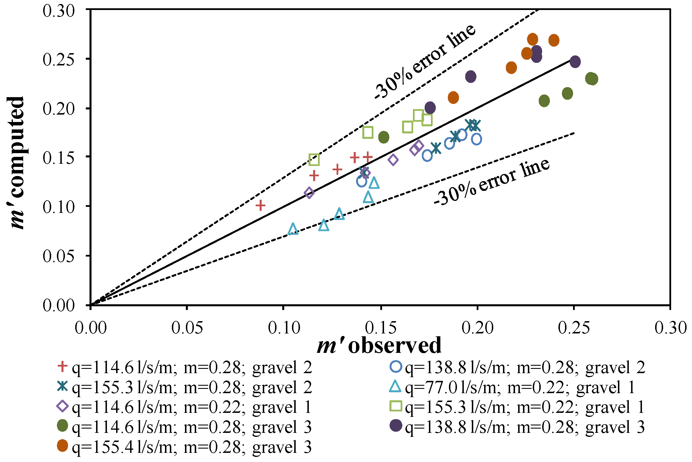
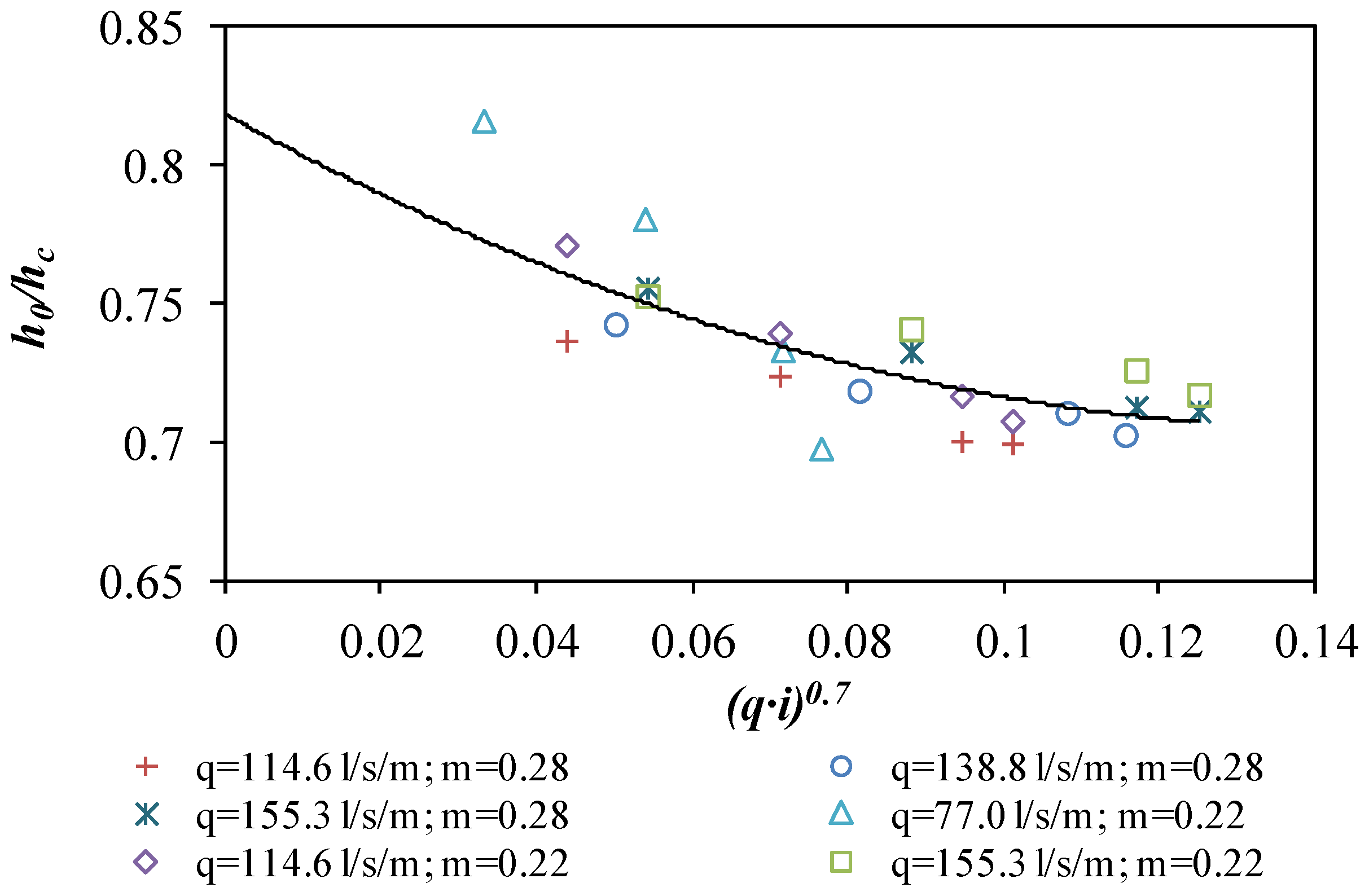
3.2.3. Effective Void Fraction
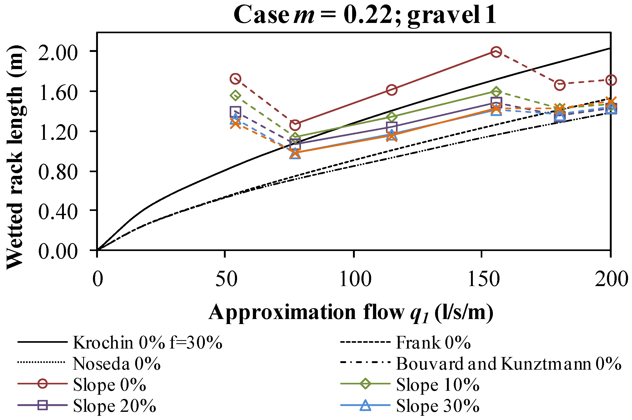
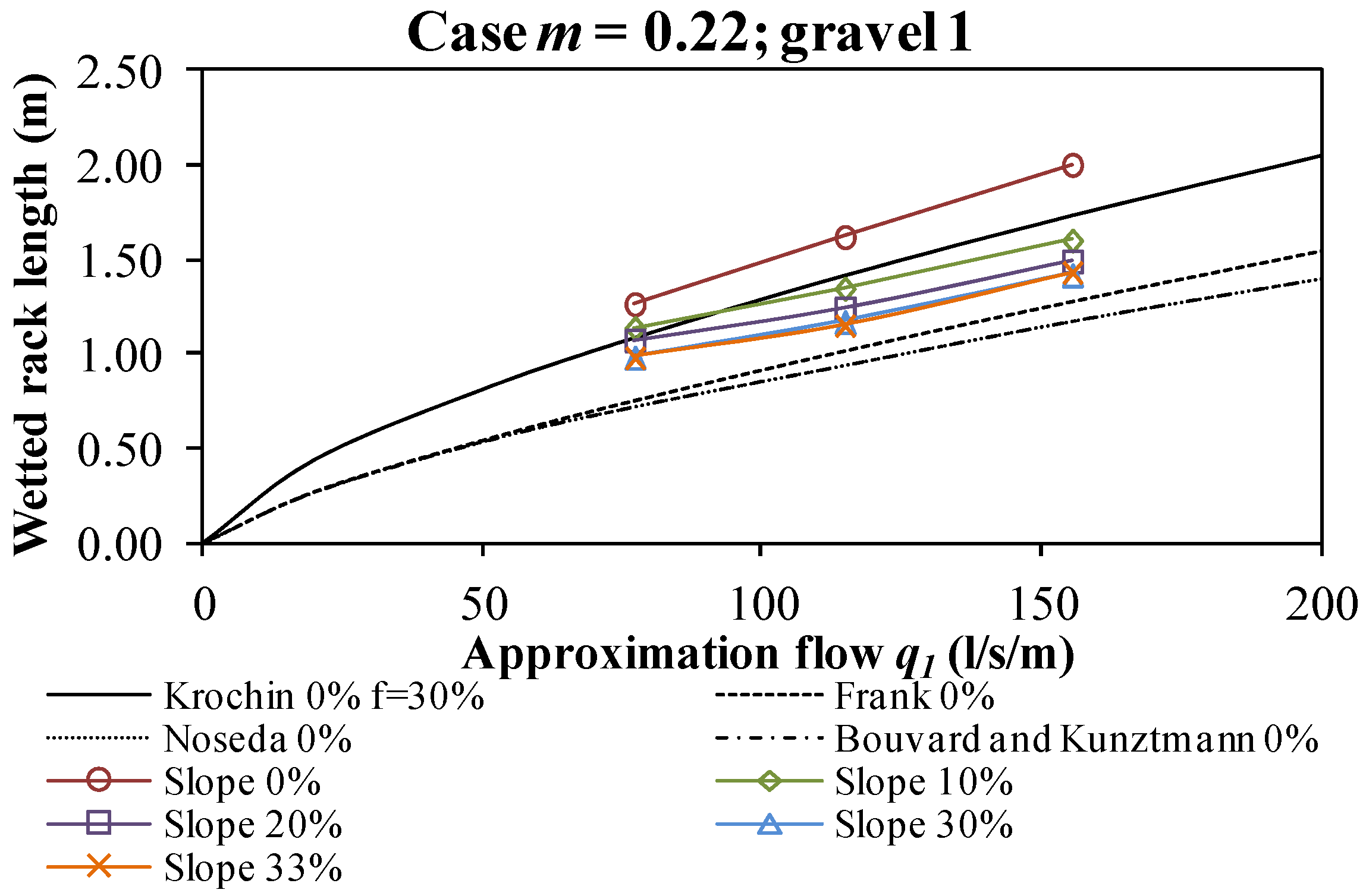
3.2.4. Effective Wetted Rack Length
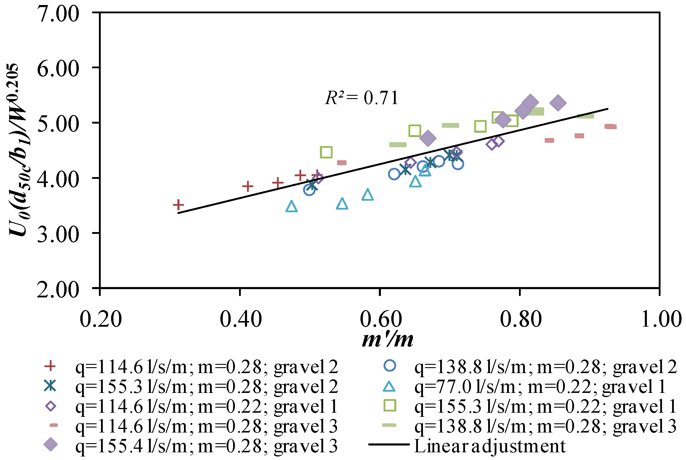
3.2.5. Relation between Occlusion and Hydraulic Parameters
4. Conclusions
Acknowledgments
Author Contributions
Conflicts of Interest
References
- Bouvard, M. Mobile Barrages & Intakes on Sediment Transporting Rivers; International Association of Hydraulic Engineering and Research (IAHR) Monograph: Rotterdam, The Netherlands, 1992. [Google Scholar]
- Raudkivi, A.J. Hydraulic Structures Design Manual; International Association of Hydraulic Engineering and Research (IAHR): Rotterdam, The Netherlands, 1993; pp. 92–105. [Google Scholar]
- Ract-Madoux, M.; Bouvard, M.; Molbert, J.; Zumstein, J. Quelques réalisations récentes de prises en-dessous à haute altitude en Savoie. La Houille Blanche 1955, 6, 852–878. [Google Scholar] [CrossRef]
- Simmler, H. Konstruktiver Wasserbau, Technische Universität Graz; Institut für Wasserwirtschaft und konstruktiven Wasserbau: Graz, Austria, 1978. [Google Scholar]
- Drobir, H. Entwurf von Wasserfassungen im Hochgebirge. Österr. Wasserwirtschaft 1981, 33, 243–253. [Google Scholar]
- Mostkow, M. Sur le calcul des grilles de prise d’eau. La Houille Blanche 1957, 4, 569–576. [Google Scholar] [CrossRef]
- Castillo, L.G.; Lima, P. Análisis del dimensionamiento de la longitud de reja en una captación de fondo. In Proceedings of the XXIV Congreso Latinoamericano de Hidráulica, Punta del Este, Uruguay, 21–25 November 2010.
- Conesa, C. La Acción Erosiva de las Aguas Superficiales en el Campo de Cartagena; Universidad de Murcia, Departamento de Geografía Física, humana y Análisis Regional: Murcia, Spain, 1989. [Google Scholar]
- Conesa, C. El Campo de Cartagena. Clima e Hidrología de un Medio Semiárido; Universidad de Murcia, Ayuntamiento de Cartagena, Comunidad de Regantes del Campo de Cartagena: Murcia, Spain, 1990. [Google Scholar]
- Navarro, F. El sistema Hidrográfico del Guadalentín; Consejería de Política Territorial, Obras Públicas y Medio Ambiente. Cuaderno Técnico No. 6: Murcia, Spain, 1991. [Google Scholar]
- Marín, M.D. Suficiencia Investigadora; Programa de Doctorado: Minería Medio Ambiente y Desarrollo Sostenible, Grupo I+D+i en Ingeniería Hidráulica y Medio Ambiente HIDR@M: Cartagena, Spain, 2011. [Google Scholar]
- Castillo, LG.; Marin, M.D. Hydrological and hydraulic characterization in semiarid zones. Analysis of model type, basin size and sediment transport formulae. In Proceedings of the International Conference on Fluvial Hydraulics, San Jose, Costa Rica, 5–7 September 2012.
- Garot, F. De Watervang met liggend rooster. Ing. Ned. Indie 1939, 7, 115–132. [Google Scholar]
- Noseda, G. Correnti permanenti con portata progressivamente decrescente, defluenti su griglie di fondo. L’Energia Elettrica 1956, 565–581. [Google Scholar]
- Righetti, M.; Lanzoni, S. Experimental study of the flow field over bottom intake racks. J. Hydraul. Eng. 2008, 134, 15–22. [Google Scholar] [CrossRef]
- Brunella, S.; Hager, W.; Minor, H. Hydraulics of bottom rack intake. J. Hydraul. Eng. 2003, 129, 2–10. [Google Scholar] [CrossRef]
- Bouvard, M. Debit d’une grille par en dessous. La Houille Blanche 1953, 2, 290–291. [Google Scholar] [CrossRef]
- Bouvard, M.; Kuntzmann, J. Étude théorique des grilles de prises d’eau du type “En dessous”. La Houille Blanche 1954, 5, 569–574. [Google Scholar]
- Frank, J. Hydraulische Untersuchungen für das Tiroler Wehr. Der Bauing. 1956, 31, 96–101. [Google Scholar]
- Frank, J. Fortschritte in der hydraulic des Sohlenrechens. Der Bauing. 1959, 34, 12–18. [Google Scholar]
- Krochin, S. Diseño hidráulico, 2nd ed.; Colección Escuela Politécnica Nacional: Quito, Ecuador, 1978. [Google Scholar]
- Orth, J.; Chardonnet, E.; Meynardi, G. Étude de grilles pour prises d’eau du type. La Houille Blanche 1954, 3, 343–351. [Google Scholar] [CrossRef]
- White, J.K.; Charlton, J.A.; Ramsay, C.A.W. On the design of bottom intakes for diverting stream flows. In Proceedings of the Institution of Civil Engineers; ICE Publishing: London, UK, 1972; Volume 51, pp. 337–345. [Google Scholar]
- Drobir, H.; Kienberger, V.; Krouzecky, N. The wetted rack length of the Tyrolean weir. In Proceedings of the 28th IAHR Congress, Graz, Austria, 22–27 August 1999.
- Ahmad, Z.; Kumar, S. Estimation of trapped sediment load into a trench weir. In Proceedings of the 11th International Symposium on River Sedimentation, University of Stellenbosch, South Africa, 6–9 September 2010; pp. 1–9.
- Castillo, L.G.; Carrillo, J.M.; García, J.T. Comparison of clear water flow and sediment flow through bottom racks using some lab measurements and CFD methodology. In WIT Transactions on Ecology and the Environment; Wessex Institute of Technology: New Forest, UK, 2013; Volume 172, pp. 227–237. [Google Scholar]
- Castillo, L.G.; Carrillo, J.M.; García, J.T. Flow and sediment transport through bottom racks. CFD application and verification with experimental measurements. In Proceedings of the 35th IAHR Congress, Chengdu, China, 8–13 September 2013.
- Castillo, L.G.; Carrillo, J.M.; García, J.T. Comparativa del flujo de agua limpia y con sedimentos a través de sistemas de captación de fondo utilizando datos de laboratorio y un modelo CFD. In Proceedings of the III Jornadas de Ingeniería del Agua, Valencia, Spain, 23–24 October 2013.
- ANSYS, Inc. ANSYS CFX-Solver Theory Guide, Release 13.0; ANSYS, Inc.: Canonsburg, PA, USA, 2010. [Google Scholar]
- Righetti, M.; Rigon, R.; Lanzoni, S. Indagine sperimentale del deflusso attraverso una griglia di fondo a barre longitudinali. In Proceedings of the XXVII Convegno di Idraulica e Costruzioni Idrauliche, Genoa, Italy, 12–15 September 2000; Volume 3, pp. 112–119.
- Castillo, L.G.; Carrillo, J.M. Numerical simulation and validation of intake systems with CFD methodology. In Proceedings of the 2nd IAHR European Congress, Munich, Germany, 27–29 June 2012.
- Castillo, L.G.; García, J.T.; Carrillo, J.M. Experimental measurements of flow and sediment transport through bottom racks. Influence of graves sizes on the rack. In Proceedings of the International Conference on Fluvial Hydraulics, Lausanne, Switzerland, 3–5 September 2014.
- Castillo, L.G.; García, J.T.; Carrillo, J.M. Intake systems in ephemeral rivers. In WIT Transactions on Ecology and the Environment; Wessex Institute of Technology: New Forest, UK, 2015; Volume 197, pp. 117–128. [Google Scholar]
- Montes, S. Hydraulics of Open Cannel Flow; American Society of Civil Engineers: Reston, VA, USA, 1998. [Google Scholar]
- Rouse, H. Fluid Hydraulics for Mechanics Engineers; Dover Publications: New York, NY, USA, 1938. [Google Scholar]


| Author | Formulation |
|---|---|
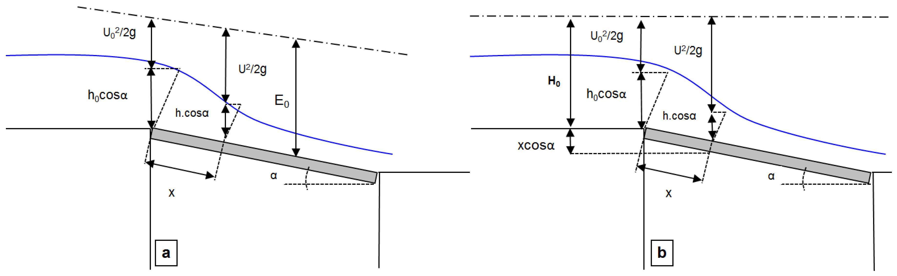
| Noseda [14] | E0 = specific energy head at the beginning of the rack |
| Bouvard and Kunztmann [18] | h1 = flow depth at the beginning of the rack; hc = critical depth; m″ = product of void ratio and discharge coefficient |
| Frank [19,20] | h1 = flow depth at the beginning of the rack; q1 = specific approximation flow; α = angle of rack with horizontal |
| Krochin [21] | q1 = specific approximation flow; f = obstruction coefficient |
| A | B | C | ||
|---|---|---|---|---|
| Space between bars b1 (mm) | 5.70 | 8.50 | 11.70 | |
| Void ratio | 0.16 | 0.22 | 0.28 | |
© 2016 by the authors; licensee MDPI, Basel, Switzerland. This article is an open access article distributed under the terms and conditions of the Creative Commons Attribution (CC-BY) license (http://creativecommons.org/licenses/by/4.0/).
Share and Cite
Castillo, L.G.; García, J.T.; Carrillo, J.M. Experimental and Numerical Study of Bottom Rack Occlusion by Flow with Gravel-Sized Sediment. Application to Ephemeral Streams in Semi-Arid Regions. Water 2016, 8, 166. https://doi.org/10.3390/w8040166
Castillo LG, García JT, Carrillo JM. Experimental and Numerical Study of Bottom Rack Occlusion by Flow with Gravel-Sized Sediment. Application to Ephemeral Streams in Semi-Arid Regions. Water. 2016; 8(4):166. https://doi.org/10.3390/w8040166
Chicago/Turabian StyleCastillo, Luis G., Juan T. García, and José M. Carrillo. 2016. "Experimental and Numerical Study of Bottom Rack Occlusion by Flow with Gravel-Sized Sediment. Application to Ephemeral Streams in Semi-Arid Regions" Water 8, no. 4: 166. https://doi.org/10.3390/w8040166