Development of Ecogeomorphological (EGM) Stream Design and Assessment Tools for the Piedmont of Alabama, USA

Abstract

Regional data needed for effective stream restoration include hydraulic geometry relationships (i.e., regional curves) and reference channel morphology parameters. Increasingly ecological conditions are being considered when designing, implementing, and assessing restoration efforts. We provide morphology relationships and associated ecological endpoint curves for reference streams in the Alabama piedmont. Twenty-one reference stream reaches were identified in the Tallapoosa drainage of Alabama, ranging from 0.2 to 242 km² drainage area. Geomorphic surveys were conducted in each stream to measure riffle cross-sections and longitudinal profiles and related to drainage area to develop regional curves. Fish, crayfish, and benthic macroinvertebrates were collected from each surveyed reach and related to drainage area and geomorphic data to provide associated biological community endpoints. Bankfull channel cross-section area, width, mean depth, and estimated discharge were strongly correlated to watershed drainage area, similar to efforts in other areas of the Piedmont ecoregion. Multiple measures of fish assemblages and crayfish size were strongly predicted by drainage area and geomorphic dimensions. Macroinvertebrates showed no taxonomic and limited functional relationships with drainage area and geomorphic dimension. These tools, which integrate geomorphological and ecological conditions, can result in improved stream evaluations and designs increasing the effectiveness of stream restoration projects.

1. Introduction

Stream restoration efforts are increasingly popular approaches to offset the physical and biological effects associated with anthropogenic degradation [1]. These efforts are often focused on returning systems to some approximation of an ideal or natural trajectory and are the foundation for the growing compensatory stream mitigation industry [2]. The cornerstone of most stream restoration projects generally is the physical manipulation of channel shape and pattern in an attempt to reduce erosion and re-establish or enhance habitats, ecological condition, and function. Thus the ability to accurately identify idealized and realized physical, biological and ecological conditions is a critical factor when assessing the need and setting the goals and objectives of restoration projects. Of particular importance is establishing the linkages between physical manipulation (“inputs”) and ecological response (“outcomes”) when designing and assessing restoration efforts [3], however these linkages are dynamic and require extensive field data collection to determine [2,4].

Stream channel hydraulic geometry theory describes the relationships between channel dimensions (e.g., cross-section area, width, depth) and stream discharge [5] or drainage area [6]. Specifically, bankfull discharge is considered to represent the approximate channel forming flow, thus identifying the bankfull channel dimensions and associated floodplain configuration is the basis for restoration design [7]. These hydraulic geometry relationships vary by physiographic region as they are influenced by geology, hydrology, soil, vegetation, and climate. Thus hydraulic geometry relationships across multiple streams of various sizes within a physiographic region are known as regional curves [6]. Regional curves are typically one-variable regressions relating bankfull dimensions, geometry, and discharge to drainage area described by power-functions and are the fundamental tool used by engineers to estimate these parameters for natural channel stream restoration designs. Although national curves exist and are used in some situations (e.g., Soil and Water Assessment Tool (SWAT), [8]), increasing data show that regional curves based on physiographic provinces and smaller regions are more predictive than a broad-scale nationwide curve, and that finer-scale curves derived within a physiographic province are even more reliable [9].

Restoration efforts have involved a strong focus on the physical condition of the stream channel with the assumption that biological and functional recovery will follow in suit to various degrees of success [10]. Natural channel design approaches specifically focus on matching the re-configured pattern, profile, and dimension of stream channels to local reference conditions [11,12]. Increasing focus is shifting towards considering specific biological and ecological conditions, processes and dynamics in association with channel geomorphology [13,14,15]. Some studies have shown strong relationships between stream geomorphology and biotic assemblages and/or ecological integrity [15,16], whereas others have demonstrated weak concordance between geomorphology and biodiversity, presumably due to functional redundancy [17]. Understanding the nature of the foundational relationships between ecological parameters and geomorphology, and how these vary across the landscape, are particularly important when assessing need, designing, and evaluating success of stream restoration projects [18].

The southeastern US has been the target of extensive land use change, highlighted by intense agricultural expansion in late 1800s and early 1900s, agricultural abandonment and reforestation through the 20th century, and more recent urban development [19,20]. The southeast in general, and the Piedmont ecoregion in particular, has been subject to pervasive forest conversion with subsequent erosion and sediment deposition in receiving waters, with some river systems reporting up to 6 m of deposition [21,22]. The southeastern United States is also a global biodiversity hotspot for aquatic fauna, particularly fishes, aquatic reptiles and amphibians, mollusks, crayfishes and many insect groups, often due to the preponderance of endemism in the region [22]. As a result of dramatic land cover disturbance and extremely high biotic diversity, aquatic systems in the southeastern United States also have experienced some of the most extensive ecosystem and species losses in North America and globally [23,24]. Not surprisingly, considerable work has targeted restoration of Piedmont streams, with many regional curves developed for the Piedmont Physiographic Region across southeastern states, including Georgia, North Carolina, Virginia, Maryland and Pennsylvania [3,7,25,26]. Prior to this study, no regional curves were available for the Piedmont Physiographic Region of Alabama, and none of the existing curves have associated biological endpoints. This is particularly critical given the unparalleled level of aquatic biodiversity in the state and ecoregion [27]. Thus the objectives of this effort were to develop ecogeomorphological design and assessment tools for the Alabama Piedmont in the form of regional curves for bankfull hydraulic geometry and aquatic biota, with the anticipation that these tools would be of broader contextual use in other portions of the Piedmont or other ecoregions entirely.

2. Methods

2.1. Reference Reach Selection

Study streams were located in the Tallapoosa River drainage in the Piedmont ecoregion of eastern Alabama (Figure 1). We confined study sites to one drainage to control for drainage-specific taxonomic variation in crayfishes and fishes. All streams were selected through team-based field reconnaissance and only unanimously-determined reference alluvial reaches were used. Individual team members (i.e., authors) had extensive experience and expertise in geomorphology, plant ecology, soil science, and aquatic ecology in the Piedmont ecoregion. All reference reaches were well-connected to alluvial floodplains indicated by recent deposition (fresh sand deposits in floodplain) and no evidence of incision (bank height ratios less than 1.2). Further, all reaches had freely-formed meander patterns with alternating riffle and pool bedforms, were unconfined for a longitudinal length of at least 20 times bankfull width, and were considered stable channels based on observed substrate composition (e.g., high proportion of gravel and cobble, low proportion of shifting sand). All streambanks and floodplains were well-vegetated with little evidence of erosion or invasive species, and were contained within heavily-forested rural watersheds (% impervious surface ranged from 0.01%–5.82%). Twenty-one streams were chosen to represent a range of drainage areas across the region. All streams were perennial with the exception of two in the smallest watersheds (

Table 1. Drainage area (DA), percent impervious surface (%IS), slope, bankfull dimensions, bankfull discharge parameters and Rosgen classification [11] for 21 reference streams of the Tallapoosa basin in the Piedmont of east Alabama. “UT” referes to “unnamed tributary”, see text for variable definitions. %IS determined from the 2011 National Land Cover Database [41].

Site Name	DA (km2)	%IS	Slope (m/m)	Abkf (m2)	Wbkf (m)	Wfpa (m)	dbkf (m)	Wbkf/dbkf	Wfp/Wbkf	Manning’s n	Rh (m)	Vbkf (m/s)	Qbkf (m3/s)	Rosgen
UT Chewacla Creek	0.2	0.86	0.0067	0.4	3.0	13	0.1	25	4.3	0.046	0.1	0.5	0.2	C
UT Moores Mill Creek	0.4	2.06	0.0101	0.8	2.4	8	0.3	7.9	3.3	0.046	0.3	0.9	0.8	E
UT Coon Creek	0.4	0.14	0.0125	1.1	3.7	33	0.3	12.3	8.8	0.048	0.3	1.0	1.2	C
Pate Spring	0.5	0.72	0.0081	0.8	2.6	20	0.3	8.6	7.6	0.046	0.3	0.8	0.7	E
Waterfall Creek	0.7	0.32	0.0133	1.0	4.4	18	0.2	20.4	4.1	0.040	0.2	1.0	1.2	C
Clara’s Creek	0.8	0.01	0.0085	1.5	3.9	10	0.4	10.2	2.8	0.040	0.3	1.1	1.9	E
Patterson Creek	0.8	0.36	0.0094	1.4	3.9	23	0.4	10.8	5.8	0.046	0.3	1.0	1.7	E
UT Ropes Creek	0.9	0.14	0.0062	0.9	3.4	50	0.2	14	14.6	0.046	0.2	0.7	0.6	C
Loombeam Spring	1.3	0.09	0.0105	0.8	3.7	35	0.2	15	9.6	0.042	0.2	0.9	0.8	C
UT Wesobulga Creek	2.0	0.29	0.0092	1.3	4.1	35	0.3	12.4	8.6	0.047	0.3	0.9	1.4	C
UT Emuckfaw Creek	2.5	0.15	0.0080	1.7	4.7	8.4	0.4	12.9	1.8	0.046	0.3	0.9	1.8	Bc
Pile Creek	6.1	0.14	0.0046	3.3	7.3	50	0.5	16	6.8	0.053	0.4	0.7	2.7	C
Osborn Creek	7.5	0.50	0.0030	3.3	7.0	60	0.5	14.9	8.6	0.048	0.4	0.7	2.5	C
Ropes Creek	7.8	0.16	0.0045	6.7	8.1	86	0.8	9.8	10.6	0.052	0.7	1.1	8.1	E
Coon Creek	8.8	0.95	0.0020	5.8	11.3	30	0.5	21.8	2.7	0.040	0.5	0.7	4.7	C
Jones Creek	12.2	0.40	0.0031	7.7	8.5	47	0.9	9.3	5.5	0.040	0.8	1.2	10.7	E
UT Hillabee Creek	38.6	0.20	0.0036	11.4	11.0	80	1.0	10.6	7.3	0.035	0.9	1.6	21.6	E
Choctafaula Creek	53.1	3.26	0.0014	14.7	13.8	43	1.1	12.9	3.1	0.039	1.0	1.0	16.3	C
Little Hillabee Creek	54.6	0.18	0.0029	16.1	13.8	52	1.2	11.9	3.8	0.035	1.1	1.6	30.0	E
Chewacla Creek	118.9	5.82	0.0046	25.1	26.2	33	1.0	27.3	1.3	0.035	1.0	1.9	54.7	Bc
Enitachopco Creek	242.1	0.45	0.0012	60.0	26.4	48	2.3	11.5	1.8	0.040	2.1	1.4	97.7	Bc

). At each stream, a representative reach was selected at least 100 m upstream or downstream of the nearest road crossing to minimize any potential bridge effects when applicable. Reach lengths were at least 20× bankfull width, with a minimum of 150 m and maximum of 300 m, and were selected to contain most available physical structures and habitats in the stream [28,29].

2.2. Stream Geomorphology

Reference streams were classified using the Rosgen stream classification system [11] and surveyed using total station survey equipment and hand-held computer to measure riffle cross-sections and longitudinal profiles [30]. Cross-sections were located at stable riffle features near indicators of the active floodplain, generally with three cross-sections per stream. For each cross-sectional profile, points reflecting breaks in slope between the right and left bank were recorded. For longitudinal profiles, points along the channel thalweg, water surface, and top of bank were recorded at the start and end of observed bed features and other breaks in slope [31]. Longitudinal profiles were initiated and terminated at the head of a riffle. For each site, the following bankfull channel dimensions were quantified to derive baseline geomorphic regional rating curves: drainage area (DA), estimated bankfull discharge (Q_bkf), bankfull channel cross-section area (A_bkf), bankfull channel width (W_bkf), bankfull channel mean depth (d_bkf), width-to-depth ratio (W_bkf/d_bkf), and entrenchment ratio (W_fpa/W_bkf) where W_fpa is the width of the flood-prone area.. Additionally, in the 15 smallest watersheds, bedform dimension and slope variables were quantified, which included riffle length, riffle length/W_bkf, pool length, pool length/W_bkf, pool spacing, pool spacing/W_bkf, riffle slope, and riffle slope/reach slope [6]. To estimate bankfull discharge for each stream, the Manning equation was applied using estimates for roughness (Manning n) based on the Cowan method [32].

To compare these curves to other Piedmont curves generated from previous efforts, we developed individual general linear models for each cross-section profile dependent variable (Q_bkf, A_bkf, W_bkf, and d_bkf) for Alabama and a given eastern US state. For each model developed, drainage area, data source, and drainage area*data source interaction were the predictor variables, with all empirical data being log transformed prior to analysis [33]. Outside data sources included regional curves from Georgia [34], North Carolina [35], Virginia [26], Maryland [25], and Pennsylvania [7]. A significant interaction between drainage area and data source denoted regression slope difference, thus differences in regional curves [36].

2.3. Ecological Endpoints

Aquatic biota and their habitats were quantified from the surveyed reach in 16 of the reference streams during May–June 2011 to serve as ecological endpoints associated with geomorphic regional curves. Fishes and crayfishes were collected with a backpack electroshocker and seines from all represented habitats within the reach [28]. The entire reach was sampled for fishes with a single pass, and the first third of the reach was sampled for crayfishes with a triple pass. A team of three people, with one person using the electroshocker and two people collecting stunned animals with dip nets, worked habitats in an upstream fashion. Catch-per-unit-effort (CPUE) was measured as fish collected over area of habitat sampled (fish/m²), and all subsequent assemblage metrics (besides taxa richness) were based on CPUE values. All crayfish and fish were identified to species, measured, and sexed (crayfish only). Functional feeding and breeding groups for fish were assigned according to FishTraits database [37].

We collected benthic macroinvertebrates with a Surber sampler (0.09 m², 250 μm mesh) in 3 separate representative riffle habitats in the reach [28] by consolidating three collections in each habitat resulting in a 0.27 m² sample from each riffle. We characterized stream microhabitat when macroinvertebrates were sampled by quantifying mean depth, current velocity (Marsh-McBirney model 2000 flow meter) and visually estimating percent benthic substrate composition for each point of collection. Upon collection, we elutriated excess sediment with a 500 μm mesh sieve, and preserved organisms in 95% ethanol in the field for transport to the lab. Macroinvertebrates were subsampled with a random grid sorting tray until >300 organisms were picked by hand under a dissecting scope [38]. After subsampling, we searched the remaining sample and noted the presence of large organisms in the whole sample not represented in subsamples [39]. All macroinvertebrates were measured and identified to genus except Chironomidae, which were identified to Tribe, and subsequently assigned to functional feeding groups [40].

At each collection reach, physical habitat was recorded when animals were sampled. Ten cross-sectional transects were established along the reach and depth, flow, and width were determined at three equidistant points along each transect. At the downstream end of the reach, pH (Sharp pH52 meter, Milwaukee Instruments, Inc., Rocky Mount, NC, USA), conductivity (C66 Sharp meter, Milwaukee Instruments, Inc., Rocky Mount, NC, USA), dissolved oxygen and stream temperature (YSI 55 meter), and stream discharge (Marsh-McBirney Flo-Mate 2000, Hach, Loveland, CO, USA) were recorded. Calculated biotic metrics (total catch, catch per unit area, species richness/diversity, and assemblage proportions) were correlated with local habitat measures and fitted against reach-scale geomorphological assessments. In contrast to the power models describing bankfull dimensions and drainage area relationships, fish assemblage and bankfull dimensions relationships are described by the logarithmic model:

Fish response = y_o + a ln x

(1)

where y_o is the y-intercept, a is the slope, and x is bankfull measurement. This model accounts for the generally rapid biotic changes observed with moving from small headwaters to medium-sized streams. Due to their smaller regional taxonomic pool (n = 8), crayfish relationships are described by power models, similar to bankfull dimensions/drainage area relationships. All non-normal data were appropriately transformed prior to correlation or regression analyses.

3. Results

3.1. Bankfull Channel Dimensions

Twenty-one reference streams with drainage areas ranging from 0.2 to 242.1 km² were surveyed for regional geomorphic rating curves. Reach slope ranged from 0.0012 m/m to 0.0133 m/m, W_bkf ranged from 2.4 m to 26.4 m, mean d_bkf ranged from 0.1 m to 2.3 m, and A_bkf 0.4 to 60.0 m² (Table 1). There was considerable range in Q_bkf as evidenced by the variation in stream size and shape, with Q_bkf estimates ranging from 0.2 m³/s to 97.7 m³/s (Table 1). These four descriptors of hydraulic geometry were plotted independently against drainage area with a high degree of predictability to create regional curves (Figure 2). The regression equations for these are summarized with the following power functions:

A_bkf = 1.21 DA ^0.653 (R² = 0.959)

(2)

W_bkf = 3.96 DA ^0.335 (R² = 0.944)

(3)

d_bkf = 0.305 DA ^0.319 (R² = 0.867)

(4)

Q_bkf = 1.17 DA ^0.757 (R² = 0.922)

(5)

Width/depth ratios (W_bkf/d_bkf) ranged from less than 12 for the narrow, deep streams to greater than 20 for the wide and shallow streams. W_fpa ranged from 8–86 m and entrenchment ratios (W_fpa/W_bkf) ranged from 1.3–14.6 (Table 1).

3.2. Bedform Dimensions

Fifteen reference streams with drainage areas ranging from 0.2 to 12.2 km² were surveyed for bedform dimensions and slope. Mean riffle length ranged from 1.6–18.9 m, riffle length/W_bkf ranged from 0.6–2.2, mean pool length ranged from 5.1–28.4 m, pool length/W_bkf ranged from 1.5–5.5 (

Table 2. Bedform dimensions for 15 reference streams of the Tallapoosa basin in the Piedmont of east Alabama. See text for variable definitions.

Site Name	Riffle Length (m)	Riffle Length/Wbkf	Pool Length (m)	Pool Length/Wbkf	Riffle/Reach Length	Pool Spacing (m)	Pool Spacing/Wbkf	Riffle Slope (m/m)	Riffle/Reach Slope
UT Chewacla Creek	6.6	2.2	5.1	1.7	0.60	11.7	3.5	0.0116	1.7
UT Moores Mill Creek	3.7	1.5	13.4	5.5	0.25	15.2	6.3	0.0325	3.2
Pate Spring	1.6	0.6	9.5	3.6	0.14	12.1	4.6	0.0564	7.0
Waterfall Creek	6.7	1.5	10.0	2.3	0.40	15.0	3.4	0.0419	3.1
Clara’s Creek	3.5	0.9	13.0	3.3	0.27	13.6	3.5	0.0416	4.9
Patterson Creek	4.5	1.1	8.6	2.2	0.34	13.1	3.3	0.0300	3.2
UT Ropes Creek	4.8	1.4	6.6	1.9	0.42	11.2	3.3	0.0129	2.1
Loombeam Spring	6.5	1.8	16.8	4.6	0.34	18.2	5.0	0.0343	3.3
UT Wesobulga Creek	5.3	1.3	9.7	2.4	0.41	12.6	3.1	0.0261	2.8
UT Emuckfaw Creek	5.9	1.3	11.4	2.4	0.34	15.1	3.2	0.0208	2.6
Pile Creek	6.7	0.9	16.7	2.3	0.29	24.9	3.4	0.0177	3.8
Osborn Creek	5.7	0.8	24.1	3.5	0.24	25.6	3.7	0.0162	5.4
Ropes Creek	10.7	1.3	11.9	1.5	0.55	11.2	1.4	0.0175	3.9
Coon Creek	9.1	0.8	26.2	2.3	0.26	41.0	3.6	0.0071	3.5
Jones Creek	18.9	2.2	28.4	2.6	0.57	-	-	0.0090	2.9

). Both riffle length and pool length were positively related to DA, with pools generally being about twice as long as corresponding riffles (Figure 3). Riffle length ratios and pool length ratios were not related to drainage area. Mean pool spacing ranged from 11.2–41.0 m and pool spacing/W_bkf ranged from 1.4–6.3 (Table 2), however neither were related to drainage area. Mean riffle slope ranged from 0.0071–0.0564 and riffle /reach slope ranged from 1.7–7.0 (Table 2). Both were positively related to drainage area, with riffle slopes being approximately 3x the reach slope (Figure 3).

3.3. State Comparisons

Alabama Piedmont regional curves derived in this study showed considerable similarity to Piedmont regional curves generated from other states (Figure 4). There was no significant interaction between Alabama and Georgia, Maryland, or North Carolina any of the bankfull cross-section profile variables (

Table 3. Results from separate ANCOVAs to compare Alabama Piedmont regional curves to Piedmont regional curves from other states. Values are p-values (significant values in bold) from the interaction term in a linear model assessing drainage area, data source, and drainage area*data source on channel dimension variables. Source data for comparisons include Georgia [32], North Carolina [33], Virginia [24], Maryland [23], and Pennsylvania [7].

Regional Curve	Abkf	Wbkf	Dbkf	Qbkf
Alabama vs. Georgia	0.268	0.069	0.96	0.655
Alabama vs. Maryland	0.141	0.197	0.603	0.993
Alabama vs. North Carolina	0.778	0.549	0.486	0.602
Alabama vs. Pennsylvania	0.052	0.036	0.789	0.418
Alabama vs. Virginia	0.012	0.017	0.213	0.038

). There were significant difference in the slopes of Alabama and Pennsylvania models of A_bkf and W_bkf, with slope for Pennsylvania being steeper. No significant differences were observed for d_bkf and Q_bkf between Alabama and Pennsylvania. There were also differences between Alabama and Virginia models for A_bkf, W_bkf, and Q_bkf, but not D_bkf. As in comparisons with Pennsylvania, the slopes of models derived from Virginia were steeper than models derived from Alabama (Figure 4).

3.4. Fish Response

Physicochemical conditions at the time of sampling were typical of early summer conditions in the region (

Table 4. Streams sampled for biotic assemblages and associated mean physicochemical conditions at time of sampling.

Site Name	Drainage Area (km2)	Width (m)	Maximum Depth (m)	Flow Velocity (m/s)	Discharge (m3s)	pH	Conductivity (μS)	Dissolved Oxygen (mg/L)	Temperature (°C)
UT Coon Creek	0.4	1.4	0.2	0	0.001	7.1	50.4	4.4	15.5
Pate Spring	0.5	1.1	7.0	0.1	0.001	6.4	15.4	7.2	13.4
Waterfall Creek	0.7	1.3	0.3	0.3	0.001	6.9	58.0	7.7	17.5
Clara’s Creek	0.8	1.8	0.3	0	0.002	7.4	47.0	7.6	21.3
Patterson Creek	0.8	1.7	1.5	0.1	0.005	6.9	38.3	8.6	17.9
Loombean Spring	1.3	1.5	0.4	0.1	0.004	6.6	36.0	8.3	15.0
UT Wesobulga Creek	2.0	1.3	0.5	0.1	0.005	6.7	11.0	9.7	11.8
UT Emuckfaw Creek	2.5	2.3	0.4	0.2	0.005	7.2	38.4	8.6	13.4
Pile Creek	6.1	2.7	0.6	0.5	0.029	6.7	12.3	9.5	13.9
Osborn Creek	7.5	3.5	0.7	0.3	0.013	7.1	14.3	9.5	14.2
Ropes Creek	7.8	2.0	0.3	0.2	0.023	7.3	45.5	9.3	14.2
Coon Creek	8.8	2.4	0.4	0.2	0.007	7.1	58.1	8.0	19.9
Jones Creek	12.2	3.2	0.3	0.6	0.053	6.9	18.5	9.5	14.3
Little Hillabee Creek	38.6	5.8	1.1	0.4	0.091	6.7	42.9	7.3	24.6
Chewacla Creek	118.9	4.3	1.6	0.3	0.023	7.5	184.5	8.1	21.3
Enitachopco Creek	242.1	8.2	1.3	0.1	0.050	7.0	39.0	6.8	25.5

). A total of 4858 fish specimens comprising 10 families and 51 species were collected in the reference reaches (Table S1). Across all streams, Cyprinidae was the most taxa rich (16 spp.) followed by Centrarchidae (10 spp.), Percidae (8 spp.), Catastomidae (6 spp.), Ictaluridae (4 spp.), Cottidae (2 spp.), and Fundulidae (2 spp.), with Anguillidae, Petromyzontidae, and Poecilidae being represented by one species each (Table S1).

Total fish catch ranged from 35 to 959 individuals per stream, CPUE ranged from 0.95 to 16.94 fish/m², species richness ranged from 1 to 27, and species diversity (Shannon’s H’) ranged from 0 to 2.5 (

Table 5. Total catch, catch-per-unit-effort (CPUE) (fish/m²), species richness (Richness), diversity (Shannon’s H’), and percent of fish assemblage as different breeding guilds (%C, %G, and %L), range distribution categories (%E, %NE, and %WS), and feeding guilds (%H, %I, %O, and %P). See text for explanations of abbreviations.

Stream Name	Catch	CPUE	Richness	Diversity	%C	%G	%L	%E	%NE	%WS	%H	%I	%O	%P
UT Coon Creek	35	0.95	4	0.3	0	94	6	0	5	95	0	3	94	3
Pate Rd Spring	73	2.07	1	0	0	100	0	0	0	100	0	0	100	0
Waterfall Creek	136	1.48	2	0	0	100	0	0	0	100	0	1	99	0
Clara’s Creek	117	2.09	2	0.5	0	100	0	0	0	100	0	0	82	18
Patterson Creek	165	3.03	6	1.4	2	55	43	0	45	55	0	19	28	53
Loombean Spring	177	3.05	11	1.9	5	49	46	0	29	71	1	51	32	15
UT Wesobulga Creek	101	2.27	11	1.3	1	66	33	0	31	69	1	12	59	28
UT Emuckfaw Creek	344	7.06	15	2.2	3	38	58	0	17	83	2	65	13	20
Pile Creek	166	3.96	12	2.2	11	28	60	0	39	61	1	76	7	16
Osborn Creek	286	4.84	13	2.3	6	34	61	0	42	58	5	83	2	10
Ropes Creek	130	2.06	10	1.8	23	50	27	0	33	67	0	90	2	8
Coon Creek	835	11.9	21	2.1	0	19	81	1	4	95	2	95	1	2
Jones Creek	173	3.89	19	2.5	36	26	38	7	46	47	4	85	7	4
Little Hillabee Creek	212	4.89	22	2.5	25	49	22	8	36	57	0	92	6	2
Chewacla Creek	959	16.4	27	2.2	35	46	19	8	0	92	22	71	0	7
Enitachopco Creek	949	12.5	25	2.2	34	23	43	19	55	26	2	89	1	8

). The percent of the fish assemblage as guarding breeders (complex, %C) ranged from 0 to 36%, while non-guarding breeders (generalist, %G) ranged from 19% to 100%, and lithophilic spawners (%L) ranged from 0 to 81% (Table 5). The percent of the assemblage as endemics (species endemic to a basin, %E) ranged from 0 to 19, narrow endemics (species constrained to one or a few sub-basins, %NE) ranged from 0 to 55%, and widespread species (species found in multiple large basins, %WS) ranged from 26% to 100% (Table 5). The percent of the assemblage as herbivores (%H) ranged from 0 to 22%, invertivores (%I) ranged from 0 to 95%, piscivores (%P) ranged from 0 to 53%, and omnivores (%O) ranged from 0 to 100% (Table 5).

Fish assemblages showed several significant relationships with measured local habitat features as well as reach-scale measurements of bankfull channel dimension. Generally, fish CPUE, richness, and diversity increased with drainage area (Figure 5,

Table 6. Significant (p < 0.05) relationships between measures of fish assemblages and bankfull dimensions for 16 Alabama Piedmont reference streams. Values are the intercept (y_o), slope (a), and coefficient of determination (R²) for the logarithmic model y = y_o + a ln x, where y is the fish measure and x is the bankfull dimension measure. See text for definitions of fish and geomorphic variables.

Fish	DA			Abkf			Wbkf			dbkf			Qbkf
Measure	yo	a	R2	yo	a	R2	yo	a	R2	yo	a	R2	yo	a	R2
Richness	6.50	4.02	0.856	7.20	4.50	0.880	−8.08	1.09	0.799	1.97	1.04	0.618	6.50	4.02	0.747
CPUE	27.36	12.35	0.446	24.92	17.60	0.402	−27.81	38.95	0.56		ns		26.46	14.35	0.354
Diversity	1.34	0.23	0.312		ns			ns		2.12	0.64	0.270		ns
%C	0.02	0.06	0.730	0.66	0.16	0.698	−0.27	0.281	0.599	0.49	0.33	0.726	0.06	0.14	0.719
%G	0.71	−0.11	0.500	1.11	−0.19	0.381	1.57	−0.36	0.397	0.64	−0.36	0.333	1.08	−0.14	0.287
%L		ns			ns			ns			ns			ns
%E	−0.01	0.02	0.678	−0.03	0.10	0.791	−0.26	0.18	0.715	0.23	0.21	0.778	−0.03	0.09	0.834
%NE		ns			ns			ns			ns			ns
%WS	0.83	−0.07	0.317	1.25	−0.13	0.285		ns		0.88	−0.31	0.369		ns
%H	0.01	0.02	0.302		ns		−0.13	0.12	0.445		ns		0.04	0.05	0.303
%I	0.28	0.16	0.645	0.43	0.29	0.542	−0.25	0.54	0.543	1.15	0.55	0.489	0.46	0.23	0.443
%O	0.57	−0.16	0.601	0.94	−0.31	0.560	1.68	−0.58	0.574	0.18	−0.58	0.490	0.91	−0.25	0.475
%P		ns			ns			ns			ns			ns

) and physical variables closely associated with system size (width, depth, and discharge) (Table S2). Various descriptors of assemblage structure were correlated with depth, width, and discharge, and to a lesser degree mean flow, pH, conductivity, and drainage area (Table S2). Fish richness was also positively related to bankfull cross-sectional area, bankfull mean width, bankfull mean depth, and bankfull discharge (Table 6). The proportion of the assemblage as complex nest-guarding breeders (%C), endemics (%E), and invertivores (%I) all significantly increased with channel size, whereas the proportion of the assemblage as generalist non-guarding breeders (%G), wide-spread species, and omnivorous feeders (%O) decreased with increasing channel dimensions. Generally, the proportion of the assemblage as complex nest-guarding breeders (%C) and endemics (%E) showed strong relationships, increasing with channel size (Table 6).

3.5. Crayfish Response

A total of 1457 crayfish individuals representing 10 species and two genera were captured over the course of the study. In descending order of percent of total catch, species collected included Cambarus halli (35%), C. striatus (34%), Procambarus versutus (14%), C. latimanus (8%), P. spiculifer (7%), C. englishi (1%), P. lophotus (<1%), P. verrucosus (<1%), C. diogenese (<1%), and P. clarkii (<1%). Total crayfish catch ranged from 5–124, with CPUE ranging from 0.1–2.6 crayfish/m² (

Table 7. Total catch, CPUE (crayfish/m²), species richness, diversity (Shannon’s H’), carapace length (CL), and male:female ratios (M:F) for crayfishes in Alabama reference streams.

Stream Name	Catch	CPUE	Richness	Diversity	CL (mm)	M:F
UT Coon Creek	124	2.6	2	0.1	15.9	0.63
Pate Rd Spring	103	2.1	2	0.1	15.0	0.54
Waterfall Creek	86	1.8	1	0.0	13.5	0.51
Clara’s Creek	98	2.0	4	1.1	16.1	0.81
Patterson Creek	38	0.8	2	0.1	17.6	0.73
Loombean Spring	59	1.2	1	0.0	17.5	0.64
UT Wesobulga Creek	47	1.0	2	0.5	15.2	0.68
UT Emuckfaw Creek	28	0.6	2	0.1	22.1	1.33
Pile Creek	66	1.3	4	0.2	16.8	0.69
Osborn Creek	66	1.3	4	0.8	18.5	0.69
Ropes Creek	58	1.2	4	1.1	18.4	0.49
Coon Creek	53	1.1	2	0.7	18.2	0.83
Jones Creek	54	1.1	2	0.4	17.4	0.59
Little Hillabee Creek	41	0.7	2	0.5	23.8	1.05
Chewacla Creek	5	0.1	2	0.5	30.0	1.50
Enitachopco Creek	60	0.6	5	0.8	27.8	1.07

). Taxa richness ranged from 1–5 and diversity ranged from 0–1.1, while average carapace length ranged from 13.5–30.0 mm and M:F ratios ranged from 0.5–1.5 (Table 7).

Crayfish response showed several significant relationships with fine-scale habitat measures (Table S2). Crayfish CPUE decreased with increasing stream width and depth and increased with mean conductivity (Table S2). There were no relationships between crayfish taxa richness and habitat measures, but diversity increased with average pH and stream temperature (Table S2). Average carapace length significantly increased with drainage area, stream width, stream depth, discharge, and conductivity while males became more predominant with increasing drainage area, stream width, depth, pH, and conductivity (Table S2).

Compared to fish species richness, crayfish species richness and diversity was relatively low and as such did not provide strong relationships with reach-scale morphology measures (

Table 8. Significant (p < 0.05) relationships between measures of crayfishes and bankfull dimensions for Alabama Piedmont reference streams. Values are the parameters (a and b) and coefficient of determination (R²) for the power model y = ax^b, where y is the crayfish measure and x is the bankfull dimension measure. See text for definitions of crayfish and geomorphic variables.

Crayfish	DA			Abkf			Wbkf			dbkf			Qbkf
Measure	a	b	R2	a	b	R2	a	b	R2	a	b	R2	a	b	R2
Richness		ns			ns			ns		3.21	0.362	0.292		ns
CPUE	1.60	−0.259	0.587	1.64	−0.315	0.418	3.52	−0.602	0.505	0.78	−0.556	0.336	1.66	−0.285	0.426
Diversity		ns			ns			ns		0.60	0.510	0.261		ns
CL	15.86	0.106	0.769	15.59	0.150	0.711	10.75	0.290	0.745	22.63	0.274	0.592	15.56	0.133	0.758
M:F	0.66	0.111	0.371	0.659	0.147	0.299	0.428	0.317	0.383		ns		0.65	0.136	0.348

). However, average crayfish carapace length (CL) predictably increased with drainage area (Figure 5) and with other measures of bankfull channel dimensions (Table 8). Crayfish CPUE significantly decreased with increasing bankfull cross-sectional area, bankfull width, bankfull depth, and bankfull discharge (Table 8). Sex ratios showed a weak but significant increasing male bias with increasing drainage area, bankfull cross-sectional area, bankfull width, and bankfull discharge (Table 8).

3.6. Aquatic Insects

Over 140,000 macroinvertebrate specimens representing eight orders, 53 families, and 104 genera were collected during quantitative sampling (Table S3). Particularly diverse orders included Trichoptera (24 genera), Diptera (22 genera, excluding Chironomidae), Ephemeroptera (21 genera), and Plecoptera (11 general) (Table S3). Total insect estimated abundance ranged from 7000 to over 33,000 individuals per m² (

Table 9. Aquatic insect estimated abundance (#/m²), diversity (Shannon’s H’), taxa richness, Ephemeroptera, Plecoptera, and Trichoptera taxa richness (EPT), collector/filterer richness (CF), collector/gatherer richness (CG), predator richness (PR), scraper richness (SC), and shredder richness (SH) across study streams. Values in parentheses are relative abundances.

Stream Name	Abundance	H’	Richness	EPT		CF		CG		PR		SC		SH
UT Coon Creek	14870	2.15	44	22	(60%)	5	(7%)	7	(59%)	19	(26%)	6	(7%)	4	(1%)
Pate Rd Spring	10537	2.54	36	16	(53%)	5	(12%)	11	(49%)	12	(15%)	3	(10%)	5	(14%)
Clara’s Creek	9481	2.13	39	15	(68%)	3	(4%)	6	(63%)	12	(24%)	8	(4%)	9	(5%)
Patterson Creek	10389	2.89	51	24	(81%)	5	(14%)	14	(29%)	16	(32%)	6	(22%)	5	(2%)
Loombean Spring	21981	2.55	23	9	(35%)	2	(23%)	5	(34%)	8	(13%)	4	(17%)	3	(13%)
UT Wesobulga Creek	17500	2.09	42	19	(40%)	8	(8%)	10	(69%)	13	(13%)	6	(8%)	3	(2%)
UT Emuckfaw Creek	17148	2.18	31	14	(32%)	7	(25%)	8	(53%)	10	(17%)	3	(5%)	1	(%)
Pile Creek	33796	2.31	30	14	(21%)	5	(25%)	6	(37%)	10	(7%)	6	(22%)	2	(10%)
Osborn Creek	20778	2.75	32	15	(62%)	2	(11%)	5	(25%)	11	(16%)	6	(40%)	5	(8%)
Ropes Creek	11759	2.41	38	17	(56%)	7	(44%)	7	(33%)	15	(12%)	5	(10%)	2	(<1%)
Coon Creek	7000	1.89	37	16	(81%)	7	(22%)	7	(17%)	13	(14%)	8	(47%)	0	(<1%)
Jones Creek	20093	2.76	49	17	(35%)	11	(33%)	5	(22%)	17	(15%)	8	(18%)	4	(13%)
Little Hillabee Creek	7866	2.41	36	17	(79%)	9	(33%)	9	(40%)	7	(10%)	11	(16%)	0	(<1%)
Chewacla Creek	8444	2.36	47	22	(96%)	11	(26%)	13	(58%)	12	(10%)	8	(5%)	0	(<1%)
Enitachopco Creek	14307	2.59	38	19	(63%)	7	(33%)	8	(37%)	12	(11%)	9	(19%)	1	(<1%)

). Diversity was relatively consistent across the sites and ranged from 1.89–2.76, while insect richness ranged from 23–51 (Table 7). Taxa richness in the orders Ephemeroptera, Plecoptera, and Trichoptera (EPT) ranged from 9–24. Functional group richness showed considerable variation across the sites, with collector/filterers (CF) ranging from 2–11, collector/gatherers (CG) ranging from 5–13, predators (PR) ranging from 7–19, scrapers (SC) ranging from 3–11, and shredders ranging from 0–9 (Table 9). The composition of the insect assemblage also varied across the sites, with the percentage as EPT ranging from 35%–96%, collector/filterers ranging from 4%–44%, collector/gatherers ranging from 17%–69%, predators ranging from 7%–32%, scrapers 4%–47%, and shredders 0.014% (Table 9).

Although neither taxa richness nor diversity showed any significant relationships with fine-scale habitat measures, other components of the assemblage did show significant fine-scale habitat relationships (Table S2). Collector/filterer richness increased with measured discharge, scraper richness increased with width, discharge, and stream temperature, and shredder richness decreased with depth (Table S2). The percent of the assemblage as collector/filterers increased with stream width, and discharge, whereas the percent of the assemblage as shredders decreased with increasing pH and conductivity (Table S2). There were no significant relationships between aquatic insect taxa richness and drainage area (Figure 5) or between diversity and drainage area (

Table 10. Significant (p < 0.05) relationships between measures of macroinvertebrate assemblages and bankfull dimensions for Alabama Piedmont reference streams. Values are the parameters (a and b) and coefficient of determination (R²) for the power model y = ax^b, where y is the macroinvertebrate measure and x is the bankfull dimension measure. EPT, CF, CG, PR, SC, and SH refer to taxa richness of those respective functional feeding groups, whereas measures preceded by a “%” refer to percent of total insect assemblage comprising that functional feeding group. See text for definitions of insect and geomorphic variables.

Insect	DA			Abkf			Wbkf			dbkf			Qbkf
Measure	a	b	R2	a	b	R2	a	b	R2	a	b	R2	a	b	R2
Richness		ns			ns			ns			ns			ns
Abundance		ns			ns			ns			ns			ns
Diversity		ns			ns			ns			ns			ns
EPT		ns			ns			ns			ns			ns
CF	5.01	0.12	0.302	4.91	0.18	0.333	3.25	0.33	0.324	7.64	0.34	0.305	4.85	0.16	0.389
CG		ns			ns			ns			ns			ns
PR		ns			ns			ns			ns			ns
SC	5.19	0.11	0.446	5.17	0.16	0.453	3.68	0.28	0.412	7.82	0.33	0.442	5.18	0.14	0.482
SH	4.43	−0.26	0.425	4.47	−0.34	0.296	11.38	−0.73	0.379		ns			ns
%EPT		ns			ns			ns			ns			ns
%CF	0.39	0.09	0.432	0.38	0.14	0.401	0.29	0.24	0.343	0.56	0.3	0.426	0.39	0.12	0.381
%CG		ns			ns			ns			ns			ns
%PR	0.46	−0.08	0.458	0.45	−0.09	0.258	0.56	−0.18	0.296		ns			ns
%SC		ns			ns			ns			ns			ns
%SH		ns			ns		0.63	−0.76	0.266		ns		2.59	−0.44	0.293

). Further, there were no significant relationships for aquatic insect taxa richness or diversity between any of the measured bankfull channel dimensions (Table 10).

There were several measures of aquatic insect assemblages that were related to bankfull dimensions (Table 10). Collector/filterer and scraper taxa richness significantly increased with measures of increasing system size (drainage area, bankfull cross-sectional area, bankfull width, bankfull depth, and bankfull discharge) whereas shredder taxa richness decreased with increasing drainage area, bankfull cross-sectional area, and bankfull width (Table 10). Measures of percent composition followed similar trends, with the percent of the assemblage as collector/filterers increasing with measures of system size (Table 10). Predator relative abundance decreased with increasing drainage area, bankfull area, and bankfull width, while shredder relative abundance decreased with increasing bankfull width and bankfull discharge (Table 10).

4. Discussion

This study further demonstrates the high level of predictability between regional reference stream channel dimensions and drainage area, thus validating its use as a planning and assessment tool for channel shape in natural channel design stream restoration efforts. Our results also confirm that, although considerably more variable than geomorphology, aquatic biota can be used as a reliable design tool and assessment guide to determine the ecological effectiveness of restoration efforts.

4.1. Geomorphology

The streams in our study area were selected based on being in apparent reference condition in terms of visible geomorphology, floodplain connectivity and vegetation structure, and instream habitat structure. Perhaps not surprisingly, identifying streams with all of these parameters proved to be one of the biggest challenges faced during the study. Based on observations from our field reconnaissance, the vast majority of streams we encountered in the Alabama Piedmont are either incised with bank height ratios much greater than 1.2, have channels lacking freely-formed meander patterns, are unstable or confined at bankfull width, and/or have an abundance of invasive species serving as the floodplain vegetation cover. This likely reflects the storied past of streams in this region of AL (and the southeastern Piedmont of the US in general), which experienced significant sediment inputs and subsequent erosion and stability declines due to an abundance of highly erosive land use during the early 1900s [18]. Streams in the Piedmont also inherently may be more susceptible land use disturbance due to geology and local relief, thus increasing the persistence of legacy effects from past landscapes [42,43,44].

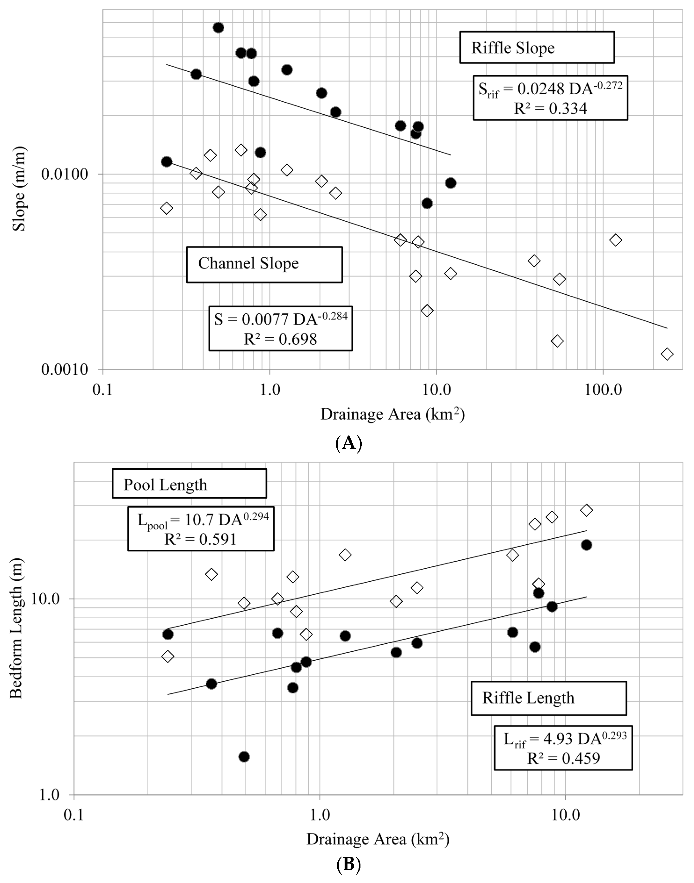
Most streams in the study area were C or E type channels based on Rosgen classification, indicated by a meandering pool-riffle morphology. Both of these classifications denote low-gradient, meandering channels with broad valleys and alluvial soils [11]. Several of the streams had width/depth ratios of 10–14 and were borderline C or E channels. This type of variability suggests these streams lie in an area of geomorphic transition, a phenomenon observed by other researchers in the Piedmont, again likely a result of historical land use and subsequent floodplain fill [25].

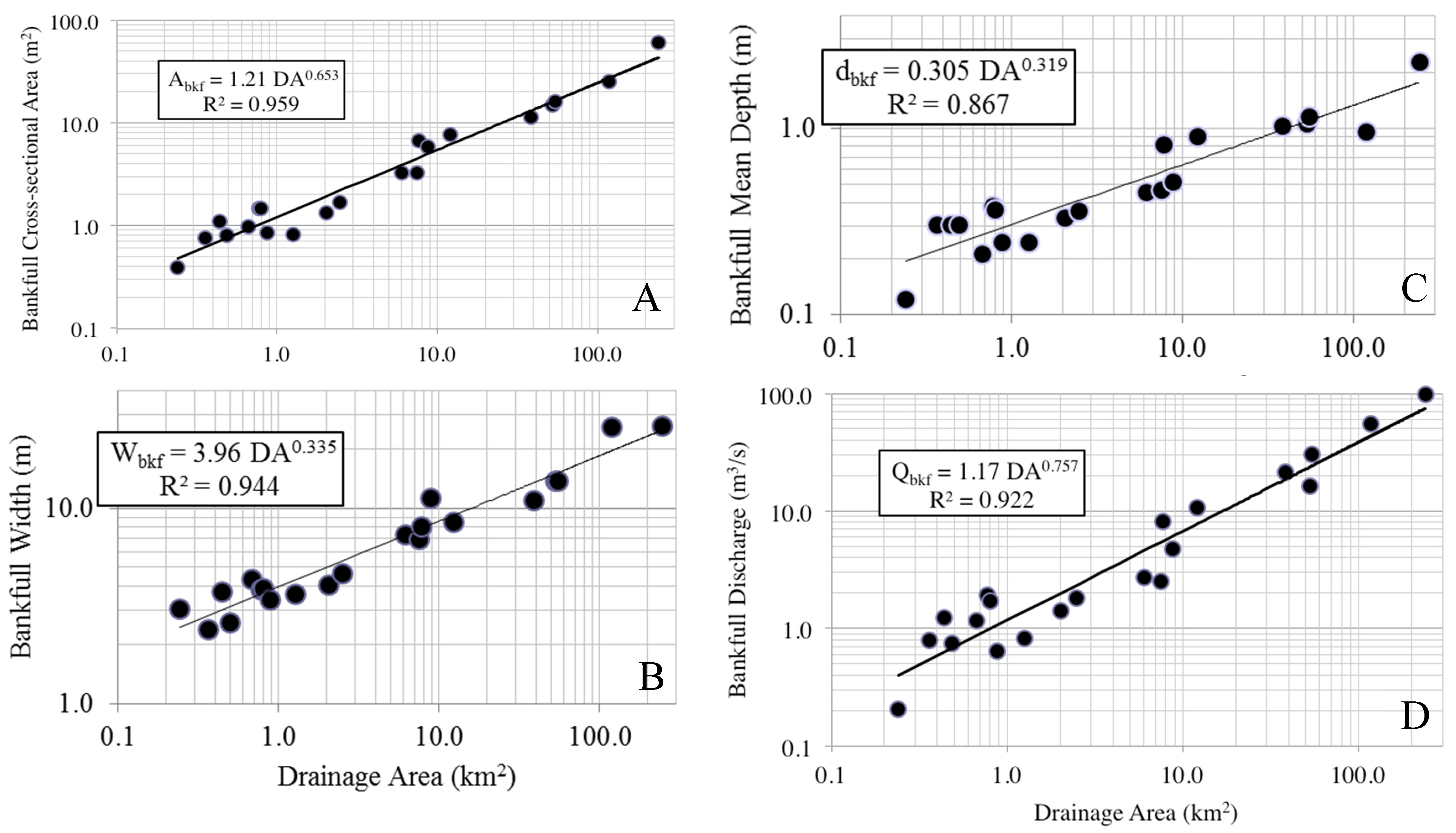
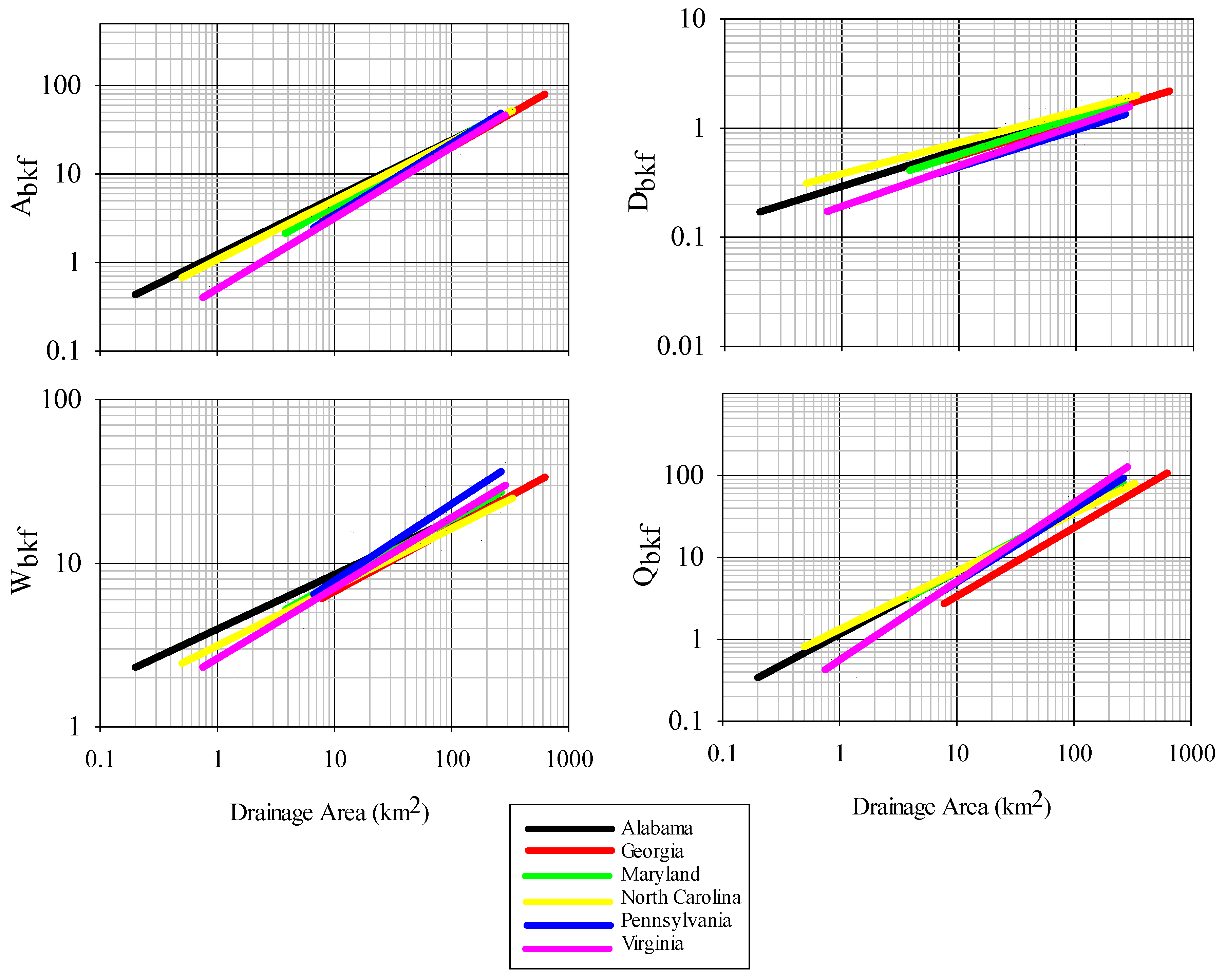
Regional bankfull curves were of high predictability, with A_bkf, W_bkf, d_bkf, and Q_bkf all largely explained by drainage area, a result similar to other studies in this region and beyond [7,29,36]. Parameter estimates for all bankfull measures were within reported values from other studies in the Piedmont region for other states, however there were some differences, particularly for curves of bankfull area, width, and discharge between this study and those generated for Virginia and Pennsylvania. Variation in bankfull relationships have been reported across the Piedmont ecoregion, with higher bankfull discharge per drainage area in the northeast as compared to the southwest Piedmont, a phenomenon potentially resulting from higher runoff in the northeast Piedmont [25]. We cannot confirm whether this also explains differences observed between Alabama and Virginia, although it is possible. Despite the causal factors, this regional variation in observed relationships is important to identify and leads to a more refined tool over broad-scale regional curves when considering restoration designs to match local reference conditions [9]. The current set of regional curves for bankfull channel dimensions thus provides a reliable tool for verifying bankfull stage in field surveys and for estimating dimensions for stream restoration projects in the Piedmont of Alabama.

Riffles and pools can provide channel stability by minimizing energy loss, and their spacing and overall channel longitudinal profile can influence many physical and biotic processes within streams [45,46] For the Alabama Piedmont, riffle and pool lengths were positively related to drainage area, however displaying considerably more variation than what was observed with bankfull cross-section dimensions. This perhaps is not surprising as fine scale geomorphic features such as riffles and pools can be heavily influenced by flow obstacles induced by local geology, gradient, plant growth and animal activity, among other sources [47,48,49]. This variation in riffle-pool morphology may be particularly true for the Piedmont ecoregion in general, given its geologic diversity, local topographic variation, and high biological diversity [20,50].

4.2. Biota

The influence of drainage area on the biotic composition of associated streams has been recognized for decades, with the river continuum concept being the most familiar framework for predictions of assemblage structure and ecosystem function considering placement within the watershed [51]. More recently the complexities and true interactive nature between geomorphic processes and ecological components have been addressed, emphasizing the role of local scale phenomena [15,49,52,53]. Our results demonstrate that biotic assemblage structure is highly correlated with drainage area and many measures of bankfull dimensions, and as such are useful benchmarks for evaluating the need and/or success of restoration efforts in the Piedmont and beyond.

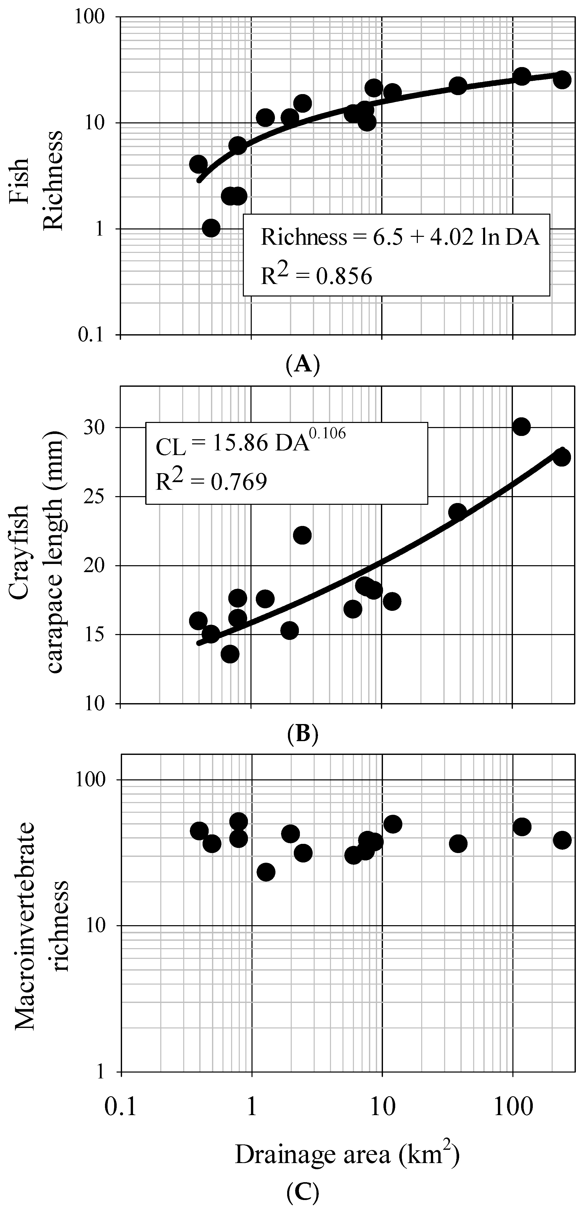
From our data, fish assemblages generally increase in richness and diversity and change rapidly in structure as stream systems initially increase in size, however these dynamics slow as system size continues to increase. There is a predictable, depauperate 2–3 species fish assemblage in small, 0.4–0.5 km² streams of this area, but assemblages increase to 10 species or more at 1 km² drainage area and to 20 species by 10 km² drainage area. Beyond 10 km² drainage area however, there is little change in species number, suggesting a potential cap in terms of fish diversity. Further, many measures of functional assemblage structure were strongly related to drainage area and measures of bankfull dimensions. Of particular note is the contribution of endemism to these patterns. The Mobile Basin has a high level of endemism in regards to fish, with the Tallapoosa claiming six species [54,55]. While these species are narrowly constrained geographically, they are often found in high abundance locally. In our sites, small- to mid-sized streams had high proportions of narrow-endemics (i.e., Tallapoosa River basin endemics). This justifies the need for conserving and restoring small streams, as they often harbor many idiosyncratic taxa and contribute disproportionately to the overall biodiversity within a basin [56]. Interestingly, broad endemics (i.e., Mobile basin endemics) were absent from the smaller streams yet were found in increasing proportions in streams with drainage areas 8 km² and higher. This provides an identifiable biological ceiling, and if these assemblages are indeed indicative of reference condition, then this ceiling can provide a powerful biotic benchmark in the assessment of success and need of restoration from a biological perspective.

Invertebrate taxa also showed a predictable response patterns across the study streams. Our results suggest that average crayfish size increases as stream systems increase in size. Also, crayfish abundance (as interpreted from CPUE) significantly decreases with increasing channel size. Indeed juvenile crayfish and smaller sub-adults are often found in shallow habitats and vegetated refugia typical of small streams, where they presumably are partly released from predation by fish. Conversely, larger crayfish are susceptible to terrestrial predators and simultaneously less susceptible to fish predation, thus can often be found in deeper waters more common in high order streams [57,58]. Interestingly, M:F ratios increased with drainage area as well, possibly reflecting increased migration and dispersal of large males, a pattern that has been observed in other systems [59]. However, sampling efficiency declines with increasing stream size due the inherent complexities of increased depth, flow, and habitat, thus to what degree observed crayfish patterns reflect a sampling bias or a true biological phenomena are unknown. Although crayfish assemblages are likely not as strong an ecological response signature as fish assemblages because of their inherently lower taxonomic diversity, these results do suggest that certain components of crayfish biology can be reasonably predicted with changing bankfull channel dimensions.

Somewhat surprisingly, our results suggest aquatic insect taxa richness and diversity do not predictably change in terms of channel dimensions over the study sites. This is surprising as macroinvertebrate taxonomic diversity and richness are typical biological response indicators of various environmental conditions [60]. As such, their use as a design and assessment tool may be limited in this area, at least compared to fish. It also should be noted that all of the streams were considered reference condition, and that the major axis of change was system size. Thus taxonomic richness/diversity may be too coarse of a measure for these purposes, although the measures do provide a biological ceiling that appears to be consistent irrespective of drainage area or geomorphology in reference condition. Trends found with compositional measures (e.g., scraper richness, % collector/filterers, etc.) however are likely more nuanced and more informative as they incorporate the functional response to physical change associated with increasing system size. Indeed collector/filterer and scraper richness significantly increased with measures of increasing system size whereas shredder richness decreased. This is in concordance with general theory regarding functional shifts in macroinvertebrate assemblages as stream systems become larger [50]. Based on observations, low-order streams in this area appear detritus-driven and tightly coupled with organic inputs from the surrounding watershed, whereas higher-order streams contain higher abundances of fine-particulate organic matter and periphyton growth. These changing environmental conditions influence assemblage structure in a predictable way and this structure can be used as a benchmark for design and assessment tools that may be used to estimate the range of aquatic insect assemblage composition in restoration projects. Although designers should consider natural variability in these data, particular attention should be paid to the lower bounds of positive relationships as they represent the critical biological ceiling across these systems.

Overall, fishes appear to have more promise than crayfishes or aquatic insects at this stage as an ecological endpoint for restoration design and assessment tools, at least in the context of this effort. However, all three groups have value in determining the ‘biological ceiling’ of reference condition in this area, and can be useful as such. The lack of strong relationships with aquatic insects may be a result of a disparity in scales, as macroinvertebrates are small-bodied organisms responding to fine-scale environmental phenomena (<10 m), and our measures of geomorphology were at the reach scale (100 m). Such disparities in scale among various taxonomic groups and environmental predictors have been implicated in other studies [61]. Scale mismatch issues may explain why we observed stronger relationships with fish than insects, as fish are considerably more mobile in water and likely respond to broader-scale phenomena, on par with geomorphology measurements.

4.3. Determination of Reference Conditions

Identifying reference condition, whether for restoration efforts, developing indices of biotic or ecological integrity, or other endeavors needing a point of reference, is a challenging yet integral issue for the effective management of ecological systems [19,62,63]. Reference conditions are used to determine restoration goals, assess the relative success of restoration efforts, and provide general context of the current ecological or physical state to that of a relatively pristine, undisturbed state. Several perspectives have been used to identify reference condition, including historic condition, best attainable condition, and least disturbed condition approach [63]. Additionally, there are multiple methods of estimating this condition, including reference site approach, best professional judgement, comparison with historical conditions, among others [63]. In this study, the streams evaluated would best be described as “least disturbed” as there are few (if any) entirely reference condition stream remaining in the southeastern Piedmont due to the current and historic land use of the area [19]. Further, identification of biological reference conditions generally proved to be highly variable as compared to reference geomorphic condition. However this is not surprising given the stochastic nature of aquatic assemblages. Of particular interest however is the strong relationships observed with taxonomic and functional measures of stream fish assemblages and drainage area. These measures have high potential to be useful as biological benchmarks, and in conjunction with predictable geomorphological benchmarks, can be effective ecological benchmarks for restoration efforts in this region.

The tools derived from this study will be useful in site assessment, project selection, restoration design and implementation, and follow-up monitoring for evaluating the success of ecosystem restoration projects in the Appalachian Plateau. They can also serve as context and point of reference for similar efforts elsewhere, perhaps ultimately leading to the development of regional ecological endpoint curves. Development of such tools that integrate ecological conditions will result in improved stream evaluations and designs increasing the effectiveness of stream restoration projects and thus improved watershed functions.

References

1. Woolsey, S.; Capelli, F.; Gonser, T.O.M.; Hoehn, E.; Hostmann, M.; Junker, B.; Paetzold, A.; Roulier, C.; Schweizer, S.; Tiegs, S.D.; et al. A strategy to assess river restoration success. Freshw. Biol. 2007, 52, 752–769. [Google Scholar] [CrossRef]
2. Doyle, M.W.; Douglas Shields, F. Compensatory mitigation for streams under the clean water act: Reassessing science and redirecting policy. J. Am. Water Resour. Assoc. 2012, 48, 494–509. [Google Scholar] [CrossRef]
3. Doll, B.A.; Jennings, G.D.; Spooner, J.; Penrose, D.L.; Usset, J.L. Evaluating the eco-geomorphological condition of restored streams using visual assessment and macroinvertebrate metrics. J. Am. Water Resour. Assoc. 2015, 51, 68–83. [Google Scholar] [CrossRef]
4. Roni, P.; Hanson, K.; Beechie, T. Global review of the physical and biological effectiveness of stream habitat rehabilitation techniques. North Am. J. Fish. Manag. 2008, 28, 856–890. [Google Scholar] [CrossRef]
5. Leopold, L.B.; Maddock, T., Jr. The Hydraulic Geometry of Stream Channels and Some Physiographic Implications; U.S. Geological Survey Professional Paper No. 252; U.S. Government Printing Office: Washington, DC, USA, 1953.
6. Dunne, T.; Leopold, L.B. Water in Environmental Planning; Macmillan: San Francisco, CA, USA, 1978. [Google Scholar]
7. Cinotto, P.J. Development of Regional Curves of Bankfull-Channel Geometry and Discharge for Streams in the Non-Urban, Piedmont Physiographic Province, Pennsylvania and Maryland; US Department of the Interior, US Geological Survey: Reston, VA, USA, 2003; p. 27.
8. Arnold, J.G.; Srinivasan, R.; Muttiah, R.S.; Williams, J.R. Large area hydrologic modeling and assessment part I: Model development. J. Am. Water Resour. Assoc. 1998, 34, 73–89. [Google Scholar] [CrossRef]
9. Bieger, K.; Rathjens, H.; Allen, P.M.; Arnold, J.G. Development and evaluation of bankfull hydraulic geometry relationships for the physiographic regions of the United States. J. Am. Water Resour. Assoc. 2015, 51, 842–858. [Google Scholar] [CrossRef]
10. Bernhardt, E.S.; Palmer, M.A. Restoring streams in an urbanizing world. Freshw. Biol. 2007, 52, 738–751. [Google Scholar] [CrossRef]
11. Rosgen, D.L.; Silvey, H.L. Applied River Morphology; Wildland Hydrology: Pagosa Springs, CO, USA, 1996; Volume 1481. [Google Scholar]
12. Lave, R. The controversy over natural channel design: substantive explanations and potential avenues for resolution. J. Am. Water Resour. Assoc. 2009, 45, 1519–1532. [Google Scholar] [CrossRef]
13. Poole, G.C. Stream hydrogeomorphology as a physical science basis for advances in stream ecology. J. North Am. Benthol. Soc. 2010, 29, 12–25. [Google Scholar] [CrossRef]
14. Sullivan, S.M.P. Geomorphic-ecological relationships highly variable between headwater and network mountain streams of Northern Idaho, United States1. J. Am. Water Resour. Assoc. 2012, 48, 1221–1232. [Google Scholar] [CrossRef]
15. Sullivan, S.M.P.; Watzin, M.C.; Hession, W.C. Understanding stream geomorphic state in relation to ecological integrity: Evidence using habitat assessments and macroinvertebrates. Environ. Manag. 2004, 34, 669–683. [Google Scholar]
16. Sullivan, S.M.P.; Watzin, M.C.; Hession, W.C. Influence of stream geomorphic condition on fish communities in Vermont, USA. Freshw. Biol. 2006, 51, 1811–1826. [Google Scholar] [CrossRef]
17. Feld, C.K.; de Bello, F.; Doledec, S. Biodiversity of traits and species both show weak responses to hydromorphological alteration in lowland river macroinvertebrates. Freshw. Biol. 2014, 59, 233–248. [Google Scholar] [CrossRef]
18. Palmer, M.A.; Bernhardt, E.S.; Allan, J.D.; Lake, P.S.; Alexander, G.; Brooks, S.; Carr, J.; Clayton, S.; Dahm, C.N.; Shah, J.F.; et al. Standards for ecologically successful river restoration. J. Appl. Ecol. 2005, 42, 208–217. [Google Scholar] [CrossRef]
19. Wear, D.N.; Greis, J.G. Southern Forest Resource Assessment; Technical Report. Gen. Tech. Rep. SRS-53; US Department of Agriculture, Forest Service, Southern Research Station: Asheville, NC, USA, 2002; p. 635.
20. Trimble, S.W. Man-Induced Soil Erosion on the Southern Piedmont; Soil and Water Conservation Soc.: Ankeny, IA, USA, 2008. [Google Scholar]
21. Nagy, R.; Lockaby, B.G.; Helms, B.; Kalin, L.; Stoeckel, D. Water resources and land use and cover in a humid region: The southeastern United States. J. Environ. Qual. 2011, 40, 867–878. [Google Scholar] [CrossRef] [PubMed]
22. Hackney, C.T.; Adams, S.M.; Martin, W.H. Biodiversity of the Southeastern United States: Aquatic Communities; John Wiley & Sons, Inc.: New York, NY, USA, 1992. [Google Scholar]
23. Noss, R.F.; LaRoe, E.T.; Scott, J.M. Endangered Ecosystems of the United States: A Preliminary Assessment of Loss and Degradation; US Department of the Interior, National Biological Service: Washington, DC, USA, 1995; Volume 28.
24. Benz, G.W.; Collins, D.E. (Eds.) Aquatic Fauna in Peril: The Southeastern Perspective; Southeast Aquatic Research Institute Special Publication 1; Lenz Design and Communications: Decatur, GA. USA, 1997; p. 553.
25. McCandless, T.L.; Everett, R.A. Maryland Stream Survey: Bankfull Discharge and Channel Characteristics in the Piedmont Hydrologic Region; CBFO-S02–01; US Fish and Wildlife Service: Annapolis, MD, USA, 2002; p. 41.
26. Lotspeich, R.R. Regional Curves of Bankfull Channel Geometry for Non-Urban Streams in the Piedmont Physiographic Province, Virginia; US Geological Survey Scientific Investigations Report 2009–5206; US Geological Survey: Reston, VA, USA, 2009; p. 51.
27. Lydeard, C.; Mayden, R.L. A diverse and endangered aquatic ecosystem of the southeast United States. Conserv. Biol. 1995, 9, 800–805. [Google Scholar] [CrossRef]
28. Barbour, M.T.; Gerritsen, J.; Snyder, B.D.; Stribling, J.B. Rapid Bioassessment Protocols for Use in Streams and Wadeable Rivers; EPA/841/B-99/002; US Environmental Protection Agency: Washington, DC, USA, 1999.
29. Zink, J.M.; Jennings, G.D.; Alexander Price, G. Morphology characteristics of Southern Appalachian wilderness streams. J. Am. Water Resour. Assoc. 2012, 48, 762–773. [Google Scholar] [CrossRef]
30. Harrelson, C.C.; Potyondy, J.P.; Rawlins, C.L. Stream Channel Reference Sites: An Illustrated Guide to Field Technique; General Technical Report RM-245; US Department of Agriculture, Forest Service: Fort Collins, CO, USA, 1994; p. 66.
31. Zimmerman, A.; Church, M.; Hassan, M.A. Identification of steps and pools from stream longitudinal profile data. Geomorphology 2008, 102, 395–406. [Google Scholar] [CrossRef]
32. Arcement, G.J., Jr.; Schneider, V.R. Guide for selecting Manning’s Roughness Coefficients for Natural Channels and Flood Plains; United States Geological Survey Water Supply Paper 2339; United States Geological Survey: Washington, DC, USA, 1989.
33. Kolberg, F.J.; Howard, A.D. Active channel geometry and discharge relations of US piedmont and midwestern streams: The variable exponent model revisited. Water Resour. Res. 1995, 31, 2353–2365. [Google Scholar] [CrossRef]
34. Pruitt, B.A. Hydrologic and Soil Conditions across Hydrogeomorphic settings. Ph.D. Dissertation, University of Georgia, Athens, GA, USA, 2001. [Google Scholar]
35. Harman, W.H.; Jennings, G.D.; Patterson, J.; Clinton, D.R.; Slate, L.O.; Jessup, A.G.; Everhart, J.R.; Smith, R.E. Bankfull hydraulic geometry relationships for North Carolina streams. In Proceedings of AWRA Wildland Hydrology Symposium, Bozeman, MT, USA, 30 June–2 July 1999; pp. 401–408.
36. Brockman, R.R.; Agouridis, C.T.; Workman, S.R.; Ormsbee, L.E.; Fogle, A.W. Bankfull regional curves for the Inner and Outer Bluegrass regions of Kentucky. J. Am. Water Resour. Assoc. 2012, 48, 391–406. [Google Scholar] [CrossRef]
37. Frimpong, E.A.; Angermeier, P.L. Fish traits: A database of ecological and life-history traits of freshwater fishes of the United States. Fisheries 2009, 34, 487–495. [Google Scholar] [CrossRef]
38. Caton, L.W. Improved subsampling methods for the EPA “Rapid Bioassessment” benthic protocols. North Am. Benthol. Soc. Bull. 1991, 8, 317–319. [Google Scholar]
39. Vinson, M.R.; Hawkins, C.P. Effects of sampling area and subsampling procedure on comparisons of taxa richness among streams. J. North Am. Benthol. Soc. 1996, 15, 392–399. [Google Scholar] [CrossRef]
40. Merritt, R.W.; Cummins, K.W.; Berg, M.B. An Introduction to the Aquatic Insects of North America, 4th ed.; Kendall/Hunt Publishing: Dubuque, IA, USA, 2008. [Google Scholar]
41. Homer, C.G.; Dewitz, J.A.; Yang, L.; Jin, S.; Danielson, P.; Xian, G.; Coulston, J.; Herold, N.D.; Wickham, J.D.; Megown, K. Completion of the 2011 National Land Cover Database for the conterminous United States-representing a decade of land cover change information. Photogramm. Eng. Remote Sens. 2015, 81, 345–354. [Google Scholar]
42. Harding, J.S.; Benfield, E.F.; Bolstad, P.V.; Helfman, G.S.; Jones, E.B.D. Stream biodiversity: The ghost of land use past. Proc. Natl acad. Sci. 1998, 95, 14843–14847. [Google Scholar] [CrossRef] [PubMed]
43. Jackson, C.R.; Martin, J.K.; Leigh, D.S.; West, L.T. A southeastern piedmont watershed sediment budget: Evidence for a multi-millennial agricultural legacy. J. Soil Water Conserv. 2005, 60, 298–310. [Google Scholar]
44. Utz, R.M.; Hilderbrand, R.H.; Boward, D.M. Identifying regional differences in threshold responses of aquatic invertebrates to land cover gradients. Ecol. Indic. 2009, 9, 556–567. [Google Scholar] [CrossRef]
45. Gore, J.A. Benthic invertebrate colonization: source distance effects on community composition. Hydrobiologia 1982, 94, 183–193. [Google Scholar] [CrossRef]
46. Anderson, J.K.; Wondzell, S.M.; Gooseff, M.N.; Haggerty, R. Patterns in stream longitudinal profiles and implications for hyporheic exchange flow at the HJ Andrews Experimental Forest, Oregon, USA. Hydrol. Process. 2005, 19, 2931–2949. [Google Scholar] [CrossRef]
47. Clifford, N.J. Formation of riffle—pool sequences: Field evidence for an autogenetic process. Sediment. Geol. 1993, 85, 39–51. [Google Scholar] [CrossRef]
48. Wohl, E.E. Bedrock channel incision along Piccaninny Creek, Australia. J. Geol. 1993, 101, 749–761. [Google Scholar] [CrossRef]
49. Stallins, J.A. Geomorphology and ecology: Unifying themes for complex systems in biogeomorphology. Geomorphology 2006, 77, 207–216. [Google Scholar] [CrossRef]
50. Woodruff, J.F.; Parizek, E.J. Influence of underlying rock structures on stream courses and valley profiles in the Georgia Piedmont. Ann. Assoc. Am. Geogr. 1956, 46, 129–139. [Google Scholar] [CrossRef]
51. Vannote, R.L.; Minshall, G.W.; Cummins, K.W.; Sedell, J.R.; Cushing, C.E. The river continuum concept. Can. J. Fish. Aquat. Sci. 1980, 37, 130–137. [Google Scholar] [CrossRef]
52. Statzner, B.; Fievet, E.; Champagne, J.Y.; Morel, R.; Herouin, E. Crayfish as geomorphic agents and ecosystem engineers: Biological behavior affects sand and gravel erosion in experimental streams. Limnol. Oceanogr. 2000, 45, 1030–1040. [Google Scholar] [CrossRef]
53. Post, D.M.; Doyle, M.W.; Sabo, J.L.; Finlay, J.C. The problem of boundaries in defining ecosystems: A potential landmine for uniting geomorphology and ecology. Geomorphology 2007, 89, 111–126. [Google Scholar] [CrossRef]
54. Boschung, H.T.; Mayden, R.L. Fishes of Alabama; Smithsonian Books: Washington, DC, USA, 2004. [Google Scholar]
55. Neely, D.A.; Williams, J.D.; Mayden, R.L. Two new sculpins of the genus Cottus (Teleostei: Cottidae) from rivers of eastern North America. Copeia 2007, 2007, 641–655. [Google Scholar] [CrossRef]
56. Finn, D.S.; Bonada, N.; Múrria, C.; Hughes, J.M. Small but mighty: Headwaters are vital to stream network biodiversity at two levels of organization. J. North Am. Benthol. Soc. 2011, 30, 963–980. [Google Scholar] [CrossRef]
57. Rabeni, C.F. Resource partitioning by stream dwelling crayfish: The influence of body size. Am. Midl. Nat. 1985, 113, 20–29. [Google Scholar] [CrossRef]
58. Englund, G. Effects of fish on the local abundance of crayfish in stream pools. Oikos 1999, 87, 48–56. [Google Scholar] [CrossRef]
59. Wutz, S.; Geist, J. Sex- and size-specific migration patterns and habitat preferences of invasive signal crayfish (Pacifastacus leniusculus Dana). Limnologica 2013, 43, 59–66. [Google Scholar] [CrossRef]
60. Allan, J.D. Landscapes and riverscapes: The influence of land use on stream ecosystems. Annu. Rev. Ecol. Evol. Syst. 2004, 35, 257–284. [Google Scholar] [CrossRef]
61. Simpson, A.; Turner, I.; Brantley, E.; Helms, B. Bank erosion hazard index as an indicator of near-bank aquatic habitat and community structure in a southeastern Piedmont stream. Ecol. Indic. 2014, 43, 19–28. [Google Scholar] [CrossRef]
62. White, P.S.; Walker, J.L. Approximating nature’s variation: selecting and using reference information in restoration ecology. Restor. Ecol. 1997, 5, 338–349. [Google Scholar] [CrossRef]
63. Stoddard, J.L.; Larsen, D.P.; Hawkins, C.P.; Johnson, R.K.; Norris, R.H. Setting expectations for the ecological condition of streams: the concept of reference condition. Ecol. Appl. 2006, 16, 1267–1276. [Google Scholar] [CrossRef]
Figure 1. Ecoregions of Alabama (lines) and the Tallapoosa River basin (shaded). The Piedmont ecoregion is within bold lines. All 21 study sites were in the Piedmont ecoregion of the Tallapoosa basin. Upper photo typifies conditions at a small stream (0.4 km2 drainage area) and the lower photo typifies conditions at a larger stream site (118 km2 drainage area).
Water 08 00161 g001
Figure 2. Regional geomorphic curves for Alabama Piedmont reference streams. All channel dimension variables are related to drainage area by the power model y = axb, where y is channel dimension measure and x is drainage area, a is slope and b is model parameter. (A) bankfull cross-sectional area; (B) bankfull cross-sectional width; (C) bankfull cross-sectional depth; (D) bankfull discharge.
Water 08 00161 g002
Figure 3. Slope (A) and bedform (B) relationships with drainage area for Alabama Piedmont reference streams. All slope and bedform variables are related to drainage area by the power model y = axb, where y is the bedform measure and x is drainage area, a is slope and b is model parameter.
Water 08 00161 g003
Figure 4. Comparison of regional geomorphic curves across the Piedmont ecoregion of the southeast. Geomorphic variables are as in Figure 1. Source data for comparisons include Georgia [34], North Carolina [35], Virginia [26], Maryland [25], and Pennsylvania [7].
Water 08 00161 g004
Figure 5. Regional ecological endpoint curves for Alabama Piedmont reference streams. All biotic variables are related to drainage area by either a logarithmic model (fish, y = yo + a ln x) or a power model (crayfish, y = axb) where y is the biotic richness and x is the bankfull dimension measure, a is slope and b is model parameter. (A) Fish richness; (B) crayfish richness; (C) bug richness.
Water 08 00161 g005