
Understanding Persistence to Avoid Underestimation of Collective Flood Risk

1
School of Civil Engineering and Geosciences, Newcastle University, Newcastle Upon Tyne NE1 7RU, UK
2
Willis Research Network, 51 Lime Street, London EC3M 7DQ, UK
*
Author to whom correspondence should be addressed.
Water 2016, 8(4), 152; https://doi.org/10.3390/w8040152
Submission received: 12 January 2016
/
Revised: 19 March 2016
/
Accepted: 31 March 2016
/
Published: 15 April 2016
Abstract
:The assessment of collective risk for flood risk management requires a better understanding of the space-time characteristics of flood magnitude and occurrence. In particular, classic formulation of collective risk implies hypotheses concerning the independence of intensity and number of events over fixed time windows that are unlikely to be tenable in real-world hydroclimatic processes exhibiting persistence. In this study, we investigate the links between the serial correlation properties of 473 daily stream flow time series across the major river basins in Europe, and the characteristics of over-threshold events which are used as proxies for the estimation of collective risk. The aim is to understand if some key features of the daily stream flow data can be used to infer properties of extreme events making a more efficient and effective use of the available data. Using benchmark theoretical processes such as Hurst-Kolmogorov (HK), generalized HK (gHK), autoregressive fractionally integrated moving average (ARFIMA) models, and Fourier surrogate data preserving second order linear moments, our findings confirm and expand some results previously reported in the literature, namely: (1) the interplay between short range dependence (SRD) and long range dependence (LRD) can explain the majority of the serial dependence structure of deseasonalized data, but losing information on nonlinear dynamics; (2) the standardized return intervals between over-threshold values exhibit a sub-exponential Weibull-like distribution, implying a higher frequency of return intervals longer than expected under independence, and expected return intervals depending on the previous return intervals; this results in a tendency to observe short (long) inter-arrival times after short (long) inter-arrival times; (3) as the average intensity and the number of events over one-year time windows are not independent, years with larger events are also the more active in terms of number of events; and (4) persistence influences the distribution of the collective risk producing a spike of probability at zero, which describes the probability of years with no events, and a heavier upper tail, suggesting a probability of more extreme annual losses higher than expected under independence. These results provide new insights into the clustering of stream flow extremes, paving the way for more reliable simulation procedures of flood event sets to be used in flood risk management strategies.
1. Introduction
Extreme river floods are one of the major natural hazards that have affected European countries for centuries [1,2,3], causing many deaths and billions US$ damages in the last decades [4,5]. Historical records worldwide show that floods tend to cluster in time (e.g., [3,6]). This phenomenon concerning the temporal fluctuation of floods can be related to the dynamics of processes exhibiting long range dependence (LRD) or temporal persistence. This type of dynamics has widely been studied since its recognition by Hurst [7], resulting in a range of diagnostics (e.g., [8,9,10,11,12]) and modeling tools [13,14,15,16,17].
Dealing with stream flow processes, the interaction between short range dependence (SRD) and LRD can affect the recognition of the actual dynamics and the estimation of parameters summarizing SRD and LRD behavior. From a diagnostic perspective, the interplay of SRD and LRD has usually been studied attempting to separate the (small) temporal scales in which SRD acts and (large) temporal scales in which LRD dominates (e.g., [18,19]), or modifying LRD detection methods accounting for SRD (e.g., [20]). Detection and identification of SRD and LRD are also affected by the sample size. In fact, LRD is an asymptotic property of the process that should be studied on the largest scales (i.e., in the tails), and several thousand observations are required for instance to correctly estimate the Hurst parameter H (which quantifies the linear part of LRD) for signals simulated by autoregressive moving average (ARMA) models, whose behavior is SRD but mimics LRD [21,22]. In order to model stream flow fluctuations, fractional integrated autoregressive moving average (ARFIMA) models [15,16] are a classical and well-established option (e.g., [22,23,24,25,26]).
However, both analyses and models commonly focus on the overall process (e.g., daily or monthly stream flow), while extreme values are investigated as a by-product. In the last decade, more attention has been paid to the statistics (magnitude and frequency of occurrence) of extreme values of persistent processes (e.g., [27,28,29] and references therein ). Such works investigated (monofractal) processes characterized by autocorrelation functions with power-law decay or (multifractal) processes exhibiting nonlinear temporal dependence structure and vanishing linear autocorrelation (e.g., [30,31]). Based on that theoretical framework, Bogachev and Bunde [32] analyzed 32 long stream flow time series recorded worldwide, and found that the empirical distributions of the standardized return intervals (or inter-arrival times) between extremes exceeding high (percentile) thresholds collapse into a set of patterns depending only on the threshold, but not on the location, and well described by gamma-type distributions. They also showed that such empirical distributions are well reproduced by the corresponding empirical distributions of data of the same length drawn from a process with power-law decaying autocorrelation function with a unique effective exponent , whereby the exponent differs from the measured correlation exponent ξ (which ranges between 0.4 and 0.8) owing to the interplay between linear and nonlinear dependence in the data and the finite-size effects [32]. For the stream flow records analyzed, the authors also highlighted that H ranges between 0.6 and 1.
Therefore, since the distribution of the return intervals can be parameterized by the autocorrelation exponent ξ, and ξ is related to H for a number of theoretical processes (some of which are used in the following sections), the estimation of H is a key aspect to define a link between the overall process (e.g., daily stream flow) and the behavior of the corresponding extreme values. As mentioned above, several methods are available to infer LRD and compute H, and studies conducted on worldwide long stream flow records using different approaches highlighted that stream flows are generally characterized by at large time scales [18,19,22,32,33,34,35,36].
Since the persistence properties of complex river systems impacts on natural hydrological variability in a changing environment [3,6], this study further investigates the link between SRD/LRD, simple but informative models reproducing such properties, and the occurrence statistics of the corresponding extreme values. Based on the increasing importance of insurance and reinsurance as non-structural methods to hedge against natural hazards, we treat the topic considering some key properties that should be taken into account to develop modeling strategies improving current risk assessment procedures. In this respect, the assessment of the so-called collective risk is a typical problem faced in insurance and reinsurance practice. Dealing with floods, for a fixed flood-prone area, the collective risk is the total claim amount regarding the portfolio of (re)insured properties as a collective that produces a random number N of claims in a certain time period (e.g., one year) [37] (p. 41).
In this study we investigate the dynamics of daily stream flow series from a collective risk viewpoint, treating the exceedances over given thresholds as proxies for claim amounts, and defining as the accumulation of claim amounts over fixed one-year time windows. In more detail, we study the properties of the return intervals R between over-threshold events, the number N of exeedances, and . These characteristics are therefore interpreted in terms of temporal persistence to link the behavior of the extreme values to that of the whole process, in order to pave the way for modeling approaches of extreme values based on a more efficient use of the information contained in the entire sequences of data. The paper is organized as follows: data sets and methods are presented in Section 2, empirical results are shown in Section 3, and concluding remarks are summarized in Section 4.
2. Data and Methodology
2.1. Data
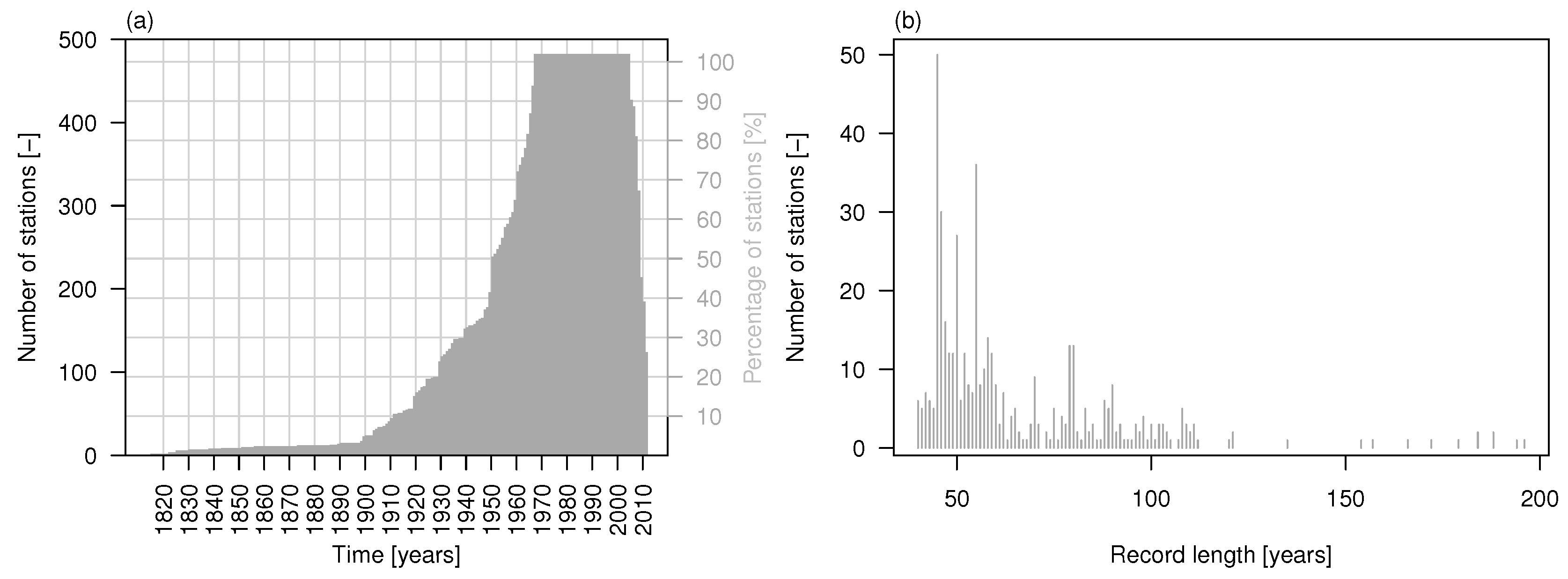
The data set comprises 473 daily stream flow time series across the major basins in Europe (data obtained from the Global Runoff Data Centre (GRDC), Federal Institute of Hydrology, Koblenz, Germany). The time series were selected in order to have the maximum number of sequences with maximum temporal overlap (namely, 37 years from 1968 to 2005) and less than 10% of missing values. Figure 1 shows the study area and stream gage locations, while the time series of the number of stations available in a given year (out of 473) and histogram of the record length for the 473 stations are shown in Figure 2. The list of stations and related information are provided in the supplementary material (Table S1).
2.2. Methods
As the stream flow series exhibit positively skewed marginal distributions and strong seasonality that depends on climatic zones and basin response dynamics, the data are preliminary transformed and deseasonalized by the following procedure. Data are transformed to normality by normal quantile transformation (NQT) , where denotes the inverse of the standard Gaussian cumulative distribution function, is the Weibull version of the empirical cumulative distribution function, is the indicator function, and T is the sample size.
For a given sequence of stream flow observations , , the empirical average value for each calendar day and the calendar-day standard deviation are computed. The seasonal components and are then smoothed by local scatter plot smoothing (LOESS) [38] following the rationale of the seasonal-trend decomposition based on LOESS (STL) procedure [39], obtaining smoothed seasonal components and . Thus, deseasonalized time series are obtained by subtracting from and then dividing by as follows
As is well known, this procedure removes the seasonality of the first two moments of the time series and is standard in hydrological analyses (e.g., [16,19,23,25] among others). The marginal transformation is performed to rectify heteroskedasticity and non-normality of the residuals of the models fitted to the deseasonalized time series [16] (pp. 464–465). The deseasonalization is applied to mitigate the effect of seasonality on subsequent analyses.
To characterize the dynamics of extreme stream flow values, we performed an over-threshold selection using three different percentage thresholds (95%, 98%, and 99%), making the analysis independent of the specific site and allowing a sensitivity study of the results. We therefore defined the inter-arrival times or return intervals r between subsequent observations exceeding the threshold(s) . It should be noted that the sequences of values day indicate periods with stream flow exceeding , while the return intervals denote the durations of periods with . Our analyses focus on the latter subset of r values which properly define the inter-arrival time between blocks of extreme values. To allow a better comparison and recognition of a possible general behavior (e.g., [29,30,31,32,40,41]), for each time series and each threshold, the sequence of r values is standardized dividing by the return period (i.e., the mean return interval) , where is the number return intervals . It is known that the statistics of return intervals r of extreme values are related to the nature of the underlying process. For example, for processes with LRD and autocorrelation function decaying as a power law of lag τ, is characterized by a stretched exponential (Weibull) distribution and finite-size effects for and power-law distribution and discretization effects for (e.g., [28,29] and references therein).
where denotes the probability density function of r for a given threshold , , and is a scale parameter depending on ξ (e.g., [29]). Notice that a power-law distribution for characterizes multifractal signals (e.g., [31]).
These links between the behavior of extreme events and the underlying process allow in principle a more efficient use of the available information (e.g., daily stream flow) to infer and set up modeling and simulation strategies for the extremes. The statistics of the values for the stream flow data are therefore compared with those corresponding to a set of models in order to interpret the properties of the records and identify parsimonious candidate models able to reproduce the main properties of the observed return intervals of stream flow extremes. To simulate time series allowing for a fair comparison taking into account both discretization and finite-size effects, we used a set of parametric and nonparametric models/methods: (1) ARFIMA(), where p, d, and q denote the autoregressive order, the fractional order of differencing, and the moving average order, respectively (e.g., [14,23,25,42]); (2) fractional Gaussian noise (fGn; [13,43,44,45,46]), also known as Hurst-Kolmogorov process (HK; [47,48]), which is parameterized by the so-called Hurst exponent H; (3) a generalization of the HK process (gHK; [17]), which involves an additional parameter λ and allows for mixing Markov SRD behavior and HK LRD dynamics; and (4) iterative amplitude adjusted Fourier transformation (IAAFT; [49,50,51,52,53]).
ARFIMA models are a classical option allowing the reproduction of both SRD and LRD and a variety of temporal dependence structures. However, these models rely on the introduction of additional terms to the simplest versions and show some drawbacks, such as definition in discrete time that may not necessarily correspond to a continuous-time process, over-parametrization contradicting the principle of parsimony, identification usually based on the autocorrelation function (ACF), which is known to be highly biased [54].
The special case ARFIMA() describes processes with hyperbolically-decaying autocorrelation function close (but not identical) to the HK process. These models are quite flexible in reproducing temporal persistence, and their parameters are related by . The slope ξ of the autocorrelation function of ARFIMA() and HK is proportional to d and H, respectively. However, the HK process shows some properties which are not physically realistic, such as the infinite variance of the instantaneous process [54]. In order to overcome these drawbacks, some extensions have been proposed, e.g. the HK process with low scale smoothing [55], a hybrid HK process [54], and gHK. In particular, the continuous gHK is a three-parameter process defined by the autocovariance function [17]:
where λ has dimension and denotes the variance of the process, q has dimension and indicates the limit between HK processes and those affected by the minimum scale limit of the process , and is dimensionless and controls the LRD behavior. The function in Equation (3) decays exponentially for small time lags and algebraically (i.e., as a power law) for large scales; thus, it mimics Markovian behavior in the short term and HK persistence in the long term. Such a process provides a suitable, parsimonious and physically consistent option to high-parameterized ARFIMA models for daily stream flow dynamics.
IAAFT allows the simulation of surrogate data preserving almost exactly the empirical distribution function and power spectrum of the observations. IAAFT is often used in nonlinear dynamics studies to simulate surrogate data to be used to test nonlinear behavior. IAAFT surrogates are stationary [56] and temporally symmetric by construction because of randomization of Fourier phases, meaning that the sampling algorithm does not preserve the forward-backward asymmetry related to the different dynamics of the hydrographs’ rising limb and recession branch (which are driven by meteorological forcings and basin response, respectively). Thus, since IAAFT is data driven and the estimated power spectrum is the reference “truth” and contains no information about the direction of time, IAAFT allows us to explore the properties of r and for resampled time series which preserve the moments up to the second order excluding time irreversibility, which is strong signature of nonlinearity. A simple measure of asymmetry of a time series under time reversal is the third order quantity [51]
where denotes the deseasonalized records, T is the sample size, and τ is the lag. The summary statistic in Equation (4) can be seen as an index of temporal skewness and therefore be used to check time irreversibility in both observed and simulated series. Of course, alternative but similar measures of asymmetry such as the volatility can be used [57].
Among the diagnostic methods that are available to explore the temporal dependence structure of daily stream flow series (e.g., [8,9,11,12]), we considered the aggregated variance analysis (also known as climacogram; [17,47,58]) and the detrended fluctuation analysis (DFA; [59]). Climacogram describes the variance of the time averaged process as a function of time scale, and allows the analytical computation of the estimation bias to be included in the model identification and fitting [54]. Climacogram can be used to fit the gHK parameters following for instance the two-stage procedure suggested by Dimitriadis and Koutsoyiannis [17] and summarized in the Appendix. DFA belongs to the class of scaled windowed variance (SWV) methods which are similar to the climacogram, but measure the variance of integrated fGn-like signals by dividing the series into subsamples (or time windows or blocks) of size k resulting from a forward and backward partition of the time series [10,60], and computing the mean of the subsample variances instead of the variance of the subsample means. is the variance of the fluctuations (residuals) from local trends fitted in each subsample. These local trends are defined as local linear or polynomial regressions in DFA (a three-order polynomial is used in this study) [10,59,60,61]. It should be noted that LRD diagnostics are commonly affected by the presence of seasonal/cyclic patterns [6,62,63,64,65,66]; therefore, the deseasonalization procedure in Equation (1) provides a simple but effective way to handle this aspect.
To assess the impact of SRD, LRD and nonlinearity on the temporal collective risk, are treated as proxies of insurance claims, and is defined as
where is the jth claim proxy (over-threshold flow fluctuation severity), and the total claims if . A classical assumption on the aggregate amount is to require that N and the individual claims are independent and identically distributed, and also that N and all claim amounts are independent to each other; therefore, this study investigates the effects of lack of fulfillment of these assumptions on .
3. Results
In this section, we first discuss some general remarks concerning the observed and simulated time series using simple time series plots and referring to a single sequence of records, and then we present results concerning the entire data set in more detail.
3.1. Preliminary Remarks
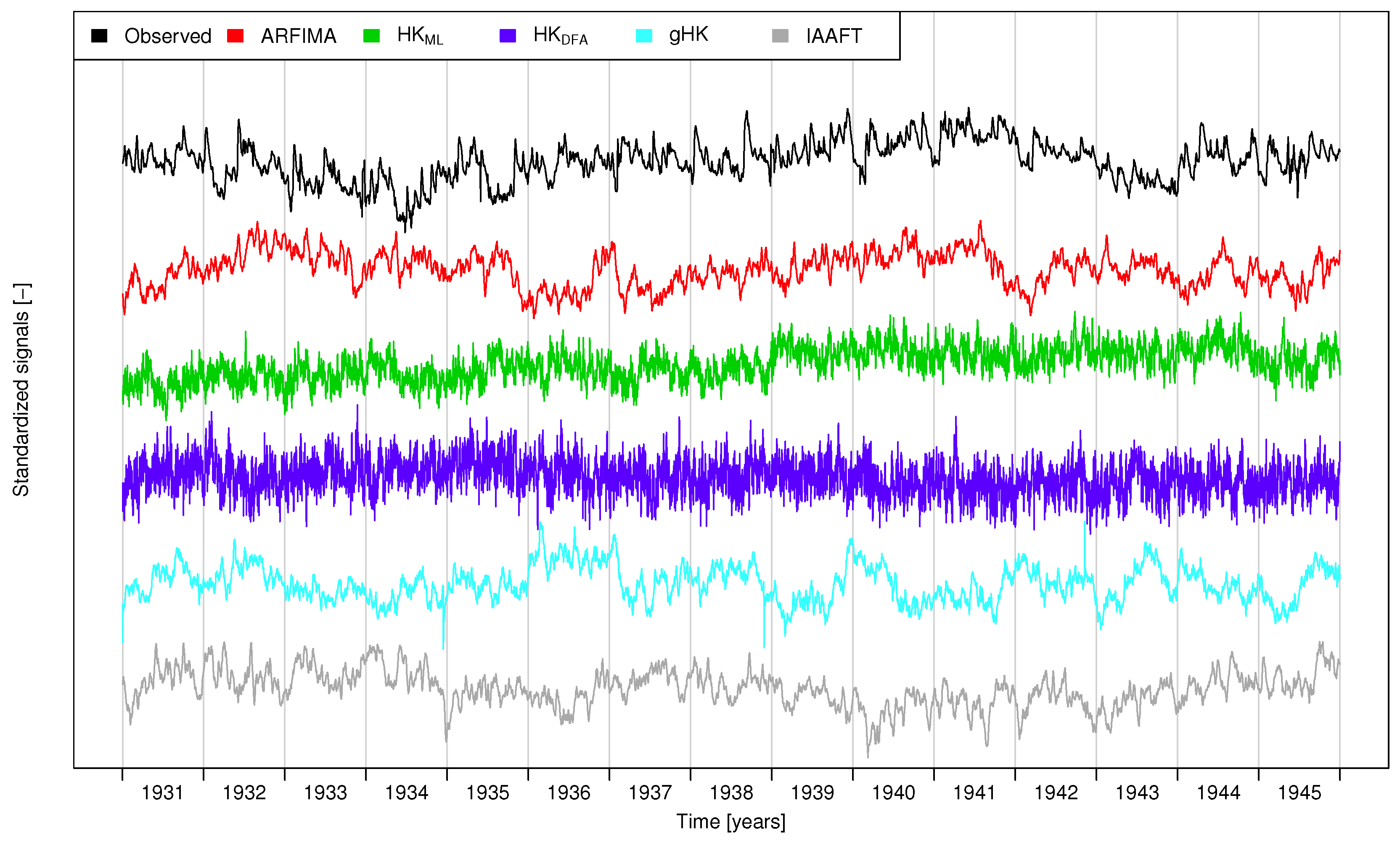
For the sake of illustration, Figure 3 shows the time series of the first 15 years of daily flows and surrogate signals corresponding to the Elbe River at Magdeburg-Strombruecke (GRDC ID 6340180).
Figure 3 highlights that the stream flow fluctuations are characterized by local (intra-annual) and global (inter-annual) trends resulting in sequences of flood-rich and flood-poor years [3], which is a typical behavior for processes showing LRD, as is confirmed by the patterns of the series simulated by ARFIMA,HK, gHK and IAAFT. In more detail, since in the present context we are not looking for the optimal model structure, in this study we have used an ARFIMA model, which is flexible enough to describe the dependence structure of the 473 signals even though it is not parsimonious. For HK, we have used two different estimators of H: the maximum likelihood (ML) estimator [67,68], and the values obtained by DFA focusing on time scales greater than ≈300 days to account for the effect of SRD [19] on the estimation of H. Even though HK signals in Figure 3 capture some key features of the observed sequences, such as inter-annual fluctuations, they are not able to account for SRD, thus resulting in a lack of local smoothness, which instead characterizes . This shortcoming is overcome by introducing the SRD component. In particular, IAAFT and gHK sequences resemble the observations very closely, whereas the ARFIMA signal preserves some lack of smoothness at short terms likely due to the MA components. However, while the agreement with IAAFT is expected as the resampling algorithm guarantees the almost perfect preservation of the empirical power spectrum and marginal distribution, the performance of the gHK model is remarkable if we consider that the model has only three parameters.
As mentioned in Section 2.2, all the approaches used to mimic the sequences are not able to preserve temporal asymmetry. To make a quantitative check, we have computed the temporal skewness in Equation (4) for the Elbe time series and different lags τ. The significance of the values was checked by computing the 95% confidence intervals (CIs) under two different conditions, namely, temporal independence and preservation of the second order properties. Under the first assumption, CIs have been computed by shuffling (randomizing) the original time series (thus, destroying the temporal dependence structure but preserving the marginal distribution) times, then calculating for different lags, and finally computing the empirical 2.5th and 97.5th percentiles over the B values of for each lag. Under the second condition, the randomization is replaced by IAAFT resampling. Figure 4 shows that the series exhibits significant temporal irreversibility denoted by values characterized by a persistent sign (positive or negative), and exceeding the CIs at several lags. This conclusion holds for both conditions (lack of serial correlation, and preservation of second order properties) and is considered a signature of the nonlinearity of stream flow dynamics. Of course, IAAFT CIs are wider than shuffled CIs owing to the variance inflation effect of the serial correlation, which however is not sufficient to explain the observed values. Similar results hold true for the other time series (not shown).
3.2. Climacogram Analysis and DFA: Highlighting SRD and LRD
Figure 5 shows the empirical climacogram (circles) corresponding to the Elbe River signal in Figure 3, and the theoretical climacograms corresponding to AR(1), HK and gHK with parameters fitted on the data. The diagram highlights that neither SRD nor LRD models provide a satisfactory fitting, while their combination describes the empirical behavior very well. To further check the suitability of gHK and the other methods, we simulated one time series for each model/method (fitted on the data) and compared the empirical climacograms of the synthetic series with the theoretical climacograms fitted on the original sequence (Figure 5a). Figure 5b–f shows that ARFIMA, gHK and IAAFT yield time series whose climacogram is very close to the theoretical gHK and the original empirical one. This result is expected for IAAFT, which preserves the second order properties by construction, and confirms that gHK is a parsimonious and effective physically consistent alternative to high-parameterized ARFIMA models. Of course the empirical climacogram of the HK signal is close to its theoretical counterpart for the ML estimate of H (Figure 5c), whereas a HK process with H estimated by DFA exhibits remarkable discrepancies (Figure 5d).
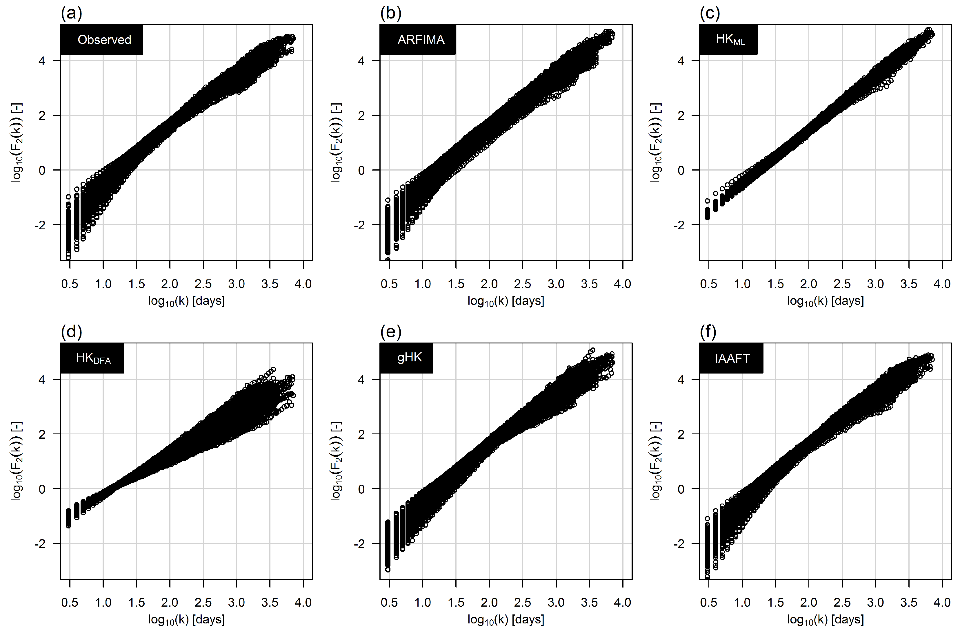
It should be noted that the DFA-based H value was estimated over time scales larger than days to account for the crossover of the scaling properties occurring at time scales below ≈1 year (e.g., [18,19] and references therein). To better understand this point and its effect on modeling, Figure 6 shows the diagrams of the average values of the variance fluctuations versus the corresponding aggregation time scales k. If the signal has a simple scaling behavior is expected to scale as , where is the so-called generalized Hurst exponent for the moment of order m, and yields the Hurst parameter for and stationary processes (e.g., [10]). Each panel of Figure 6 shows the patterns of the ensemble of functions corresponding to the 473 time series (observed or simulated). The crossover in the “observed” is well reproduced by gHK and IAAFT. ARFIMA yields some discrepancy, whereas HK does not exhibit crossover (as expected). To quantify the crossover, was computed for each function and two sets of time scales: and .
Figure 7 highlights that the values follow two different statistical distributions for the two classes of time scales, and ARFIMA, gHK and IAAFT are able to reproduce this behavior, whereas HK models (with ML and DFA estimates of H) do no reproduce the crossover at all (since , we refer to Serinaldi [11] and references therein for the interpretation of DFA H values greater than unity). These results are in agreement with those reported by Kantelhardt et al. [19] with differences mainly related to a different choice of the crossover time scale, and confirm that the crossover results from the interplay of SRD and LRD, rather than residual seasonality as is sometimes argued in the literature [65]. Compared with previous studies, the crossover attribution relies on the use of models that explicitly account for both SRD and LRD with different degrees of complexity, and allow the simultaneous reproduction of short and long term dynamics, thus further strengthening conclusions concerning the nature of the crossover.
The use of ARFIMA and gHK allows also the study of the effect of the simultaneous estimation of the additional parameters involved in ARFIMA and gHK models on H estimates compared with H values resulting from DFA (where H is the only target parameter). The main diagonal of panels in Figure 8 shows the distributions of H obtained by DFA (), gHK (), and ARFIMA (). The distribution of values is coherent with DFA results reported in the literature for different stream flow data sets (e.g., [19,35]). On the other hand, the additional parameters of ARFIMA and gHK strongly change the H distribution resulting in and of and values, respectively, in the range , thus indicating that the simultaneous estimation of SRD and LRD components tend to favor SRD in several cases; however, this is not surprising when dealing with finite samples.
The pairwise scatter plots and the values of the Kendall correlation coefficient in the upper triangular matrix of panels in Figure 8 show that only and are correlated. The spatial distribution of the H values (lower triangular matrix of panels in Figure 8) shows that exhibit a coherent pattern with lower values around the Alpine area and upper Danube, and larger values in the northern part of the study area and lower Danube. Therefore, persistence tends to coherently emerge in lower part of the large rivers flowing in the plain areas of northern Europe and lower Danube, and is less evident in the smaller rivers flowing in the mountainous/hilly areas of southern France, Alps, and upper Danube. The spatial pattern is less evident or lost for and as LRD components in these models are influenced by the SRD part.
The parameterization of gHK allows further remarks. The upper triangular matrix of panels in Figure 9 shows that is positively correlated with λ (which summarizes the variance of the discrete process at the smaller aggregation scale) and negatively correlated with q (which describes the scale where LRD behavior emerges). Therefore, signals showing higher persistence tend to show higher variance at the finest time scale k (for the discrete process). Moreover, the higher the persistence and the variance (at the finest time scale) the earlier LRD tends to emerge (i.e., the smaller q is) superseding SRD dynamics. The parameters show no particular spatial patterns (lower triangular matrix of panels in Figure 8).
3.3. The Effect of Persistence on Return Intervals’ Statistics
Based on the results above we retained only ARFIMA, gHK and IAAFT for further analysis concerning return intervals. Denoting the cumulative distribution function of r, the properties of r are summarized by the diagrams of the negative logarithm of the survival function versus in log-log plot, as the exponential and Weibull distributions reduce to straight lines, making the assessment of fitting easier. Figure 10 shows the ensemble of survival functions of the rescaled return intervals corresponding to the 473 time series included in this study for the percentile threshold (black circles). Similar results hold for the other thresholds, but with higher uncertainty owing to the smaller number of over-threshold events (see Figures S1 and S2 in the supplementary material). Each plot in Figure 10 also shows the standard exponential distribution (blue line), the Weibull distribution with shape parameter corresponding to the average value of H computed by the LSV method for the gHK model (red line), and the ensemble of survival functions corresponding to time series simulated by different models (grey circles).
In more detail, Figure 10a reports the empirical survival functions corresponding to samples simulated by a Weibull distribution for r with shape parameter related to the H value of the underlying time series. Figure 10b refers to shuffled time series and highlights the suitability of the exponential model under the hypothesis of temporal independence. Figure 10c–e refers to the distributions of the return intervals of extreme events extracted from time series simulated by ARFIMA, gHK, and IAAFT. For , return intervals tend to follow a Weibull distribution and data points collapse, thus denoting a general dynamic pattern independent from local hydro-climatic factors [32]. It is also worth noting that the different models reproduce the observed lack of collapse and the departure from Weibull for due to SRD and discretization effects.
Since past extreme events can strongly affect future events if there is not enough time for recovery, an important piece of information in flood management is the possible relationship between subsequent return intervals. These history effects are studied considering the conditional return period , which is defined as the average of the return intervals (for a fixed threshold) that follow a given value in the sequence of return intervals (e.g., [29]). From a computational point of view, to account for the skewness of the distribution of r, we considered values within ranges that are identified by sliding windows with constant width in the logarithmic space. Moreover, given the negligible difference between the distributions of the standardized return periods for the three thresholds, the corresponding samples were merged to increase the sample size of within each sliding window. Under temporal independence, is equal to the unconditional return period . Figure 11 shows versus for the observed and simulated series.
The persistence results in a tendency of large (small) return periods to follow large (small) return interval. Therefore, monotonically increases as increases. Since this behavior characterizes monofractal and multifractal signals (e.g., [29]), it should be coherent with sequences exhibiting SRD and LRD. Figure 11 supports this hypothesis: the patterns of corresponding to observed records agree with those of ARFIMA, gHK and IAAFT simulations, whereas they differ from those of the shuffled (uncorrelated sequences) for which aside from the uncertainty due to finite-size effects. As the binning procedure can yield unreliable estimates for short sequences of r values, we also used a simpler representation considering only two classes of , below and above the median of r values, thus resulting in two conditional return periods and . Results are summarized by box plots in Figure 11, and lead to conclusions similar to those drawn using sliding bins.
A further quantity of interest to estimate the risk of occurrence of an extreme event is the hazard function , i.e., the probability of observing at least an event exceeding the threshold within the next time units, if one exceedance was observed t time units ago (e.g., [30,41]). The hazard function is related to the probability density function and the cumulative distribution function by the relationships and . Figure 12 shows the empirical hazard functions of the standardized quantity (with ) for the observed records (percentile threshold ) and data simulated by ARFIMA, gHK, and IAAFT, along with shuffled uncorrelated data for the sake of comparison. Each panel also shows the theoretical hazard function corresponding to exponential and Weibull distributed return intervals (results for the other thresholds are shown in Figures S3 and S4). Compared with the uncorrelated case, SRD and LRD imply that the probability of observing an exceedance is higher just after the previous event , and lower if a long time has elapsed after the previous event (see also [41], for similar results in the context of telecommunication networks). Dealing with extreme stream flow values, this result contributes to further explain the clustering phenomenon, i.e. the occurrence of flood-rich and flood-poor periods [3], confirming and further strengthening, for a larger database and signals with SRD and LRD, the conclusions reported by Bunde et al. [69] for five long climate records including the observed annual water levels of the Nile River (663 years) and the reconstructed stream flow of the Sacramento River (1109 years) and surrogate data exhibiting linear LRD. Such results can also be used to set up simple but effective flood alarm system based on return intervals [40,41,70].
3.4. The Effect of Sampling Uncertainty of Return Intervals’ Statistics
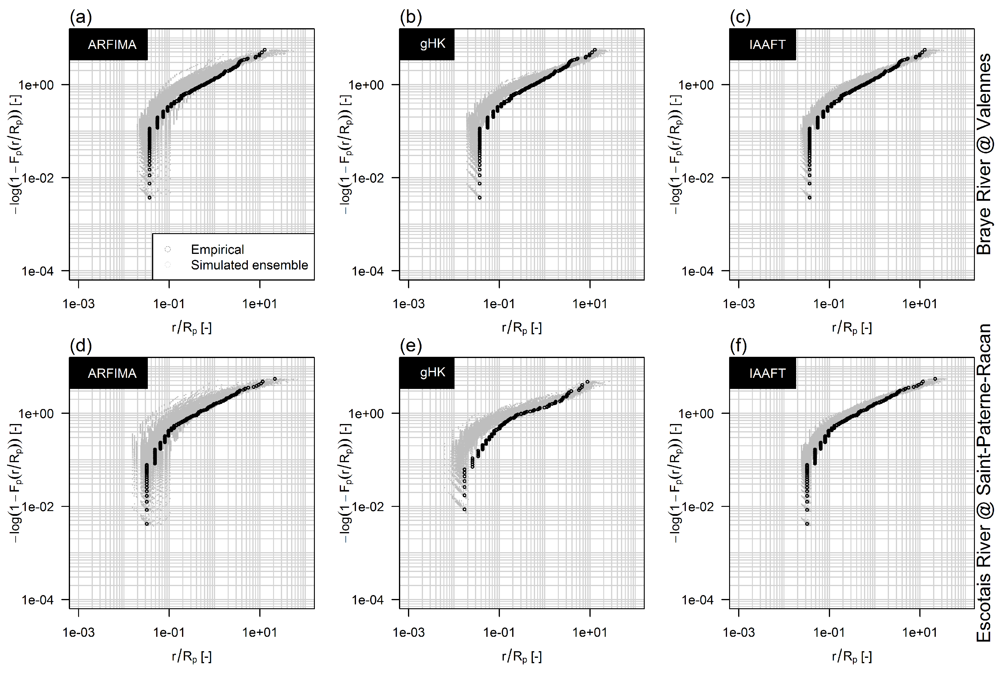
Because of computational burden, the analyses on return interval in Section 3.3 are based on the comparison of observed time series and one set of sequences of the same size simulated by each model/method. In other words, one simulated time series is considered for each observed one. The rationale is that a set of 473 simulated series gives an average picture of the return intervals resulting from the models considered, since positive and negative at-site discrepancies are smoothed out, whilst systematic biases remain. However, since we deal with return intervals of extreme events, which are a few by definition, relatively high uncertainty is expected especially for high values of H. To explore the impact of the sampling uncertainty, we selected two time series with flagged as “pristine” corresponding to 45 years of records from 1968 to 2012 for the French rivers Braye at Valennes (GRDC ID 6123220) and Escotais at Saint-Paterne-Racan (GRDC ID 6123230).
Figure 13 shows the diagrams of the negative logarithm of the survival function versus in log-log plot for the two observed series and a set of 100 series simulated by gHK, ARFIMA, and IAAFT, and 95% threshold. The diagrams show that the bias characterizes all simulated series when it does exist, thus confirming that the use of single realization for each location can provide a fair qualitative picture of the performance of each model in reproducing the observed patterns. Of course, the uncertainty increases as the threshold increases (Figures S5 and S6), and its magnitude is comparable to the inter-station variability (Figure 10, Figures S1 and S2).
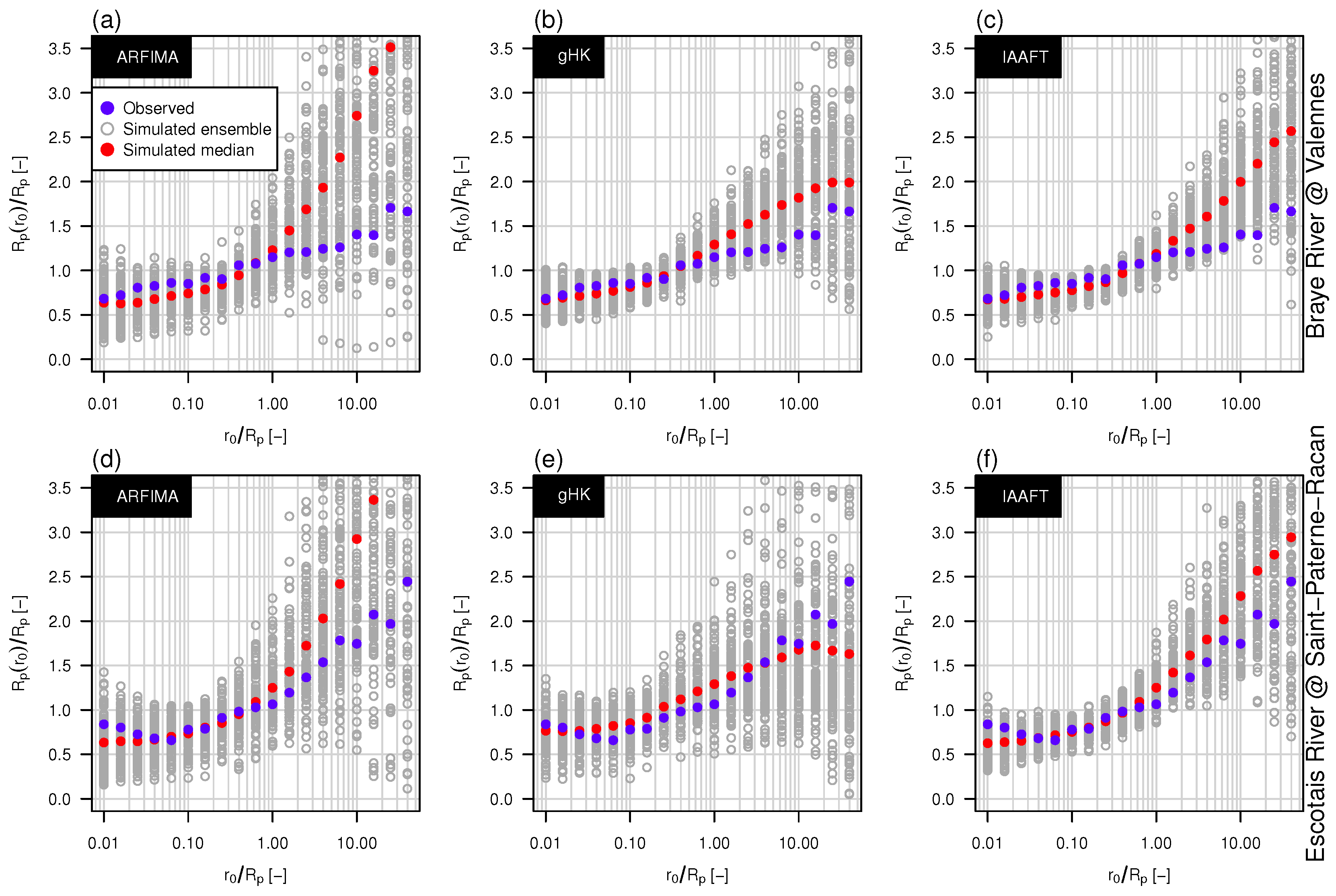
The uncertainty is even higher for the conditional return periods . Figure 14 shows the patterns of versus for the observed series, an ensemble of 100 simulated series and the corresponding median pattern. It is worth noting that the magnitude of the sampling variability is similar to that of the inter-station variability (Figure 11). In spite of the large variability, single realizations generally depart from the observed pattern when a systematic bias does exist. Therefore, this confirms the validity of the analysis in Section 3.3, but on the other side it also highlights that the size of available records might be insufficient to draw reliable conclusions on the properties of extremes. A fair communication of this uncertainty is paramount for a well-informed decision process.
3.5. The Effect of Persistence on Collective Risk
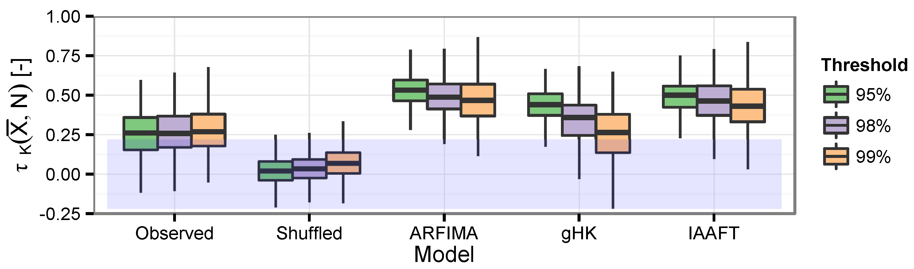
As mentioned in Section 1, a common assumption in the computation of is the independence between and N. Here, losses denote the deseasonalized flows exceeding and N is the number of such exceedances over 365-day time windows. The relationship between and N is studied by the Kendall correlation coefficient between N and the average value of the deseasonalized flow intensities . Box plots in Figure 15 show that SRD and LRD introduce significant correlation between N and . However, ARFIMA, gHK, and IAAFT tend to overestimate the strength of this relationship. Since the three methods yield similar results, and IAAFT signals differ from the observed sequences in the statistics of order higher than two, we argue that the difference should be mainly due to the temporal skewness or higher order properties, and thus to nonlinear dynamics that are not captured by linear models and can be related to multifractality/varying scaling behavior (e.g., [19,71,72]).
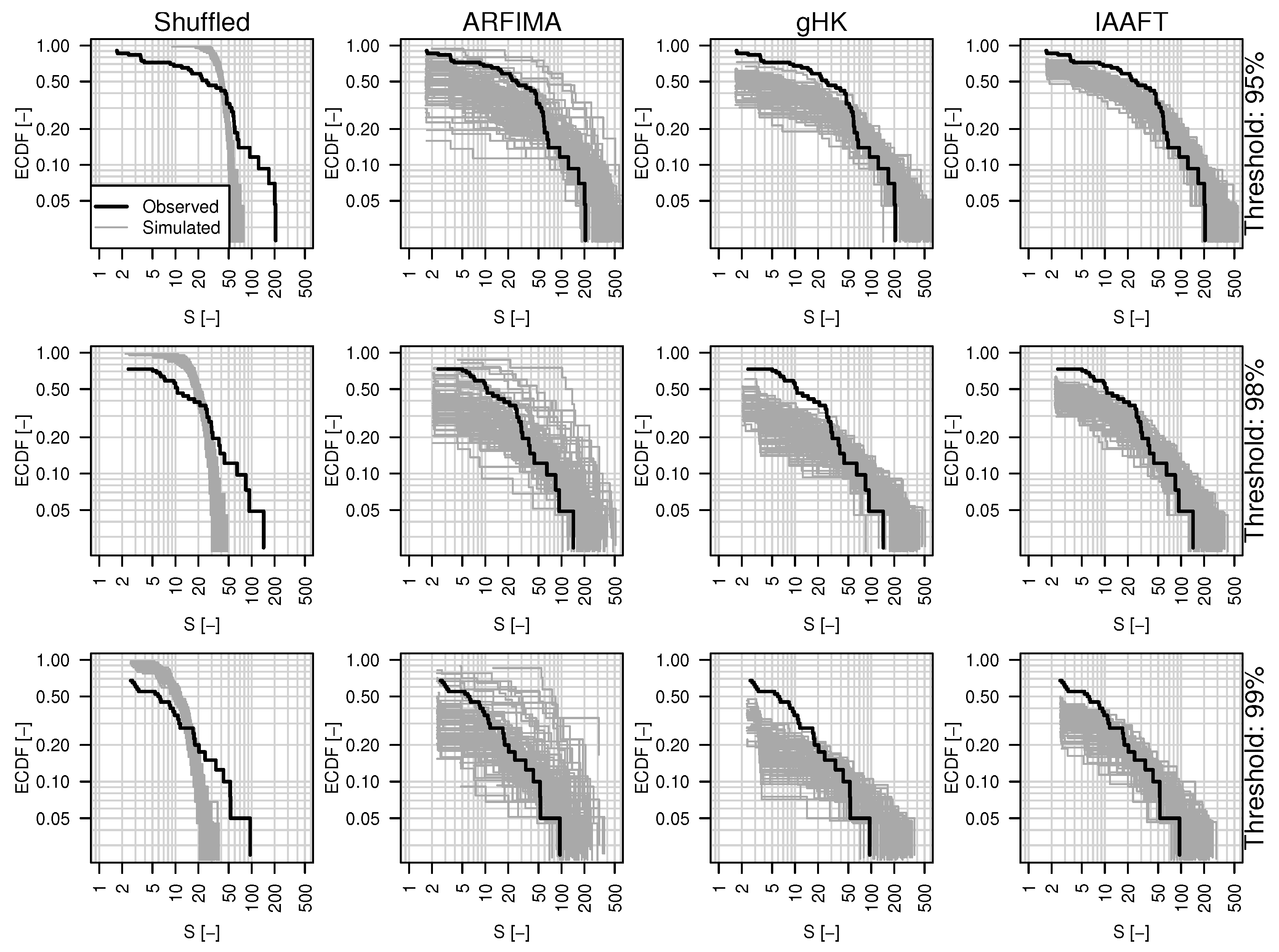
The correlation between and N also impacts on the distribution of . For example, Figure 16 shows the empirical cumulative distribution function (ECDF) of for the Escotais River time series discussed in the previous sections along with the corresponding ECDFs resulting from 100 time series simulated by ARFIMA, gHK, IAAFT, and shuffling procedure.
The agreement between autocorrelated sequences and the evident discrepancies resulting from the removal of the temporal correlation show that SRD and LRD imply both events’ clustering and the increase of the average intensity of such events. Indeed, under SRD and LRD, the distribution of exhibits a spike of probability at zero corresponding to years with no exceedances and an upper tail heavier than under independence, describing the tendency of events in flood-rich periods to be more extreme than expected under random (Poissonian) arrival dynamics. However, as mentioned above, ARFIMA, gHK, IAAFT miss some piece of information, thus resulting in expected residual discrepancies (see also Figure S7 for the case of the Braye River).
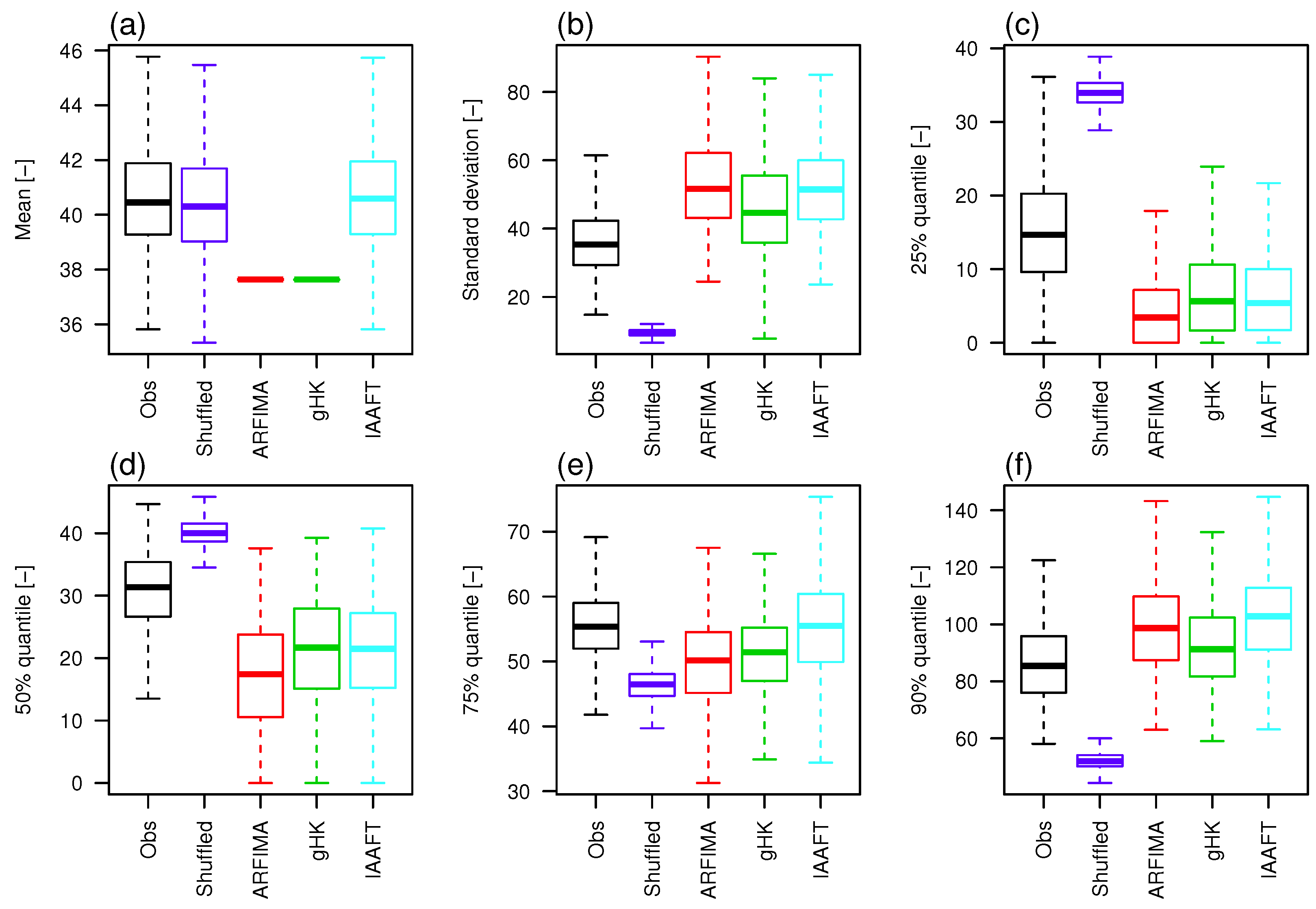
For a quantitative assessment involving the entire data set, ECDFs are summarized by a set of suitable statistics: mean, standard deviation, and four quantiles , . Figure 17 shows box plots of these summary statistics for observations, shuffled data, and data simulated by ARFIMA, gHK, IAAFT, and 95% threshold (see Figures S8 and S9 for the other thresholds). Data drawn from parametric models tend to underestimate the average of , which in turn is accurately reproduced by shuffled data and IAAFT, as these series preserve almost exactly the marginal distribution, apart from random fluctuations related to the resampling procedures. As expected, correlation has a dramatic effect on the variability (Figure 17b); ARFIMA, gHK, and IAAFT tend to overestimate the observed standard deviation of , but yield results similar to each other. Box plots of quantiles (Figure 17c–f) confirm that the patterns in Figure 16 and Figure S7 are general, and highlight that the ECDFs of shuffled data cross the ECDFs of observations and simulations around the quantile. Below this quantile, the ECDFs of shuffled data are stochastically dominated by ECDFs of observations and simulations because of the spike of probability at zero due to years with no events, while above the 75% quantile we have the opposite behavior because of the higher variability of the autocorrelated signals, which results in increased clustering and larger values.
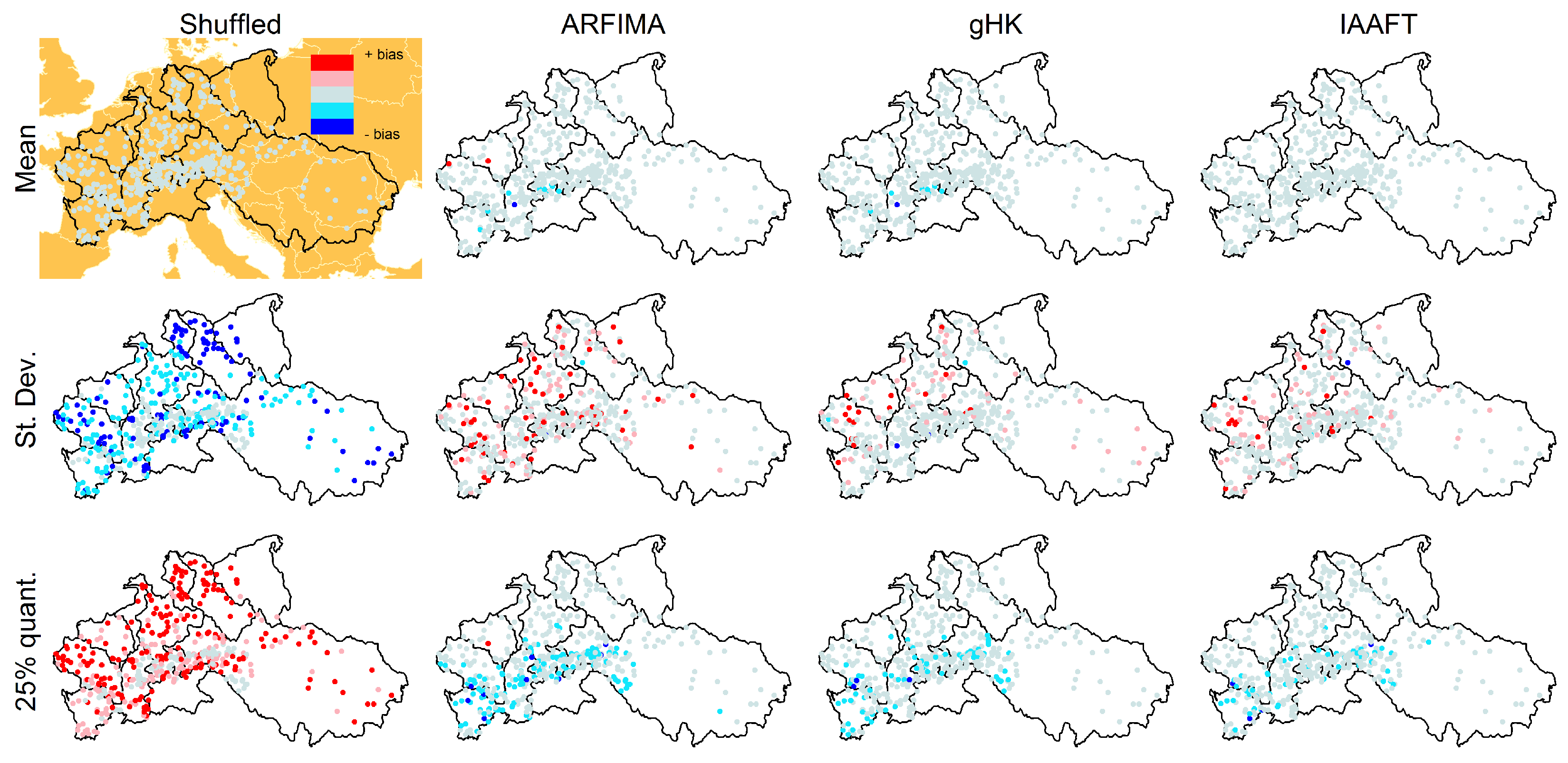
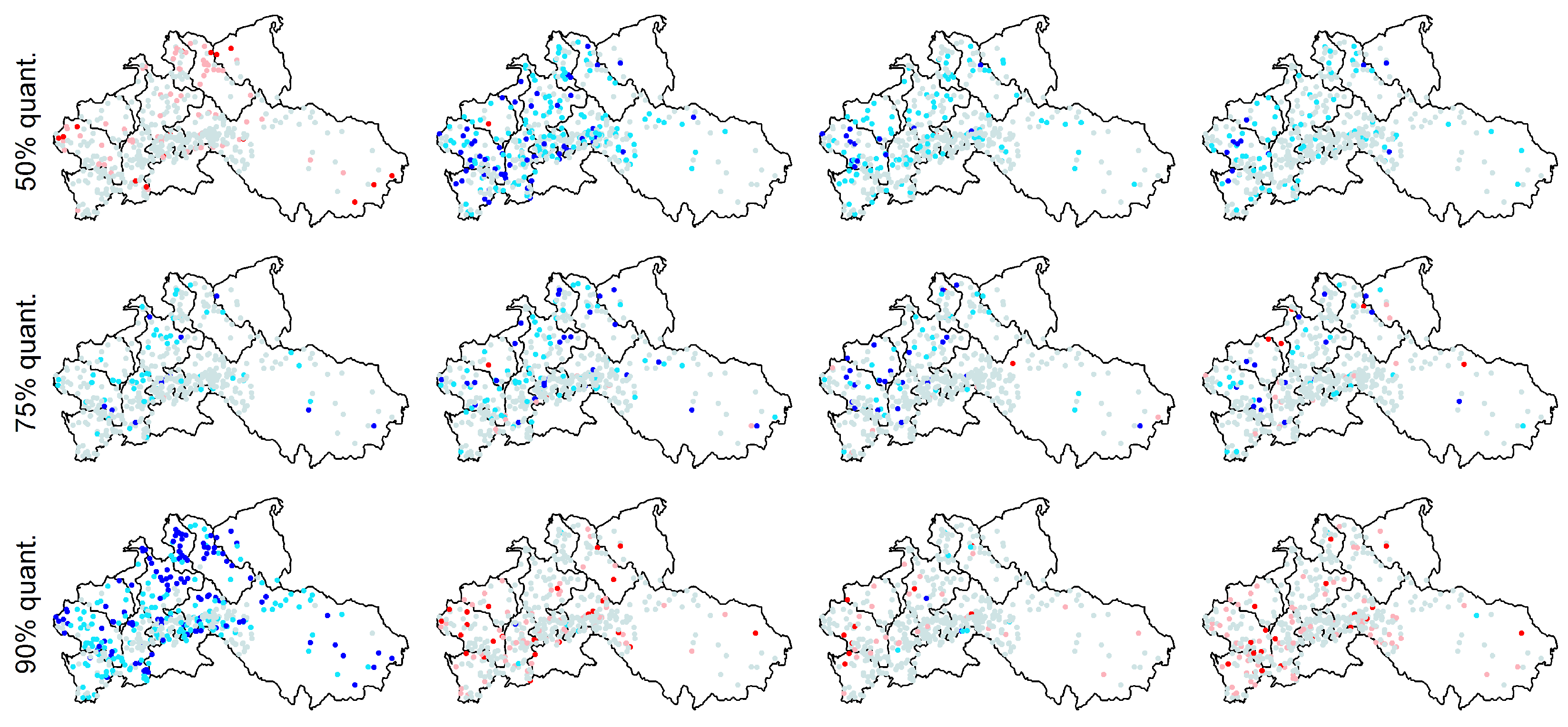
For the above summary statistics, Figure 18 shows the spatial distribution of the difference between modeled and observed values reported in Figure 17. We denote this difference as bias even though this term is not strictly correct because we simply compare the observed values with those resulting from a single simulated sequences for each location. Nonetheless, if the discrepancies are random, we expect a spatial random patterns of the differences, while we expect coherent spatial patterns if the models show a systematic bias. Figure 18 shows that ARFIMA and gHK underestimate the mean value of especially for the Alpine basins, Garonne, and Loire, thus denoting a systematic lack of fit for time series in that area. The bias of standard deviation does not show particular spatial patterns. ARFIMA, gHK, and IAAFT underestimate in the Alpine basins and Garonne. No particular spatial patterns are evident for the and bias, which is generally negative for ARFIMA, gHK, and IAAFT. These models yield unbiased or slightly positive biased results for with no specific spatial pattern. Similar results hold for the 98% and 99% thresholds (see Figures S10 and S11).
4. Conclusions
In this study, we have investigated the properties of daily stream flow fluctuations exceeding high thresholds analyzing 473 time series recorded in the major basins in Europe, and comparing the results with those corresponding to synthetic time series simulated by a set of linear models. The aim was to better understand some aspects concerning the occurrence and magnitude of extreme flow values and their relationship with the properties of the complete time series in a collective risk perspective, in order to pave the way for the development of modeling strategies based on the efficient use of all the available information and not only a limited number of extreme events. Results can be summarized as follows:
- Extending previous analyses [19] and resorting to recently proposed tools such as bias-corrected climacograms and gHK model (merging SRD and LRD), we strengthen the empirical evidence that the crossover in DFA patterns and the behavior of empirical climacograms of mean daily stream flow signals can be attributed to the interplay of SRD and LRD rather than residual seasonality as sometimes argued in the literature. This conclusion is confirmed by the results corresponding to synthetic signals showing only LRD (simulated by HK model) or SRD and LRD (simulated by ARFIMA and gHK models and the IAAFT resampling method). In particular, gHK seems to be a parsimonious, flexible and physically consistent option compared with highly-parameterized ARFIMA models. However, since all these models/methods are linear, they can reproduce flow characteristics up to the second order, thus excluding the observed temporal asymmetry, which can be measured by third-order temporal coefficient of skewness. Time irreversibility provides further evidence for nonlinearity of stream flow dynamics [73] , thus confirming by a different analysis the stream flow nonlinear behavior recognized by Kantelhardt et al. [19] by multifractal DFA. Our analyses also show that the recognition of possible LRD requires additional care and need to account for the effect of SRD, and use suitable processes as benchmark for comparisons and validations of empirical results.
- Focusing on the behavior of the return intervals between over-threshold values, our results further confirm the behavior previously highlighted by e.g., Bunde et al. [69], and Bogachev and Bunde [32] for less extensive stream flow data sets. Namely, return intervals tend to follow a sub-exponential (Weibull-like) distribution, implying a higher (smaller) probability of observing long (short) return intervals longer (shorter) than expected under independence (i.e., Poisson process with exponentially distributed inter-arrival times). Moreover, the statistics of conditional return periods (expected return intervals) show that the sequence of return intervals is no longer independent, meaning that short (long) return intervals tend to follow short (long) return intervals. This partly explains the so-called clustering of extreme events observed in many natural phenomena [69], and has important practical consequences. For example, reviewing factors influencing private flood mitigation behavior, Bubeck et al. [74] highlighted that experience with floods is often considered to have a great impact on the recognition of risk, resulting for instance in a positive relationship between individual flood risk perceptions in the Netherlands and demand for flood insurance [75]. Moreover, an important role is also played by the severity of the experienced negative consequences along with the timing of the previous experience, since it can be expected that floods experienced in the distant past have only a limited influence on individual risk perceptions and mitigation behavior later [74]. In this respect, Bubeck et al. [74] highlighted that the International Commission for the Protection of the Rhine (ICPR) estimates that flood awareness mostly diminishes within seven years after a flood and that only catastrophic disasters are remembered in the long term [76], and that flood damage is significantly lower in areas where people have recently experienced a flood event, which is attributed to a better preparedness of the population in the direct aftermath of a flood [77,78,79]. The better understanding of the causes of flood clustering is therefore paramount to set up effective mitigation strategies that are not affected by the flood risk perception related to the alternation of flood-rich and flood-poor periods.
- From a collective risk perspective, the previous remarks are further strengthened by the empirical evidence of the positive correlation of the average intensity of extreme flows and the number of events over one-year time windows, implying that years that are more active in terms of number of events tend to exhibit more extreme events also in terms of average magnitude. This behavior results in distributions of the cumulated flow (which can be seen as a proxy of the potential annual losses) characterized by a spike of probability at zero, which describes the probability of years with no events, and a heavier upper tail, which indicates a probability of more extreme annual losses larger than expected under independence. Concerning these aspects, the linear models used in this study only partly reproduce the observed behavior. In particular, since IAAFT preserves almost exactly both marginal distribution and the empirical power spectrum, we argue that nonlinearity might be the cause of the observed discrepancies between observations and simulations. However, other factors such as river training, dam building and operation, and other anthropogenic interventions cannot be excluded. Therefore, we suggest repeating the analyses reported in this study on data sets of (reasonably) natural stream flow records such as those of the U.S. Geological Survey Hydro-Climatic Data Network (HCDN-2009; [80]).
Supplementary Materials
The following are available online at www.mdpi.com/2073-4441/8/4/152/s1, Table S1 (List of stream gage stations used in the analyses), Figures S1–S11.
Acknowledgments
This work was supported by the Engineering and Physical Sciences Research Council (EPSRC) grant EP/K013513/1 “Flood MEMORY: Multi-Event Modelling of Risk & recoverY”, and Willis Research Network. We acknowledge the Global Runoff Data Centre (GRDC; Federal Institute of Hydrology (BfG), Koblenz, Germany) for providing the daily river flow data. The authors wish to thank three anonymous reviewers for their constructive remarks and criticisms that helped improve the original manuscript. The analyses were performed in R [81] by using the contributed packages fArma [82], FGN [83], fracdiff [84], fractal [85], ltsa [68], and muhaz [86].
Author Contributions
Francesco Serinaldi and Chris G. Kilsby conceived and wrote the paper; Francesco Serinaldi analyzed the data.
Conflicts of Interest
The authors declare no conflict of interest.
Appendix
The gHK parameters can be estimated following a two-stage procedure based on climacogram [17]. It consists of minimizing two fitting errors:
where Δ denotes the temporal resolution of the observed discrete process (one day, here), is the empirical climacogram estimated from the data, and is the expected one estimated from the model
in which γ is the gHK climacogram
with . The LSV (least square based on variance) method proposed by Tyralis and Koutsoyiannis [12] for HK is used to obtain preliminary estimates of λ and , which are used as initial values to minimize in Equation (A1); finally, (Equation (A2)) is minimized for fine tuning [17].
References
- Mudelsee, M.; Börngen, M.; Tetzlaff, G.; Grünewald, U. Extreme floods in central Europe over the past 500 years: Role of cyclone pathway “Zugstrasse Vb”. J. Geophys. Res. Atmos. 2004, 109. [Google Scholar] [CrossRef]
- Glaser, R.; Riemann, D.; Schönbein, J.; Barriendos, M.; Brázdil, R.; Bertolin, C.; Camuffo, D.; Deutsch, M.; Dobrovolný, P.; van Engelen, A.; et al. The variability of European floods since AD 1500. Clim. Chang. 2010, 101, 235–256. [Google Scholar] [CrossRef]
- Hall, J.; Arheimer, B.; Borga, M.; Brázdil, R.; Claps, P.; Kiss, A.; Kjeldsen, T.R.; Kriaučiūnienė, J.; Kundzewicz, Z.W.; Lang, M.; et al. Understanding flood regime changes in Europe: A state-of-the-art assessment. Hydrol. Earth Syst. Sci. 2014, 18, 2735–2772. [Google Scholar] [CrossRef] [Green Version]
- Barredo, J.I. Major flood disasters in Europe: 1950–2005. Nat. Hazards 2007, 42, 125–148. [Google Scholar] [CrossRef]
- Kundzewicz, Z.W.; Pinskwar, I.; Brakenridge, G.R. Large floods in Europe, 1985–2009. Hydrol. Sci. J. 2013, 58, 1–7. [Google Scholar] [CrossRef]
- Montanari, A. Hydrology of the Po River: Looking for changing patterns in river discharge. Hydrol. Earth Syst. Sci. 2012, 16, 3739–3747. [Google Scholar] [CrossRef]
- Hurst, H.E. Long–term storage capacity of reservoirs. Trans. Am. Soc. Civil Eng. 1951, 116, 770–808. [Google Scholar]
- Taqqu, M.S.; Teverovsky, V.; Willinger, W. Estimators for long-range dependence: An empirical study. Fractals 1995, 3, 785–798. [Google Scholar] [CrossRef]
- Malamud, B.D.; Turcotte, D.L. Self-affine time series: Measures of weak and strong persistence. J. Stat. Plan. Inference 1999, 80, 173–196. [Google Scholar]
- Kantelhardt, J.W.; Zschiegner, S.A.; Koscielny-Bunde, E.; Havlin, S.; Bunde, A.; Stanley, H.E. Multifractal detrended fluctuation analysis of nonstationary time series. Phys. A Stat. Mech. Appl. 2002, 316, 87–114. [Google Scholar] [CrossRef]
- Serinaldi, F. Use and misuse of some Hurst parameter estimators applied to stationary and non-stationary financial time series. Phys. A Stat. Mech. Appl. 2010, 389, 2770–2781. [Google Scholar] [CrossRef]
- Tyralis, H.; Koutsoyiannis, D. Simultaneous estimation of the parameters of the Hurst-Kolmogorov stochastic process. Stoch. Environ. Res. Risk Assess. 2011, 25, 21–33. [Google Scholar] [CrossRef]
- Mandelbrot, B.B.; Ness, J.W.V. Fractional Brownian Motions, Fractional Noises and Applications. SIAM Rev. 1968, 10, 422–437. [Google Scholar] [CrossRef]
- Hosking, J.R.M. Fractional differencing. Biometrika 1981, 68, 165–176. [Google Scholar] [CrossRef]
- Beran, J. Statistics for Long-Memory Processes; Chapman & Hall/CRC Monographs on Statistics & Applied Probability: Taylor & Francis: Boca Raton, FL, USA, 1994. [Google Scholar]
- Hipel, K.W.; McLeod, A.I. Time Series Modelling of Water Resources and Environmental Systems; Developments in Water Science, Elsevier Science: Amsterdam, The Netherlands, 1994. [Google Scholar]
- Dimitriadis, P.; Koutsoyiannis, D. Climacogram versus autocovariance and power spectrum in stochastic modelling for Markovian and Hurst-Kolmogorov processes. Stoch. Environ. Res. Risk Assess. 2015, 29, 1649–1669. [Google Scholar] [CrossRef]
- Kantelhardt, J.W.; Rybski, D.; Zschiegner, S.A.; Braun, P.; Koscielny-Bunde, E.; Livina, V.; Havlin, S.; Bunde, A. Multifractality of river runoff and precipitation: Comparison of fluctuation analysis and wavelet methods. Phys. A Stat. Mech. Appl. 2003, 330, 240–245. [Google Scholar] [CrossRef]
- Kantelhardt, J.W.; Koscielny-Bunde, E.; Rybski, D.; Braun, P.; Bunde, A.; Havlin, S. Long-term persistence and multifractality of precipitation and river runoff records. J. Geophys. Res. Atmos. 2006, 111. [Google Scholar] [CrossRef]
- Rao, A.; Bhattacharya, D. Effect of Short-Term Memory on Hurst Phenomenon. J. Hydrol. Eng. 2001, 6, 125–131. [Google Scholar] [CrossRef]
- Koutsoyiannis, D.; Montanari, A. Statistical analysis of hydroclimatic time series: Uncertainty and insights. Water Resour. Res. 2007, 43. [Google Scholar] [CrossRef]
- Wang, W.; van Gelder, P.H.A.J.M.; Vrijling, J.K.; Chen, X. Detecting long-memory: Monte Carlo simulations and application to daily streamflow processes. Hydrol. Earth Syst. Sci. 2007, 11, 851–862. [Google Scholar] [CrossRef]
- Montanari, A.; Rosso, R.; Taqqu, M.S. Fractionally differenced ARIMA models applied to hydrologic time series: Identification, estimation, and simulation. Water Resour. Res. 1997, 33, 1035–1044. [Google Scholar] [CrossRef]
- Montanari, A.; Longoni, M.; Rosso, R. A seasonal long-memory stochastic model for the simulation of daily river flows. Phys. Chem. Earth B Hydrol. Oceans Atmos. 1999, 24, 319–324. [Google Scholar] [CrossRef]
- Montanari, A.; Rosso, R.; Taqqu, M.S. A seasonal fractional ARIMA model applied to the Nile River monthly flows at Aswan. Water Resour. Res. 2000, 36, 1249–1259. [Google Scholar] [CrossRef]
- Elek, P.; Márkus, L. A long range dependent model with nonlinear innovations for simulating daily river flows. Nat. Hazards Earth Syst. Sci. 2004, 4, 277–283. [Google Scholar] [CrossRef]
- Eichner, J.F.; Kantelhardt, J.W.; Bunde, A.; Havlin, S. Extreme value statistics in records with long-term persistence. Phys. Rev. E 2006, 73. [Google Scholar] [CrossRef] [PubMed]
- Eichner, J.F.; Kantelhardt, J.W.; Bunde, A.; Havlin, S. Statistics of return intervals in long-term correlated records. Phys. Rev. E 2007, 75, 011128. [Google Scholar] [CrossRef] [PubMed]
- Eichner, J.F.; Kantelhardt, J.W.; Bunde, A.; Havlin, S. The Statistics of Return Intervals, Maxima, and Centennial Events Under the Influence of Long-Term Correlations. In In Extremis; Kropp, J., Schellnhuber, H.J., Eds.; Springer: Berlin, Geramny; Heidelberg, Germany, 2011; pp. 2–43. [Google Scholar]
- Bogachev, M.I.; Eichner, J.F.; Bunde, A. Effect of nonlinear correlations on the statistics of return intervals in multifractal data sets. Phys. Rev. Lett. 2007, 99. [Google Scholar] [CrossRef] [PubMed]
- Bogachev, M.I.; Eichner, J.F.; Bunde, A. The effects of multifractality on the statistics of return intervals. Eur. Phys. J. Spec. Top. 2008, 161, 181–193. [Google Scholar] [CrossRef]
- Bogachev, M.I.; Bunde, A. Universality in the precipitation and river runoff. Europhys. Lett. 2012, 97. [Google Scholar] [CrossRef]
- Matsoukas, C.; Islam, S.; Rodriguez-Iturbe, I. Detrended fluctuation analysis of rainfall and streamflow time series. J. Geophys. Res. Atmos. 2000, 105, 29165–29172. [Google Scholar] [CrossRef]
- Labat, D.; Masbou, J.; Beaulieu, E.; Mangin, A. Scaling behavior of the fluctuations in stream flow at the outlet of karstic watersheds, France. J. Hydrol. 2011, 410, 162–168. [Google Scholar] [CrossRef]
- Serinaldi, F.; Zunino, L.; Rosso, O.A. Complexity-entropy analysis of daily stream flow time series in the continental United States. Stoch. Environ. Res. Risk Assess. 2014, 28, 1685–1708. [Google Scholar] [CrossRef]
- Szolgayova, E.; Laaha, G.; Blöschl, G.; Bucher, C. Factors influencing long range dependence in streamflow of European rivers. Hydrol. Processes 2014, 28, 1573–1586. [Google Scholar] [CrossRef]
- Kaas, R.; Goovaerts, M.; Dhaene, J.; Denuit, M. Modern Actuarial Risk Theory: Using R; Springer Science & Business Media: New York, NY, USA, 2008; Volume 128. [Google Scholar]
- Cleveland, W.S.; Devlin, S.J. Locally-Weighted Regression: An Approach to Regression Analysis by Local Fitting. J. Am. Stat. Assoc. 1988, 83, 596–610. [Google Scholar] [CrossRef]
- Cleveland, R.B.; Cleveland, W.S.; McRae, J.E.; Terpenning, I. STL: A seasonal-trend decomposition procedure based on loess. J. Off. Stat. 1990, 6, 3–73. [Google Scholar]
- Bogachev, M.I.; Bunde, A. Improved risk estimation in multifractal records: Application to the value at risk in finance. Phys. Rev. E 2009, 80. [Google Scholar] [CrossRef] [PubMed]
- Bogachev, M.I.; Bunde, A. On the occurrence and predictability of overloads in telecommunication networks. Europhys. Lett. 2009, 86. [Google Scholar] [CrossRef]
- Hosking, J.R.M. Modeling persistence in hydrological time series using fractional differencing. Water Resour. Res. 1984, 20, 1898–1908. [Google Scholar]
- Mandelbrot, B.B.; Wallis, J.R. Computer experiments with fractional Gaussian noises: Part 1, averages and variances. Water Resour. Res. 1969, 5, 228–241. [Google Scholar] [CrossRef]
- Mandelbrot, B.B.; Wallis, J.R. Computer experiments with fractional Gaussian noises: Part 2, rescaled ranges and spectra. Water Resour. Res. 1969, 5, 242–259. [Google Scholar] [CrossRef]
- Mandelbrot, B.B.; Wallis, J.R. Computer experiments with fractional Gaussian noises: Part 3, mathematical appendix. Water Resour. Res. 1969, 5, 260–267. [Google Scholar] [CrossRef]
- Koutsoyiannis, D. The Hurst phenomenon and fractional Gaussian noise made easy. Hydrol. Sci. J. 2002, 47, 573–595. [Google Scholar] [CrossRef]
- Koutsoyiannis, D. A random walk on water. Hydrol. Earth Syst. Sci. 2010, 14, 585–601. [Google Scholar] [CrossRef]
- Koutsoyiannis, D. Hurst-Kolmogorov Dynamics and Uncertainty. J. Am. Water Resour. Assoc. 2011, 47, 481–495. [Google Scholar] [CrossRef]
- Schreiber, T.; Schmitz, A. Improved Surrogate Data for Nonlinearity Tests. Phys. Rev. Lett. 1996, 77, 635–638. [Google Scholar] [CrossRef] [PubMed]
- Kugiumtzis, D. Test your surrogate data before you test for nonlinearity. Phys. Rev. E 1999, 60, 2808–2816. [Google Scholar] [CrossRef]
- Schreiber, T.; Schmitz, A. Surrogate time series. Phys. D Nonlinear Phenom. 2000, 142, 346–382. [Google Scholar] [CrossRef]
- Venema, V.; Ament, F.; Simmer, C. A Stochastic Iterative Amplitude Adjusted Fourier Transform algorithm with improved accuracy. Nonlinear Processes Geophys. 2006, 13, 321–328. [Google Scholar] [CrossRef]
- Venema, V.; Bachner, S.; Rust, H.W.; Simmer, C. Statistical characteristics of surrogate data based on geophysical measurements. Nonlinear Processes Geophys. 2006, 13, 449–466. [Google Scholar] [CrossRef]
- Koutsoyiannis, D. Generic and parsimonious stochastic modelling for hydrology and beyond. Hydrol. Sci. J. 2016, 61, 225–244. [Google Scholar] [CrossRef]
- Koutsoyiannis, D. Hydrology and change. Hydrol. Sci. J. 2013, 58, 1177–1197. [Google Scholar] [CrossRef]
- Franzke, C. A novel method to test for significant trends in extreme values in serially dependent time series. Geophys. Res. Lett. 2013, 40, 1391–1395. [Google Scholar] [CrossRef]
- Livina, V.N.; Ashkenazy, Y.; Braun, P.; Monetti, R.; Bunde, A.; Havlin, S. Nonlinear volatility of river flux fluctuations. Phys. Rev. E 2003, 67. [Google Scholar] [CrossRef] [PubMed]
- Beran, J. A Test of Location for Data with Slowly Decaying Serial Correlations. Biometrika 1989, 76, 261–269. [Google Scholar] [CrossRef]
- Peng, C.K.; Buldyrev, S.V.; Havlin, S.; Simmons, M.; Stanley, H.E.; Goldberger, A.L. Mosaic organization of DNA nucleotides. Phys. Rev. E 1994, 49, 1685–1689. [Google Scholar] [CrossRef]
- Kantelhardt, J.W. Chapter Fractal and Multifractal Time Series. In Mathematics of Complexity and Dynamical Systems; Springer New York: New York, NY, USA, 2011; pp. 463–487. [Google Scholar]
- Moreira, I.G.; Kamphorst Leal da Silva, I.; Kamphorst, S.O. On the fractal dimension of self-affine profiles. J. Phys. A 1994, 27, 8079–8089. [Google Scholar] [CrossRef]
- Montanari, A.; Taqqu, M.S.; Teverovsky, V. Estimating long-range dependence in the presence of periodicity: An empirical study. Math. Comput. Model. 1999, 29, 217–228. [Google Scholar] [CrossRef]
- Marković, D.; Koch, M. Sensitivity of Hurst parameter estimation to periodic signals in time series and filtering approaches. Geophys. Res. Lett. 2005, 32. [Google Scholar] [CrossRef]
- Ludescher, J.; Bogachev, M.I.; Kantelhardt, J.W.; Schumann, A.Y.; Bunde, A. On spurious and corrupted multifractality: The effects of additive noise, short-term memory and periodic trends. Phys. A Stat. Mech. Appl. 2011, 390, 2480–2490. [Google Scholar] [CrossRef]
- Zhang, Q.; Zhou, Y.; Singh, V.P.; Chen, Y.D. Comparison of detrending methods for fluctuation analysis in hydrology. J. Hydrol. 2011, 400, 121–132. [Google Scholar] [CrossRef]
- Markonis, Y.; Koutsoyiannis, D. Climatic variability over time scales spanning nine orders of magnitude: Connecting Milankovitch cycles with Hurst-Kolmogorov dynamics. Surv. Geophys. 2013, 34, 181–207. [Google Scholar] [CrossRef]
- McLeod, A.I.; Hipel, K.W. Preservation of the rescaled adjusted range: 1. A reassessment of the Hurst Phenomenon. Water Resour. Res. 1978, 14, 491–508. [Google Scholar] [CrossRef]
- McLeod, A.I.; Yu, H.; Krougly, Z.L. Algorithms for Linear Time Series Analysis: With R Package. J. Stat. Softw. 2007, 23, 1–26. [Google Scholar] [CrossRef]
- Bunde, A.; Eichner, J.F.; Kantelhardt, J.W.; Havlin, S. Long-term memory: A natural mechanism for the clustering of extreme events and anomalous residual times in climate records. Phys. Rev. Lett. 2005, 94. [Google Scholar] [CrossRef] [PubMed]
- Bogachev, M.I.; Bunde, A. On the predictability of extreme events in records with linear and nonlinear long-range memory: Efficiency and noise robustness. Phys. A Stat. Mech. Appl. 2011, 390, 2240–2250. [Google Scholar] [CrossRef]
- Ashkenazy, Y.; Baker, D.R.; Gildor, H.; Havlin, S. Nonlinearity and multifractality of climate change in the past 420,000 years. Geophys. Res. Lett. 2003, 30. [Google Scholar] [CrossRef]
- Markonis, Y.; Koutsoyiannis, D. Scale-dependence of persistence in precipitation records. Nat. Clim. Chang. 2015, in press. [Google Scholar] [CrossRef]
- Serinaldi, F.; Kilsby, C.G. Irreversibility and complex network behavior of stream flow fluctuations. Phys. A Stat. Mech. Appl. 2016, 450, 585–600. [Google Scholar] [CrossRef]
- Bubeck, P.; Botzen, W.J.W.; Aerts, J.C.J.H. A review of risk perceptions and other factors that influence flood mitigation behavior. Risk Anal. 2012, 32, 1481–1495. [Google Scholar] [CrossRef] [PubMed] [Green Version]
- Botzen, W.J.W.; van Den Bergh, J.C.J.M. Monetary valuation of insurance against flood risk under climate change. Int. Econ. Rev. 2012, 53, 1005–1026. [Google Scholar] [CrossRef]
- Egli, T.; Wehner, K.; International Commission for the Protection of the Rhine. Non Structural Flood Plain Management: Measures and Their Effectiveness; International Commission for the Protection of the Rhine: Koblenz, Germany, 2002. [Google Scholar]
- Engel, H. The flood events of 1993/1994 and 1995 in the Rhine River basin. In Destructive Water: Water-Caused Natural Disasters, Their Abatement and Control; Leavesly, G.H., Lins, H.F., Nobilis, F., Parker, R.S., Schneider, V.R., van der Ven, F.H.M., Eds.; IAHS-AISH Publication No. 239; IAHS Press: Wallingford, UK, 1997; pp. 21–32. [Google Scholar]
- Wind, H.G.; Nierop, T.M.; de Blois, C.J.; de Kok, J.L. Analysis of flood damages from the 1993 and 1995 Meuse Floods. Water Resour. Res. 1999, 35, 3459–3465. [Google Scholar] [CrossRef]
- Bubeck, P.; Botzen, W.J.W.; Kreibich, H.; Aerts, J.C.J.H. Long-term development and effectiveness of private flood mitigation measures: An analysis for the German part of the river Rhine. Nat. Hazards Earth Syst. Sci. 2012, 12, 3507–3518. [Google Scholar] [CrossRef] [Green Version]
- Lins, H. Hydro-Climatic Data Network 2009 (HCDN-2009); U.S. Geological Survey Fact Sheet 2012-3047; U.S. Geological Survey: Reston, VA, USA, 2012.
- R Development Core Team. R: A Language and Environment for Statistical Computing; R Foundation for Statistical Computing: Vienna, Austria, 2014. [Google Scholar]
- Wuertz, D. fArma: ARMA Time Series Modelling; R Package Version 3010.79; Rmetrics: Zurich, Switzerland, 2013. [Google Scholar]
- McLeod, A.I.; Veenstra, J. FGN: Fractional Gaussian Noise, Estimation and Simulation; R Package Version 2.0; Rmetrics: Zurich, Switzerland, 2012. [Google Scholar]
- Fraley, C. fracdiff: Fractionally Differenced ARIMA aka ARFIMA(p,d,q) Models; R Package Version 1.4-2 (S original by Chris Fraley and U.Washington and Seattle. R port by Fritz Leisch at TU Wien; since 2003-12: Martin Maechler; fdGPH and fdSperio and etc. by Valderio Reisen and Artur Lemonte); Rmetrics: Zurich, Switzerland, 2012. [Google Scholar]
- Constantine, W.; Percival, D. fractal: Fractal Time Series Modeling and Analysis; R Package Version 2.0-0; Rmetrics: Zurich, Switzerland, 2014. [Google Scholar]
- Hess, K. muhaz: Hazard Function Estimation in Survival Analysis; R Package Version 1.2.5 (S original by Kenneth Hess and R port by R. Gentleman); Rmetrics: Zurich, Switzerland, 2010. [Google Scholar]
Figure 1.
Map showing the location of the 473 stations included in this study.
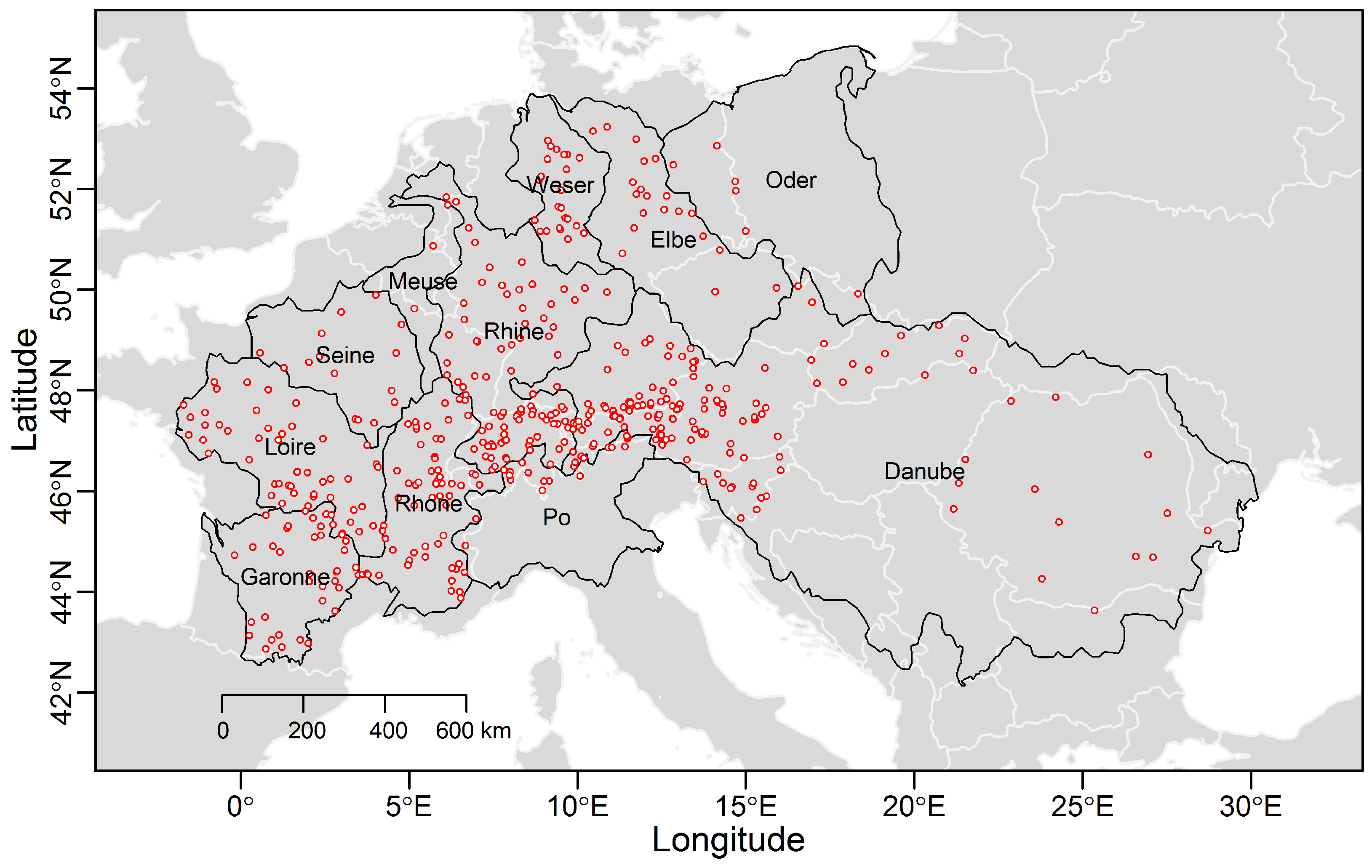
Figure 2.
(a) Time series of the number and percentage of stations available in a given year (out of 473); (b) Histogram of the record length for the 473 stations.
Figure 2.
(a) Time series of the number and percentage of stations available in a given year (out of 473); (b) Histogram of the record length for the 473 stations.

Figure 3.
Subsample of normalized and deseasonalized stream flow fluctuations for the Elbe River at Magdeburg-Strombruecke (GRDC ID 6340180) along with samples simulated by ARFIMA, HK, gHK and IAAFT. and denote HK sequences with H parameter estimated by ML and DFA, respectively (see text for further details).

Figure 4.
(a) Coefficient of temporal skewness of normalized and deseasonalized stream flow fluctuations for the Elbe River at Magdeburg-Strombruecke at several lags; (b) Magnification of the first 50 lags.
Figure 4.
(a) Coefficient of temporal skewness of normalized and deseasonalized stream flow fluctuations for the Elbe River at Magdeburg-Strombruecke at several lags; (b) Magnification of the first 50 lags.
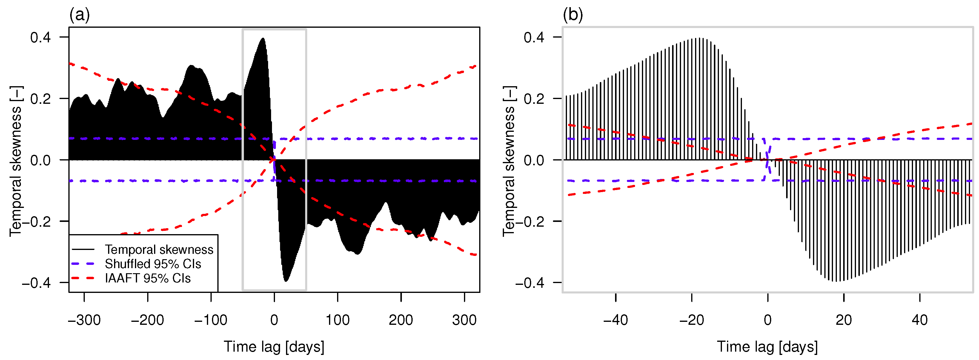
Figure 5.
Example of climacograms of observed and simulated series for the Elbe River at Magdeburg-Strombruecke. Each panel shows empirical climacograms (circles) corresponding to the observed series (a) and one example series simulated by ARFIMA (b); HK (c,d); gHK (e); and IAAFT (f). Each panel also shows the biased corrected theoretical climacograms for the first-order autoregressive AR(1) model, HK, and gHK fitted on the observed series.
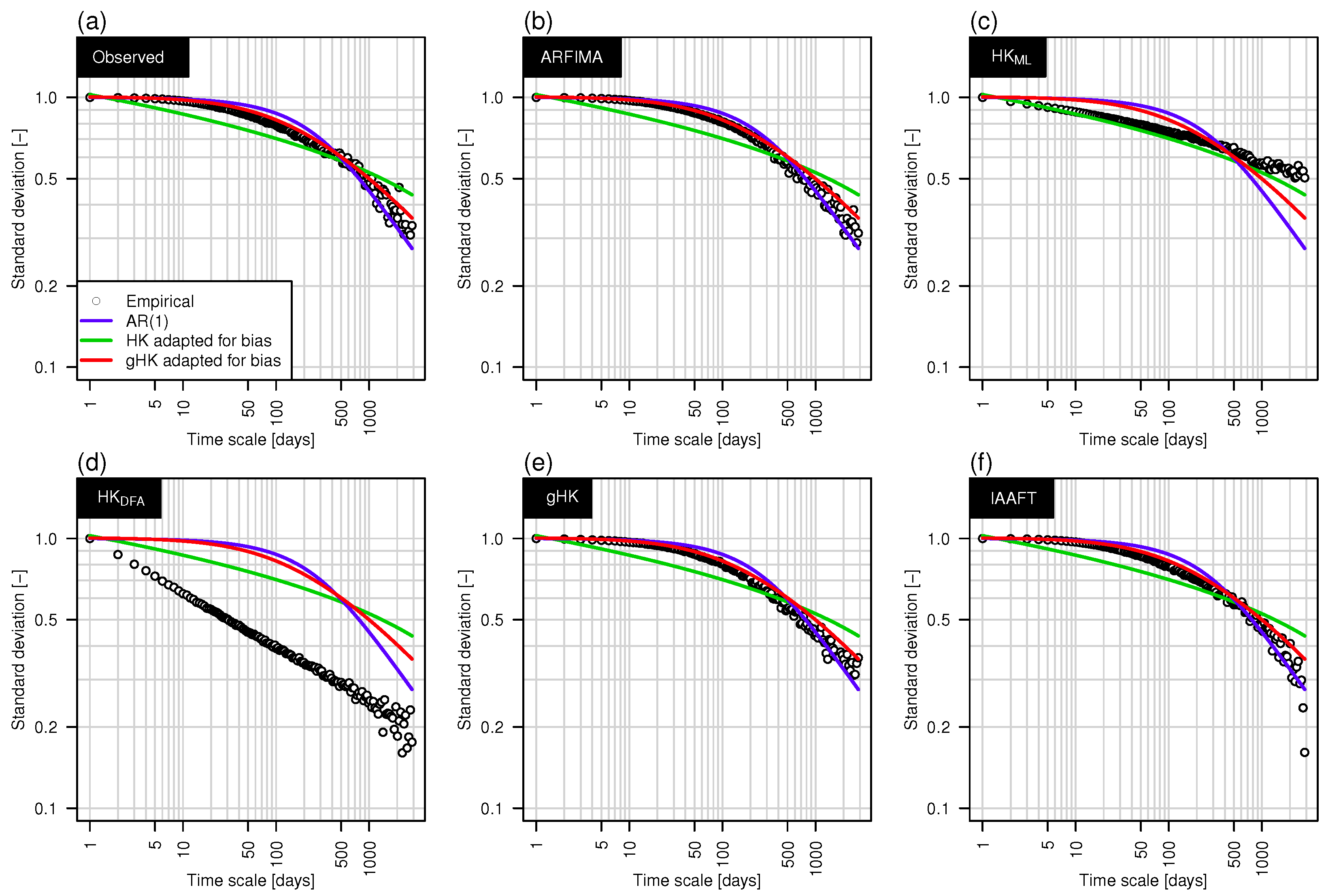
Figure 6.
Variance fluctuation functions of the 473 flow series versus the corresponding aggregation time scales k for the observed series (a) and sequences with the same length simulated by ARFIMA (b); HK (c,d); gHK (e); and IAAFT (f).
Figure 6.
Variance fluctuation functions of the 473 flow series versus the corresponding aggregation time scales k for the observed series (a) and sequences with the same length simulated by ARFIMA (b); HK (c,d); gHK (e); and IAAFT (f).

Figure 7.
Box plots of the slopes of the functions shown in Figure 6 computed for and to highlight the scaling crossover at the time scale .
Figure 7.
Box plots of the slopes of the functions shown in Figure 6 computed for and to highlight the scaling crossover at the time scale .
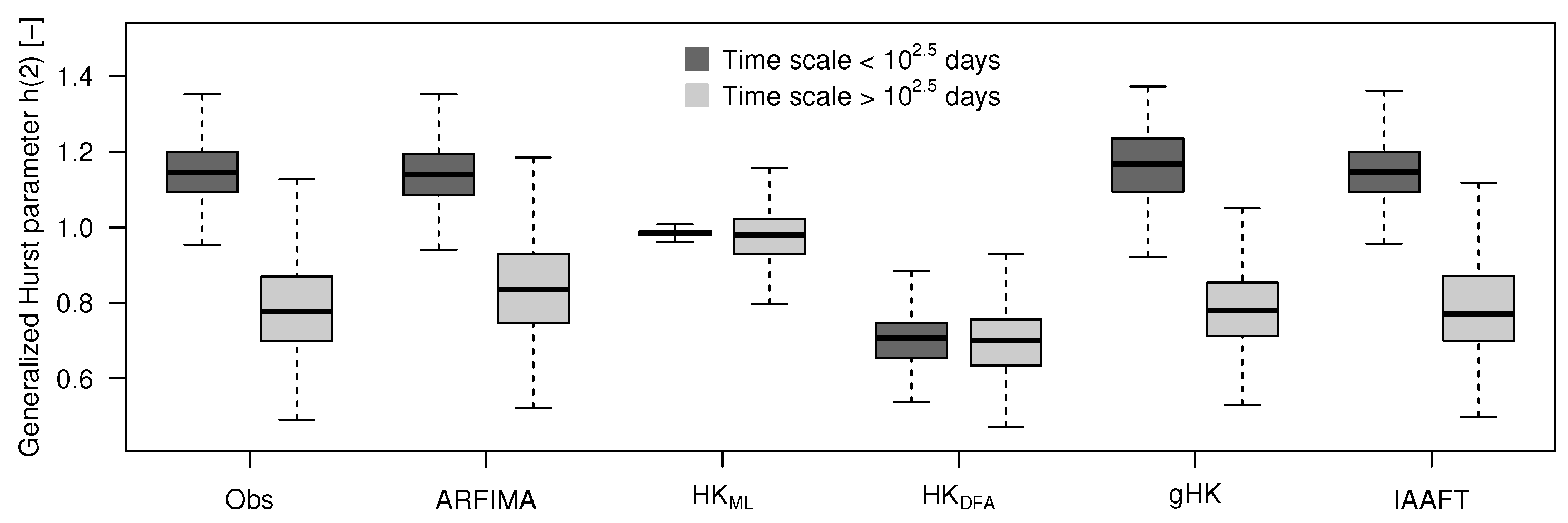
Figure 8.
H estimates by gHK, DFA, and ARFIMA: Histograms (main diagonal of panels); pairwise scatter plots and values (upper triangular matrix of panels); and spatial distribution (lower triangular matrix of panels).
Figure 8.
H estimates by gHK, DFA, and ARFIMA: Histograms (main diagonal of panels); pairwise scatter plots and values (upper triangular matrix of panels); and spatial distribution (lower triangular matrix of panels).
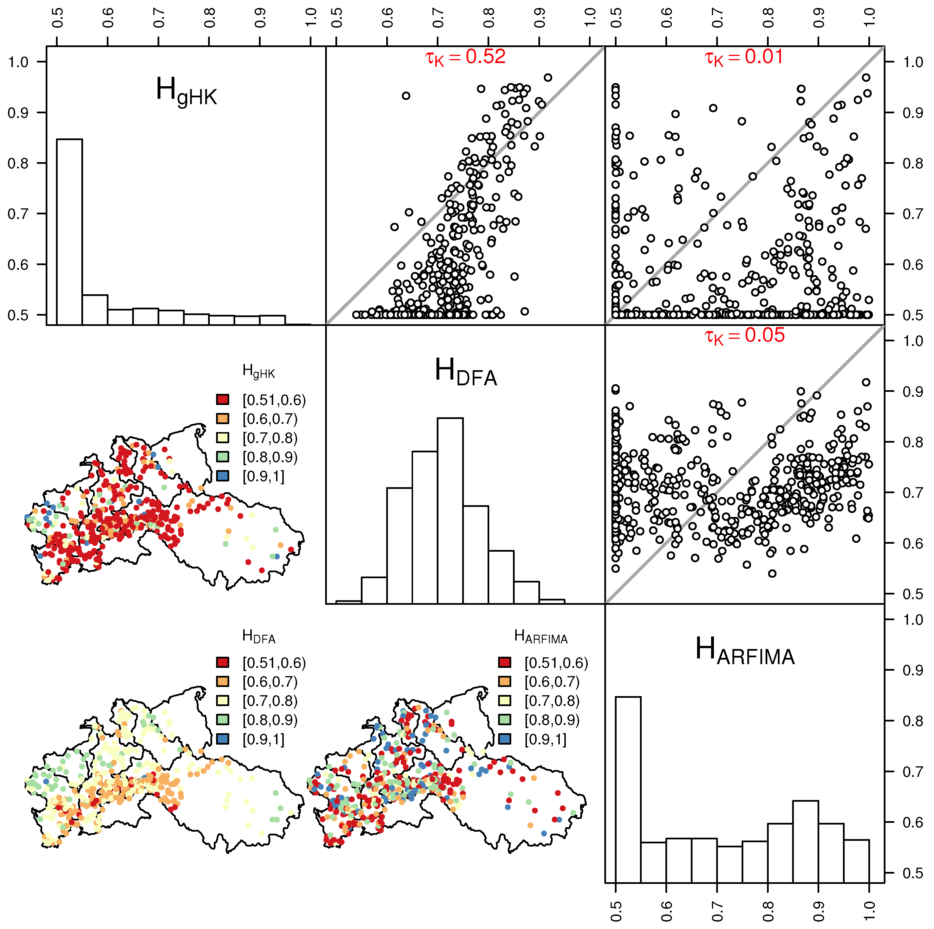
Figure 9.
Estimates of gHK parameters , λ, and q: Histograms (main diagonal of panels); pairwise scatter plots, LOESS smoothing curves (red lines), and values (upper triangular matrix of panels); and spatial distribution (lower triangular matrix of panels).
Figure 9.
Estimates of gHK parameters , λ, and q: Histograms (main diagonal of panels); pairwise scatter plots, LOESS smoothing curves (red lines), and values (upper triangular matrix of panels); and spatial distribution (lower triangular matrix of panels).
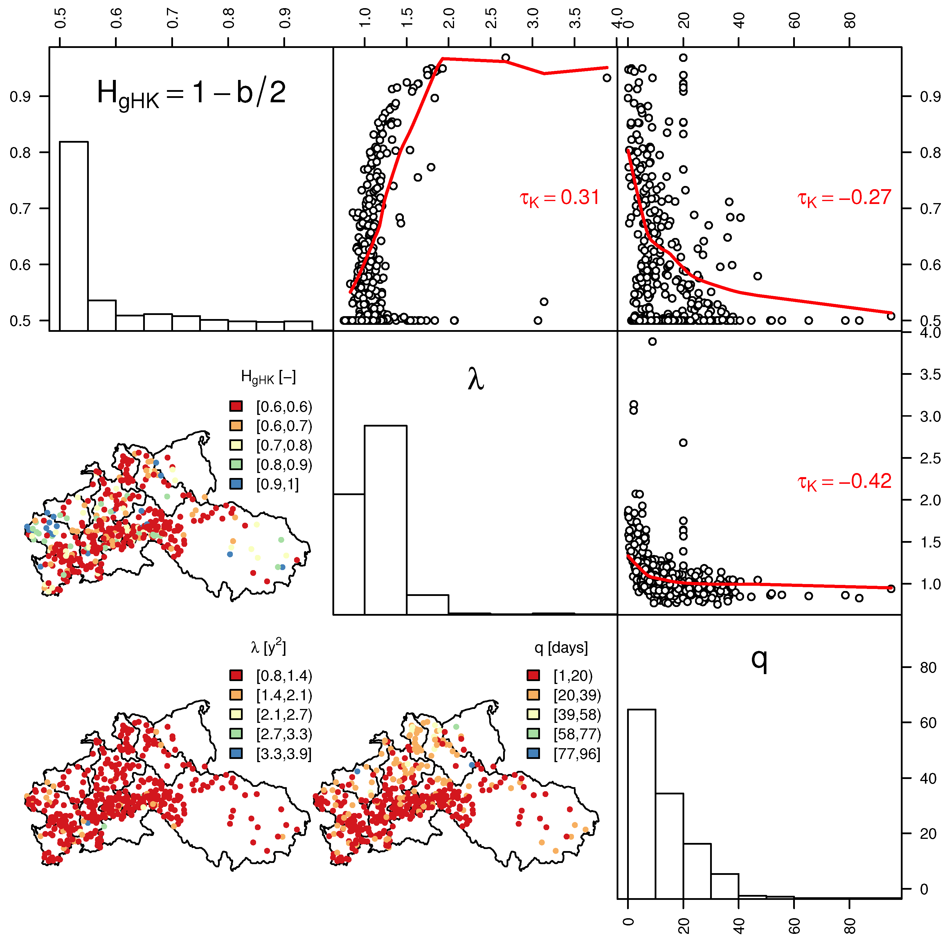
Figure 10.
Survival functions of the standardized return intervals between standardized flow values exceeding the 95% quantile threshold. The axis scales highligth the linear patterns of the exponential and Weibull distributions making the comparison with the empirical functions easier. In all panels but (b), black circles indicate the survival functions corresponding to the observed series. In panel (b) black circles indicate the survival functions corresponding to the observed shuffled (uncorrelated) data. Grey circles denote survival functions resulting from simulation by Weibull distribution (a); standard exponential distribution (b); ARFIMA (c); gHK (d); and IAAFT (e). Each panel also shows theroretical standard exponential distribution (blue line) and Weibull distribution (red line) with shape parameter equal to the average value of H computed by climacogram.
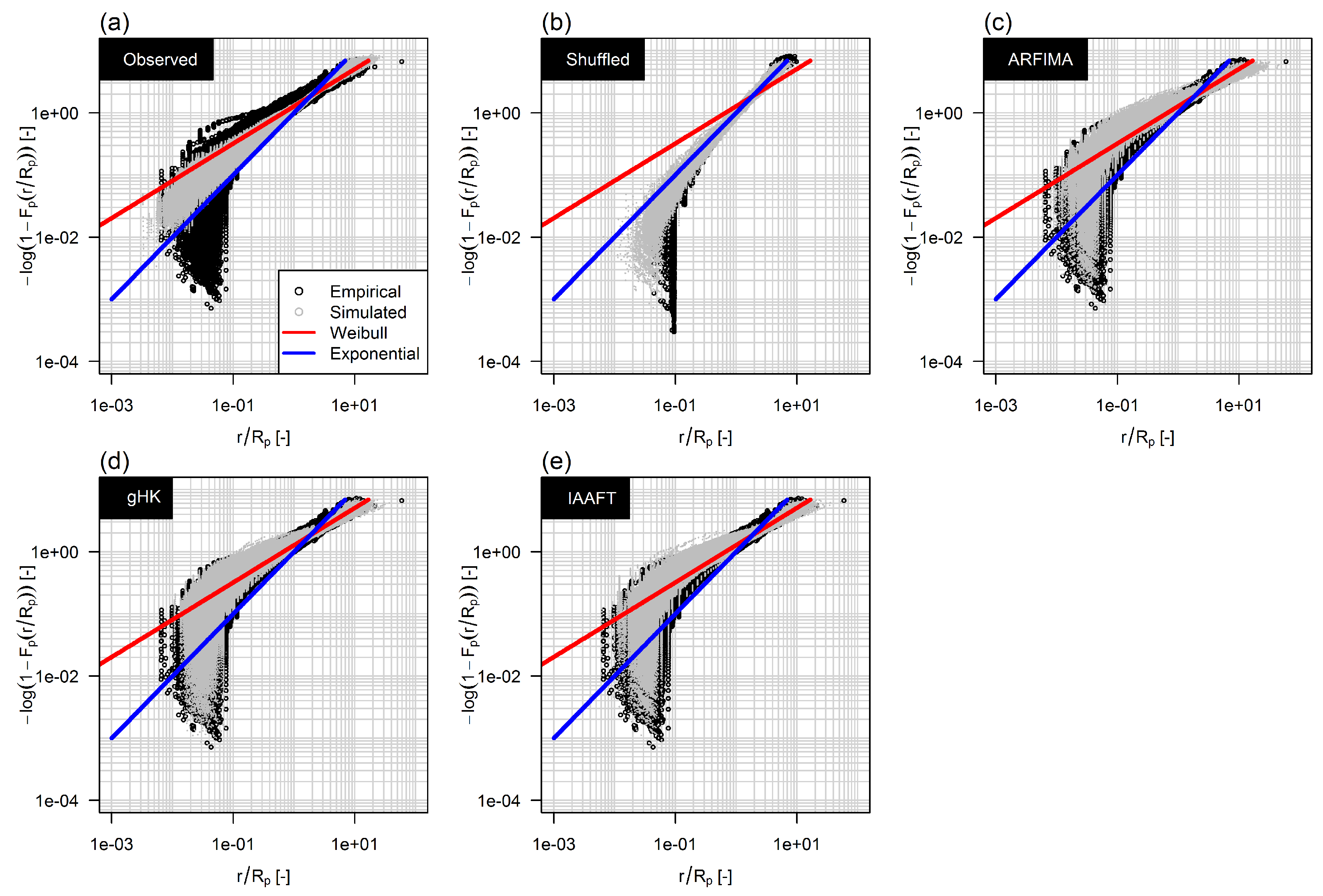
Figure 11.
(a–e) Standardized conditional return periods versus conditioning values of return intervals; (f) Box plot of standardized conditional return periods and conditioned on the values of return intervals below (−) and above (+) the median; Results in panel (f) correspond to those in panels (a–e) but for only two classes of conditioning values.
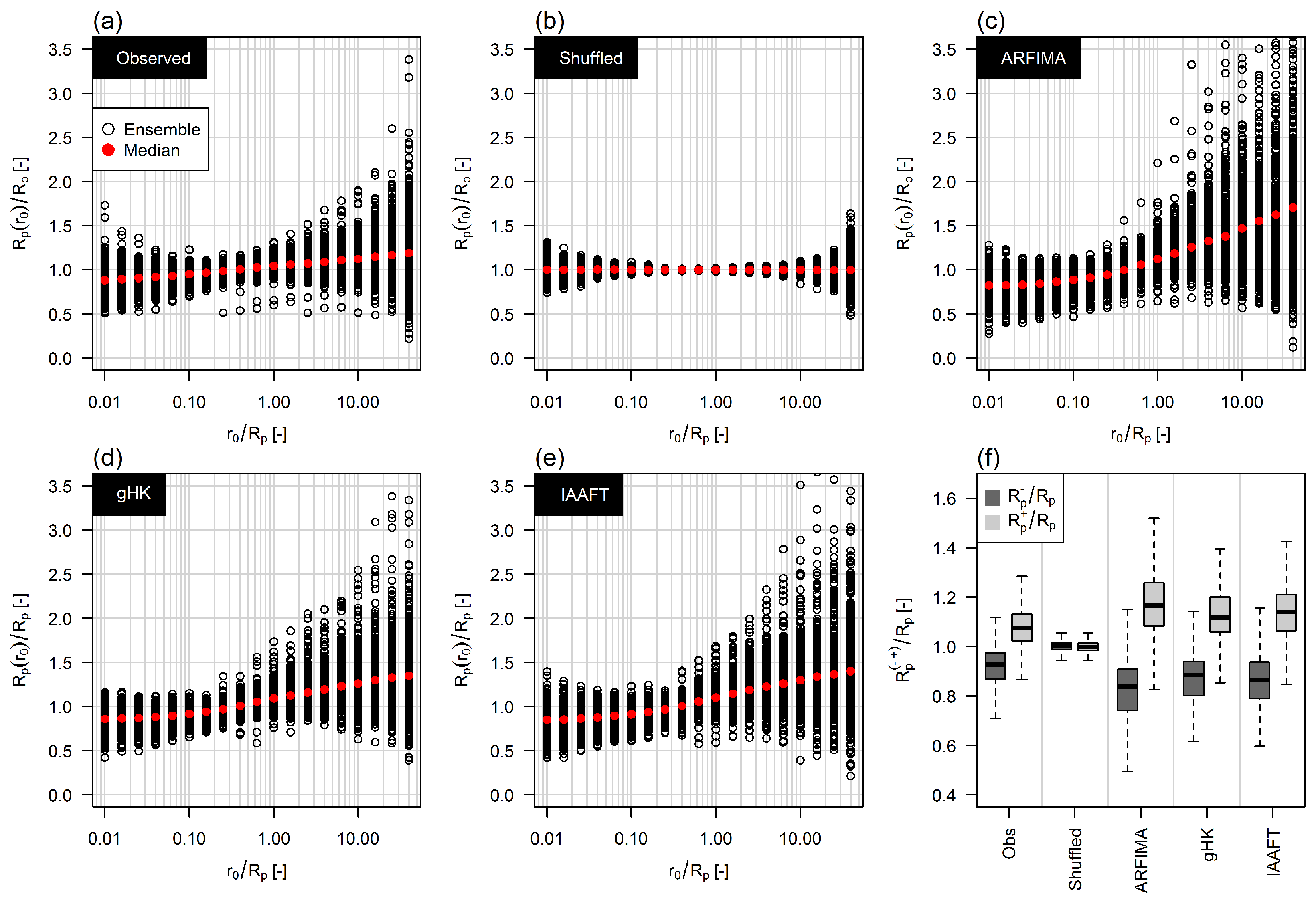
Figure 12.
Hazard functions based on the standardized return intervals between standardized flow values exceeding the 95% quantile threshold. Similar to Figure 10, in all panels but (b), black circles indicate the hazard functions corresponding to the observed series. In panel (b) black circles indicate the hazard functions corresponding to the observed shuffled (uncorrelated) data. Grey circles denote hazard functions resulting from simulation by Weibull distribution (a); standard exponential distribution (b); ARFIMA (c); gHK (d); and IAAFT (e). Each panel also shows theroretical standard exponential hazard functions (blue line) and Weibull hazard functions (red line) with shape parameter equal to the average value of H computed by climacogram.
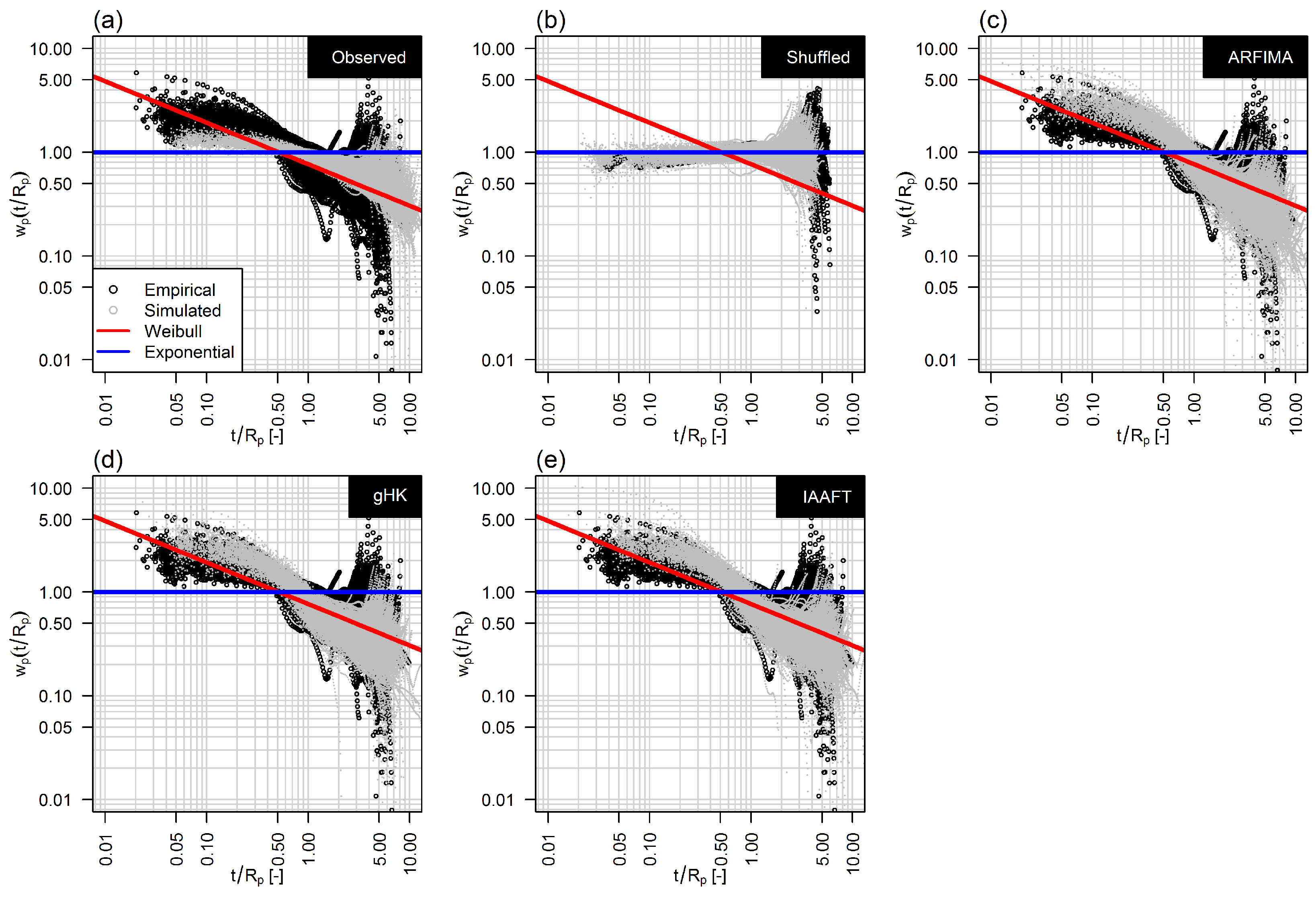
Figure 13.
Survival functions of the standardized return intervals between standardized flow values exceeding the 95% quantile threshold. Black circles correspond to the observed series while grey circles indicate an ensemble of 100 simulated time series with the same length of the observed ones. Panels (a–c) refer to the Braye River while panels (d–f) to the Escotais River. The same interpretation of Figure 10 applies.

Figure 14.
Standardized conditional return periods versus conditioning values of return intervals. Blue points correspond to the observed series, grey circles denote to an ensemble of 100 simulated time series with the same length of the observed ones, and red points denote the simulated median patterns. Panels (a–c) refer to the Braye River while panels (d–f) to the Escotais River. The same interpretation of Figure 11 applies.

Figure 15.
Box plots of the Kendall correlation coefficient between and N for observed and simulated data referring to flow values exceeding the three quantile thresholds. Shaded area denotes the 95% confidence interval around the zero value for the average sample size of the pairs .
Figure 15.
Box plots of the Kendall correlation coefficient between and N for observed and simulated data referring to flow values exceeding the three quantile thresholds. Shaded area denotes the 95% confidence interval around the zero value for the average sample size of the pairs .

Figure 16.
Illustrative ECDFs of for observed and simulated data referring to the Escotais River. Grey lines denote an ensemble of 100 curves resulting from time series simulation.
Figure 16.
Illustrative ECDFs of for observed and simulated data referring to the Escotais River. Grey lines denote an ensemble of 100 curves resulting from time series simulation.

Figure 17.
(a–f) Summary statistics of for the 473 time series included in this study, and the 95% quantile threshold.
Figure 17.
(a–f) Summary statistics of for the 473 time series included in this study, and the 95% quantile threshold.

Figure 18.
Spatial distribution of bias of summary statistics reported in Figure 17. Positive (negative) values denote model overestimation (underestimation).
Figure 18.
Spatial distribution of bias of summary statistics reported in Figure 17. Positive (negative) values denote model overestimation (underestimation).


© 2016 by the authors; licensee MDPI, Basel, Switzerland. This article is an open access article distributed under the terms and conditions of the Creative Commons by Attribution (CC-BY) license (http://creativecommons.org/licenses/by/4.0/).
Share and Cite
MDPI and ACS Style
Serinaldi, F.; Kilsby, C.G. Understanding Persistence to Avoid Underestimation of Collective Flood Risk. Water 2016, 8, 152. https://doi.org/10.3390/w8040152
AMA Style
Serinaldi F, Kilsby CG. Understanding Persistence to Avoid Underestimation of Collective Flood Risk. Water. 2016; 8(4):152. https://doi.org/10.3390/w8040152
Chicago/Turabian StyleSerinaldi, Francesco, and Chris G. Kilsby. 2016. "Understanding Persistence to Avoid Underestimation of Collective Flood Risk" Water 8, no. 4: 152. https://doi.org/10.3390/w8040152
Note that from the first issue of 2016, this journal uses article numbers instead of page numbers. See further details here.