Network Capacity Assessment and Increase in Systems with Intermittent Water Supply

Abstract

Water supply systems have been facing many challenges in recent decades due to the potential effects of climate change and rapid population growth. Water systems need to expand because of demographic growth. Therefore, evaluating and increasing system capacity is crucial. Specifically, we analyze network capacity as one of the main features of a system. When the network capacity starts to decrease, there is a risk that continuous supply will become intermittent. This paper discusses how network expansion carried out throughout the network life span typically reduces network capacity, thus transforming a system originally designed to work with continuous supply into a system with intermittent supply. A method is proposed to expand the network capacity in an environment of economic scarcity through a greedy algorithm that enables the definition of a schedule for pipe modification stages, and thus efficiently expands the network capacity. This method is, at the same time, an important step in the process of changing a water system from intermittent back to continuous supply—an achievement that remains one of the main challenges related to water and health in developing countries.

1. Introduction

The world population is increasing at an exponential rate and available water resources are reducing due to pollution and the effects of the climate change that increase the severity of droughts and favor other extreme events [1]. This places stress on many public services and dramatically increases the gap between water supply and demand. In many countries, urban growth has exceeded, and continues exceeding, the growth of supply infrastructure [2]. This growth generates the conditions necessary for operators of water supply systems to embrace intermittent water supply (IWS) [3]. Many countries in Africa, Asia, and Latin America have IWS [4].

Reducing poverty and improving public health is an important part of the Millennium Development Goals [5]. Achieving this goal is threatened by water shortages, lack of supply guarantees [6] and poor quality of supplied water. Although it is considered that the drinking water supplied through pipeline systems is safe, many studies show that deficiencies in the network, caused by IWS, can create conditions so that water is not safe and reliable [7,8,9,10,11,12,13]. The lack of reliable water supply systems in developing countries can undermine much of the hope for improvements in public health [14], and have negative effects for drinking water system objectives [15].

IWS generally seeks to reduce the per capita water demand based on savings in capital and operating costs. However, instead of being smart, this strategy brings negative consequences that outweigh the positive factors [16,17]. Symptoms of system failure include very low levels of pressure, and insufficient supply in the remotest and highest points. Generally, intermittent supply is adopted by necessity rather than by design and results in serious system impairment [18].

The best way to protect water quality is by maintaining positive and continuous pressures throughout the network [13,19]. Thus, continuous water supply ensures security. The supply change from intermittent to continuous is one of the main challenges concerning water and health in developing countries [20].

The cost of risks to the health of users must also be considered (in terms of their incomes, medical treatments, etc.) as it is much greater than the cost of replacing deficient pipes [11] that are detrimental to continuous water supply.

According to several studies [21,22,23], IWS systems produce insufficient pressure in less favored sectors or areas (nodes located on high points and/or far away). Such conditions may be favorable for reducing water losses. However, they also produce inequity in the supply [18].

Insufficient funding and mismanagement [17] are two of the main causes of the origin of IWS. System improvements in these scenarios do not derive from increasing the water supply sources, but from improving system infrastructure and management. However, a shortage of funding does not allow operators to make large investments, so they should look for profitable long term planning strategies. In this sense, phased or gradual improvements can be a good option.

The growth of cities occurs horizontally and/or vertically, as a result of residential, industrial, and commercial developments, and community facilities, etc. [24]. This growth requires expanding the network capacity and the correction of anomalies or reduced system performance [25].

When undertaking the expansion of a water supply network, the goal is to supply a much larger demand. However, when this expansion does not take into account the network capacity and the influence of the new expansion, various scenarios may appear that reduce the capacity of the network and threaten the quantity and quality of the service. Reducing the capacity of the network may lead, for example, to intermittent supply.

Generally, the network of an IWS system has insufficient capacity. However, this situation can be imperceptible because the operators manage to cover the demanded flows through differentiation of supply schedules, sectorization, and use of household tanks. Increasing the network capacity in IWS systems that seek to reach continuous water supply (CWS) is a task that must be carefully analyzed.

In this paper, the theoretical maximum flow is proposed as an indicator of network capacity. This element is endowed with its true dimension as a quantitative element that is crucial in decision-making, assessment, management, maintenance, exploitation, and design of drinking water distribution systems.

The theoretical maximum flow is important to evaluate the behavior and evolution of a drinking water system and its relationship with intermittent supply. It also serves as a basis for proposing a greedy algorithm that enables the definition of a schedule for pipe modification stages, and thus efficiently expands network capacity.

The case of study has two parts. In the first part, we evaluate the growth of the southern subsystem of the city of Oruro (Bolivia), which was originally built to offer continuous supply. However, various network modifications imposed an ideal environment for intermittent supply. In the second part, we consider the possibility of increasing the current network capacity, as part of various actions to revert to CWS. Based on the IWS classification given by Totsuka et al. [17], the system only suffers economic scarcity and management problems, and not physical scarcity. Thus, only the actions related to infrastructure improvement are analyzed.

2. Methodology

This paper discusses how poorly planned network expansions can lead from CWS to IWS. We propose the use of the theoretical maximum flow as an indicator for evaluating the network capacity, and then analyzing its relationship with intermittent supply.

Generally, the capacity of a water distribution network is considered a qualitative concept, which is usually identified from user complaints of pressure reduction [26].

We consider that network capacity represents the maximum demand (or flow) that can be met while maintaining suitable pressures throughout the network, and strictly ensuring the minimum pressure required at the node with the lowest pressure. When this flow does not cover the demand of the population, the network has insufficient capacity. Given this scenario, the network responds by reducing pressure at nodes to achieve total user demand. This situation may threaten the continuity of water supply. Even though it is possible to use a PDD (pressure driven demand) analysis, in low pressure networks, a more conservative and, thus, safer design is obtained by making use of mathematical models using demand driven analysis (DDA), and representing its capacity deficiency as a flow magnitude, since negative pressures have no physical meaning in cases of deficient network capacity.

We propose the use of the theoretical maximum flow calculated with the pressure-restricted setting curve, explained later. To evaluate the capacity of a system network with IWS, the maximum theoretical flow is compared with the maximum flow required by the population in continuous supply. It is thus possible to establish the potential of converting CWS into IWS. Intermittent water supply is usually caused by the extension of the distribution network beyond its hydraulic capacity [27].

Therefore, a method is also proposed to increase the capacity of the network, as a part of a project for gradual transition towards CWS, while taking into account that the system suffers insufficient funding.

It is common to gradually carry out the process of expanding the network capacity with more or less localized interventions on its components, so as not to endanger the service and ensure a greater lifespan for the infrastructure [25].

Another important restriction on some systems with IWS is related to the economic constraints of the water company. Therefore, we propose a gradual expansion of capacity divided into stages, in which a schedule is defined for every stage (the optimal option being sought in each of these stages). Taking advantage of improvements in network capacity, CWS gradually spreads until the entire network is covered.

When a network requires expansion, it is common practice to use optimization techniques to find a solution with lower costs and satisfactory pressures. However, these processes tend to define the overall set of pipes regardless the necessary actions associated with stage-divided projects.

In this paper, the use of the theoretical maximum flow reduces the search space to an area equal to the number of pipes evaluated and multiplied by the number of candidate diameters and number of stages.

This advantage enables us to propose the strategic replacement of pipes in a context of economic scarcity by a greedy algorithm that enables the optimal option in each of the stages to be selected—in an attempt to reach an optimal general solution. A schedule of the stages for modifying the network is defined in this way, and the result is a gradual and more efficient transition to CWS.

As the influence of each of the pipes in the total capacity of the network is known, another advantage of the proposed method is the possibility of detecting bottlenecks in the network.

2.1. System Setting Curve

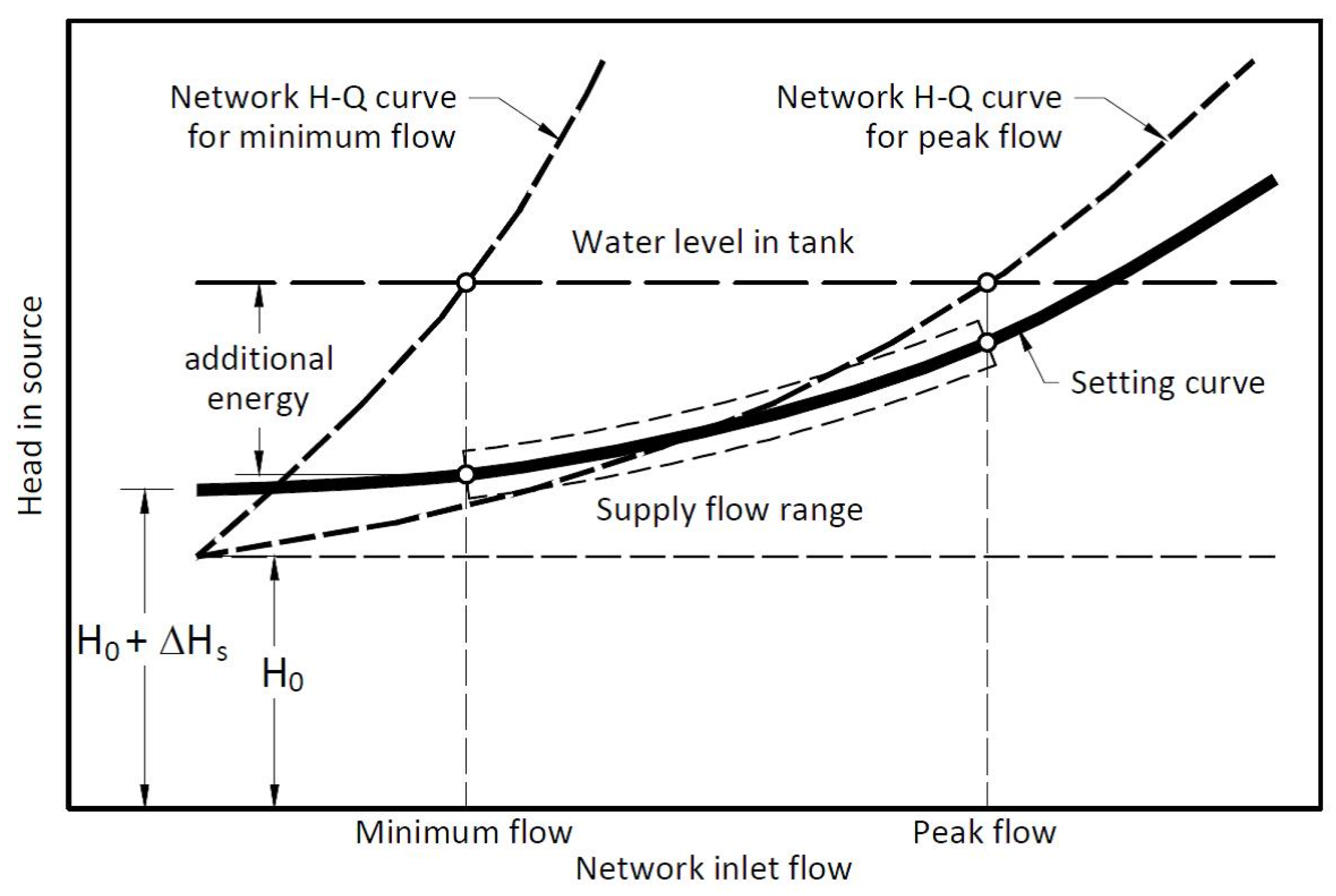
The setting curve is a very useful tool in the operation and management of a water supply system. This curve represents the need for energy production at the source in relation to the injected flow in the system, guaranteeing the minimum pressure at less favorable points. A distribution network does not have a well-defined resistance curve [28,29], because the curve slope changes—depending on the flow requirements and the resistance imposed on the network by user demand [30], from demand for minimum flows to demand for peak flows. However, the setting curve maintains a stable position, which is very advantageous and useful for solving problems related to water supply (see Figure 1).

For the calculation of the setting curve, a reliable mathematical model of the network should be available. Thus, it is possible to evaluate the losses in terms of various load conditions in the network. Tracking the setting curve at all times ensures that the pressure injected into the households is that which is strictly necessary to provide a good service. This produces energy savings. Similarly, adhering to the curve moderates pressure fluctuations in the network, thus reducing the negative implications of such variations in the life span of the network [29].

The setting curve is used for control purposes in pumping systems [29] and in energy optimization of water supply systems [31,32,33]. An approximation to the setting curve is also used as a flow modulation curve or as a setting curve for pressure reducing valves in response to changes in system demands to optimize the operation of a district metered area [34,35].

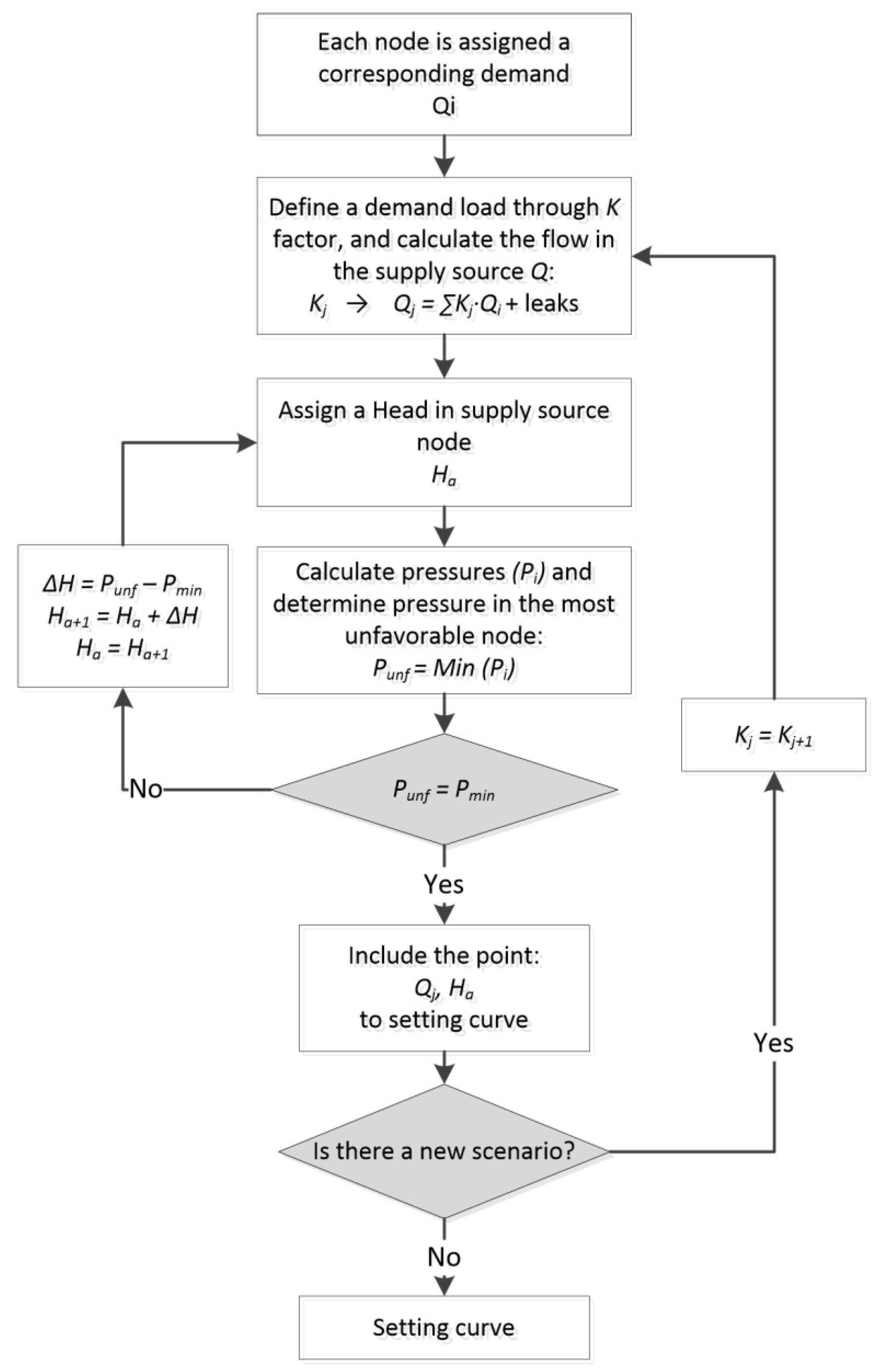
The flowchart in Figure 2 summarizes the steps to determine the setting curve when there is only one feed point. In addition to the mathematical model of the network, the minimum pressure at the nodes (P_min) must also be given. This value will define the level of service to be achieved. Subsequently, scenarios for different load states, j, defined by peak factor K applied to the demand of all the nodes must be generated. Each load condition establishes an injected flow (Q_j) in the network that requires an available head at the source (H_a) that ensures the minimum pressure in less favorable nodes (P_unf). These pressures are compared with the minimum pressure until a desired very small margin of error is reached. The set of points thus obtained describes the setting curve. The hydraulic calculation for each load state is performed with DDA. It is recommended that, like in pressures, elevation and head units be meters; and the flow in liters per second.

2.2. Theoretical Maximum Flow

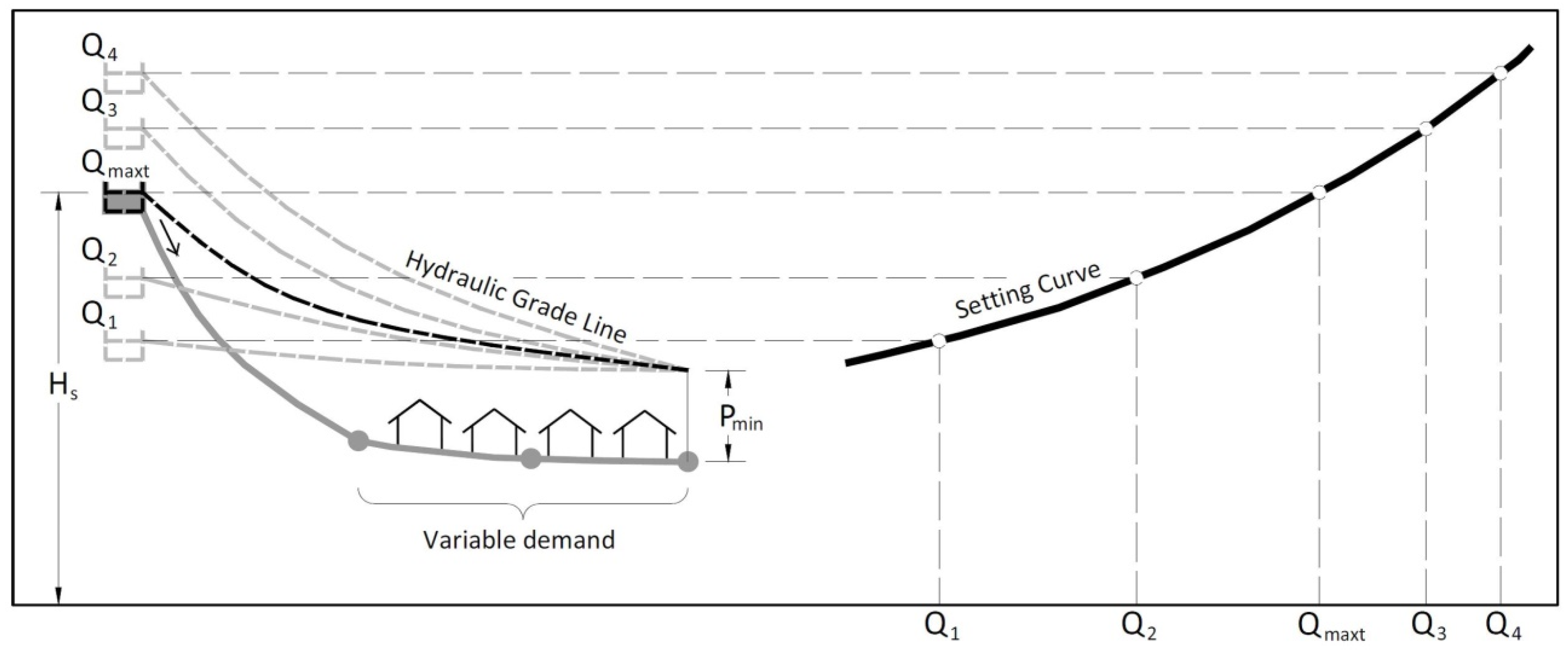
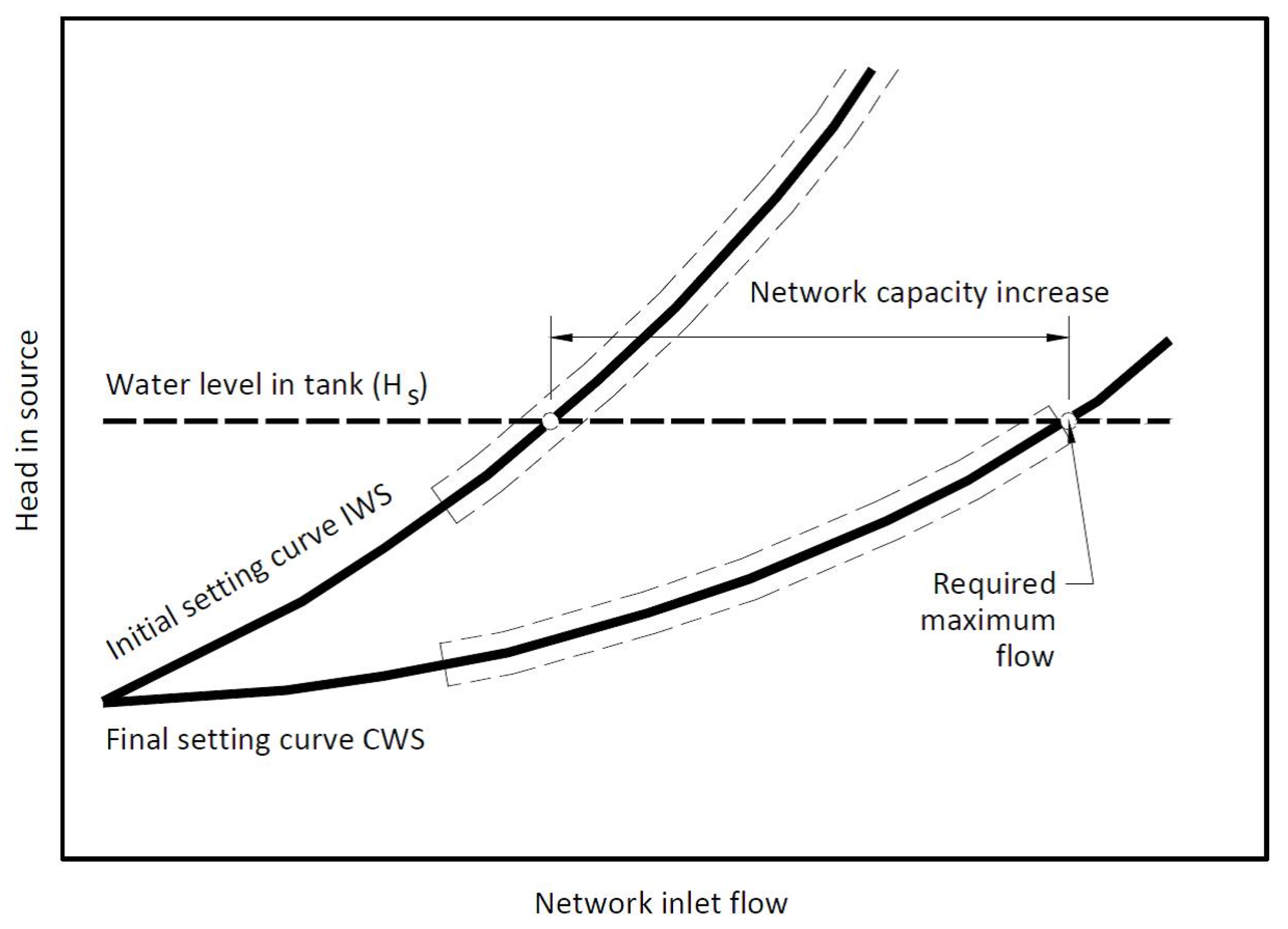
We consider the theoretical maximum flow, as the maximum flow value that can be injected in the network by ensuring that the pressure is not lower than a minimum value established as a constraint. This flow represents the theoretical capacity of the distribution network.

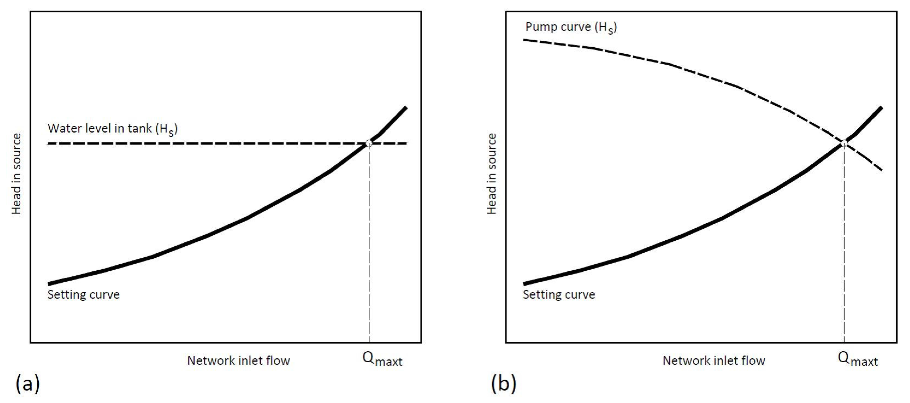
The maximum flow through a simple pipe can be calculated by taking into account the upstream and downstream boundary conditions in terms of gauge pressure or head. In a network the calculation may be similarly performed. The downstream boundary conditions are set by the setting curve, which was built to meet a defined minimum pressure (P_min). The upstream condition, which provides the hydraulic potential of the network, is defined by the hydraulic head available at the source (H_s), which can be a reservoir (Figure 3) or a pump. The theoretical maximum flow (Q_maxt) is determined by the intersection of the setting curve and the supply curve (see Figure 4).

The theoretical maximum flow or network capacity can be increased by changes in the supply source: by, for example, building new reservoirs or increasing the pump power or the number of pumps; reducing minimum pressure; and modifying the network (adding reinforcement, greater interconnectivity, making replacements, etc.). In our study, we address the latter case.

The theoretical maximum flow is strongly related to the setting curve which varies according to the network configuration, and the changes in the pipes or the service minimum pressure. One way to increase the network capacity without altering H_s is by changing the slope of the setting curve. This can be achieved by changing some physical characteristics of the network pipes.

2.3. Required Maximum Flow

For the process of increasing the capacity of the network it is necessary to have a point of reference, a target point defined by the required maximum flow (Q_maxr) and its corresponding source pressure head. In CWS, the required maximum flow corresponds to the maximum hourly flow.

The required maximum flow is calculated from the demand, using population growth forecasts, losses, and other future uses and water needs.

2.4. Procedure for Increasing the Capacity of the Network

The process of increasing the capacity of the network is very useful for the transformation of IWS into CWS. The process is based on changing the characteristics of the network so as to reduce the slope of the setting curve until the value of the required maximum flow is exceeded, see Figure 5.

Because intermittent supply systems have hydraulic, structural [3,19,20], and water quality problems [21,22,23,24,25], we consider that, in the transition process to continuous supply, replacement is more effective than pipe reinforcement.

Starting with the current network, each pipe is replaced with another pipe with a different diameter. This change is evaluated by calculating the theoretical maximum flow. Thus, it is possible to calculate the increase in capacity involved in each of the changes. By incorporating the cost of replacing a pipe p an expansion rate is determined:

$$q_{p,d}=\frac{Q_{\max t}^{p,d}-Q_{\max t}^o}{C\left(d_p\right)·L_p},$$

(1)

where q_p,d is expansion rate produced by substituting pipe p for a new pipe with diameter d; $Q_{\max t}^o \text{is}$theoretical maximum flow of the original network or the network modified in the previous step; $Q_{\max t}^{p,d}$is theoretical maximum flow after substituting pipe p for a new pipe with diameter d; C(d_p) is unit length cost of pipe p replaced with a new pipe of diameter d; and L_p is length of modified pipe p.

The expansion rate (Equation (1)) is very useful in identifying pipes that constrain the network capacity.

Another approach for selecting the pipes to be replaced, which prioritizes the flow increase over the cost, is by raising the difference in the numerator of the expansion rate (Equation (1)) to an exponent, n, as in Equation (2). In this way, the pipes will initially be modified to larger diameters. This will subsequently offset the initial cost as smaller diameters will be required.

$$q_{p,d}^n=\frac{{\left(Q_{\max t}^{p,d}-Q_{\max t}^o\right)}^n}{C\left(d_p\right)·L_p},$$

(2)

By using the expansion rate in each of the expansion stages, the pipe to be modified or replaced is identified (as the pipe with the largest expansion rate value).

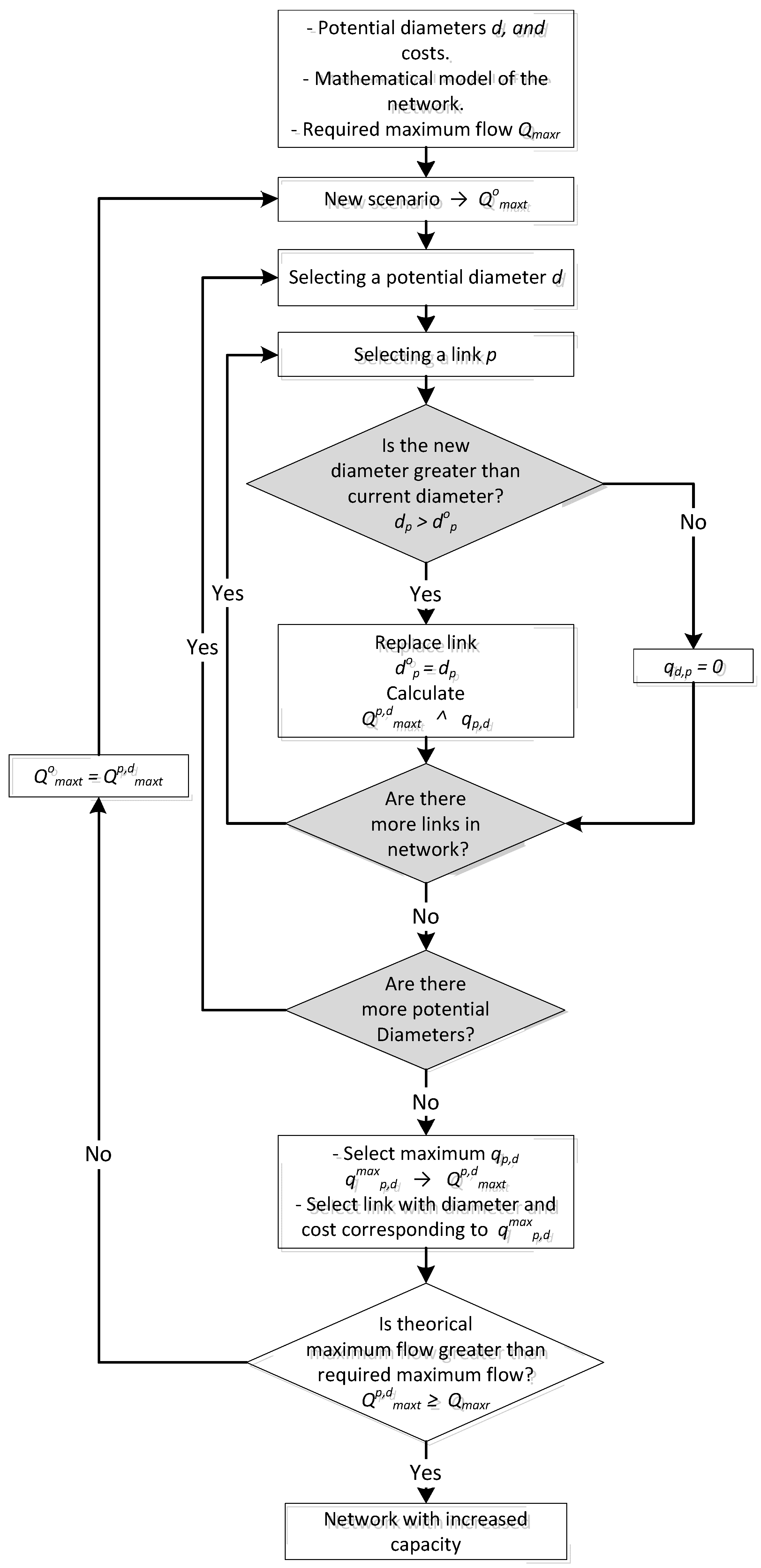
The process outlined in the flowchart in Figure 6 enables us to define a new network configuration by increasing its capacity after replacing the pipes that represent the lowest costs. The order of priority for the replacement of the pipes is also identified, and this enables us to plan the process of gradually increasing the network capacity. The total cost may be divided into stages based on this prioritization.

3. Results and Discussion

The case of study has two parts:

The first step is to reconstruct the hydraulic conditions of the subsystem in the south of Oruro in the period 1968–2013. Considering that the initial network is the main part of the current network and that it has been maintained since the inauguration of the infrastructure, we will use the current network model. Due to a lack of information, the growth of the urban area is used as a reference to reconstruct the network evolution. As a result, the topology of the network during each of the study periods is estimated. Considering the population and water demand of each of the periods studied, it is possible to calculate the required maximum flow. However, to compare this value with the network capacity it is necessary that both elements have the same dimensions. For this purpose, we propose the use of the theoretical maximum flow indicator.

In the second part, based on the current network of the south Oruro area, we seek to identify and prioritize the order of the pipes that require replacement under economic and hydraulic criteria, in order to gradually increase the network capacity to achieve the necessary infrastructure to transform IWS into CWS (24/7). Besides the theoretical maximum flow, an expansion rate indicator will also be used.

3.1. First Part of the Study

The project “Drinking water for the city of Oruro” [36] was begun in 1968 and included the main infrastructure for water supply in the southern sub-area of the city—a tank and the mains. The subsystem offered continuous supply but is currently an IWS system. There are no records of when the system became intermittent. Based on the theoretical maximum flow, the transition process is analyzed in this part of the study.

Considering the size of the urban area [37], population growth [38], population density, and the number of current users, it is possible to estimate the population growth of the study area, defined by the urban growth (

Table 1. Population and required maximum flow for the Oruro southern subsystem.

Year	Population	Qmaxr (L/s)
1968	13842	33.77
1972	16814	41.02
1985	33407	81.51
2007	37395	91.24
2013	37700	91.98

) during the given periods. Based on the current average supply of the subsystem (84.32 L/capita/d) and a peak factor of 2.5 (representative of other areas of the city that have CWS and similar population growth) the required maximum flow for each year can be calculated.

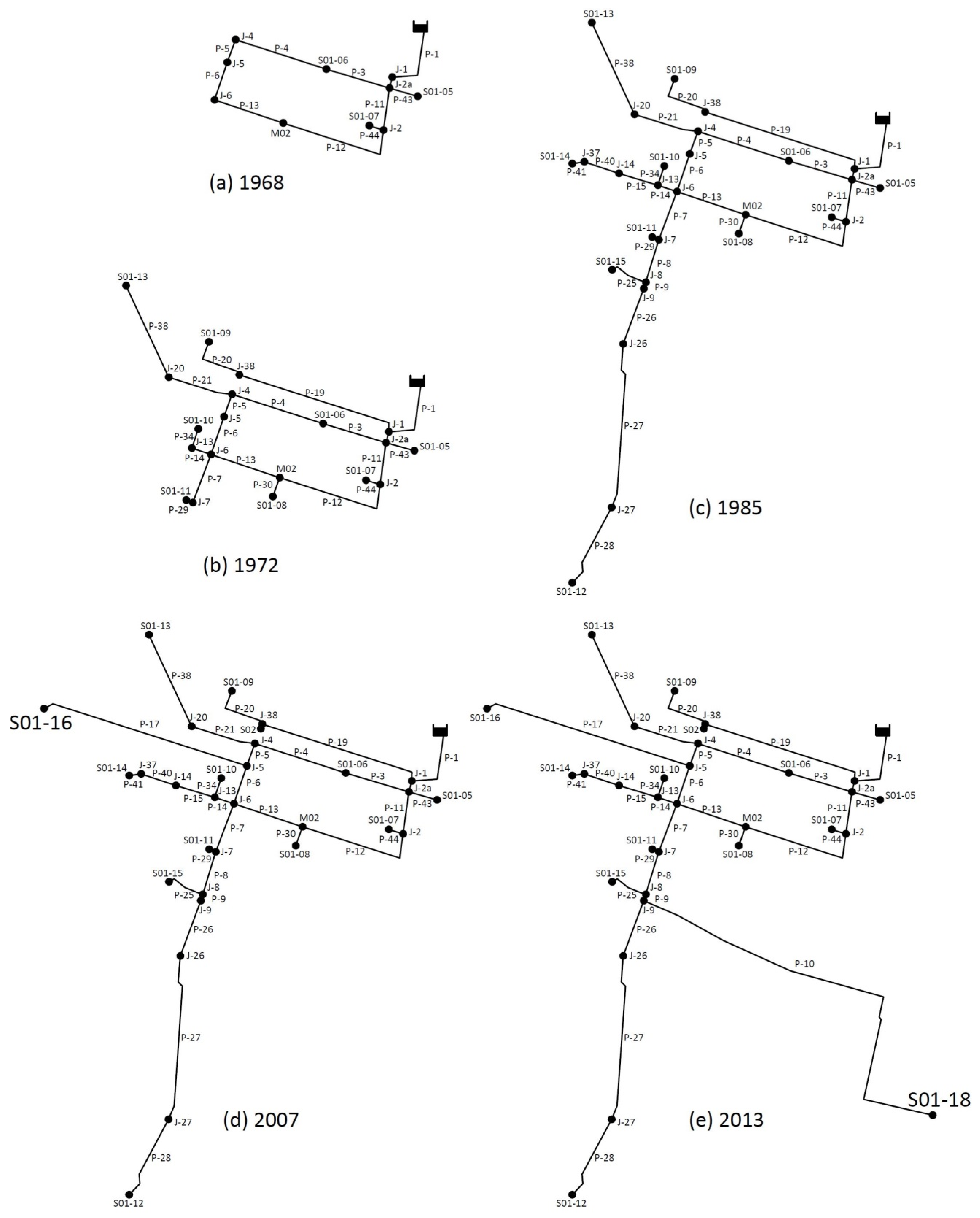
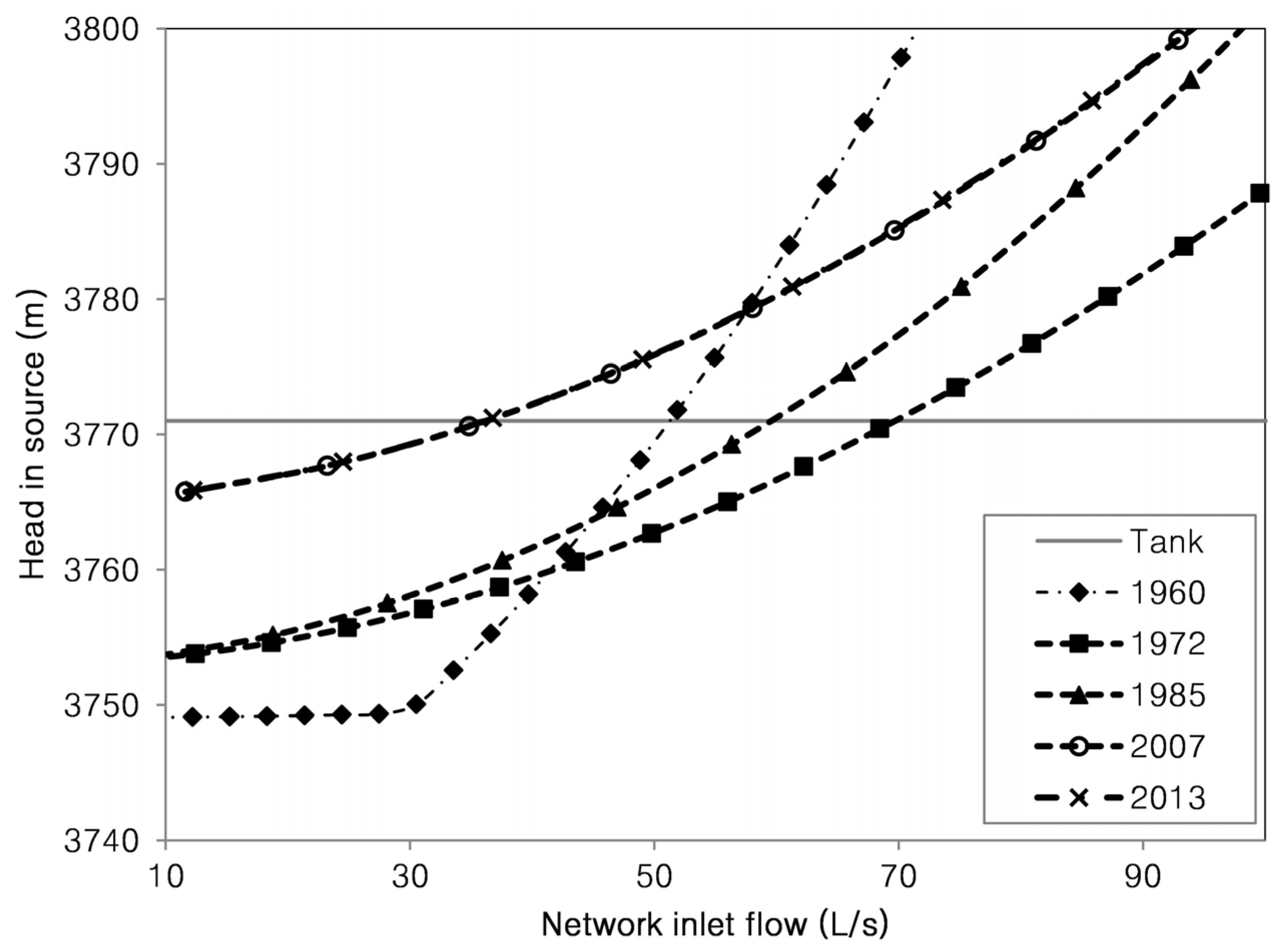
The urban growth of the city enables us to set growth scenarios for the subsystem supply network, for the changes in the mains and for the inlet to the sectors (see Figure 7). Based on these scenarios, the setting curve and the theoretical maximum flow or capacity of the network (Figure 8) is calculated. A minimum pressure (P_min) condition of 20 m is adopted; the minimum elevation of the water level in the reservoir (H_s) is 3771 masl (meters above sea level), and the average elevation of the network is 3723.8 masl.

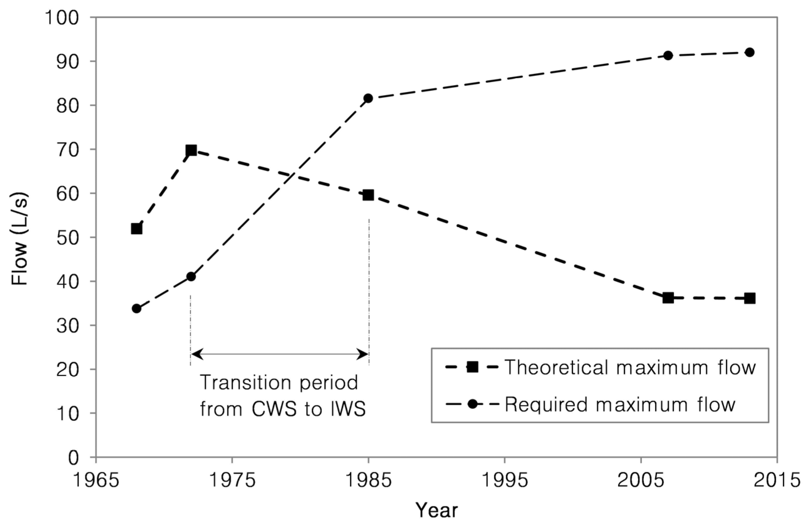
Comparison between the required maximum flow and the theoretical maximum flow or network capacity is shown in Figure 9.

The studied system was designed for continuous supply. This is evident because in 1968 the network capacity was greater than the required maximum flow. The network was designed to supply water to a larger population and had a reasonable slack for expansion. This scenario was maintained throughout the first period, 1968–1972; and expansions made during this period were developed in favorable areas. These expansions were developed properly and did not significantly weaken the network capacity.

In the period 1972–1985, the situation changed. The southern region of Oruro grew faster than the rest of the city [37]. The network expansions to cover the new sectors were very large. In addition, the selection of small diameters increased the pressure drop and network capacity was therefore reduced.

In 1985, the required maximum flow exceeded the theoretical maximum flow. This fact imposed a reduction of pressure in the network. The nodes located in unfavorable areas were prone to run out of water during peak consumption. People needed to protect their supply and opted for the use of household tanks. This scenario led to inequity in the supply: nodes located in favorable areas squandered water, due to lack of metering, while users located in unfavorable areas complained about a lack of water. Eventually, a perception of water scarcity prevailed among the population and the operator. A solution was sought.

To solve the water shortage in less favorable points, there are two potential solutions: the first option, though not very evident in scenarios of economic scarcity and poor management, is to expand the capacity of the network by replacing and reinforcing the mains; and the second option is to opt for intermittent supply (a widespread misconception derived from a lack of water and funding).

The adoption of intermittent supply limits the hours of supply in different areas, setting schedules that seek to reduce the required maximum flow. This action may be useful initially as the main sections transport lower flow rates during peak consumption and therefore sufficient flow reaches the points located in unfavorable areas. However, population growth will require expansion and this condemns the system to intermittent supply.

In this second period, the theoretical maximum flow and the required maximum flow curves intersect. A point was reached at which the capacity of the network no longer met the demand of the population with continuous supply (this situation has been maintained since then). Accordingly, we can say that a policy based on an IWS approach was implemented in the south of Oruro starting between 1970 and 1985 (see Figure 9).

In the third study period, 1985–2007, intermittent supply was consolidated. New expansion further reduced the capacity of the network. The expansion of the S01-16 sector used diameters that were too small and, in addition, supply was extended to an even higher point. These features made it a critical point, which conditioned the setting curve severely and, consequently, the value of the theoretical maximum flow.

Between 2007 and 2013, the subsystem was expanded with the S01-18 sector, which did not affect the capacity of the network because the sector is in a lower area and the installed diameters were suitable for the needs of the sector. It proved to be a good expansion, since it did not greatly affect the setting curve and the theoretical maximum flow.

The reduction of network capacity is a problem not perceived when the network works with intermittent supply, because water reaches all sectors, although at very low pressures; however, this situation will be primarily responsible for inequitable supply.

3.2. Second Part of the Study

The capacity of the subsystem network in the south of Oruro is currently insufficient and, as a result, supply is intermittent. It is necessary to increase this capacity if the aim is to achieve continuous supply. Due to a shortage of funds, the expansion is bound to be gradual and staged. Accordingly, it is necessary to know the order of pipe replacement. The budget available annually for the process of increasing the network capacity is Bs. 700,000 (seven hundred thousand Bolivian boliviano, equivalent to €89,172). The transition from IWS to CWS requires that the network has a capacity for continuous supply of 91.98 L/s.

Unit costs, which include all the elements necessary for the replacement of pipes, and which depend on the diameter, are presented in

Table 2. Unit costs for replacing pipes as a function of diameter.

Diameter (mm)	Unit Cost (Bs/m)
75	385.02
100	399.66
150	442.46
200	502.93
250	608.39
300	703.17
350	832.61
400	1,030.54
500	1,371.51

.

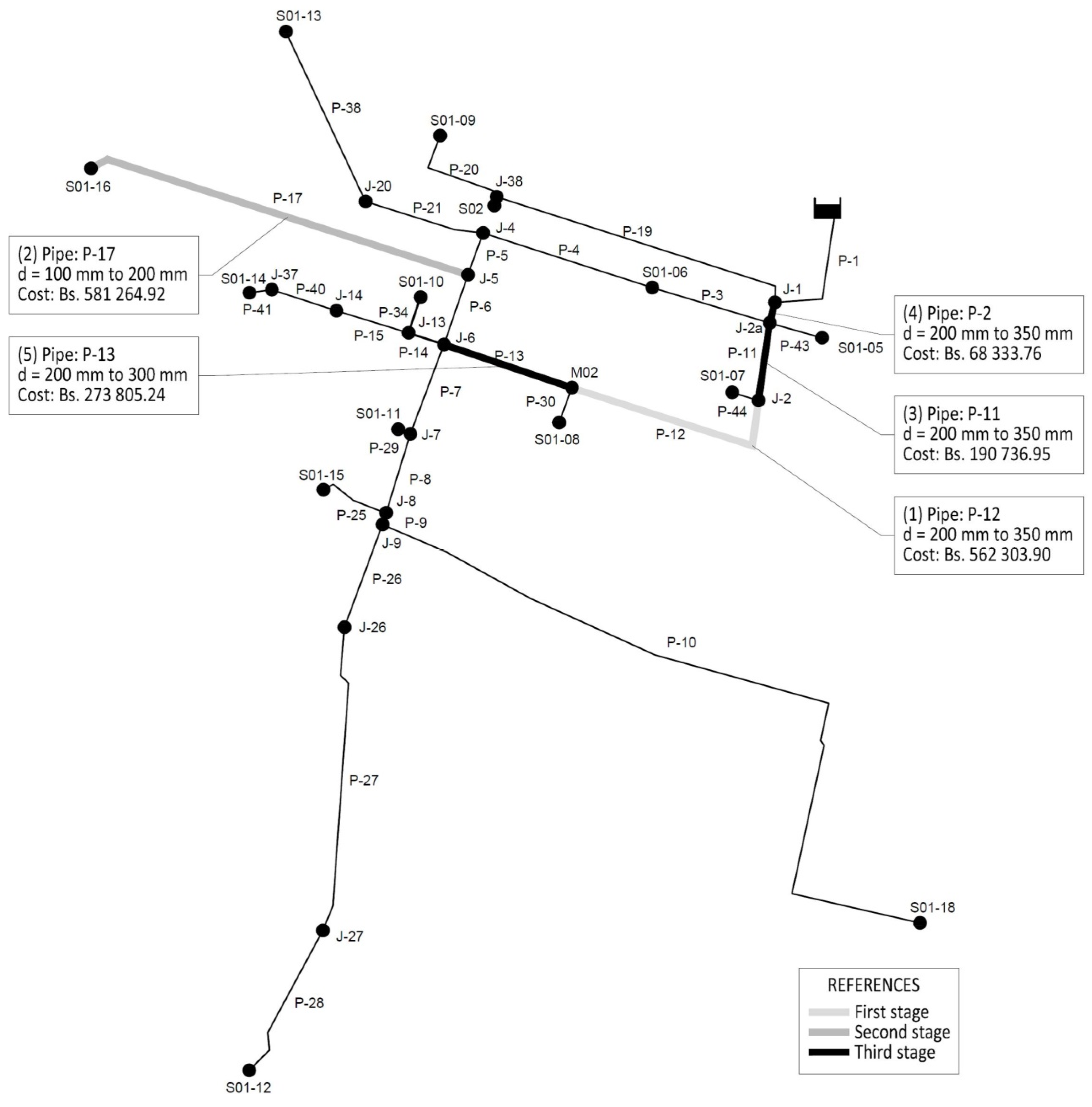
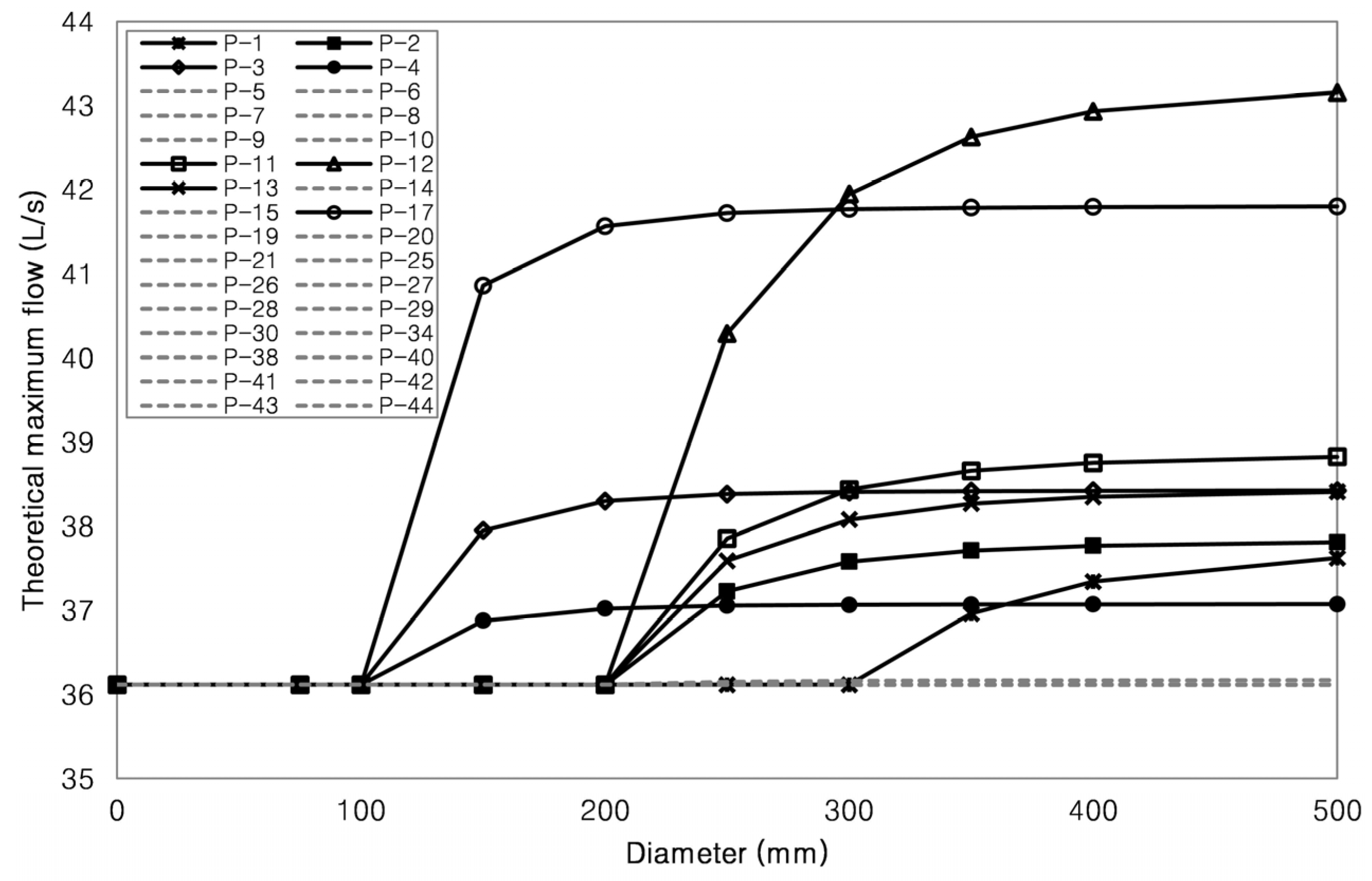
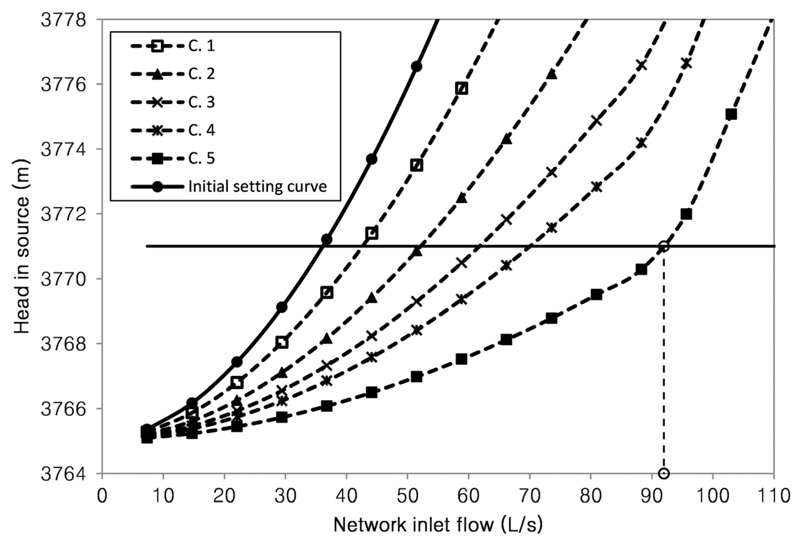
When large diameter pipes are changed, the theoretical network maximum flow is increased (see Figure 10). This increase is more pronounced in pipes P-1, P-2, P-3, P-4, P-11, and P-13, and even more so in pipes P-12 and P-17. These last mentioned pipes are the most critical for the network and represent bottlenecks; so, any action to expand the network must take them into account. Augmenting the diameter of the remaining pipes causes minimal increases in the network capacity, so their importance in increasing network capacity is minimal. Generally, the first upgrade of diameter produces a significant increase in network capacity, while subsequent diameter upgrades do not produce such a large effect. The curve tends to reflect an asymptotic behavior (Figure 10).

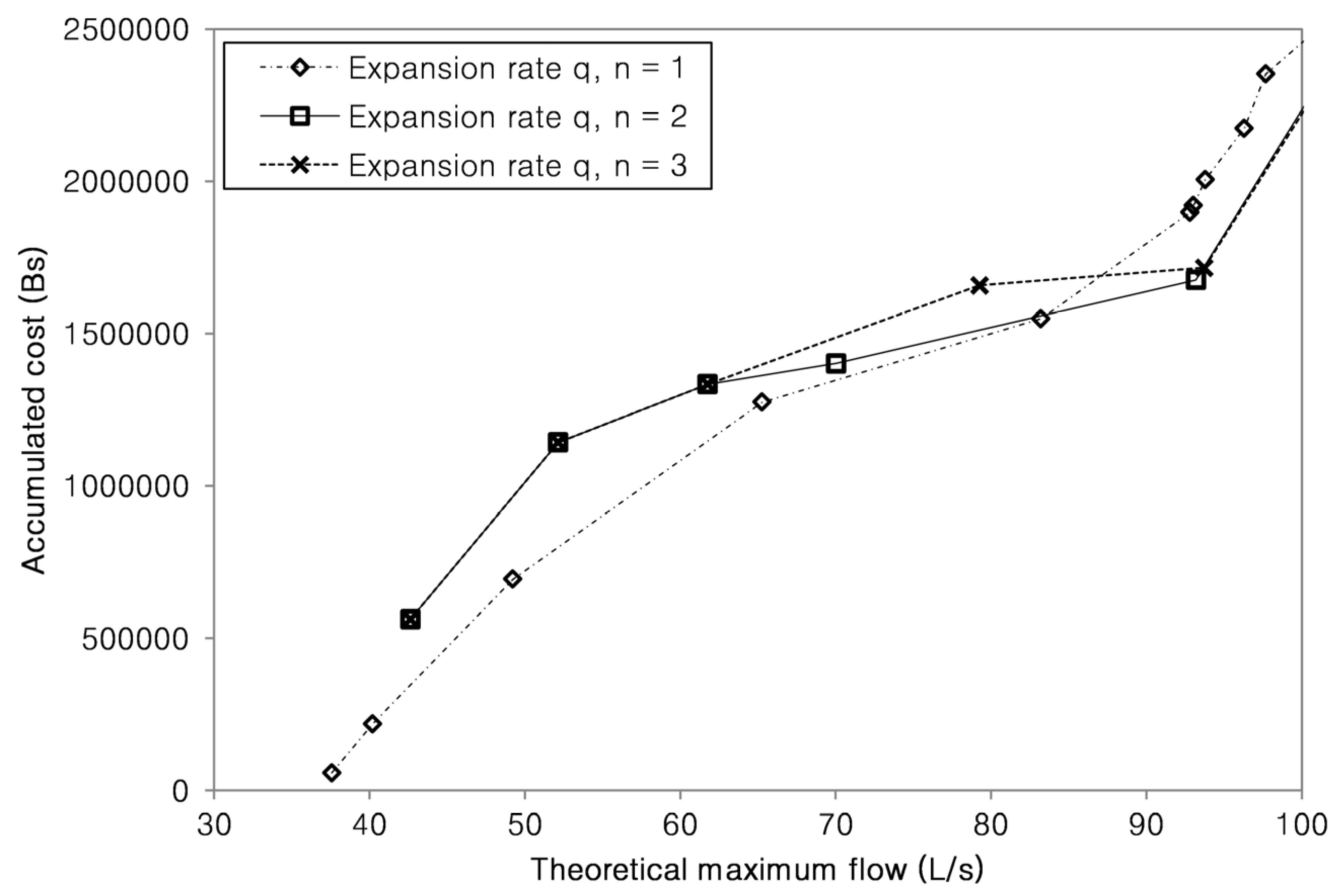
The expansion process was developed using the expansion ratio q given in Equation (2) for n = 1, 2 and 3. The exponent was chosen depending on the theoretical maximum flow (Figure 11). The use of the indicator with an exponent greater than 1 enables lower costs to be reached when the expansion flow rate is larger; however, n = 1 can be used when the maximum flow requirement is lower. In any case, it is adequate for making a comparison with indicators.

To reach the required maximum flow of 91.98 L/s, the lowest cost is produced by the indicator q with n = 2. The setting curve is gradually changed in five steps that define the order of actions for the gradual improvement (Figure 12). With this prioritization, three stages of investment (last column of

Table 3. Results of the network capacity increase process.

Iteration	qmax n = 2	Modified Pipe	New Diameter (mm)	Qmaxt (L/s)	Pipe Cost (Bs)	Accumulated Cost (Bs)	Cost per Stage (Bs)
1	0.07540	P-12	350	42.63	562,303.90	562,303.90	562,303.90
2	0.15582	P-17	200	52.14	581,264.92	1,143,568.83	581,264.92
3	0.48497	P-11	350	61.76	190,736.95	1,334,305.77	532,875.95
4	1.00235	P-2	350	70.04	68,333.76	1,402,639.54
5	1.95625	P-13	300	93.18	273,805.24	1,676,444.78

and Figure 13) are defined.

Due to increasing water-losses produced after transition from IWS to CWS [3], and which consequently increase the required maximum flow, it is necessary to implement an active leakage control [39] simultaneously with the network capacity expansion to avoid oversizing the network and wasting water.

4. Conclusions

Although its use is generally applied to CWS, the setting curve is a useful tool for evaluating and improving systems with intermittent supply.

The approach using theoretical maximum flow enables network capacity to be given its true quantitative dimension. This is necessary for decision-making in the assessment, management, maintenance, operation, and design of a continuous or intermittent supply drinking water network. Specifically, in this paper, this approach enables us to evaluate a system with intermittent supply, track its evolution from its CWS origin (first part of the study) to the current IWS, and propose solutions to recover CWS (second part of the study). Thus, this study contributes to improve intermittent supply systems, which remains one of the main challenges related to water and health in developing countries.

In the first part, we can see how poorly planned expansion processes can systematically reduce network capacity. This reduction initially brought low pressure, flow failure in unfavorable areas, and user complaints. The situation was perceived as water scarcity rather than reduced network capacity. As a result, it was decided to opt for intermittent supply. Further expansion actions consolidated this approach.

It is important to consider that the rational extension of the network not only involves laying additional pipelines that reach the point of demand, but that this process should be accompanied by the reinforcement, rehabilitation, or replacement of the network water mains.

A process of expanding network capacity, as part of the transition from IWS to CWS with poor funding, is difficult to implement. Consequently, gradually prioritizing pipe replacements, based on achieving the greatest impact on the quality of service at the lowest cost, is a very useful criterion. The characteristics of the method allow us to reach a more efficient process in small networks than in large ones.