Bivariate Drought Analysis Using Streamflow Reconstruction with Tree Ring Indices in the Sacramento Basin, California, USA

Abstract

Long-term streamflow data are vital for analysis of hydrological droughts. Using an artificial neural network (ANN) model and nine tree-ring indices, this study reconstructed the annual streamflow of the Sacramento River for the period from 1560 to 1871. Using the reconstructed streamflow data, the copula method was used for bivariate drought analysis, deriving a hydrological drought return period plot for the Sacramento River basin. Results showed strong correlation among drought characteristics, and the drought with a 20-year return period (17.2 million acre-feet (MAF) per year) in the Sacramento River basin could be considered a critical level of drought for water shortages.

1. Introduction

Generally, long-term data are recommended for analyzing floods and droughts. However, although precipitation data are available from the 16th century onwards, their quality and reliability in many countries are questionable because of the methods of observation, different periods of observations, uncertainties associated with gaging sites, and temporal resolution of observations [1,2]. Many studies have, therefore, used tree-ring data as a way to acquire data for longer periods of time, up to 500 years [3].

Since Ferguson [4] correlated observed hydro-meteorological data and tree-ring data in California, many studies have utilized tree-ring data to reconstruct time series of the past. Fritts [5] did tree ring analysis and correlated the data with climate, suggesting that it can be used in water resources management [6]. Also, some studies have correlated hydro-meteorological variables with tree-ring data to reconstruct climate factors [7,8,9,10]. Some studies have reconstructed seasonal series, such as precipitation [11,12], natural hazards [13], and temperature [14], based on tree ring width data. However, most of the studies on tree rings and hydrological phenomena have focused on droughts [15,16,17,18,19,20,21,22,23,24]. This may be because annual data are normally reconstructed using tree ring data and hence it is difficult to analyze intra-annual hydrological phenomena. Long time-scale data are mainly used for droughts, because it is difficult to determine the onset or end of a drought and often the drought may last for several months or years. The long time-scale occasionally gives rise to a sample size problem [25] for drought analysis that can be overcome with long-term tree ring reconstruction [26]. Some studies have directly correlated tree rings with droughts [15,27], drought patterns or oscillations [28,29,30], drought index and its trend [23,31,32,33], return periods [34], and spatial drought characteristics [35].

Bivariate (or multivariate) analyses of drought characteristics, such as severity, duration, and arrival time, are being increasingly made [36]. These analyses have introduced multivariate drought indices, such as Multivariate Drought Index (MDI) including precipitation, runoff, evapotranspiration, and soil moisture [37]; Multivariate Standardized Drought Index (MDSI) which combines the Standardized Precipitation Index and the Standardized Soil Moisture Index [38]; and Vegetation Drought Response Index (VegDRI) which integrates climatic indicators; and satellite-derived vegetation index [39,40]. Some studies have employed conventional multivariate analysis for drought indices with PDSI [23,41] and SWSI [42,43], or bivariate frequency analysis [44,45] assuming that all variables had the same probability distribution. To overcome this restriction, the copula method has been developed [46]. For doing bivariate drought analysis by the copula method [46,47], tree ring reconstruction can be employed to our advantage.

The objective of this study, therefore, is to reconstruct the annual streamflow of the Sacramento River in California and Oregon using tree-ring width data, and use the reconstructed data for bivariate drought frequency analysis with the copula method. Selected tree-ring data were used in an artificial neural network for streamflow reconstruction and the reconstructed data were verified by comparing with actual observations. The Archimedean copula function was applied to the reconstructed streamflow data and then the return period plot of the hydrological drought in the Sacramento River basin was derived. The advantages of using the copula method have been discussed in many studies [34,36,48,49,50,51,52,53,54,55]. Since drought may last from months to years, as has happened in California, long-term reconstruction based on tree-ring data, addresses the drawback of short-term data [56].

2. Materials and Methods

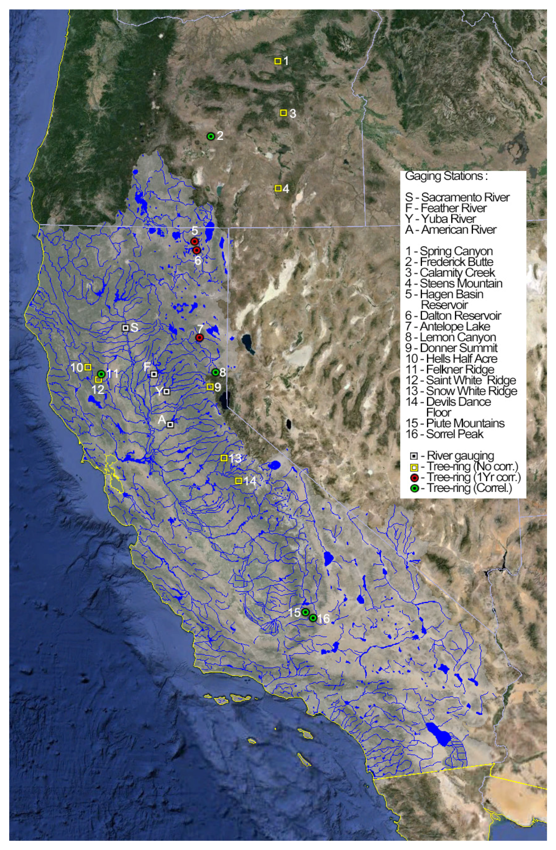
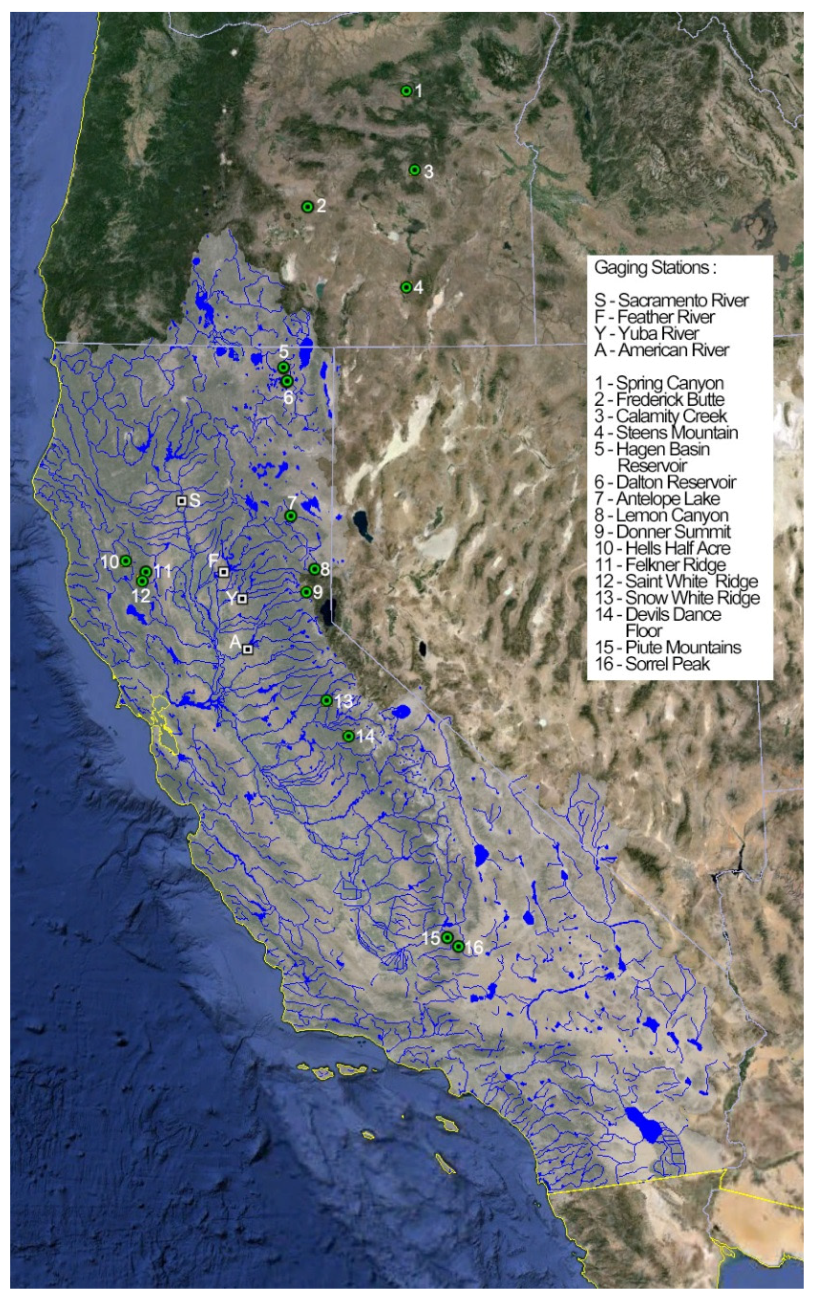
2.1. Study Area and Data

Annual streamflow data for four Sacramento rivers and tree-ring data of the nearby region were employed in this study. The tree-ring data from 17 sites (Figure 1 and

Table 1. Tree ring sites and streamflow observatory specification [58].

Category	Index in Figure 1	ID	Name	Site Location			Tree Ring Species
				Lat (degree)	Lon (degree)	Height (EL.m)
Tree ring sites	7	ANTEP	Antelope Lake	40.15	−120.6	1480	Pinus jeffreyi Balf
	7	ANTEP	Antelope Lake	40.15	−120.6	1480	Pinus ponderosa Douglas ex C. Lawson
	3	CALAM	Calamity Creek	43.98	−118.8	1464	Juniperus occidentalis Hook
	6	DALTON	Dalton Reservoir	41.62	−120.7	1531	Pinus ponderosa Douglas ex C. Lawson
	14	DEVILS	Devil’s Dance Floor	37.75	−119.75	2084	Pinus jeffreyi Balf
	9	DONNER	Donner Summit	39.32	−120.35	2265	Pinus jeffreyi Balf
	11	FELKN	Felkner Ridge	39.5	−122.67	1494	Pinus lambertiana Douglas
	2	FREDER	Frederick Butte	43.58	−120.45	1494	Juniperus occidentalis Hook
	5	HAGER	Hager Basin Reservoir	41.77	−120.75	1524	Juniperus occidentalis Hook
	10	HELLS	Hell’s Half Acre	39.6	−122.95	1922	Pinus jeffreyi Balf
	8	LEMON	Lemon Canyon	39.57	−120.25	1859	Pinus jeffreyi Balf
	15	PIUTE	Piute Mountain	35.53	−118.43	1975	Pinus jeffreyi Balf
	13	SNOWHT	Snow White Ridge	38.13	−120.05	1731	Pinus ponderosa Douglas ex C. Lawson
	16	SORREL	Sorrel Peak	35.43	−118.28	2011	Pinus jeffreyi Balf
	1	SPRING	Spring Canyon	44.9	−118.93	1366	Juniperus occidentalis Hook
	4	STEENS	Steens Mountain	42.67	−118.92	1656	Juniperus occidentalis Hook
	13	STJOHN	St. White Mountain	39.43	−122.68	1555	Pinus ponderosa Douglas ex C. Lawson
Flow site	S	SBB	Sac. River, Abv bend bridge	40.29	–122.19	56.6	-
	F	FTO	Feather River, Oroville	39.52	–121.55	45.4	-
	Y	YRS	Yuba River, Smartville	39.24	–121.27	85.3	-
	A	AMF	American River, Folsom	38.68	–121.18	0	-

) in California and Oregon, which reflect standard chronologies of ring width [57], were obtained from the International Tree-Ring Databank [58]. The tree ring width data were standardized [59]. Annual streamflow is the sum of four river flows, which are the Sacramento River above Bend Bridge (SBB), the Feather River at the Lake Oroville (FTO), the Yuba River near Smartville (YRS) and the American River at Folsom (AMF), which was obtained from the California Data Exchange Center of California Department of Water Resources [60] for the period 1872 to 1977. It has a long-term mean of 18.9 MAF (million acre-feet; 1.23 × 10⁹ m³), median of 17.6 MAF, and maximum flow of 51.6 MAF that occurred in the year 1890. These tree ring and streamflow sites are shown in Figure 1 and Table 1.

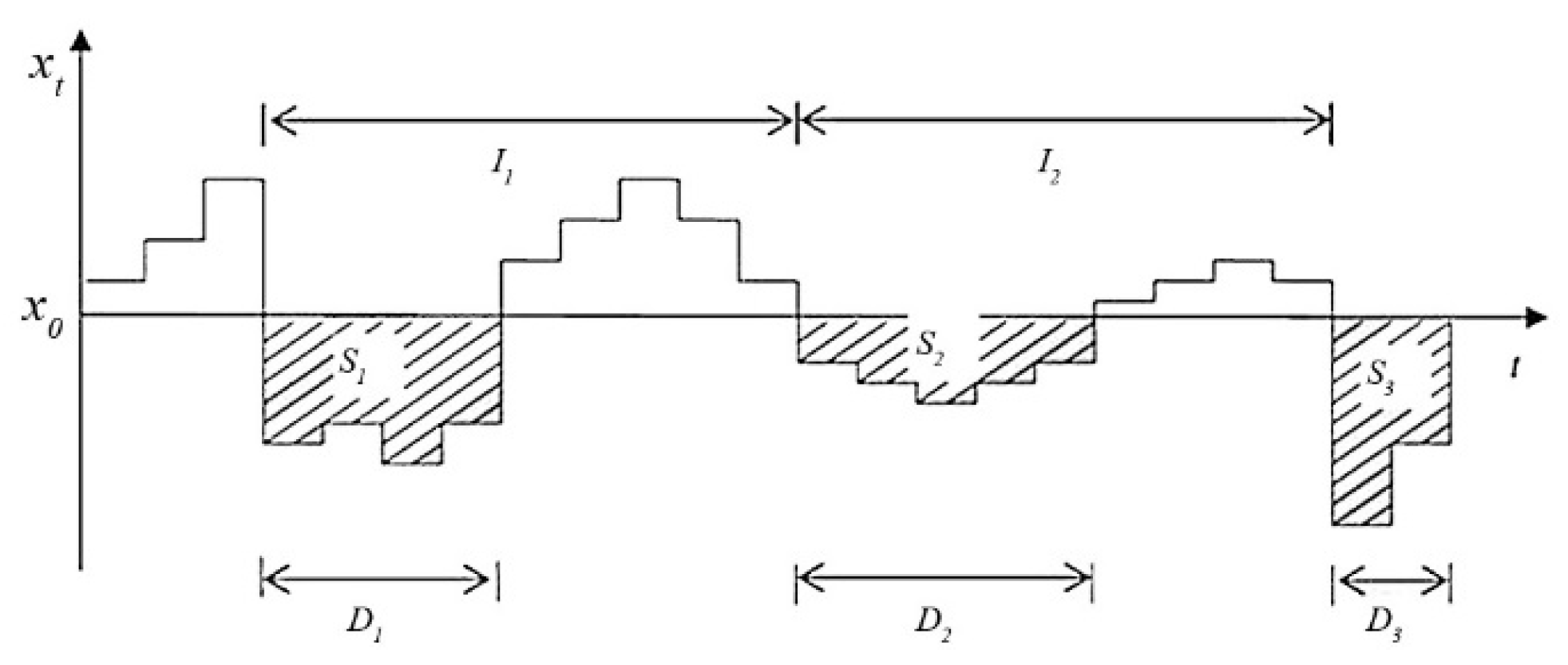
2.2. Drought Definition Using the Run Theory

This study qualitatively defines the hydrological drought (hereafter referred to as “drought”) as a significant decrease in the availability of streamflow in the river. Quantitatively, drought was defined using the run theory, which allows us to calculate drought duration, severity, and arrival time [61,62]. Thus, drought can be defined as the time when a hydro-meteorological time series${\text{ x}}_{\mathrm{t}}$ falls below the truncation level${\text{ x}}_0\text{ and }$that represents a hydro-meteorological event (Figure 2).

Drought events are based on the truncation level, so the selection of the level is one of the important issues for proper drought analysis. Generally, the mean value of streamflow has been widely used as the truncation level [63,64,65,66,67,68]. However, the Sacramento River streamflow shows high variability, between 5.13 and 51.65 MAF, so a median value of annual streamflow was regarded as a more reliable truncation level in this study.

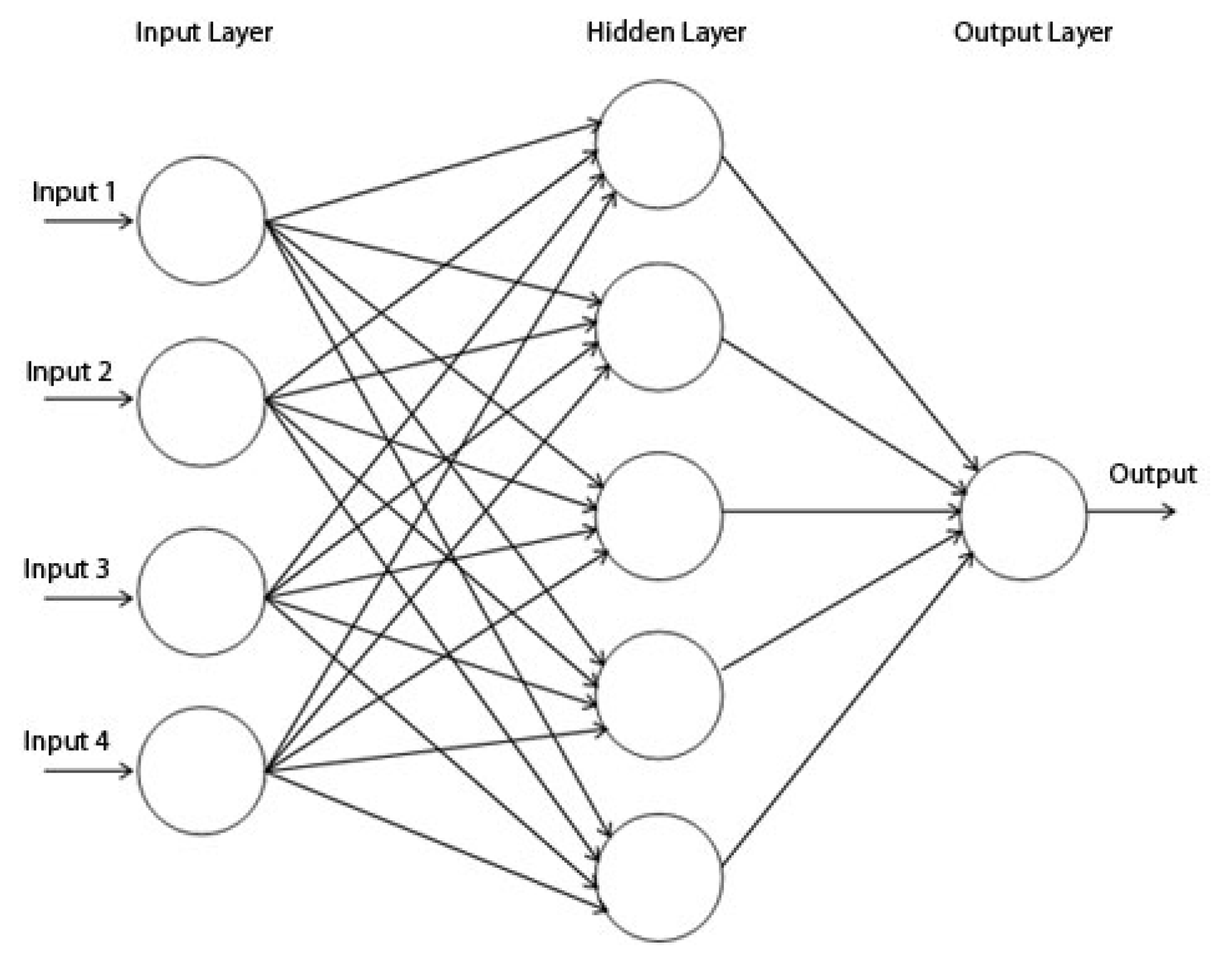
2.3. Artificial Neural Network

The factors that influence annual hydro-meteorological behavior can be roughly classified into four groups: (i) atmospheric-climatic; (ii) geologic-geomorphic; (iii) soil-vegetation; and (iv) runoff-channel factors [69]. Tree-ring widths in a trunk of a tree are also influenced by atmospheric-climatic and soil-vegetation factors, such as precipitation, evapotranspiration, and soil moisture. This indicates that an appropriate modeling technique and tree rings that have a correlation with atmospheric-climatic factors can be used to reconstruct annual streamflow, and this study employed an Artificial Neural Network (ANN) model. ANN mimics the structure and functions of a biological neural system, in which neurons are connected through nodes [70]. After the perceptron was proposed to categorize information patterns [71], ANNs have been widely used to recognize nonlinear relationships between different variables. The ANN used in this study was comprised of three layers: the input layer that represents observed streamflow data, the output layer that produces simulated streamflow, and the hidden layer that is constituted by a network of neurons that are trained to recognize patterns from observations (Figure 3).

The back-propagation algorithm was used to train the network through the adjustment of connection strength to learn about the error and optimize the neurons. It calculates the error function with respect to all the weights in the network and the gradient of error functions is fed into the optimization technique, which attempts to minimize the error of the network. Hence, the selection of back-propagation algorithm is one of the challenges when using a neural network [72]. The Levenberg–Marquardt–QNBP algorithm was selected as the back-propagation algorithm, because it is known to work well for non-linear problems, such as those related to meteorological and hydrological data [73]. Also, the number of hidden layers, which can be optimized by a trial and error method, is important for a proper network. The ANN model used in this study has six hidden layers that are optimized. One of the advantages of ANN is that it can be used as an alternative modeling technique when the data show non-linearity, which may cause error with a linear technique [74]. The tree-ring data in California and Oregon have autocorrelation and lagged-correlation characteristics [75], so ANN was employed as an alternative to reconstruct streamflow using tree-ring data. More details on ANN and the back-propagation algorithm can be found in Basheer and Hajmeer [76].

2.4. Drought Frequency Analysis Based on Copula

Unlike precipitation or flood occurrence, drought shows a different statistical behavior for a different duration [62]. Considering drought duration and severity as mutually related variables, the copula method has been employed to capture the dependence between them [47,77]. For a probability distribution $F\left(x_1,\dots , x_n\right)$, which has n-dimensional marginal distributions $F_1\left(x_1\right),\dots ,F_n\left( x_n\right)$, the copula function C that satisfies the relationship between marginal variables can be expressed as:

$$F\left(x_1,\dots ,x_n\right)=C(F_1\left(x_1\right),\dots ,F_n\left(x_n\right))={ \mathsf{\psi }}_{\alpha }{}^{-1} \left( {\mathsf{\psi }}_{\alpha }\left(F_1\left(x_1\right)\right)+\dots +{\mathsf{\psi }}_{\mathsf{\alpha }}\left(F_n\left(x_n\right)\right)\right)$$

(1)

$$1/T= E\left(L\right) / \left\{1-F_1-F_2\dots ,F_n+C\left(F_1,F_2,\dots ,F_n\right)\right\}$$

(2)

where ${\mathsf{\psi }}_{\alpha }$ denotes the generating function; ${\mathsf{\psi }}_{\alpha }{}^{-1}$is the pseudo-inverse of that function, which differs with the copula family; T denotes the return period; and E(L) is the interval between events. Unlike univariate frequency analysis, bivariate frequency indicates the probability that the phenomenon under study occurs if and only if a prior condition takes place. There are several types of copula functions, but the Archimedean copula family, which allows for greater flexibility and simplicity of use, is more commonly used in hydrology [78]. From the Archimedean copula family, the Clayton, Gumbel, and Frank copulas were employed and their functions are given in

Table 2. Bivariate Archimedean copula family: $C$ is the copula function, t denotes the drought event, $\alpha$ is the copula parameter, and F₁ and F₂ denote cumulative distribution function of each variable [79].

Copula Family	Copula func., $C(F_1\left(x_1\right),F_2\left(x_2\right))$	Generator func., ${\mathsf{\psi }}_{\mathit{\alpha }}\left(\mathit{t}\right)$	Parameter (α)
Clayton	$\left(\max \left\{F_1{\left(x_1\right)}^{-1}+ F_2{\left(x_2\right)}^{-1}-1;0\right\}\right)$	$\frac{1}{\mathsf{\alpha }}\left(t^{-\alpha }-1\right)$	$\mathsf{\alpha }\in \left[-1,\infty \right]$
Frank	$\frac{-1}{\mathsf{\alpha }}\text{log}\left(1+\frac{\left(\exp \left(-\alpha F_1\left(x_1\right)\right)-1\right)(\text{exp}\left(-\alpha F_2\left(x_2\right)-1\right) }{\exp \left(-\alpha \right)-1}\right)$	$-\log \left(\frac{\exp \left(-\alpha t\right)-1 }{\exp \left(-\alpha \right)-1}\right)$	$\mathsf{\alpha }\in \left[ℛ\right]$
Gumbel	$\exp \left(-{\left({\left(-\text{log}(F_1\left(x_1\right)\right)}^{\alpha }+ {\left(-\text{log}(F_1\left(x_1\right)\right)}^{\alpha }\right)}^{\frac{1}{\alpha }}\right)$	$-\log {\left(t\right)}^{\alpha }$	$\mathsf{\alpha }\in \left[1,\infty \right]$

.

3. Results and Discussion

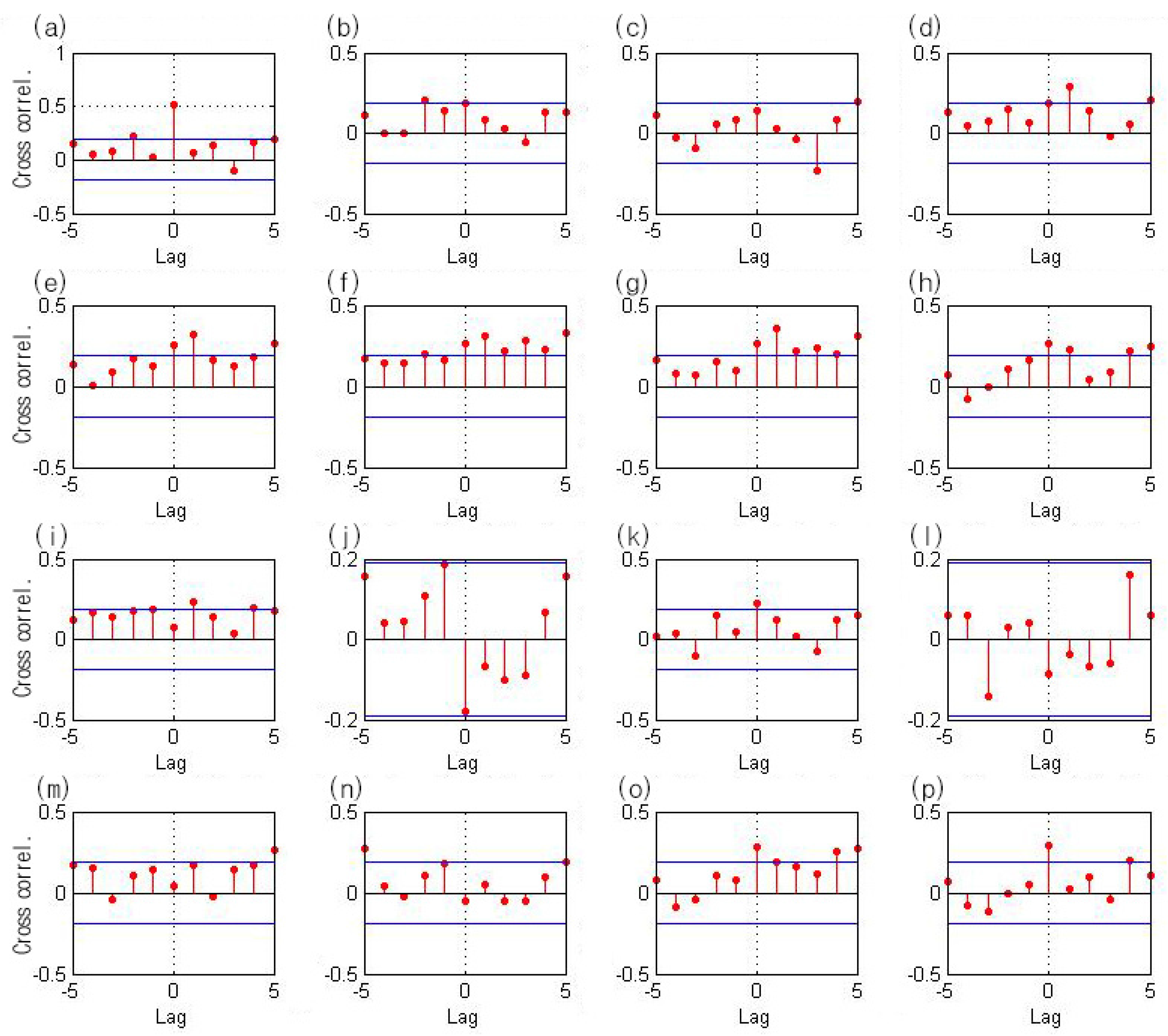
3.1. Tree-Ring Data Screening

Appropriate tree rings, which have correlation with atmospheric-climatic factors, can be used as the predictor for annual streamflow. Therefore, selection of the appropriate input for the ANN model was one of the challenges in this study. Generally, a trial and error method with different input variables is employed, but it can lead to the poor performance of neural networks [80,81]. Alternatively, cross correlation coefficients were employed to select appropriate inputs in this study in the same way as Meko et al. [75].

Seven tree-rings indices showed correlation with streamflow (Figure 4), including Antelope Lake (Pinus Jeffreyi and Pinus Ponderosa), Felkner Ridge, Frederick Butte, Lemon Canyon, Piute Mountain, and Sorrel Peak; four tree rings had correlation with a one-year time-lag, including Dalton Reservoir, Hager Basin Reservoir and Antelope Lake (Pinus Jeffreyi and Pinus Ponderosa), as shown in Figure 4 and Figure 5. Hence, nine tree rings were selected as predictors for the ANN model (two tree-rings were overlapped in zero-lagged and one-year lagged). Also, four tree-rings, which had one-year time-lag correlation (Antelope with Pinus Jeffreyi and Pinus Ponderosa, Dalton Reservoir, and Hager Basin Reservoir), are located on the nearby lake or reservoir. Therefore, it seems that the groundwater level or soil moisture influenced tree ring width, but there are no clues to estimate the correlation between them and further studies are thus needed. These nine tree-ring data points composed the input dataset for the ANN model.

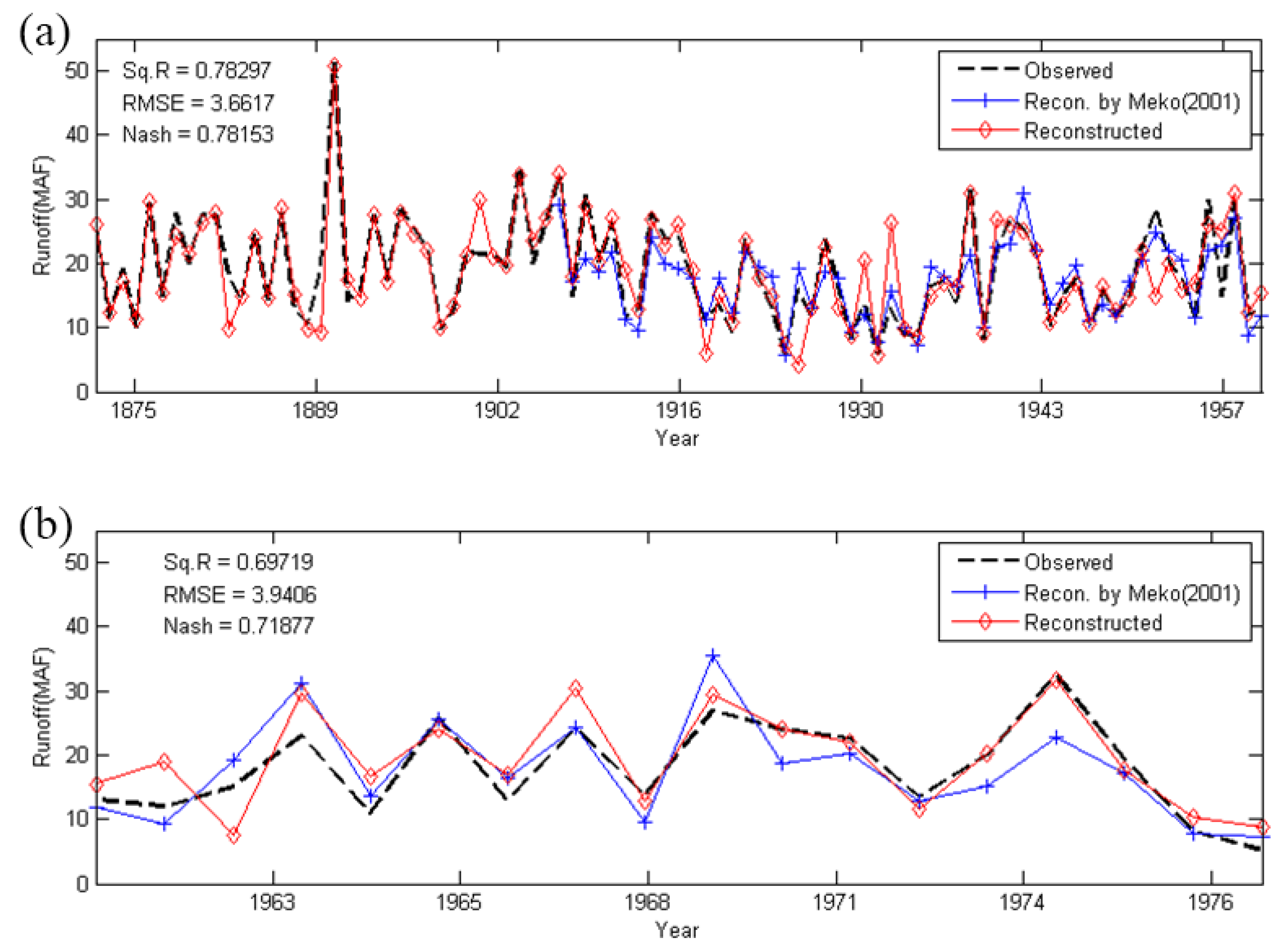
3.2. Reconstructed ANN Model Calibration and Validation

The ANN model had six hidden layers that were determined by trial and error and was established with selected predictors. The Sacramento streamflow data were divided into calibration period (1872 to 1957) and validation period (1958 to 1977). To evaluate the results of calibration and validation, R² and RMSE [82], and the Nash–Sutcliffe model efficiency coefficient [83] were computed. The RMSE describes a measure of average error in prediction and R² and Nash–Sutcliffe model efficiency coefficient have been widely used to assess the predictive performance of models [84]. The calibration and validation results with selected predictors are shown in Figure 6.

The ANN model showed relatively high values of evaluation measures, with R², RMSE, and Nash–Sutcliffe efficiency of 0.78, 3.66, and 0.78 in the calibration and 0.70, 3.94, and 0.72 in the validation period, respectively. Thus, the reconstructed streamflow, based on the ANN model and selected predictor, could be used as the reconstruction model. Also, it could be used for hydro-meteorological simulations. The variability of each period was 5.74 to 51.64 MAF in the calibration period and 5.13 to 32.5 MAF in the validation period.

The reconstructed streamflow using the selected predictor (nine tree rings) is shown in Figure 7 and the basic statistics are shown in

Table 3. Basic statistics of observed and reconstructed streamflow.

Period	Mean (MAF)	Median (MAF)	Standard Deviation (MAF)	Skewness
Observed (1872–1977)	18.9	17.6	7.8	0.8
Reconstructed (1560–1871)	20.4	19.8	9.6	0.6

, with an average of 18.9 MAF observed and 20.4 MAF of reconstructed streamflow.

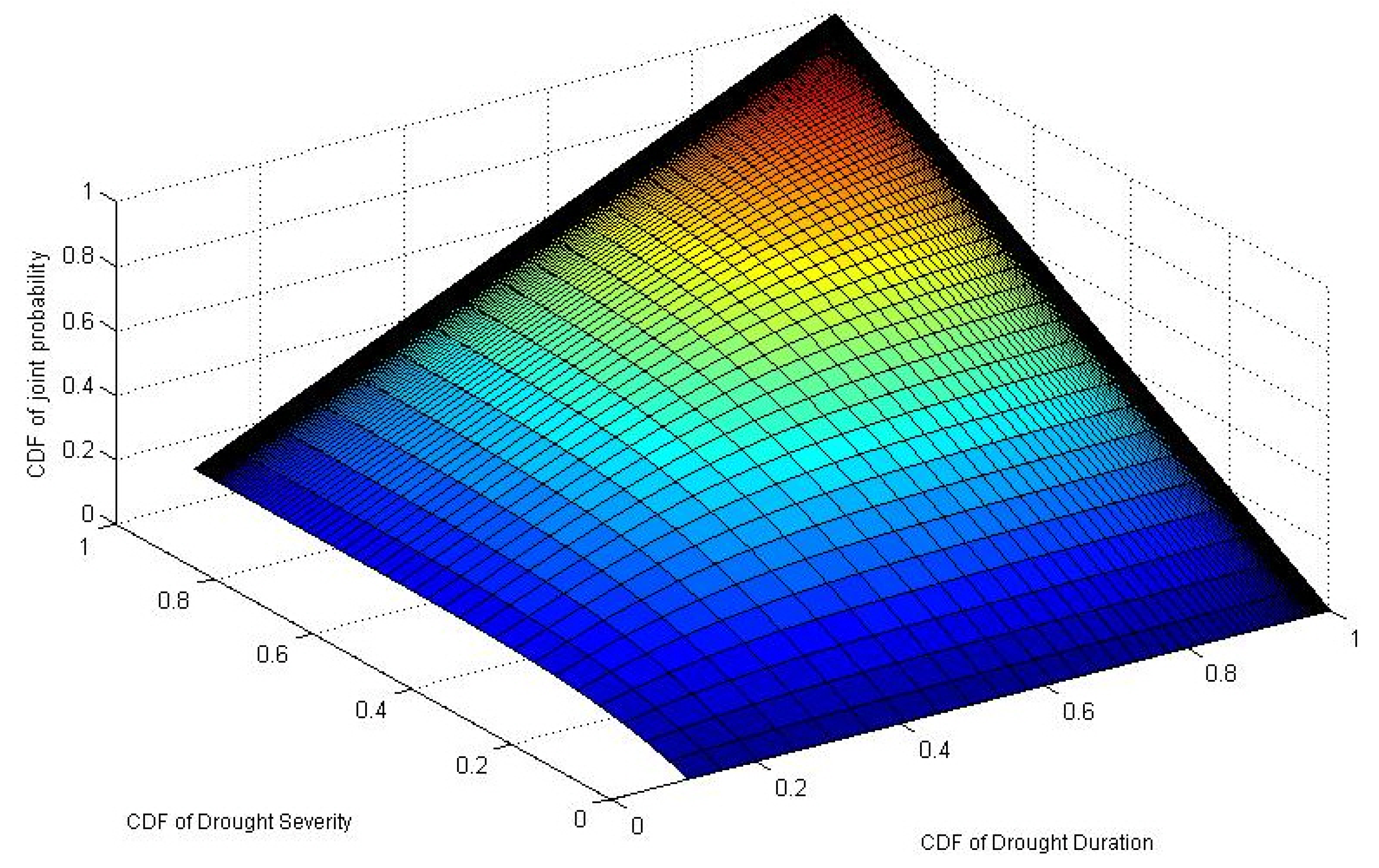
3.3. Bivariate Drought Analysis and Discussion

Before drought analysis based on reconstructed streamflow, the truncation level that defines the relevant streamflow level was determined to define hydrological drought from the streamflow series. The median value of annual streamflow, which was 19.4 MAF, was employed as the truncation level to define hydrological droughts for the Sacramento River basin and results are shown in Figure 8. In total, 96 droughts occurred during the period from 1560 to 1977. Their statistical characteristics were: median drought duration of about two years, average drought severity of about 15.8 MAF, and average drought arrival time of about 2.1 years during the 15th to 20th centuries. The longest drought duration estimated was 10 years and had 75.31 MAF during 1927 to 1936 (in the observation period), and the severest drought estimated was 76.17 MAF, which had an eight-year drought duration from 1582 to 1589 (in the reconstruction period).

For bivariate drought frequency analysis with the copula function, marginal distributions of drought variables (duration and severity) were derived. The drought duration was found to have an “exponential” distribution, if treated as a continuous random variable [34]. Also, the drought severity was found to have a “gamma” distribution with 95% confidential level with the PPCC (probability plot correlation coefficient; [85]) distribution goodness of fit test. Then, parameters of the Archimedean family copulas (Frank, Clayton, and Gumbel) were estimated by the method of moments according to their relationship between copula parameter and Kendall’s tau [86], which has been found adequate for estimating parameters for small sample sizes [78].

The minimum quadratic distance (L²) between the empirical and theoretical values of the $K$ criterion, which describes the most appropriate copula [78], was calculated for each copula. As shown in Figure 9, the Frank copula, which generally fitted well throughout (L² = 0.023), was selected for bivariate drought analysis for the Sacramento River. The Frank copula parameter was estimated as 8.03, and the bivariate joint probability of drought for the Sacramento River basin was described as:

$$F\left( F_d, F_s\right)=-\frac{1}{8.03}\text{log}\left(1+\frac{\left(\exp \left(-8.03 F_d\left(t\right)\right)-1\right)(\text{exp}\left(-8.03 F_s\left(t\right)-1\right) }{\exp \left(-8.03\right)-1}\right)$$

(3)

where, $F_d\left(t\right)$ and $F_s\left(t\right)$ are the cumulative distribution functions of drought duration and severity. Figure 10 shows the joint CDF of the Sacramento River basin drought.

The return period is described as the average time of occurrence of events with the threshold intensity. The bivariate return period can be divided into the exceedance probabilities of both the drought duration and severity [62]. The copula-based return period with the average inter-arrival of occurrences ($E\left(L\right)$), which was 2.1 years, can be defined as:

$$T_{return period}= \frac{2.1}{P\left(D>d \& S>s\right)}=\frac{2.1}{1-F_D\left(d\right)-F_S\left(s\right)+C\left(F_D\left(d\right),F_S\left(s\right)\right)}$$

(4)

Therefore, the duration and severity of droughts can be expressed in terms of the same return period, which can be illustrated in each “return period plot”, as shown in Figure 11.

The drought event and return period plot in Figure 11 shows the hydrological drought pattern of the Sacramento River basin. Overall, the drought duration and severity seemed to have a positive correlation with each other. To identify the correlation between drought duration and severity, Pearson’s linear correlation coefficient, Kendall’s rank correlation coefficient (τ), and Spearman’s rank correlation coefficient (ρ) were found to be 0.92, 0.73, and 0.85, respectively. Also, the severity of two-year duration drought showed higher variability than did the three-year duration drought. Strong correlation between drought characteristics and higher variability of the two-year drought was the basis for the copula method, especially higher variability of severity or larger statistical irregularity than other durations for the same return period in the univariate frequency analysis [62]. Hence, the copula method would be expected to be more reliable for drought analysis for the Sacramento River basin. Furthermore, California has a 22.4 MAF mean annual runoff and used 5.2 MAF annually to supply the southern area [87]. So, a drought that becomes over 17.2 MAF will cause the shortage of water supply and is equivalent to approximately a 20-year return period with a two-month duration (median value of drought duration) based on the return period plot in Figure 11. Therefore, any return period that causes an actual water shortage could be the appropriate critical level of drought. Also, the return period plot in Figure 11 can be used as elementary data for water resources planning. For instance, if a decision maker or agency determined a three-year design drought for a dam or reservoir to be having a 20-year return period, then its deficiency would be about $11.1\times {10}^9{\text{ m}}^3$ (27.0 MAF), and it could be the target storage volume for water resources planning.

Most of the droughts that occurred during the last five centuries did not have more than a 50-year return period, and just six droughts showed 100-year or longer return periods. These high return period events are one of the limitations of the study; for instance, the drought from 1927 to 1936 years, the longest and severest drought in historical data [88], with a 10-year duration and 75.31 MAF severity, which equated to a $9.26\times {10}^9{\text{ m}}^3$ streamflow deficiency per year, had approximately a 7500-year return period. That extreme return period was due to the Frank copula and sample size, which shows some bias in high quantile (high return period) events in Figure 9, so it could have overestimated the return period [89], and the number of drought events with high quantiles is also limited. Droughts that have high quantiles or extreme return periods depend significantly on the fitted copula function. Therefore, further studies are needed for generally well-fitted copulas throughout, and also for carefully considering the use of the return period plot in water resources planning.

4. Conclusions

This study reconstructed the past streamflow of the Sacramento River based on the ANN and tree-ring data, and bivariate drought frequency was analyzed using the Archimedean copula. Results of this study can be summarized as follows:

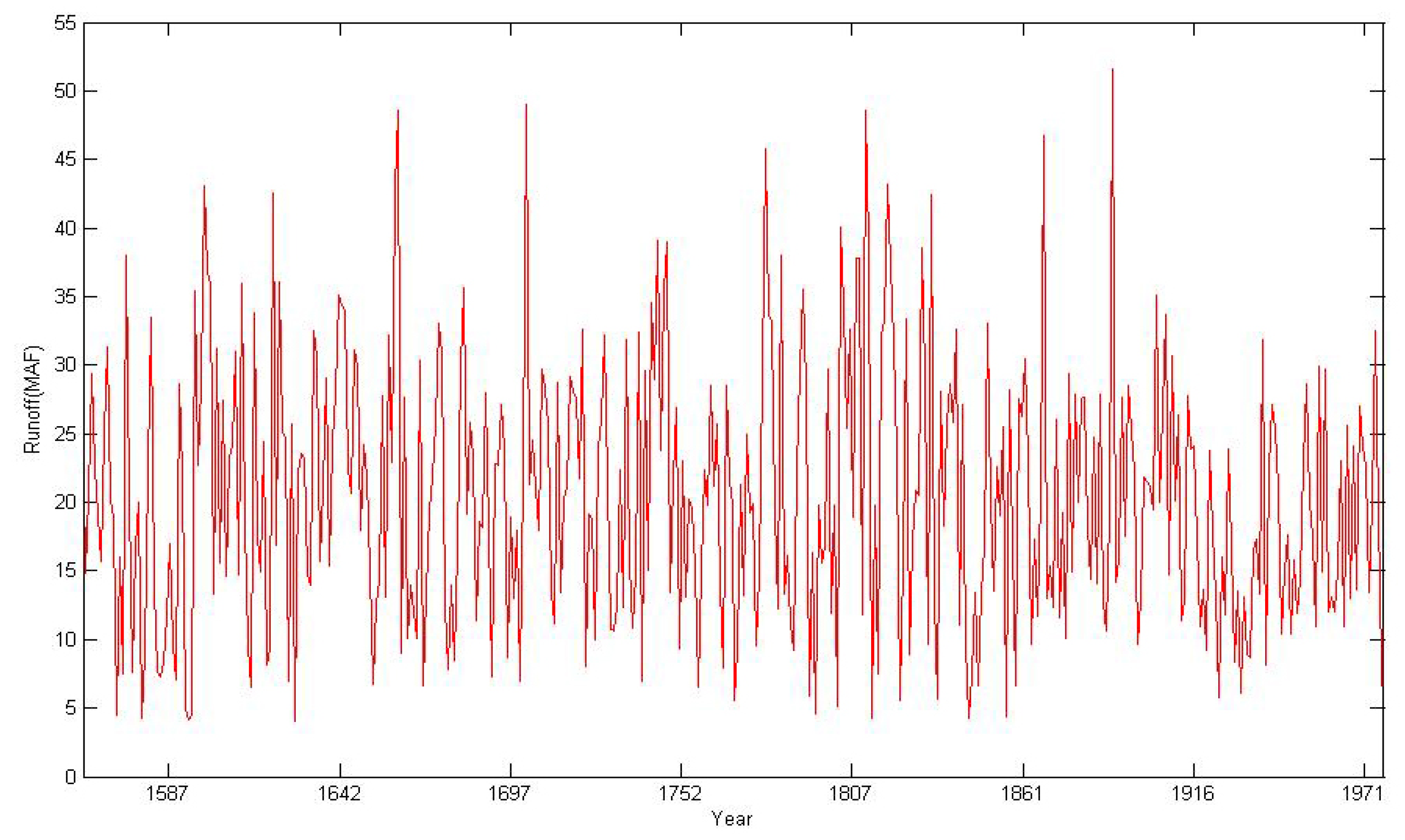
• The past streamflow for the period from 1560 to 1871 is reconstructed with the ANN model and tree-ring data, which was found to be the appropriate predictor. As shown by calibration and validation results from 1872 to 1977, the R² and Nash values are 0.7 or higher. It is therefore concluded that the ANN model reconstructs streamflow of the Sacramento River satisfactorily.
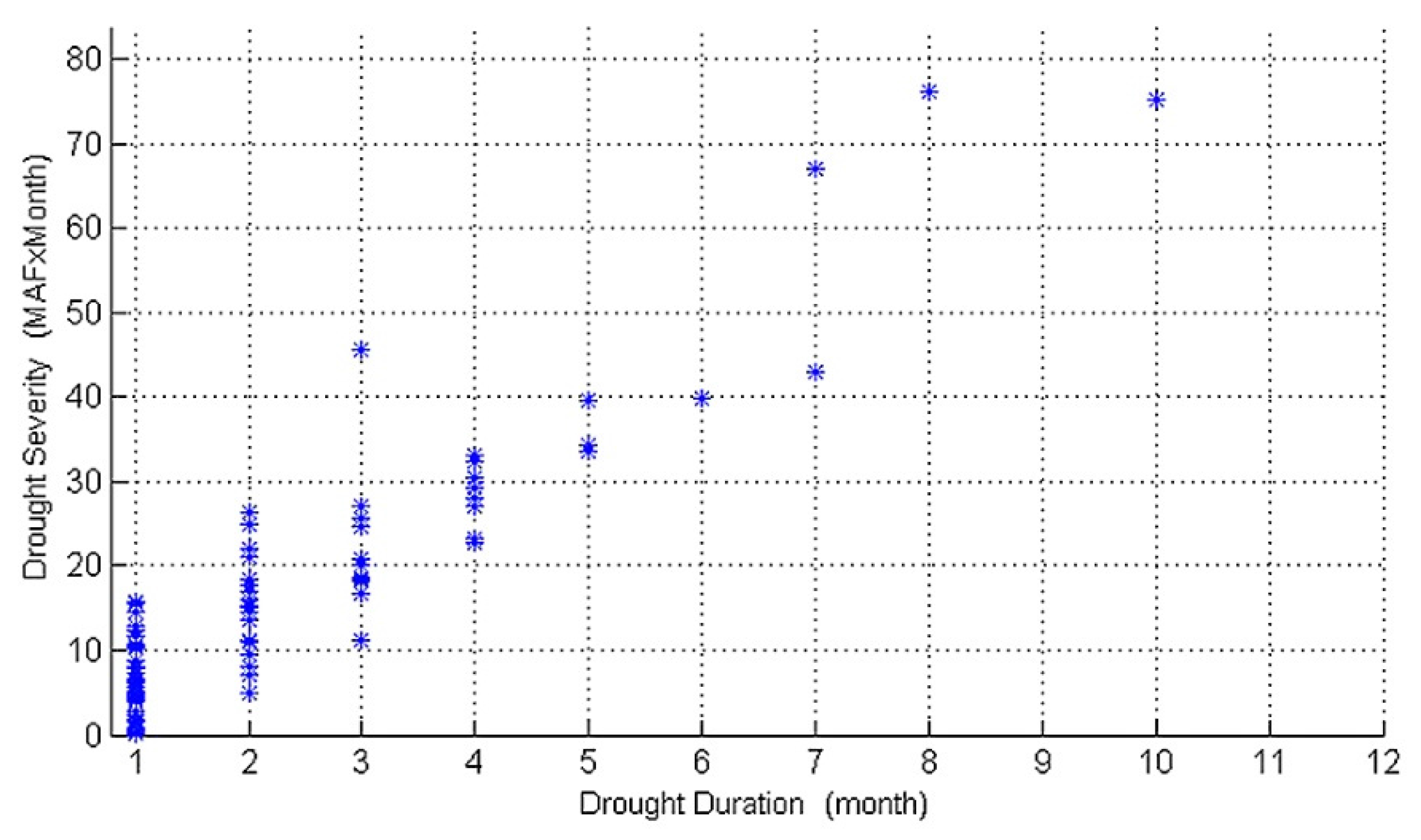
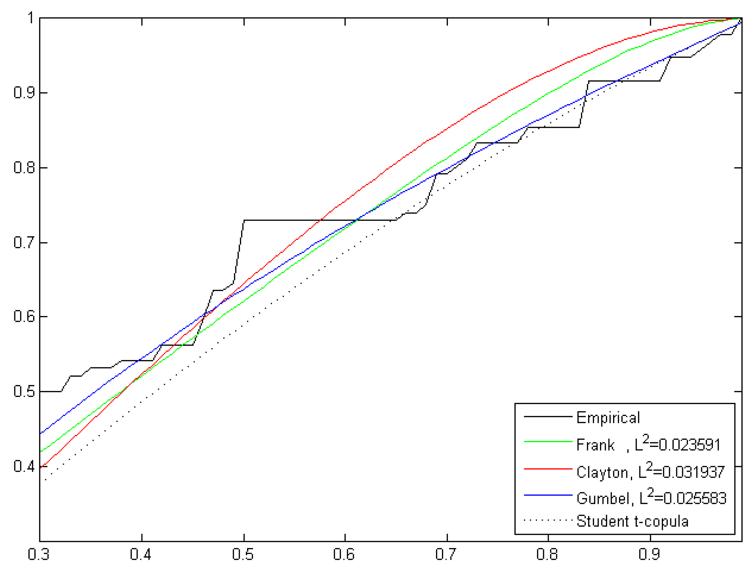
• Drought characteristics in the Sacramento River basin have strong correlation with each other. The Archimedean copula is found to be appropriate for bivariate drought frequency analysis.
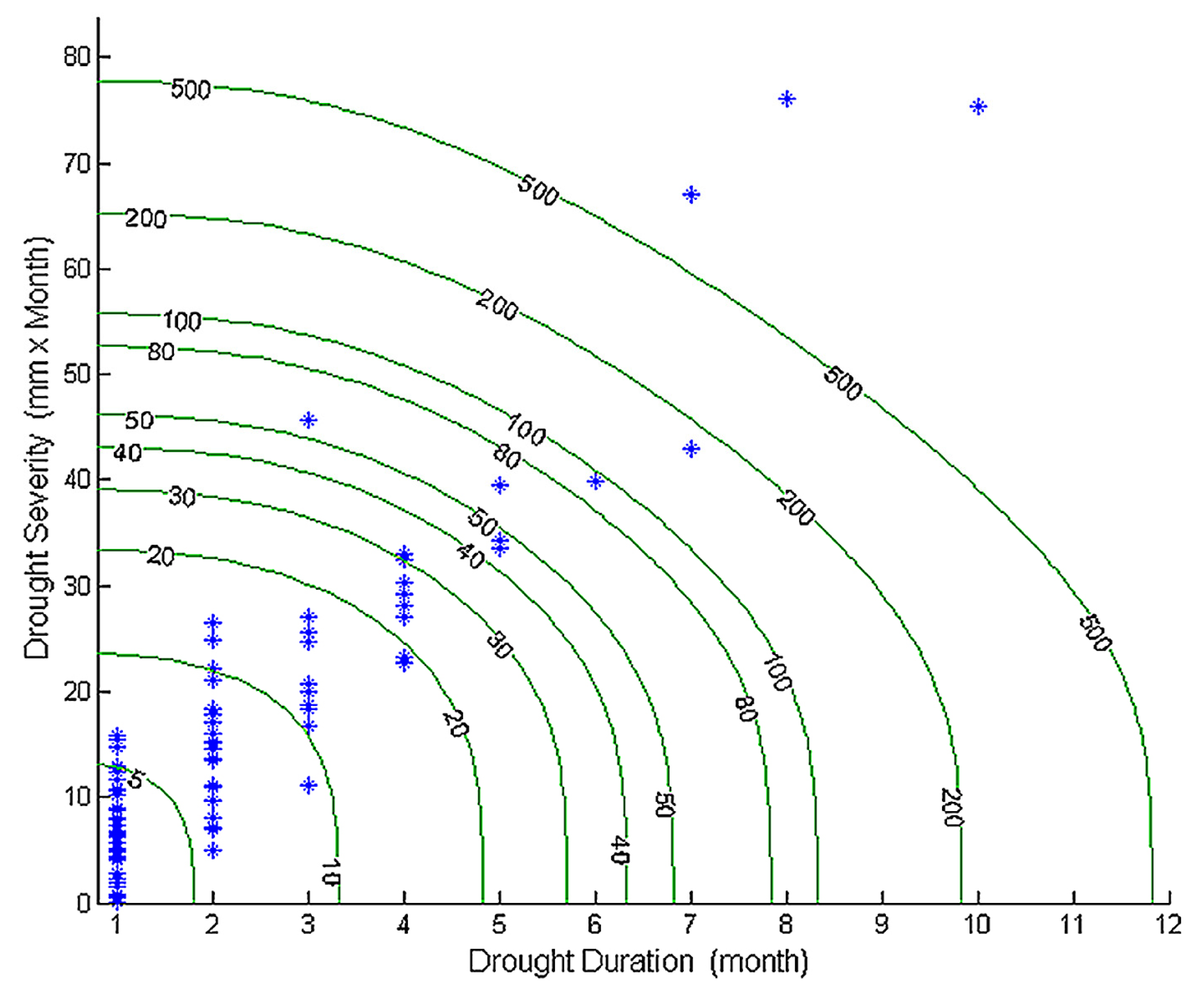
• It is shown that a drought with a 20-year return period or longer will cause actual water shortages in the perspective of water supply to the southern California area. Hence, it could be considered an appropriate critical level of droughts for actual water shortages.

References

1. Wang, B.; Jhun, J.G.; Moon, B.K. Variability and singularity of Seoul, South Korea, rainy season (1778–2004). J. Clim. 2007, 20, 2572–2580. [Google Scholar] [CrossRef]
2. Mun, J.W.; Lee, D.Y. Tree-ring data application for drought mitigation. J. Korean Soc. Hazard Mitig. 2011, 11, 70–78. (In Korean) [Google Scholar]
3. Kim, H.S.; Hwang, S.H.; Kim, J.H. Reconstruction of River Flows Using Tree-Ring Series and Neural Network. J. Korean Soc. Civ. Eng. 1998, 18, 583–589. [Google Scholar]
4. Ferguson, C.W. Bristlecone Pine: Science and Esthetics A 7100-year tree-ring chronology aids scientists; old trees draw visitors to California mountains. Science 1968, 159, 839–846. [Google Scholar] [CrossRef] [PubMed]
5. Fritts, H.C. Tree-ring analysis: A tool for water resources research. Eos Trans. Am. Geophys. Union 1969, 50, 22–29. [Google Scholar] [CrossRef]
6. Fritts, H.C. Tree Rings and Climate; Academic Press Inc.: New York, NY, USA, 1976. [Google Scholar]
7. Hughes, M.K.; Xiangding, W.; Xuemei, S.; Garfin, G.M. A preliminary reconstruction of rainfall in north-central China since AD 1600 from tree-ring density and width. Quat. Res. 1994, 42, 88–99. [Google Scholar] [CrossRef]
8. Díaz, S.C.; Touchan, R.; Swetnam, T.W. A tree-ring reconstruction of past precipitation for Baja California Sur, Mexico. Int. J. Climatol. 2001, 21, 1007–1019. [Google Scholar] [CrossRef]
9. Cleaveland, M.K.; Stahle, D.W.; Therrell, M.D.; Villanueva-Diaz, J.; Burns, B.T. Tree-ring reconstructed winter precipitation and tropical teleconnections in Durango, Mexico. Clim. Chang. 2003, 59, 369–388. [Google Scholar] [CrossRef]
10. Gray, S.T.; Fastie, C.L.; Jackson, S.T.; Betancourt, J.L. Tree-ring-based reconstruction of precipitation in the Bighorn Basin, Wyoming, since 1260 AD. J. Clim. 2004, 17, 3855–3865. [Google Scholar] [CrossRef]
11. Liu, Y.; Cai, Q.; Shi, J.; Hughes, M.K.; Kutzbach, J.E.; Liu, Z.; An, Z. Seasonal precipitation in the south-central Helan Mountain region, China, reconstructed from tree-ring width for the past 224 years. Can. J. For. Res. 2005, 35, 2403–2412. [Google Scholar] [CrossRef]
12. Liu, Y.; Ma, L.; Leavitt, S.W.; Cai, Q.; Liu, W. A preliminary seasonal precipitation reconstruction from tree-ring stable carbon isotopes at Mt. Helan, China, since AD 1804. Glob. Planet. Chang. 2004, 41, 229–239. [Google Scholar] [CrossRef]
13. Schneuwly, D.M.; Stoffel, M. Tree-ring based reconstruction of the seasonal timing, major events and origin of rockfall on a case-study slope in the Swiss Alps. Nat. Hazards Earth Syst. Sci. 2008, 8, 203–211. [Google Scholar] [CrossRef]
14. Frank, D.; Esper, J. Characterization and climate response patterns of a high-elevation, multi-species tree-ring network in the European Alps. Dendrochronologia 2005, 22, 107–121. [Google Scholar] [CrossRef]
15. Cook, E.R.; Jacoby, G.C. Tree-ring-drought relationships in the Hudson Valley, New York. Science 1977, 198, 399–401. [Google Scholar] [CrossRef] [PubMed]
16. Stockton, C.W.; Meko, D.M. Drought Recurrence in the Great Plains as Reconstructed from Long-Term Tree-Ring Records. J. Clim. Appl. Meteorol. 1983, 22, 17–29. [Google Scholar] [CrossRef]
17. Graumlich, L.J. Precipitation variation in the Pacific Northwest (1675–1975) as reconstructed from tree rings. Ann. Assoc. Am. Geogr. 1987, 77, 19–29. [Google Scholar] [CrossRef]
18. Till, C.; Guiot, J. Reconstruction of precipitation in Morocco since 1100 AD Based on Cedrus atlantica tree-ring widths. Quat. Res. 1990, 33, 337–351. [Google Scholar] [CrossRef]
19. Meko, D.; Stockton, C.W.; Boggess, W.R. The Tree-ring Record of Severe Sustained Drought. J. Am. Water Resour. Assoc. 1995, 31, 789–801. [Google Scholar] [CrossRef]
20. Stahle, D.W.; Cook, E.R.; Cleaveland, M.K.; Therrell, M.D.; Meko, D.M.; Grissino-Mayer, H.D.; Luckman, B.H. Tree-ring data document 16th century mega drought over North America. EOS Trans. Am. Geophys. Union 2000, 81, 121–125. [Google Scholar] [CrossRef]
21. Raffalli-Delerce, G.; Masson-Delmotte, V.; Dupouey, J.L.; Stievenard, M.; Breda, N.; Moisselin, J.M. Reconstruction of summer droughts using tree-ring cellulose isotopes: A calibration study with living oaks from Brittany (western France). Tellus B 2004, 56, 160–174. [Google Scholar] [CrossRef]
22. Li, J.; Gou, X.; Cook, E.R.; Chen, F. Tree-ring based drought reconstruction for the central Tien Shan area in northwest China. Geophys. Res. Lett. 2006, 33. [Google Scholar] [CrossRef]
23. Li, J.; Chen, F.; Cook, E.R.; Gou, X.; Zhang, Y. Drought reconstruction for north central China from tree rings: The value of the Palmer drought severity index. Int. J. Climatol. 2007, 27, 903–909. [Google Scholar] [CrossRef]
24. Tian, Q.; Gou, X.; Zhang, Y.; Peng, J.; Wang, J.; Chen, T. Tree-ring based drought reconstruction (AD 1855–2001) for the Qilian Mountains, northwestern China. Tree Ring Res. 2007, 63, 27–36. [Google Scholar] [CrossRef]
25. Mishra, A.K.; Singh, V.P. Drought modeling—A review. J. Hydrol. 2011, 403, 157–175. [Google Scholar] [CrossRef]
26. Agüero, J.D.L.C.; Rodríguez, F.J.G. Morphometric stock structure of the Pacific sardine Sardinops sagax (Jenyns, 1842) off Baja California, Mexico. In Morphometrics; Springer: Berlin, Germany; Heidelberg, Germany, 2004. [Google Scholar]
27. Stockton, C.W.; Meko, D.M. A long-term history of drought occurrence in western United States as inferred from tree rings. Weatherwise 1975, 28, 244–249. [Google Scholar] [CrossRef]
28. Gray, S.T.; Betancourt, J.L.; Fastie, C.L.; Jackson, S.T. Patterns and sources of multidecadal oscillations in drought-sensitive tree-ring records from the central and southern Rocky Mountains. Geophys. Res. Lett. 2003, 30. [Google Scholar] [CrossRef]
29. Helama, S.; Meriläinen, J.; Tuomenvirta, H. Multicentennial megadrought in northern Europe coincided with a global El Niño–Southern Oscillation drought pattern during the Medieval Climate Anomaly. Geology 2009, 37, 175–178. [Google Scholar] [CrossRef]
30. Ropelewski, C.F.; Halpert, M.S. North American precipitation and temperature patterns associated with the El Niño/Southern Oscillation (ENSO). Monthly Weather Rev. 1986, 114, 2352–2362. [Google Scholar] [CrossRef]
31. Davi, N.K.; Jacoby, G.C.; D’Arrigo, R.D.; Baatarbileg, N.; Jinbao, L.; Curtis, A.E. A tree-ring-based drought index reconstruction for far-western Mongolia: 1565–2004. Int. J. Climatol. 2009, 29, 1508–1514. [Google Scholar] [CrossRef]
32. Touchan, R.; Funkhouser, G.; Hughes, M.K.; Erkan, N. Standardized precipitation index reconstructed from Turkish tree-ring widths. Clim. Chang. 2005, 72, 339–353. [Google Scholar] [CrossRef]
33. Liang, E.; Shao, X.; Liu, H.; Eckstein, D. Tree-ring based PDSI reconstruction since AD 1842 in the Ortindag Sand Land, east Inner Mongolia. Chin. Sci. Bull. 2007, 52, 2715–2721. [Google Scholar] [CrossRef]
34. Shiau, J.T. Fitting drought duration and severity with two-dimensional copulas. Water Resour. Manag. 2006, 20, 795–815. [Google Scholar] [CrossRef]
35. Chbouki, N. Spatio-Temporal Characteristics of Drought as Inferred from Tree-Ring Data in Morocco. Ph.D. Thesis, University of Arizona, Tucson, AZ, USA, 1992. [Google Scholar]
36. Shiau, J.T.; Modarres, R. Copula-based drought severity-duration-frequency analysis in Iran. Meteorol. Appl. 2009, 16, 481–489. [Google Scholar] [CrossRef]
37. Rajsekhar, D.; Singh, V.P.; Mishra, A.K. Multivariate drought index: An information theory based approach for integrated drought assessment. J. Hydrol. 2015, 526, 164–182. [Google Scholar] [CrossRef]
38. Hao, Z.; AghaKouchak, A. Multivariate standardized drought index: A parametric multi-index model. Adv. Water Resour. 2013, 57, 12–18. [Google Scholar] [CrossRef]
39. Brown, J.F.; Wardlow, B.D.; Tadesse, T.; Hayes, M.J.; Reed, B.C. The Vegetation Drought Response Index (VegDRI): A new integrated approach for monitoring drought stress in vegetation. GISci. Remote Sens. 2008, 45, 16–46. [Google Scholar] [CrossRef]
40. Tadesse, T.; Wardlow, B.D.; Brown, J.F.; Svoboda, M.D.; Hayes, M.J.; Fuchs, B.; Gutzmer, D. Assessing the vegetation condition impacts of the 2011 drought across the US Southern Great Plains using the Vegetation Drought Response Index (VegDRI). J. Appl. Meteorol. Climatol. 2015, 54, 153–169. [Google Scholar] [CrossRef]
41. Alley, W.M. The Palmer Drought Severity Index: Limitations and assumptions. J. Clim. Appl. Meteorol. 1984, 23, 1100–1109. [Google Scholar] [CrossRef]
42. Shafer, B.A.; Dezman, L.E. Development of a Surface Water Supply Index (SWSI) to assess the severity of drought conditions in snowpack runoff areas. In Proceedings of the Western Snow Conference, Reno, Nevada, April 1982; pp. 164–175.
43. Valipour, M. Use of surface water supply index to assessing of water resources management in Colorado and Oregon. Adv. Agric. 2013, 3, 631–640. [Google Scholar]
44. González, J.; Valdés, J.B. Bivariate drought recurrence analysis using tree ring reconstructions. J. Hydrol. Eng. 2003, 8, 247–258. [Google Scholar] [CrossRef]
45. Vangelis, H.; Spiliotis, M.; Tsakiris, G. Drought severity assessment based on bivariate probability analysis. Water Resour. Manag. 2011, 25, 357–371. [Google Scholar] [CrossRef]
46. Murtin, C.M.; Murtin, F. Education Inequalities among World Citizens: 1870–2000. 2006. Working Paper. Available online: http://www.eea-esem.com/files/papers/EEA-ESEM/2006/2780/EducationInequality.pdf (accessed on 21 March 2016).
47. Sklar, A. Fonctions de Repartition `a n Dimensions et Leura Marges; Publication de l’Institut de Statistique de l’Université de Paris: Paris, France, 1959; pp. 229–231. (In French) [Google Scholar]
48. Shiau, J.T.; Feng, S.; Nadarajah, S. Assessment of hydrological droughts for the Yellow River, China, using copulas. Hydrol. Process. 2007, 21, 2157–2163. [Google Scholar] [CrossRef]
49. Serinaldi, F.; Bonaccorso, B.; Cancelliere, A.; Grimaldi, S. Probabilistic characterization of drought properties through Copulas. Phys. Chem. Earth 2009, 34, 596–605. [Google Scholar] [CrossRef]
50. Song, S.; Singh, V.P. Meta-elliptical copulas for drought frequency analysis of periodic hydrologic data. Stoch Environ. Res. Risk Assess. 2010, 24, 425–444. [Google Scholar] [CrossRef]
51. Mirabbasi, R.; Anagnostou, E.N.; Fakheri-Fard, A.; Dinpashoh, Y.; Eslamian, S. Analysis of meteorological drought in northwest Iran using the Joint Deficit Index. J. Hydrol. 2013, 492, 35–48. [Google Scholar] [CrossRef]
52. Chen, L.; Singh, V.P.; Guo, S.; Mishra, A.K.; Guo, J. Drought Analysis Using Copulas. J. Hydrol. Eng. 2012, 18, 797–808. [Google Scholar] [CrossRef]
53. Vergni, L.; Todisco, F.L.; Mannocchi, F. Analysis of agricultural drought characteristics through a two-dimensional copula. Water Resour. Manag. 2015, 29, 2819–2835. [Google Scholar] [CrossRef]
54. Huang, S.; Huang, Q.; Chang, J.; Chen, Y.; Xing, L.; Xie, Y. Copulas-Based Drought Evolution Characteristics and Risk Evaluation in a Typical Arid and Semi-Arid Region. Water Resour. Manag. 2014, 29, 1489–1503. [Google Scholar] [CrossRef]
55. Reddy, M.J.; Singh, V.P. Multivariate modeling of droughts using copulas and meta-heuristic methods. Stoch. Environ. Rese. Risk Assess. 2014, 28, 475–489. [Google Scholar] [CrossRef]
56. Mishra, A.; Singh, V.P.; Desai, V. Drought characterization: A probabilistic approach. Stoch. Environ. Res. Risk Assess. 2009, 23, 41–55. [Google Scholar] [CrossRef]
57. Jacoby, G.C.; Cook, E.R. Past temperature variations inferred from a 400-year tree-ring chronology from Yukon Territory, Canada. Arct. Alp. Res. 1981, 13, 409–418. [Google Scholar] [CrossRef]
58. Grissino-Mayer, H.D.; Fritts, H.C. The International Tree-Ring Data Bank: An enhanced global database serving the global scientific community. Holocene 1997, 7, 235–238. [Google Scholar] [CrossRef]
59. Cook, E.R. A time series analysis approach to tree-ring standardization (Dendrochronology, Forestry, Dendroclimatology, Autoregressive process). Ph.D. Thesis, University of Arizona, Tucson, AZ, USA, 1985. [Google Scholar]
60. California Data Exchange Center. Available online: http://cdec.water.ca.gov/index.html (accessed on 12 May 2015).
61. Yevjevich, V. An objective approach to definitions and investigations of continental hydrologic droughts. In Hydrologic Paper; Colorado State University: Fort Collins, CO, USA, 1967. [Google Scholar]
62. Kwak, J.; Kim, D.; Kim, S.; Singh, V.P.; Kim, H. Hydrological drought analysis in Namhan river basin, Korea. J. Hydrol. Eng. 2014, 19. [Google Scholar] [CrossRef]
63. Serinaldi, F.; Grimaldi, S. Fully nested 3-Copula: Procedure and application on hydrological data. J. Hydrol. Eng. 2007, 12, 420–430. [Google Scholar] [CrossRef]
64. Yu, K.X.; Xiong, L.; Gottschalk, L. Derivation of low flow distribution functions using copulas. J. Hydrol. 2014, 508, 273–288. [Google Scholar] [CrossRef]
65. Wong, G.; Lambert, M.F.; Metcalfe, A.V. Trivariate copulas for characterization of droughts. ANZIAM J. 2008, 49, 306–315. [Google Scholar]
66. Sadri, S.; Burn, D.H. Copula-based pooled frequency analysis of droughts in the Canadian Prairies. J. Hydrol. Eng. 2012, 19, 277–289. [Google Scholar] [CrossRef]
67. Chen, Y.D.; Zhang, Q.; Xiao, M.; Singh, V.P. Evaluation of risk of hydrological droughts by the trivariate Plackett copula in the East River basin (China). Nat. Hazards 2013, 68, 529–547. [Google Scholar] [CrossRef]
68. Saghafian, B.; Mehdikhani, H. Drought characterization using a new copula-based trivariate approach. Nat. Hazards 2014, 72, 1391–1407. [Google Scholar] [CrossRef]
69. Black, P.E. Watershed Hydrology; John Wiley & Sons: Hoboken, NJ, USA, 1991. [Google Scholar]
70. Hopfield, J.J. Neural networks and physical systems with emergent collective computational abilities. Proc. Natl. Acad. Sci. USA 1982, 79, 2554–2558. [Google Scholar] [CrossRef] [PubMed]
71. Rosenblatt, F. The perceptron: A probabilistic model for information storage and organization in the brain. Psychol. Rev. 1958, 65, 386–408. [Google Scholar] [CrossRef] [PubMed]
72. Battiti, R. Accelerated backpropagation learning: Two optimization methods. Complex. Syst. 1989, 3, 331–342. [Google Scholar]
73. Gill, P.E.; Murray, W.; Wright, M.H. Practical Optimization; Academic Press: New York, NY, USA, 1981. [Google Scholar]
74. Bourquin, J.; Schmidli, H.; van Hoogevest, P.; Leuenberger, H. Advantages of Artificial Neural Networks (ANNs) as alternative modelling technique for data sets showing non-linear relationships using data from a galenical study on a solid dosage form. Eur. J. Pharm. Sci. 1998, 7, 5–16. [Google Scholar] [CrossRef]
75. Meko, D.M.; Therrell, M.D.; Baisan, C.H.; Hughes, M.K. Sacramento river flow reconstructed to AD 869 from tree rings. J. Am. Water Resour. Assoc. 2001, 37, 1029–1039. [Google Scholar] [CrossRef]
76. Basheer, I.A.; Hajmeer, M. Artificial neural networks: Fundamentals, computing, design, and application. J. Microbiol. Methods 2000, 43, 3–31. [Google Scholar] [CrossRef]
77. AghaKouchak, A. Entropy–Copula in Hydrology and Climatology. J. Hydrometeorol. 2014, 15, 2176–2189. [Google Scholar] [CrossRef]
78. Saad, C.; El Adlouni, S.; St-Hilaire, A.; Gachon, P. A nested multivariate copula approach to hydrometeorological simulations of spring floods: The case of the Richelieu River (Québec, Canada) record flood. Stoch. Environ. Res. Risk Assess. 2015, 29, 275–294. [Google Scholar] [CrossRef]
79. Rodriguez, J.C. Measuring financial contagion: A copula approach. J. Empir. Financ. 2007, 14, 401–423. [Google Scholar] [CrossRef]
80. Haykin, S. Neural Networks: A Comprehensive Foundation, 2nd ed.; Prentice Hall: Upper Saddle River, NJ, USA, 1999. [Google Scholar]
81. Maier, H.R.; Dandy, G.C. Neural networks for the prediction and forecasting of water resources variables: A review of modelling issues and applications. Environ. Model. Softw. 2000, 15, 101–124. [Google Scholar] [CrossRef]
82. Hyndman, R.J.; Khandakar, Y. Automatic Time Series for Forecasting: The Forecast Package for R; Department of Econometrics and Business Statistics, Monash University: Melbourne, Australia, 2007. [Google Scholar]
83. Nash, J.E.; Sutcliffe, J.V. River flow forecasting through conceptual models part I—A discussion of principles. J. Hydrol. 1970, 10, 282–290. [Google Scholar] [CrossRef]
84. Moriasi, D.N.; Arnold, J.G.; Van Liew, M.W.; Bingner, R.L.; Harmel, R.D.; Veith, T.L. Model Evaluation Guidelines for Systematic Quantification of Accuracy in Watershed Simulations. Trans. ASABE 2007, 50, 885–900. [Google Scholar] [CrossRef]
85. Vogel, R.M.; Hosking, J.R.; Elphick, C.S.; Roberts, D.L.; Reed, J.M. Goodness of fit of probability distributions for sightings as species approach extinction. Bull. Math. Biol. 2009, 71, 701–719. [Google Scholar] [CrossRef] [PubMed]
86. El Adlouni, S.; Ouarda, T.B. Joint Bayesian model selection and parameter estimation of the generalized extreme value model with covariates using birth-death Markov chain Monte Carlo. Water Resour. Res. 2009, 45. [Google Scholar] [CrossRef]
87. Carle, D. Introduction to Water in California; University of California Press: Berkeley, CA, USA, 2004. [Google Scholar]
88. Paulson, R.W.; Chase, E.B.; Roberts, R.S.; Moody, D.W. National Water Summary 1988–89: Hydrologic Events and Floods and Droughts (No. 2375); US Government Printing Office: Washington, DC, USA, 1991. [Google Scholar]
89. Poulin, A.; Huard, D.; Favre, A.C.; Pugin, S. Importance of tail dependence in bivariate frequency analysis. J. Hydrol. Eng. 2007, 12, 394–403. [Google Scholar] [CrossRef]
Figure 1. Study area, tree ring sites, and streamflow sites.
Water 08 00122 g001
Figure 2. Drought characteristics using the run theory: D1, D2, … denote drought duration; S1, S2, … denote drought severity; I1, I2, … denote drought arrival time.
Water 08 00122 g002
Figure 3. ANN schematization: Input i is the input set, output is the result of network delay, and each circle represents neural network [71]; each line indicates nodes between neurons that have their own connection strength.
Water 08 00122 g003
Figure 4. Cross correlation diagram between streamflow and tree ring data at: (a) Felkner Ridge; (b) Lemon Canyon; (c) Calamity Creek; (d) Dalton Reservoir; (e) Hager Basin Reservoir; (f) Antelope Lake (Pinis Jeffreyi Balf.); (g) Antelope Lake (Pinus Ponderosa Douglas ex C. Lawson); (h) Steens Mountain; (i) Hell’s Half Acre; (j) Donner Summit; (k) Frederick Butte; (l) Spring Canyon; (m) St. White Mountain; (n) Devil’s Dance Floor; (o) Sorrel Peak; and (p) Piute Mountain.
Water 08 00122 g004
Figure 5. Study area, tree ring sites, and streamflow sites; a green circle indicates that the tree ring has correlation with streamflow, while a red circle indicates correlation with time-lag (1 year) and a yellow box indicates that there is no correlation with streamflow.
Water 08 00122 g005
Figure 6. Calibration and validation results with tree ring: (a) calibration period (1872 to 1957); and (b) validation period (1958 to 1977).
Water 08 00122 g006
Figure 7. Reconstructed streamflow using the ANN model.
Water 08 00122 g007
Figure 8. Truncated drought events (1560 to 1977) using observed and reconstructed streamflow.
Water 08 00122 g008
Figure 9. K criterion plot for copula families.
Water 08 00122 g009
Figure 10. Joint cumulative distribution function (CDF) of the Sacramento River basin drought.
Water 08 00122 g010
Figure 11. Return period plot for Sacramento River.
Water 08 00122 g011