Strong Gradients in Weak Magnetic Fields Induce DOLLOP Formation in Tap Water

Abstract

In 2012 Coey proposed a theory on the mechanism of magnetic water treatment based on the gradient of the applied field rather than its absolute strength. We tested this theory by measuring the effect of very weak field magnets (≤ 10 G) containing strong magnetic inhomogeneities (ΔB = 770~G·m⁻¹ (WCM 62081992) and 740~G·m⁻¹ (WCM 62083545)) on tap water samples by the use of electric impedance spectroscopy (EIS) and laser scattering. Our results show an increased formation of nm-sized prenucleation clusters (dynamically ordered liquid like oxyanion polymers or “DOLLOPs”) due to the exposure to the magnetic field and thus are consistent with Coey’s theory which is therefore also applicable to very weak magnetic fields as long as they contain strong gradients.

1. Introduction

1.1. Magnetic Water Treatment

For a long time claims that the influence of a magnetic field on hard water influences the structure and morphology of the calcium carbonate crystallisation have been met with scepticism by the scientific community. This was mostly due to the absence of any plausible mechanism that could explain the lasting effect of magnetic fields even after the exposure itself had ceased. Over the past 40 years a lot of research has been done on the effects of magnetic or electromagnetic treatment on water, and over a hundred articles and reports are available in the literature [1,2,3,4,5,6,7,8,9,10,11,12,13,14,15,16,17,18,19,20]. Most of these papers deal with calcium carbonate precipitation, a few report on biological effects. Researches have convincingly shown [4,13,15,16] that magnetic treatment can influence the size and morphology of calcium carbonate crystals, shifting the preferred habitus from calcite to aragonite. A probable explanation was offered by Coey [21] based upon the works of Gebauer et al. [22] and Pouget et al. [23]. They describe a non-classical nucleation mechanism through the existence of stable prenucleation clusters in subsaturated calcium carbonate solutions. Such clusters are discussed by Raiteri and Gale [24], Gebauer and Cölfen [25], and were experimentally verified by ultracentrifuge experiments, cryo-TEM and mass spectrometry [23,24,25,26]. It has been found that they remain hydrated [24]. They can account for up to 50% of the calcium present in solution [23]. Whereas their structure has not been determined yet, molecular dynamics simulations [27] describe them as disordered, hydrated flexible ionic polymers or DOLLOPs (dynamically ordered liquid like oxyanion polymers). They can aggregate into larger particles (up to about 100 nm) and form a liquid emulsion [26]. Coey [21] describes how a magnetic field gradient can act on the DOLLOPs, which could account for the so-called “magnetic memory” of water. He shows that contrary to pure mechanical stress, which is unable to induce changes to the structure of DOLLOPs directly, a magnetic field gradient can act on the DOLLOP surface and affect its growth dynamics. Bicarbonate ions, the predominant carbonate species in solution at neutral pH, are considered to sit next to each other on one side of a polar nucleation cluster and form the negatively charged surface. The other, positive, side is occupied by Ca²⁺ ions. For the cluster to grow on the negatively charged side, protons in the ${\mathrm{HCO}}_3^{-}$ ions must be replaced by Ca²⁺ ions. It is upon these protons that the magnetic field acts: An inhomogeneous magnetic field, i.e., gradients in the magnetic field, can force the exchange of singlet and triplet states of the proton spin dimers present in the ${\mathrm{HCO}}_3^{-}$ layer, thereby facilitating their replacement by Ca²⁺ ions. This facilitation is achieved by spin-dephasing of a proton dimer induced by the magnetic field gradient, because proton spins precess at different rates at different field strengths. More exactly, the proton spins precess in a given field B at the Larmor frequency f_pB (f_p = 42.6 MHzT⁻¹). In order to dephase the spins in a proton dimer; they must precess at different frequencies so that the accumulated phase difference $\mathsf{\Delta }\mathsf{\varphi }$ fulfils the condition

$$\Delta \mathsf{\varphi }\ge \mathsf{\pi }$$

(1)

Based on this inequality Coey [21] derived a condition for an appreciable magnetic field effect, by the use of which the effectiveness of the magnetic fields in this work will be analysed,

$$C=2\frac{L}{v}{f}_{p}a\nabla B\ge 1$$

(2)

where C is the Coey criterion, L the length of the magnetic device, v the velocity of the DOLLOPs, f_P the Larmor frequency of a proton, a the spin separation (0.25 nm) and ∇B the magnetic field gradient. If C ≥ 1, then the magnetic device can effectively influence the crystallisation of calcium carbonate.

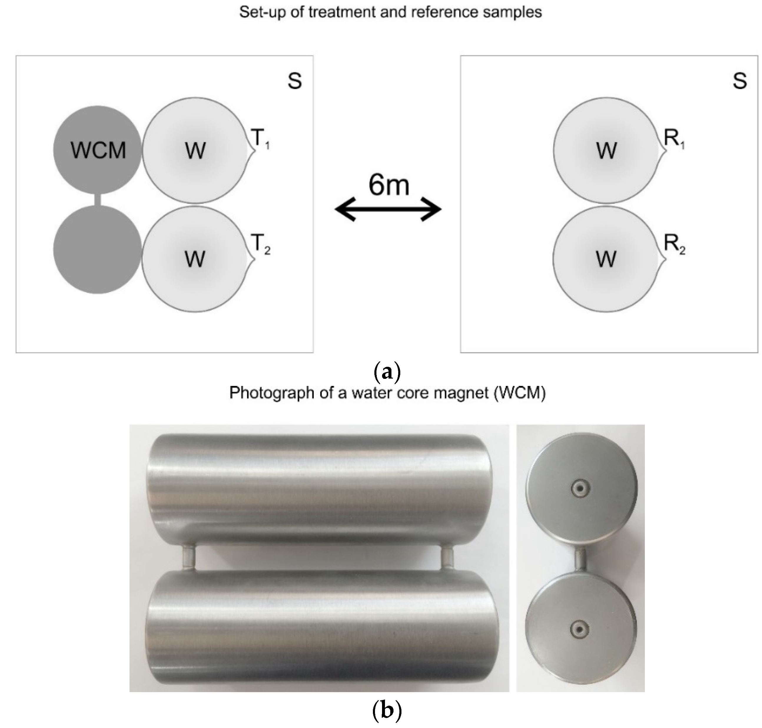
1.2. Water Core Magnets (WCMs)

Even before a reasonable theory on their mechanism was derived many companies had commercialized various types of magnetic water treatment devices [28,29]. WCMs, a type of commercially available devices, are employed to treat different kinds of water, like, e.g., potable tap water or water in cooling loops [30]. A WCM consists of two parallel stainless steel cylinders, welded together. Each cylinder is weakly magnetized and filled with water. The WCM is placed into the water to be treated. There is experimental evidence [2] that treatment devices can leak small amounts of iron from their casing changing the chemical and physical properties of the fluid to be treated and can thus influence scaling in a merely chemical way [31]. In order to avoid such leakage, we chose to expose our water samples to the WCM without contact to the device itself. Thus any effects measured would stem only from exposure to the magnetic field. The average absolute field strength of the WCMs used in this study is very weak, < 10 G at a distance of 5 mm from the surface, only one order of magnitude above the earth’s field and 2–3 orders of magnitude lower than that of a hard ferrite magnet [32]. However, its field contains a remarkable fine structure of strong gradients (~770~G·m⁻¹ (WCM 62081992) and 740~G·m⁻¹ (WCM 62083545), see results section). Such strong gradients are, as described above, a prerequisite for Coey’s theory. Therefore, WCMs provide an excellent basis for testing this theory.

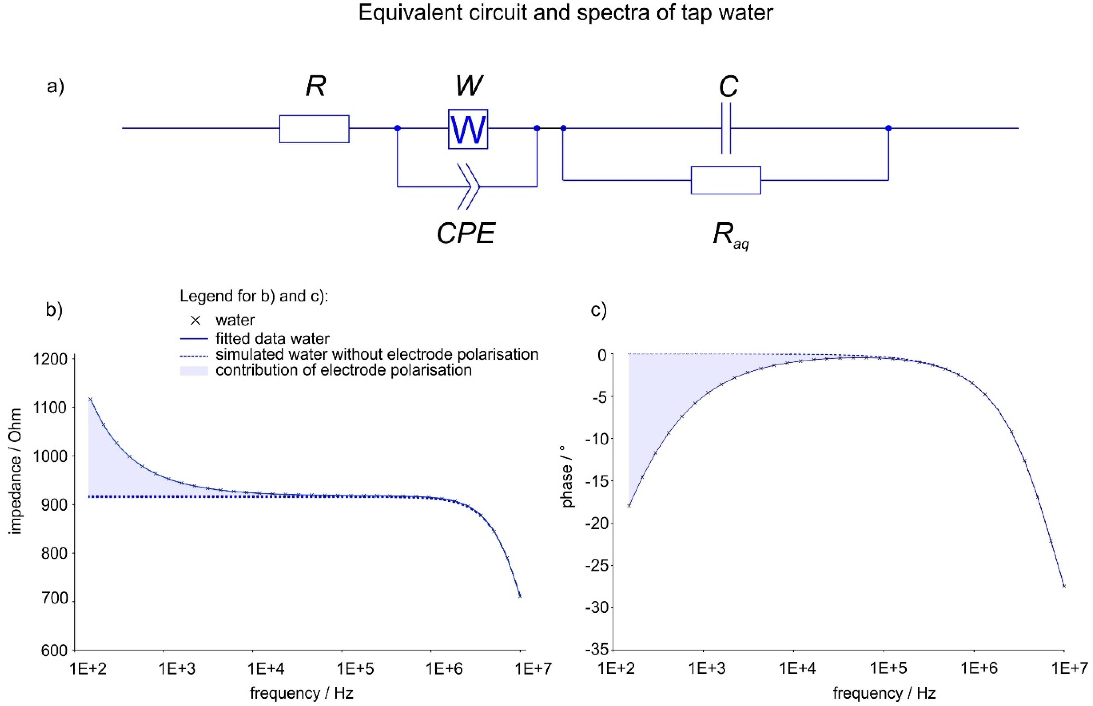
1.3. Electrical Impedance Spectroscopy (EIS)

EIS allows the depiction and simulation of a liquid as simple electric circuit. An aqueous solution behaves like a resistor and a capacitor in parallel: At frequencies below 10⁵–10⁶ Hz ions can move along with the field (resistive behaviour), and at frequencies above that, the dielectric properties of the solution begin to show (capacitive behaviour). At low frequencies (<10⁴ Hz), ions are fast enough to form layers at the electrodes, causing the so-called electrode polarisation (also referred to as Maxwell-Wagner polarisation). Mesoscale objects like DOLLOPs are much heavier than ions. They cannot follow the field as quickly and do not show the same polarisation behaviour. Electrode polarisation has no direct electric circuit equivalent, but can be simulated as a combination of certain elements [33]: A constant phase element (CPE) [34] with a Warburg impedance (W) in parallel to account for ion migration; R and W impedance represent bulk properties of the electrolyte solution and diffusion features of the probe in the solution [35]. The formation of DOLLOPs should thus be detectable by EIS in a threefold manner: the increase of R_aq due to the lower number of ions available, the decrease of the electrode polarisation for the same reason, and the inability of the (much heavier) DOLLOPs to follow the electric field and build layers, which should appear as a change of the CPE and W parameters, respectively. Figure 1 depicts the measured spectrum of a tap water sample (dots) and the calculated spectrum (line). The contribution of electrode polarisation is shown by simulating curves using the equivalent circuit (Figure 1a) without both Warburg impedance and CPE. These simulations are shown as dotted curves in Figure 1a,b. The contributions of the electrode polarisation are highlighted as blue areas.

1.4. Motivation for the Research Presented

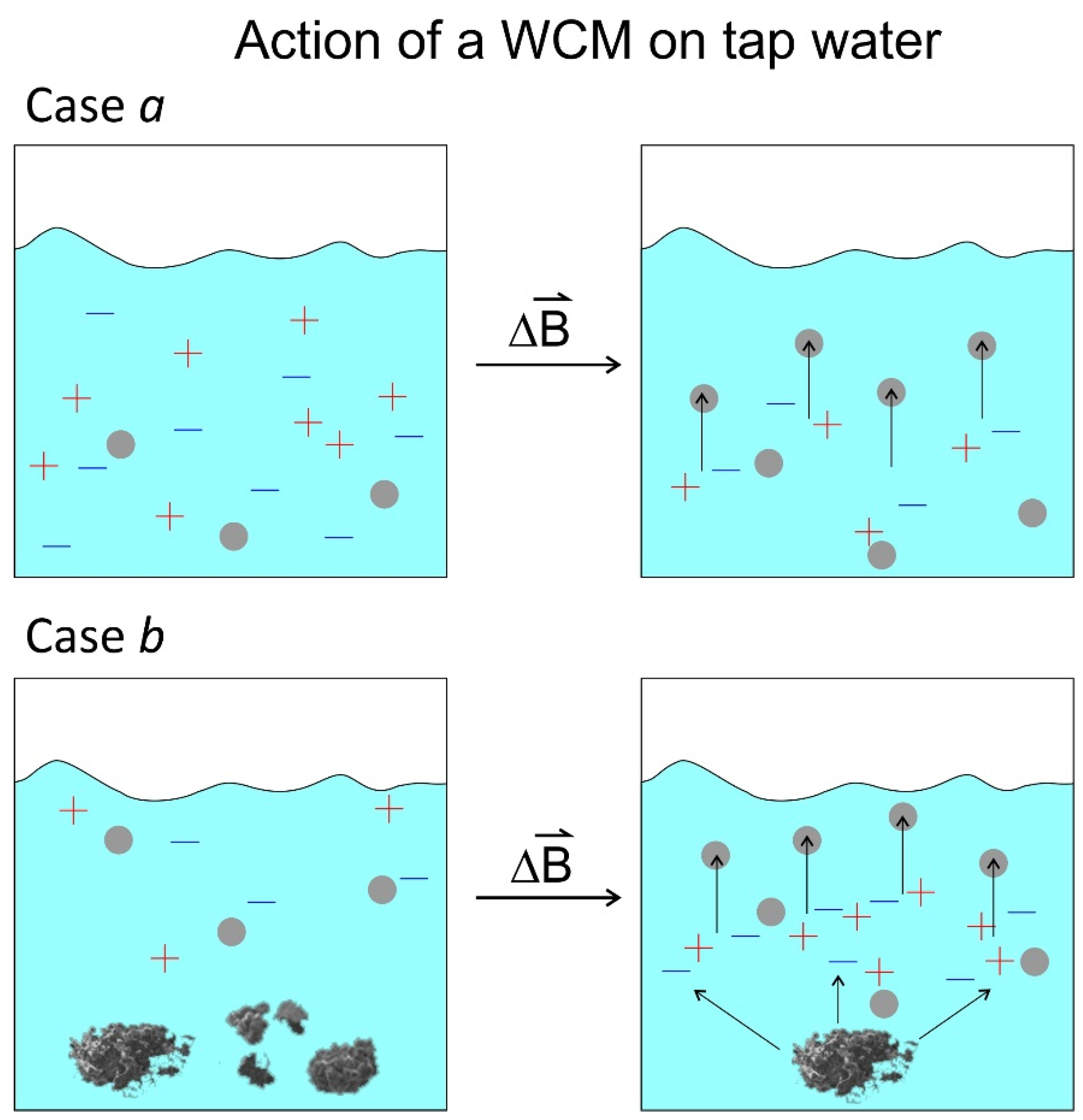
1.4.1. WCM as Treatment Device

Until recently the use of magnetic devices for water treatment or scale prevention was mostly considered charlatanry by a majority of the scientific community. The main argument was that explanatory models, which were based on the absolute field strength of the devices through the Lorentz force, failed to explain the observed effects fully or at least in part

$$F=q(E+v\times B)$$

(3)

The model of Coey [21], however, which is based upon the existence of the DOLLOPs and their agglomerations [27], entails that not absolute field strength but magnetic field gradients impact crystal growth dynamics. According to that theory very weak magnets can influence crystallisation as long as strong gradients are present. The WCMs investigated in this research fulfil this criterion: Their field is so weak (<10 G) that any appreciable Lorentz force action can be excluded, but it contains a fine structure of multiple strong local gradients as preamble for Coey’s theory.

1.4.2. Tap Water as Sample

The effectiveness of magnetic treatment devices on artificially prepared water solutions (defined calcium carbonate solutions) has been shown and discussed several times; the most recent investigations include (but are not limited to) the works of Higashintani, Coey, Kobe and Knez [4,13,15,16]. Their research provides the ground for this practically oriented work: Since in most industrial applications the water treated is tap water, [28,29,30] we deliberately chose tap water as sample. The ion content of our samples was analysed in five random samples taken over the time period of this investigation. The results of this study show that the ion content varied. However, even with this variability, general conclusions about the effectiveness of the treatment can be drawn, and crystallisation behaviour appears to be influenced according to Coey’s model.

2. Materials and Methods

2.1. Treatment Procedure

200 mL of tap water were filled into 250 mL beakers. To ensure proper sampling, beakers were filled after the tap water ran for 1 min. Two beakers were put next to the treatment devices (WCMs, type DZKL, IPF GmbH, Austria; see Figure 2a,b, two were placed in the same room at the same ambient conditions for at least 24 h and at most 7 days at two positions several meters apart in order to avoid inadvertent treatment of the reference sample.

At both locations the local magnetic field (without the presence of the treatment device) was lower than 0.5 G. Beakers and the water core magnets were put on plastic-covered, wooden (non-conducting and non-magnetic) surfaces. Treatment and reference position were randomly interchanged. Humidity and temperature were the same for both reference and treatment position (ambient conditions), since they were in the same laboratory at the same elevation. Two different treatment devices of the same type (water core magnet double cylinder) were used and exchanged randomly for different experiments. The beakers were covered with a watch glass to prevent dust and particulate contamination and to allow for continuous equilibration between the sample and atmosphere. After the treatment, at least three samples were taken from each beaker (two treated and two untreated beakers at least) resulting in a total of at least 12 individual measurements per experiment. All measurements were performed at room temperature. In order to check for the possibility of instrument drift of the impedance analyser, the sequential arrangement of measurements (treated and untreated) was changed in some experiments. The sequence of measurement had no influence on the results. As additional test for measurement reproducibility and sample location influence, several times test water samples were measured over days. These samples were placed at the same respective locations in the lab where the treatment and the reference samples were placed, but without the WCM near the treated sample. In these cases no significant differences between the samples of the two locations were found.

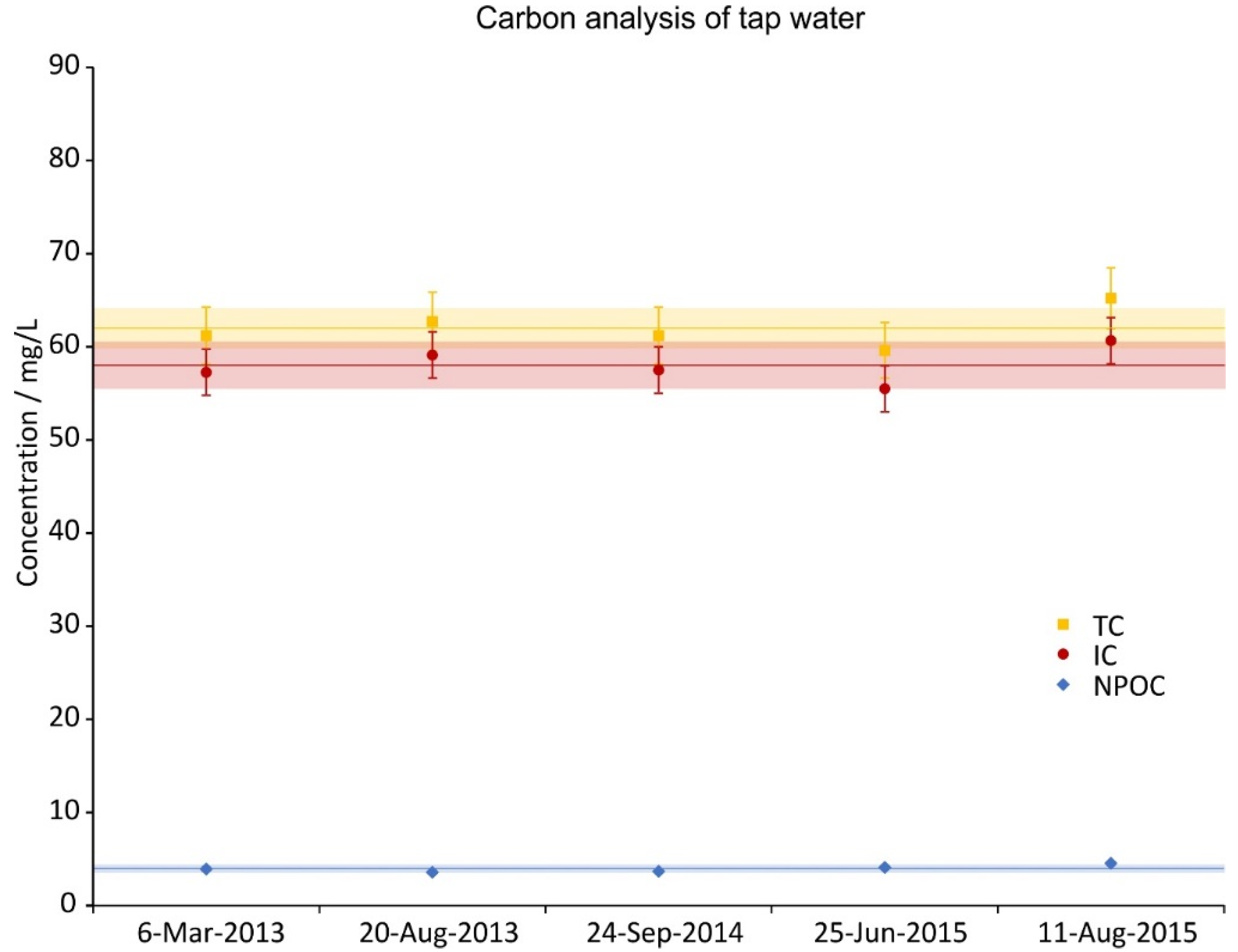
2.2. Tap Water Analysis

For the tap water analysis the following analytical instruments were used: A Perkin Elmer ICP type Optima 5300 DV with an ESI autosampler type SCA DX and a Polyscience water cooler type 6106P (PolyScience 6600 W. Touhy Avenue, Niles, Illinois 60714-4516 USA ). The software was Perkin Elmer WinLab32 version 4.0.2.0380; the internal standard solution was of 100 mg/L Y⁺³ and 2% nitric acid as rinse solution. The detection limit was 25–750 µg·L⁻¹ with an upper limit of 10,000 µg·L⁻¹. The total organic carbon (TOC) was measured with a Shimadzu TOC-L using a Shimadzu ASI-L autosampler and the standard software of that equipment. As reagents 2 M Hydrochloric acid and 25% Phosphoric acid were used. The detection limit was 1.00 mg·L⁻¹. For the IC anion analysis a Metrohm Compact IC Flex 930 ion chromatograph with a Metrohm Metrosep A Supp 5150/4.0 mm column was used. The pre-column was a Metrohm Metrosep A Supp 4/5 Guard. The conductivity detector, the CO₂ and the chemical suppressor are built into the ion chromatograph. A Spark Optimas auto sampler was used; the processing unit was a Metrohm, type MagIC Net. As reagents a mobile phase of 3.2 mM sodium carbonate and 1 mM sodium bicarbonate solution + 1% acetone was applied; the suppressor liquid was diluted phosphoric acid; the settings applied were a mobile phase flow of 0.7 mL·min⁻¹; Flow suppressor solutions 0.4 mL·min⁻¹; and runtime 20 min; the injection volume was 20 µL. The detection limit was 0.05–0.10 mg·L⁻¹ with an upper limit of 80 mg·L⁻¹ for Cl⁻ and 20 mg·L⁻¹ otherwise.

2.3. Impedance Analysis

All measurements were performed using an Impedance/Gain Phase Analyzer HP 4194A (Hewlett-Packard, CA, USA) which was connected via four BNC cables to a BDS 1200 connection head containing a BDS 1309 measurement cell (NOVOCONTROL Technologies, Montabaur, Germany). The BDS 1309 consists of two gold plated electrodes with a Teflon isolation ring in between, the diameter of the electrodes was 11 mm and the distance between the electrodes was 6.1 mm. This sample cell is especially designed for high permittivity liquids. A bipolar electrode configuration allowed measuring current separately while voltage was applied. The software WinDETA (NOVOCONTROL Technologies, Montabaur, Germany) was used to calibrate the system using the stray capacity of the cell (1.2 pF) and to perform the measurements. The complex impedance of the water samples were measured in a frequency range from 100 Hz to 10 MHz. In each spectrum 65 data points on a logarithmic scale from 100 Hz to 10 MHz were recorded with threefold internal averaging per point. Obtained impedance and phase spectra were fitted with “EIS Spectrum Analyser” software [36] using the Powell algorithm [37]. When treated and untreated water were compared, the electrode resistance (R) was determined in one fit and kept constant during the other.

2.4. SEM/EDX

SEM/EDX was performed with a JEOL JSM 6480 LV microscope (JEOL Technics Ltd., Tokyo, Japan) in high vacuum mode (emission electrons detection, acceleration voltage 10 kV, operating distance 10 mm).

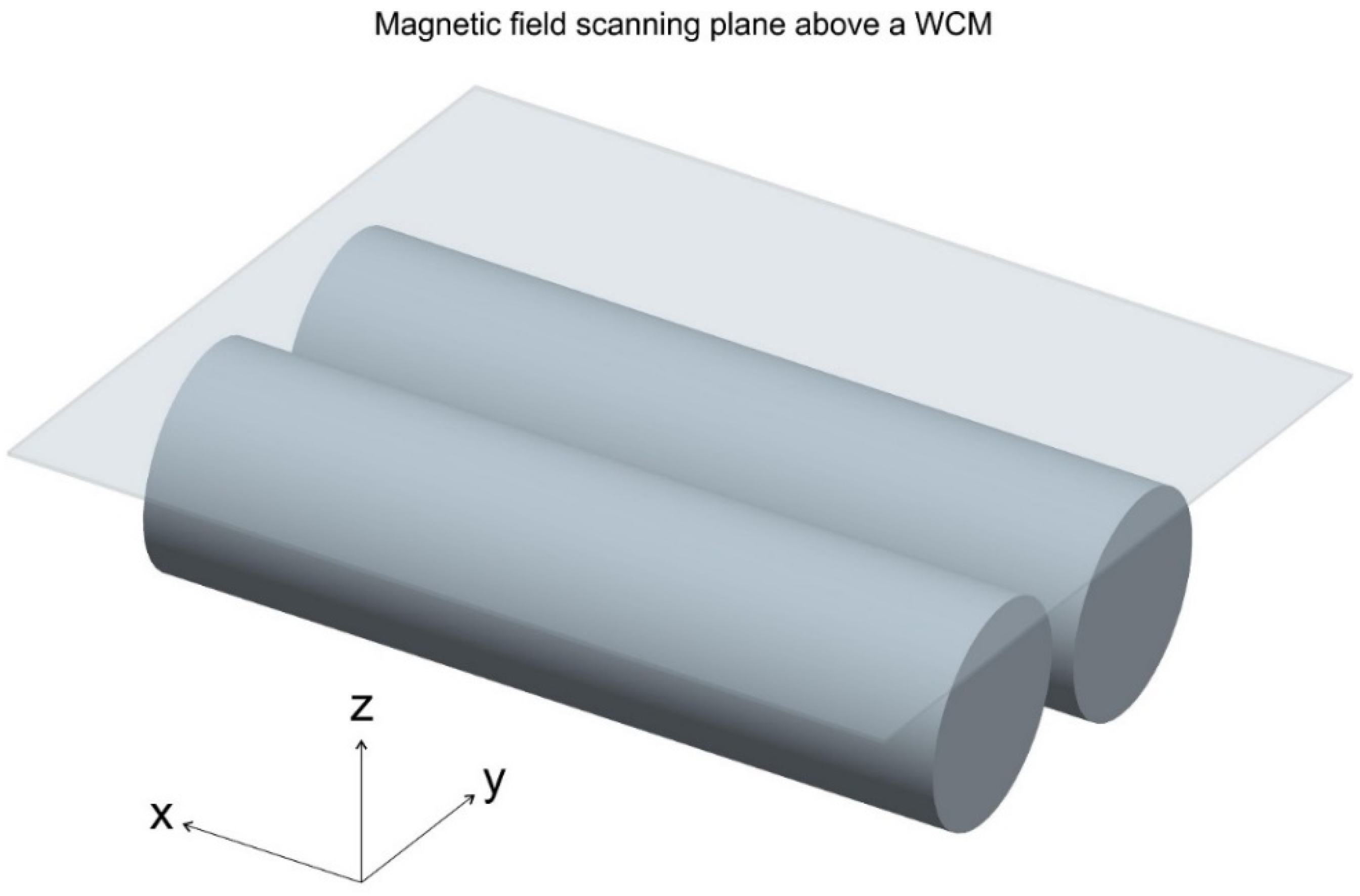
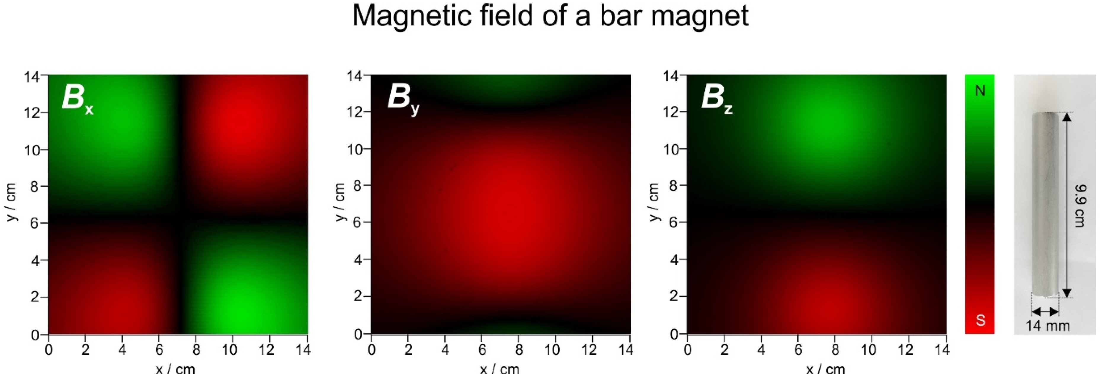
2.5. Magnetic Field Measurements and Visualisations

Magnetic fields of the WCMs were measured with a magnetometer (VGM, AlphaLab, Inc., Salt Lake City, UT, USA) mounted via a 30 cm long Plexiglas rod on a XYZ stage. This stage consisted of two Thorlabs LTS 300/M translation units for X and Y, and one LTS 150/M for the Z direction (Thorlabs GmbH, Dachau/Munich, Germany). The whole set-up was mounted on a TMC anti-vibration plate (75SSC-103-12 TMC Vibration control, TMC, 15 Centennial Drive, Peabody, MA, USA). The WCM to be scanned was put on a Plexiglas plate atop a wooden table. An area of 20 × 20 cm² was sampled with steps of 1 mm, 5 mm above the double cylinders (see Figure 3). Before each measurement, the sensor was zeroed inside a zero Gauss chamber (ZGC, AlphaLab Inc.) that reduces the environmental magnetic field (Earth field) to near zero (<0.002 G). Each point was repeatedly measured until all values (x, y and z direction of the magnetic field) would not differ more than 5% from each other in two subsequent measurements. The magnetic fields were then visualized by mapping the absolute values of the X, Y and Z components onto the RGB color space in each point. This procedure is described in detail with the example of a bar magnet in the results section.

2.6. Laser Scattering Measurements

For the laser scattering 22 samples of each analyte were measured using laser scattering in a microcapillary system (Guava easycyte 8HT, Merck Millipore, Merck KGaA, Darmstadt, Germany). Forward and sideward scatter of nm sized particles were detected in two dedicated photomultiplier tubes. Milli-Q water (deionized water, Millipore Corporation, resistivity 18 MΩ·cm) was run as blank. Data analyses was done using the InCyte software package of the system. Particle count data was retrieved plotting the forward scatter (logscale) and side scatter (logscale) data. Background noise was defined with the help of scattering data from Milli-Q water (blank value). The region was drawn into the plot leaving as little background data as possible in the actual counted area which was then used to retrieve the counts/sample.

2.7. Statistical Analysis

Statistical analyses have been performed using GenStat 17th Edition (VSN international Ltd., Hemel Hempstead, UK). For each experiment every frequency (n > 5) has been compared to blank values (n > 5) using a two sample two-sided t-test with a 95% confidence interval. The binominal test has been performed as a two-sided two sample test with a 95% confidence interval using normal approximation. Analyses of the data obtained have been performed using t-test. φ and Z of 65 single frequencies per experiment have been compared to blank values.

3. Results

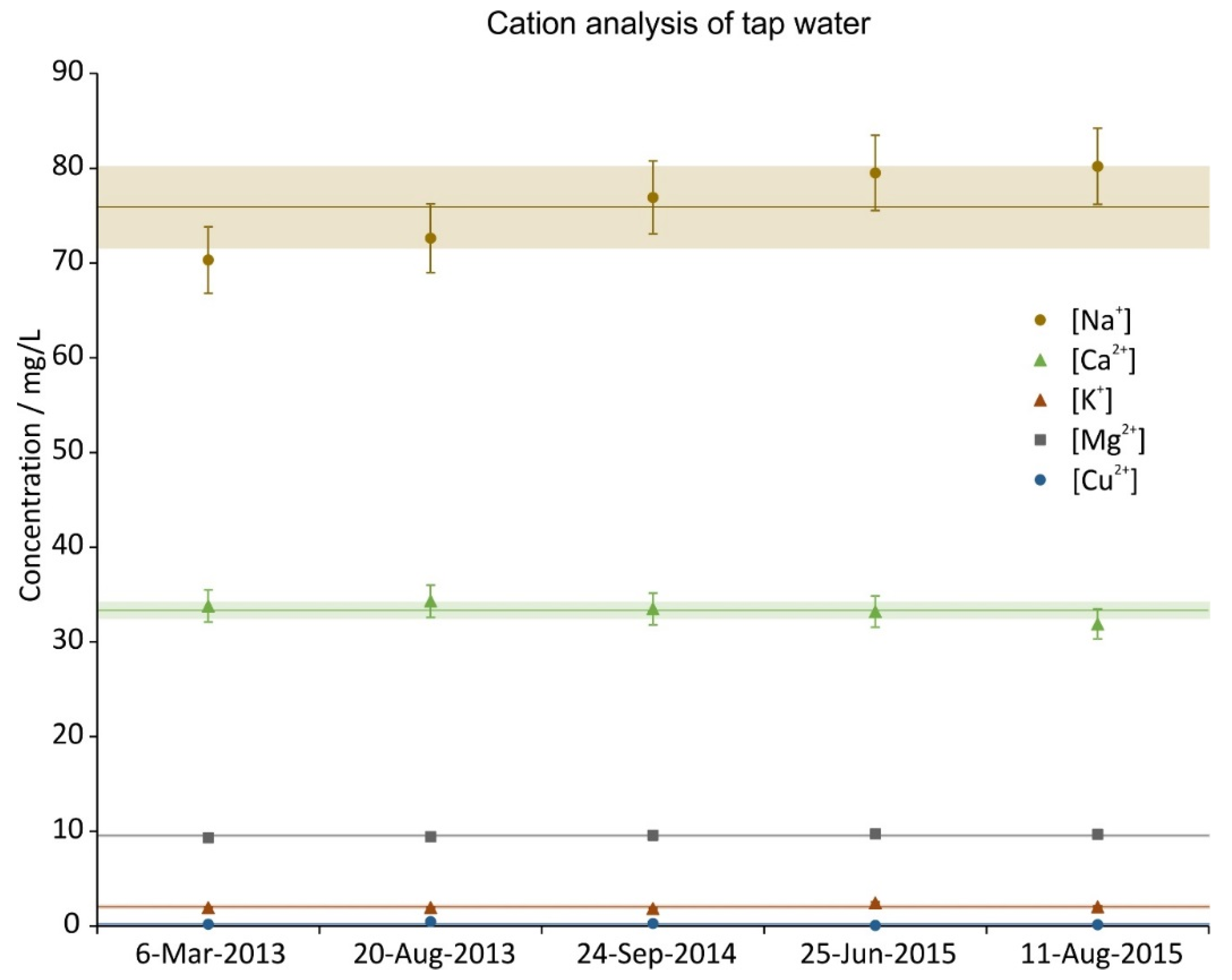
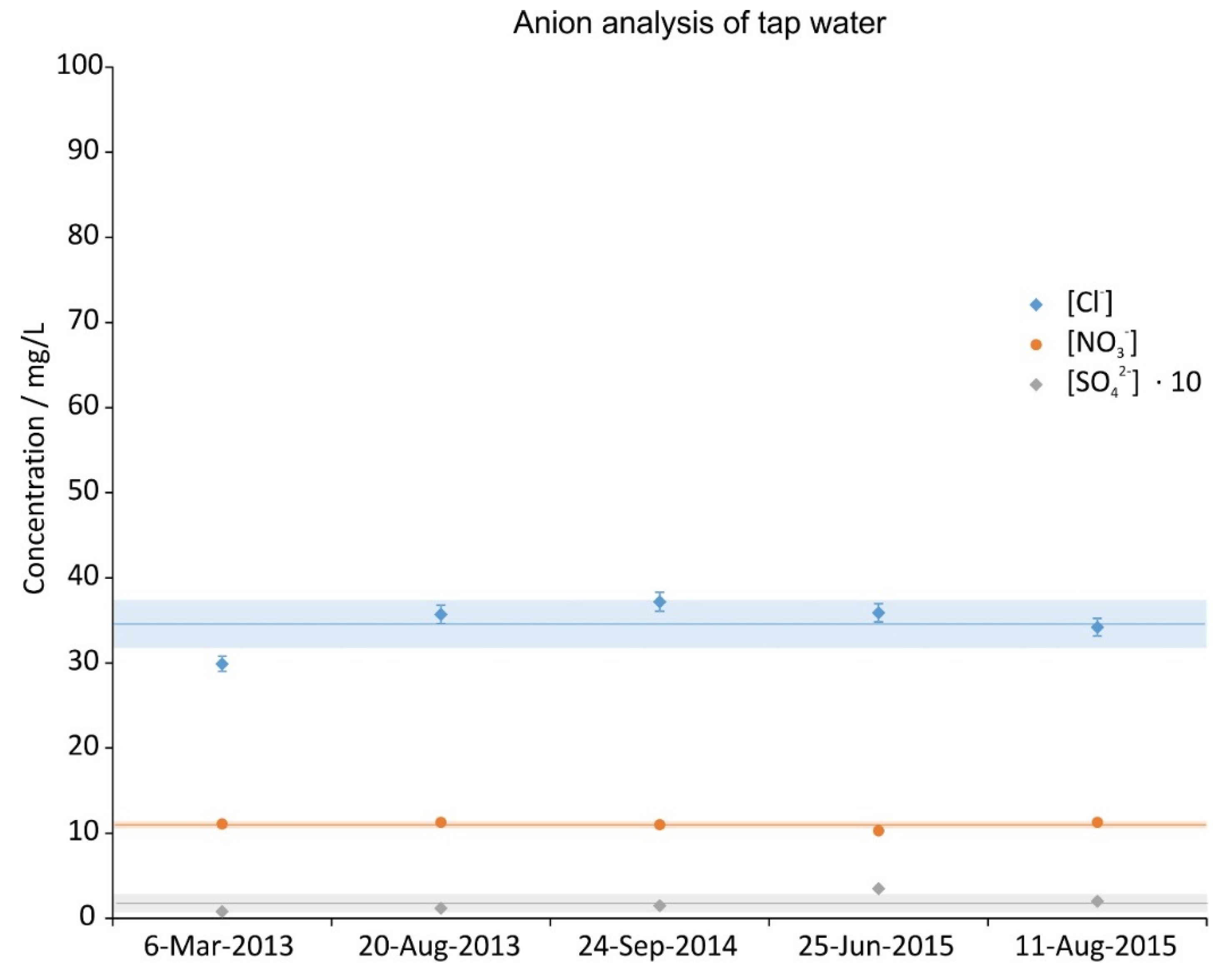
3.1. Tap Water Analysis

During the time period of the experiments five random tap water samples were taken and analysed. The concentration of their constituents is given in Figure 4, Figure 5 and Figure 6. The data was split in three graphs to increase their readability. In all graphs the same scale on the ordinate was chosen for reasons of comparison. Next to the ions shown, NO₂^-, PO₄³⁻, Fe^2+, Fe³⁺ were also investigated; their concentrations were below the LOQ (<0.05 mg/L). The analysis shows that the ion concentrations were fairly constant throughout the whole period (2.5 years).

Independent from this analysis, the tap water did sometimes contain minute amounts of visible precipitate which was probably from scaling in the pipes that broke free. Experiments both with and without such precipitates were carried out, the results are discussed in Section 3.4.

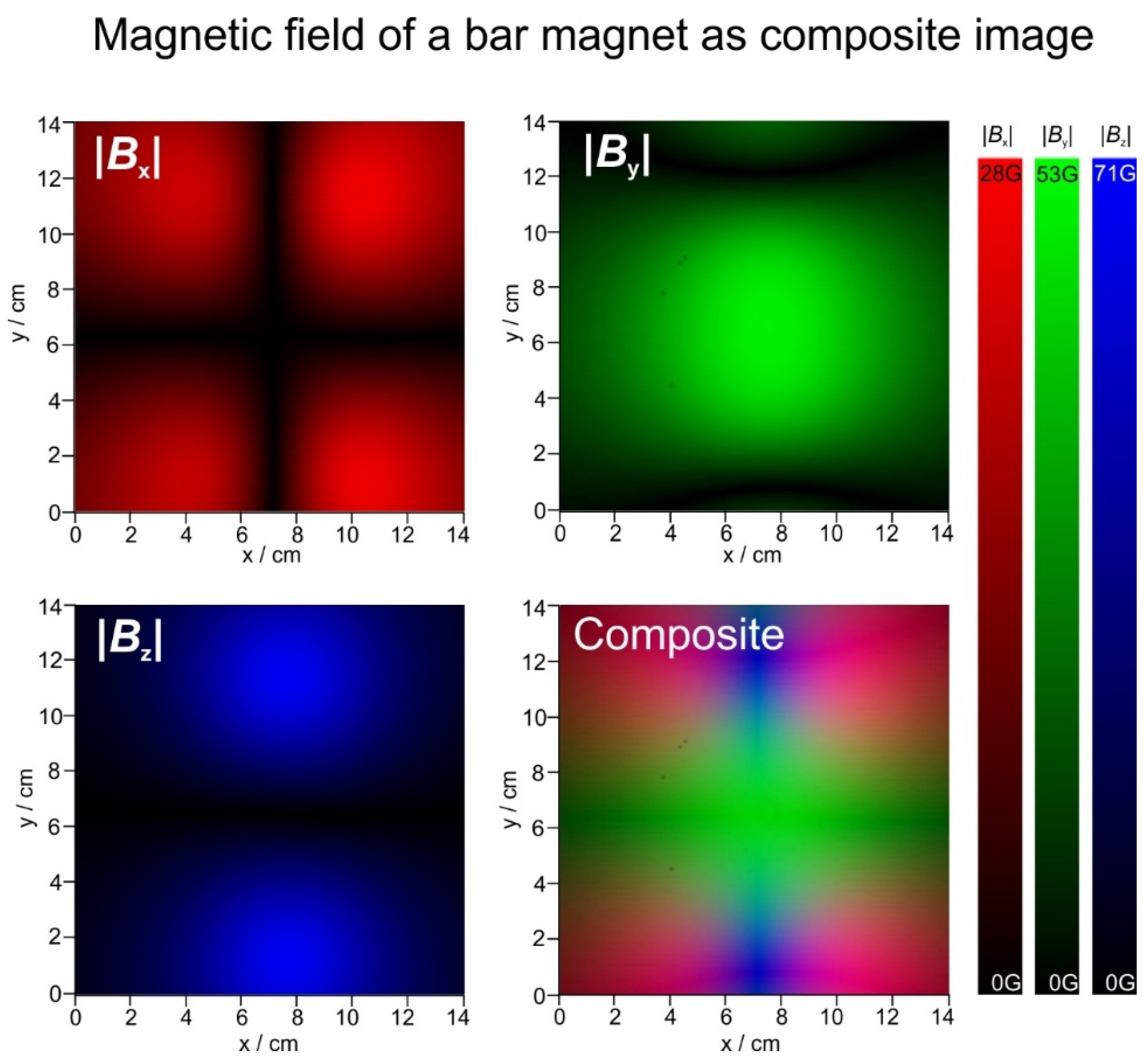
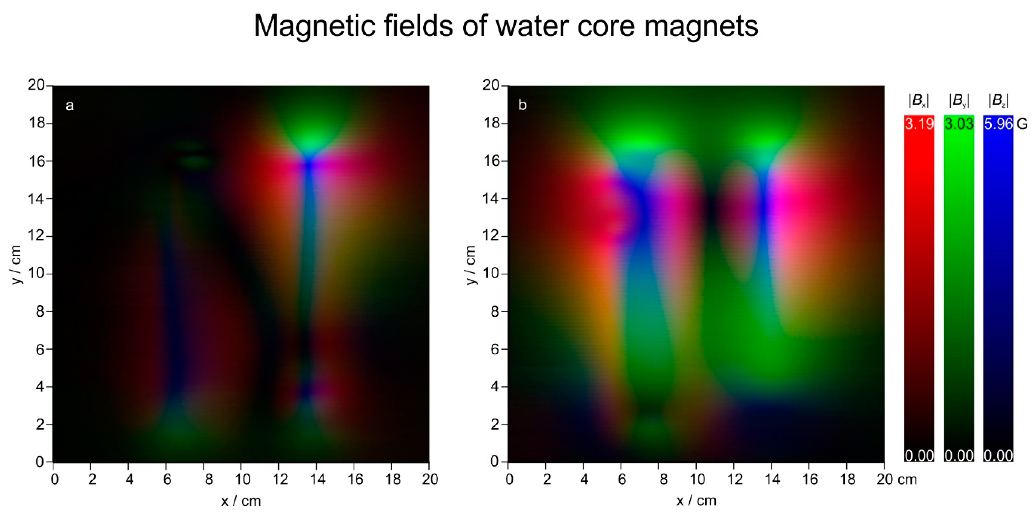
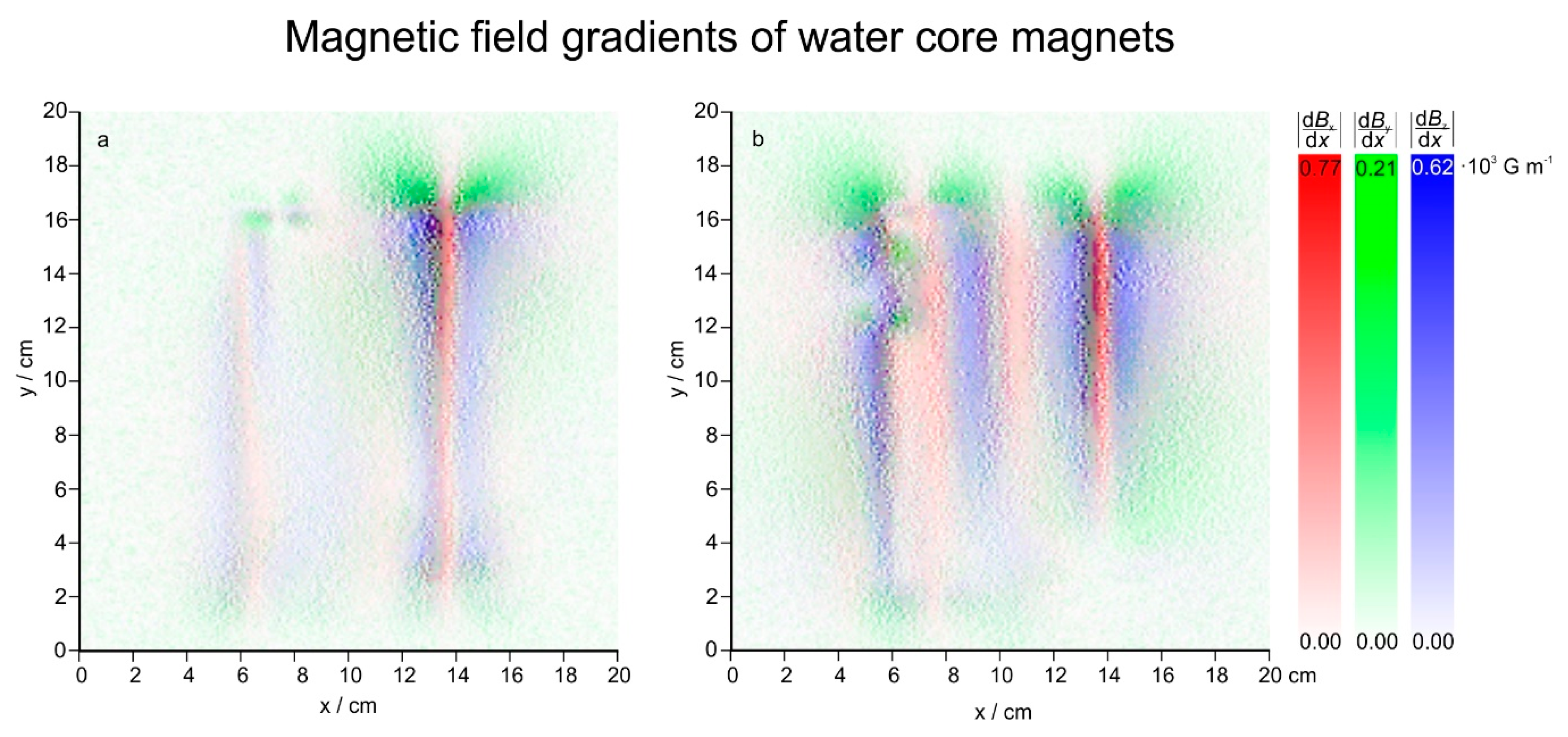
3.2. Magnetic Fields

In order to be able to read the magnetic field scan images properly, the analysis of a cylindrical bar magnet is presented first. Figure 7 shows the field of such a magnet scanned with the device described in the method section in an area of 14 × 14 cm², 3 cm above the magnet.

Because for the present analysis the sign (N or S) is not important, the field can also be displayed in terms of absolute intensity, and the three components can then be translated to the three primary colours, red (x), green (y) and blue (z). These images are then combined to a composite RGB image. This procedure is shown in Figure 8.

With the method describe above, composite images of magnetic fields of two different WCMs (serial numbers 62083545 and 62081992) are shown in Figure 9. The dark lines are sudden changes in magnetic field strengths resembling strong gradients. Gradients in x direction have been calculated and are shown in Figure 10. Here a scale from white to the primary colours is used in order to make a clear distinction from the composite images in Figure 9.

As can be seen from Figure 10, the magnetic field gradients of the WCMs are in the order of 770~G·m⁻¹ (WCM 62081992) and 740~G·m⁻¹ (WCM 62083545) or 0.077 T·m⁻¹ (WCM 62081992) and 0.074 T·m⁻¹ (WCM 62083545). Moreover, all gradients also seem to have a finer structure embedded. Because the 3-axis probe of the VGM magnetometer has its three sensors placed within less than 1.5 mm (according to the manual) of the probe’s end, a spatial resolution beyond that cannot be recorded. The presented gradients with a step size of 1 mm are probably already spatial averages, and the actual gradients present are probably even higher than 0.077 T·m⁻¹ (WCM 62081992) and 0.074 T·m⁻¹ (WCM 62083545). A higher gradient would not change the results of this investigation, nevertheless the authors plan to measure the field with a different system providing a higher resolution in the future.

As mentioned in the introduction, Coey [21] derived an inequality based on which the effectiveness of a magnetic device can be evaluated. For the sake of clarity and because of its importance, this inequality (2) is repeated here,

$$C=2\frac{L}{v}{f}_{p}a\nabla B\ge 1,$$

(4)

where C is the criterion, L the length of the magnetic device, v the velocity of the DOLLOPs, f_P the Larmor frequency of a proton, a the spin separation (0.25 nm) and ∇B the magnetic field gradient. If C ≥ 1, then the magnetic device can effectively influence the crystallisation of calcium carbonate. For the experiments presented, the magnetic device is larger than the volume of water treated, so the beaker diameter, 6 cm is used instead. One might argue at this point that for WCMs the actual width of the inhomogeneities, which is sometimes only a few mm, should be used, and not the measures of the device. Doing that does reduce C, but does not change the result (C ≥ 1, see end of this chapter) down to L values of 8 mm.

The velocity of the DOLLOPs can be calculated from the Brownian motion in a liquid using Fick’s law, $v=\frac{Dmg}{{\mathrm{k}}_{\mathrm{B}}T}$. In a dynamic equilibrium velocity is equal to the settling speed according to the Stokes-Einstein equation,

$$v=\frac{Dmg}{{\mathrm{k}}_{\mathrm{B}}T}=\mu mg=\frac{1}{\mathsf{\zeta }}mg=\frac{1}{6\pi \mathsf{\eta }r}mg$$

(5)

where D is the diffusion coefficient, k_B the Boltzmann constant, T the absolute temperature, µ and m are the mass and mobility of the DOLLOP, g is the acceleration due to gravity, ξ the drag coefficient, η the viscosity of the medium, and r the radius of a (assumingly) spherical DOLLOP. To know the mass of a 100 nm DOLLOP sphere, first its density must be calculated. Since a DOLLOP consists of both water (ρ_25°C = 1.00 g·cm⁻³) and aragonite (ρ = 2.93 g·cm⁻³), we assess its density as an equal mixture of both, so ρ_DOLLOP,25°C = 1.97 g·cm⁻³, resulting in a DOLLOP mass of 1.03 × 10⁻¹⁵ g. Taking water’s dynamic viscosity η_25°C = 0.89 × 10⁻⁴ Pa s, the resultant DOLLOP velocity due to Brownian motion is 0.012 mm·s⁻¹. The magnetic field gradients of the WCMs are in the order of 770~G·m⁻¹ (WCM 62081992) and 740~G·m⁻¹ (WCM 62083545) or 0.077 T·m⁻¹ (WCM 62081992) and 0.074 T·m⁻¹ (WCM 62083545) (see Figure 8), resulting in a Coey criterion of 0.077 T·m⁻¹ (WCM 62081992) and 0.074 T·m⁻¹ (WCM 62083545), thus clearly ≥ 1. The real gradients are probably higher as mentioned above, which would further increase the value of C and allow for higher fluid velocities. Smaller DOLLOPs than 100 nm are slower (the decrease of their mass in equal. 5 outweighs the increase of their mobility) and will therefore also further increase the value of C (velocity in Equation (4) is in the denominator).

The velocity of a DOLLOP also allows an estimation of the time required for the treatment to be effective. A straight travel from one side of the beaker to the other (6 cm) would take a 100 nm DOLLOP 1.4 h. During such a journey, a DOLLOP would encounter a number of magnetic field gradients. One should, however, also consider that Brownian motion is not unidirectional, the DOLLOP might be smaller and thus slower, and so the time should be multiplied by a factor of 10 or more in order to guarantee a successful treatment. This estimation matches with the observed time frames for a measureable treatment effect of about 24–48 h.

3.3. Evaporation

It has been shown [20] that magnetic fields can change the evaporation rate of electrolytic solutions. Within the measurement precision of our balances (1 mg) we did not see such an effect. It should be noted that a difference in evaporation was reported for field strengths much higher (~150 G) than applied in the present case (<10 G), which is why this observation is consistent with the proposed model and an additional confirmation of the stability of the atmospheric parameters.

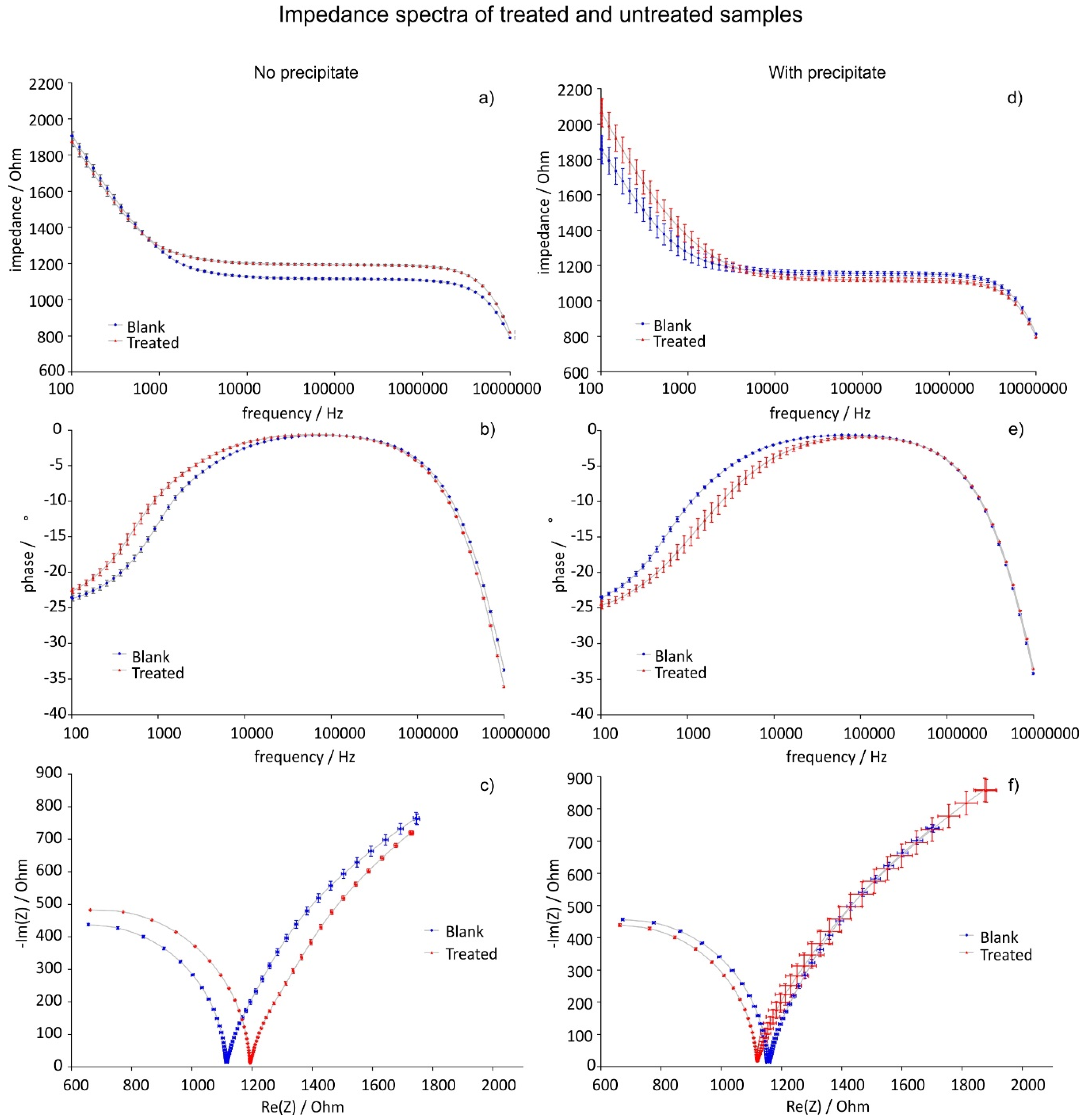
3.4. Complex Impedance

The proposed DOLLOP formation was tested in 16 independent experiments with at least 12 measurements per experiment, one measurement comprising the complex impedance at 65 frequencies, measuring two parameters (phase and impedance) per frequency. In each experiment at least two treated and two untreated samples were compared, and every sample was measured at least three times. t-test results for the treated samples compared to blank values showed statistically highly significant differences in 15 of 16 experiments (binominal exact probability < 0.001) either for phase (φ), for impedance (Z) or for both parameters. One experiment with 48 h treatment time did not show significant differences. In 9 of 16 experiments, Z showed frequency dependent variations which were highly different from the blank. In the case of differences a minimum of 4 and a maximum of 65 frequencies showed a significant difference, highly different results were obtained for 4 to 65 frequencies. In 15 of 16 experiments, φ showed frequency dependent variations which were highly different from the blank. Statistically significant differences in frequencies for a given φ occurred in a minimum of 2 and a maximum of 59 cases, highly significant results were calculated for 1 to 56 frequencies. In sum Z and φ showed statistically significant differences in a minimum of 3 and a maximum of 110 cases, highly different results in 2 to 106 frequencies. The exact binominal probability for an experiment to show a statistically highly different behaviour of treated water compared to untreated water is p < 0.001 (with 15 out of 16 cases positive for significant statistical values). These results are summarized in

Table 1. Statistics of the results of the WCM tapwater treatment. In each experiment, 65 frequencies between 100 Hz and 10 Mhz were scanned.

Parameter	Number
Number of experiments	16
Measurements per sample	≥3
Frequencies per measurement	65
Parameters per frequency	2
Significant difference (95% confidence interval)	15

.

Figure 11 shows exemplary impedance and phase changes of treated compared to untreated tap water. In addition to impedance (a,d) and phase (b,e), a Nyquist-plot of the data is shown (c,f). In this plot both the real and imaginary part of the impedance, |Z|·cos(φ) and -|Z|·sin(φ), are plotted against each other. On a Nyquist plot the impedance is a vector with characteristic length and angle, therefore a mandatory precondition is equal scales of the ordinate and abscissa axes. Such a scaling would, however, be unfavorable for the details of the spectra presented in this work, thus, we chose to omit this precondition in favor of a better representation of spectral details knowing well that the from such depictions the impedance can no longer be read out directly.Whereas a Nyquist plot does not give frequency information it is better in showing differences between spectra over the same frequency range since it combines both impedance and phase in one curve.

The curves depicted in Figure 11 were fitted using the model shown in Figure 1. The parameters of the circuit elements are given in

Table 2. Parameter fit for Figure 11, case a. The errors represent the quality of the fit for each element. $\mathrm{Blue}$ and $\mathrm{red}$ font colours are used to highlight an $\mathrm{increasing}$ or $\mathrm{decreasing}$ trend, respectively.

Parameter	Untreated		Treated		Absolute Difference	Relative Difference
R/Ω	238	±9	238	±6	0	0%
Aw/Ω·s−0.5	22,593	±11	21,202	±511	−1391	−6%
CPE P × 107	2.01	±0.32	4.37	±0.37	2.36	+118%
CPE n	1.00	±0.02	0.97	±0.01	−0.031	−3%
C/pF	17.7	±0.98	16.8	±1.4	−0.989	−6%
Raq/Ω	870	±9	951	±8	81	+9%

(case a) and

Table 3. Parameter fit for Figure 11, case b. The errors represent the quality of the fit for each element. $\mathrm{Blue}$ and $\mathrm{red}$ font colours are used to highlight an $\mathrm{increasing}$ or $\mathrm{decreasing}$ trend, respectively.

Parameter	Untreated		Treated		Absolute Difference	Relative Difference
R/Ω	232	±7	232	±10	0	0%
Aw/Ω·s−0.5	21,721	±10	24,967	±1064	3246	+15%
CPE P · 107	3.63	±0.34	1.10	±0.25	−2.53	−70%
CPE n	0.98	±0.01	1.00	±0.03	0.019	+2%
C/pF	16.9	±0.65	17.3	±1.1	0.342	+2%
Raq/Ω	917	±7	877	±11	−40	−4%

(case b), respectively. Next to that, average curves of all 16 measurements were fitted with this model. Although sample composition and treatment time were not identical for all experiments as described in the experimental section, the most important model parameter, the conductivity of the water (R_aq), shifted consistently depending on the case (a or b). This result is shown in

Table 4. Case dependent average of tap water resistance parameter R_aq fitted according to the model presented in Figure 1, including standard error. The quality of the fits can be appreciated from the average fitting error of this parameter, E_{Raq, av} and its associated standard error.

Case	Δ Raq, av /Ω	ERaq, av /Ω
a (8 experiments)	31 ± 9	14 ± 3
b (8 experiments)	−39 ± 9	13 ± 2

.

The direction in which this change was observed depended on the constituents of the original tap water:

• Case a: No precipitation

When no micro precipitation was present in the beakers before and after the treatment, the impedance of the treated sample increased at high frequencies (case a, see Figure 11a–c, increase of R_aq in Table 2). Because fewer ions are available in the solution due to DOLLOP formation, there is less electrode polarisation at low frequencies (smaller phase shift in Figure 7b at low frequencies and decrease of A_w (ion diffusion constant) and C in Table 2).

As mentioned in Section 3.1 sometimes the initial tap water contained tiny crystals. In some cases, precipitation would form during the treatment time in the reference beaker. Both of these cases are summarized in this work as case b:

• Case b: precipitation

If there was visible micro precipitate in the reference beakers after the treatment or both beakers before treatment, the impedance of the treated sample was lower at high frequencies than the reference meaning that there were more ions in solution (case b, see Figure 11d–f, decrease of R_aq in Table 3), and higher at low frequencies due to increased electrode polarisation caused by these ions (larger phase shift in Figure 11e at low frequencies and increase of A_w and C in Table 2). Also here DOLLOPs are formed as described in case a, but the solubility product allows additional ions to dissolve from the precipitate. The solution is thus in a dynamic equilibrium between the formation of DOLLOPs and the solvation of the µm sized particles (see Figure 12). The impedance increase observed suggests that the magnetic field gradient does not only facilitate the formation of DOLLOPs but also the dissolution of micro crystals. The authors plan to investigate this hypothesis in subsequent work.

In no case was precipitation found in the treated beaker after treatment, corroborating the DOLLOP formation hypothesis. In general, the shift in case b was smaller than in case a; and in the one case where we did not see a significant effect of the treatment, a trend towards case b was observable.

Next to ion diffusion constant, capacity and resistivity; parameters of the constant phase element (CPE) show large differences between the fits of the spectra from treated and untreated samples, again in opposite direction for cases a and b like the other parameters. The physical meaning of a CPE is an ongoing discussion in general; however, for the purpose of this work it is sufficient to say that, according to the model, together with the Warburg impedance it represents electrode polarisation and ion migration. Differences in the mobility of the ionic content of the solution due to the DOLLOP formation are also reflected in different parameters of the CPE.

A simplified sketch of this mechanism is given in Figure 12.

These findings are in line with the many observations reported in theliterature [4,6,13,15,16,38,39,40] and most importantly, they agree with the model of Coey [21]: the strong local gradients act on the mechanism of precipitation and induce DOLLOP formation. In case a, the ions form many small nuclei, DOLLOPs, which form a colloid and are thus no longer able to follow the alternating electric field during the impedance measurement.

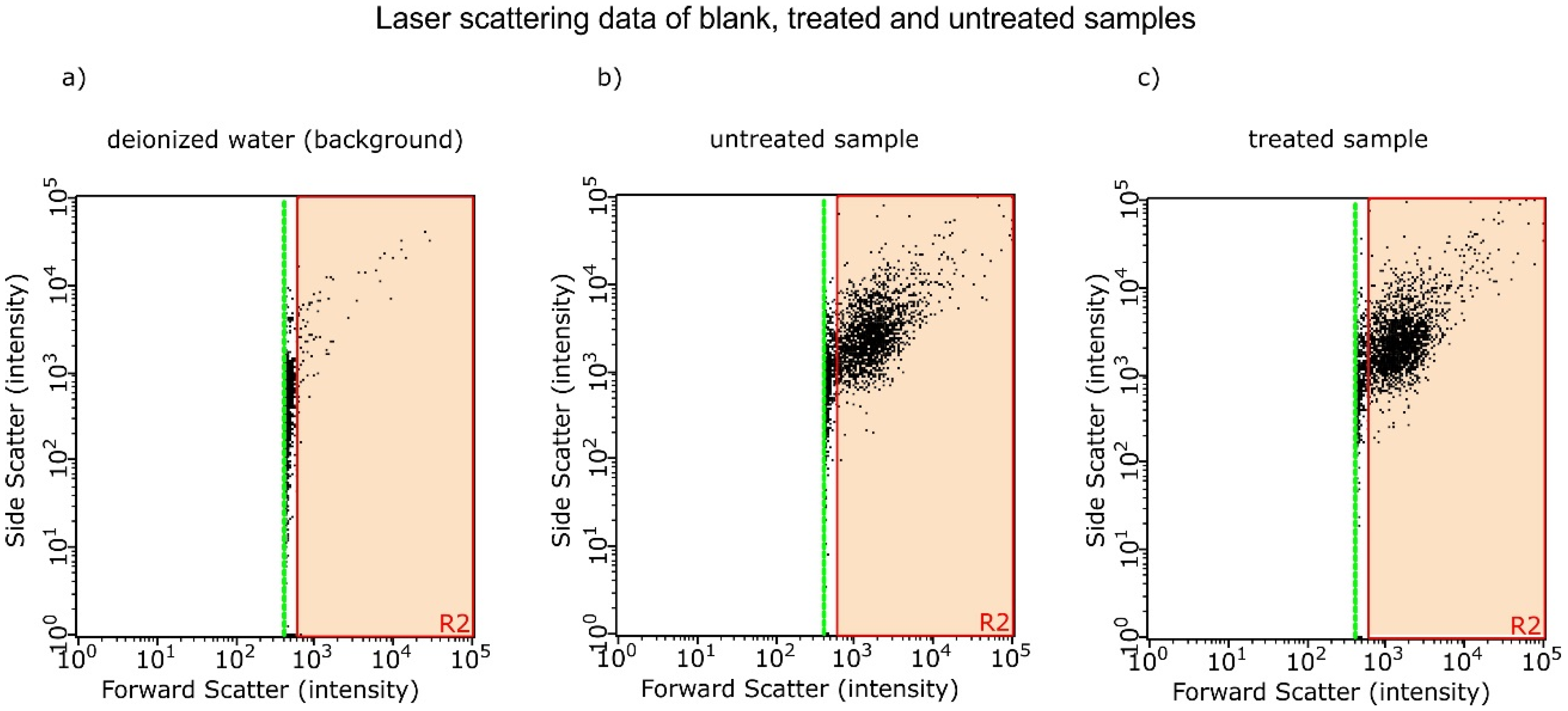
3.5. Laser Scattering

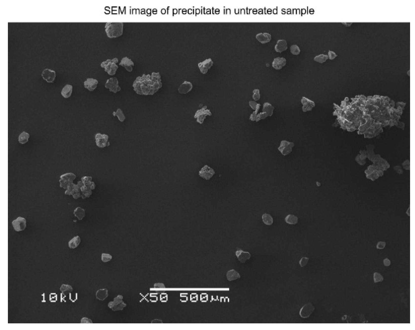
Since these DOLLOPs are much smaller than 1 µm, their colloid is invisible to the naked eye due to the small cross-sections for Rayleigh scattering. Next to the EIS measurement, we were able to confirm their presence by investigating samples from two experiments with laser scattering. We compared 22 treated to 22 untreated samples in each experiment and found a significant increase up to 25% of nm sized objects in the treated sample (p < 0.001) compared to the reference. Figure 13 shows exemplary scattering plots for deionized water (milli-Q water, background), treated and untreated sample;

Table 5. Number of objects determined by laser scattering in two treated and untreated solutions from 22 samples each.

Experiment	Untreated/104 Counts mL−1	Treated/104 Counts mL−1	Difference Treated vs. Untreated
Experiment 1	2.72 ± 0.02	3.01 ± 0.04	P < 0.001
Experiment 2	5.17 ± 0.02	7.00 ± 0.10	P < 0.001

summarizes the results of these experiments.

3.6. SEM/EDX

Precipitate was collected from the reference beaker with a spatula and investigated using SEM/EDX. The analysis revealed it to be mainly oxygen, calcium and carbon. Their ratios suggest hydrogen carbonate and possibly the presence of organic material. A representative image of the precipitate from the untreated sample is shown in Figure 14; a representative EDX analysis is given in

Table 6. EDX analysis of the precipitate shown in Figure 10.

Element, Line	Weight %	Atom %
Carbon, K	13.23	18.87
Oxygen, K	68.28	73.11
Magnesium, K	0.40	0.28
Phosphorus, K	0.00	0.00
Sulfur, K	0.01	0.01
Potassium, K	0.06	0.02
Calcium, K	18.03	7.71
Iron, L	0.00	0.00
Total	100.00	100.00

.

4. Conclusions

According to a theory derived by Coey [21], crystallisation of calcium carbonate can be influenced by strong magnetic field gradients independent of the absolute field strength of the magnet. We tested this theory by exposing tap water samples to so-called water core magnets (WCMs). The absolute fields of WCMs are weak (<10 G). However, these fields display a fine pattern of strong field gradients (≤770~G·m⁻¹ (WCM 62081992) and 740~G·m⁻¹ (WCM 62083545)). By electrical impedance spectroscopy (EIS) and laser scattering we measured significant differences in crystallisation behaviour of exposed tap water samples. The results can be interpreted as an enhanced formation of DOLLOPs, mesoscale prenucleation clusters, due to exposure to a WCM field. We have thus shown that, as Coey’s inequality predicts, magnetic treatment with very weak fields can be effective as long as strong gradients are present in the field.

References

1. Josh, K.M.; Kamat, P.V. Effect of magnetic field on the physical properties of water. J. Ind. Chem. Soc. 1966, 43, 620–622. [Google Scholar]
2. Duffy, E.A. Investigation of Magnetic Water Treatment Devices. Ph.D. Thesis, Clemson University, Clemson, SC, USA, 1977. [Google Scholar]
3. Lin, I.; Yotvat, J. Exposure of irrigation and drinking water to a magnetic field with controlled power and direction. J. Mag. Magn. Mat. 1990, 83, 525–526. [Google Scholar] [CrossRef]
4. Higashitani, K.; Kage, A.; Katumura, S.; Imai, K.; Hatade, S. Effects of a magnetic field on the formation of CaCO3 particles. J. Colloid Interface Sci. 1993, 156, 90–95. [Google Scholar] [CrossRef]
5. Gehr, R.; Zhai, Z.A.; Finch, J.A.; Rao, S.R. Reduction of soluble mineral concentrations in CaSO4 saturated water using a magnetic field. Water Res. 1995, 29, 933–940. [Google Scholar] [CrossRef]
6. Baker, J.S.; Judd, S.J. Magnetic amelioration of scale formation. Water Res. 1996, 30, 247–260. [Google Scholar] [CrossRef]
7. Pach, L.; Duncan, S.; Roy, R.; Komarneni, S. Effects of a magnetic field on the precipitation of calcium carbonate. J. Mater. Sci. Lett. 1996, 15, 613–615. [Google Scholar] [CrossRef]
8. Wang, Y.; Babchin, A.J.; Chernyi, L.T.; Chow, R.S.; Sawatzky, R.P. Rapid onset of calcium carbonate crystallization under the influence of a magnetic field. Water Res. 1997, 31, 346–350. [Google Scholar] [CrossRef]
9. Parsons, S.A.; Wang, B.L.; Judd, S.J.; Stephenson, T. Magnetic treatment of calcium carbonate scale-effect of pH control. Water Res. 1997, 31, 339–342. [Google Scholar] [CrossRef]
10. Barrett, R.A.; Parsons, S.A. The influence of magnetic fields on calcium carbonate precipitation. Water Res. 1998, 32, 609–612. [Google Scholar] [CrossRef]
11. Colic, M.; Morse, D. The elusive mechanism of the magnetic 'memory'of water. Colloid Surface A 1999, 154, 167–174. [Google Scholar] [CrossRef]
12. Goldsworthy, A.; Whitney, H.; Morris, E. Biological effects of physically conditioned water. Water Res. 1999, 33, 1618–1626. [Google Scholar] [CrossRef]
13. Coey, J.M.D.; Cass, S. Magnetic water treatment. J. Magn. Magn. Mater. 2000, 209, 71–74. [Google Scholar] [CrossRef]
14. Hołysz, L.; Chibowski, E.; Szcześ, A. Influence of impurity ions and magnetic field on the properties of freshly precipitated calcium carbonate. Water. Res. 2003, 37, 3351–3360. [Google Scholar] [CrossRef]
15. Kobe, S.; Dražić, G.; McGuiness, P.J.; Meden, T.; Sarantopolou, E.; Kollia, Z.; Sefalas, A.C. Control over nanocrystalization in turbulent flow in the presence of magnetic fields. Mater. Sci. Eng. 2003, 23, 811–815. [Google Scholar] [CrossRef]
16. Knez, S.; Pohar, C. The magnetic field influence on the polymorph composition of CaCO3 precipitated from carbonized aqueous solutions. J. Colloid Interface Sci. 2005, 281, 377–388. [Google Scholar] [CrossRef] [PubMed]
17. Fathia, A.; Mohamed, T.; Claude, G.; Maurin, G.; Mohamed, B.A. Effect of a magnetic water treatment on homogeneous and heterogeneous precipitation of calcium carbonate. Water Res. 2006, 40, 1941–1950. [Google Scholar] [CrossRef] [PubMed]
18. Li, J.; Liu, J.; Yang, T.; Xiao, C. Quantitative study of the effect of electromagnetic field on scale deposition on nanofiltration membranes via UTDR. Water Res. 2007, 41, 4595–4610. [Google Scholar] [CrossRef] [PubMed]
19. Katsir, Y.; Miller, L.; Aharanov, Y.; Jacob, E.B. The effect of rf-irradiation on electrochemical deposition and its stabilization by nanoparticle doping. J. Electrochem. Soc. 2007, 154, 249–259. [Google Scholar] [CrossRef]
20. Hołysz, L.; Szcześ, A.; Chibowski, E. Effects of a static magnetic field on water and electrolyte solutions. J. Colloid Interface Sci. 2007, 316, 996–1002. [Google Scholar] [CrossRef] [PubMed]
21. Coey, J.M.D. Magnetic water treatment-how might it work? Phil. Mag. 2012, 92, 3857–3865. [Google Scholar] [CrossRef]
22. Gebauer, D.; Völkel, A.; Cölfen, H. Stable prenucleation calcium carbonate clusters. Science 2008, 322, 1819. [Google Scholar] [CrossRef] [PubMed]
23. Pouget, E.M.; Bomans, P.H.H.; Goos, J.A.C.M.; Frederik, P.M.; de With, G.; Sommerdijk, N.A.J.M. The Initial Stages of Template-Controlled CaCO3 Formation Revealed by Cryo-TEM. Science 2009, 323, 1455–1458. [Google Scholar] [CrossRef] [PubMed] [Green Version]
24. Raiteri, P.; Gale, J.D. Water is the key to nonclassical nucleation of amorphous calcium carbonate. J. Am. Chem. Soc. 2010, 132, 17623–17634. [Google Scholar] [CrossRef] [PubMed]
25. Gebauer, D.; Cölfen, H. Prenucleation clusters and non-classical nucleation. Nano Today 2011, 6, 564–584. [Google Scholar] [CrossRef]
26. Wolf, S.E.; Müller, L.; Barrea, R.; Kampf, C.J.; Leiterer, J.; Panne, U.; Hoffmann, T.; Emmerling, F.; Tremel, W. Carbonate-coordinated metal complexes precede the formation of liquid amorphous mineral emulsions of divalent metal carbonates. Nanoscale 2011, 3, 1158–1165. [Google Scholar] [CrossRef] [PubMed]
27. Demichelis, R.; Raiteri, P.; Quigley, J.D.; Gebauer, D. Stable prenucleation mineral clusters are liquid-like ionic polymers. Nat. Commun. 2011, 2, 590. [Google Scholar] [CrossRef] [PubMed]
28. Donaldson, J.D. Magnetic treatment of fluids-preventing scale. Finish 1988, 12, 22–32. [Google Scholar]
29. Spear, M. The growing attraction of magnetic treatment. Process. Eng. 1992, 73, 143. [Google Scholar]
30. Zunkovič, K. Wasserbelebung am Beispiel Grander-Technologie: Eine Empirische Erhebung unter industriellen Anwendern. Diploma Thesis, University of Graz, Graz, Austria, 2007. [Google Scholar]
31. Busch, K.W.; Busch, M.A.; Parker, D.H.; Darling, R.E.; McAtee, J.L., Jr. Studies of a water treatment device that uses magnetic fields. Corrosion 1986, 42, 211–221. [Google Scholar] [CrossRef]
32. Goldman, A. Modern Ferrite Technology; Springer: New York, NY, USA, 2006. [Google Scholar]
33. Sammer, M.; Laarhoven, B.; Mejias, E.; Yntema, D.; Fuchs, E.C.; Holler, G.; Brasseur, G.; Lankmayr, E. Biomass measurement of living Lumbriculus variegatus with impedance spectroscopy. J. Electrical Bioimpedance 2014, 5, 92–98. [Google Scholar] [CrossRef]
34. Brug, G.; van den Eeden, A.L.G.; Sluyters-Rehbach, M.; Sluyters, J.H. The analysis of electrode impedances complicated by the presence of a constant phase element. J. Electroanal. Chem. Interfacial Electrochem. 1984, 176, 275–295. [Google Scholar] [CrossRef]
35. Santos, M.B.D.; Agusil, J.P.; Prieto-Simón, B.; Sporer, C.; Teixeira, V.; Samitier, J. Highly sensitive detection of pathogen Escherichia coli O157: H7 by electrochemical impedance spectroscopy. Biosens. Bioelectron. 2013, 45, 174–180. [Google Scholar] [CrossRef] [PubMed]
36. Bondarenko, A.S.; Ragoisha, G.A. Inverse Problem in Potentiodynamic Electrochemical Impedance. In Progress in Chemometrics Research; Pomerantsev, A.L., Ed.; Nova Science Publishers: New York, NY, USA, 2005; pp. 89–102. [Google Scholar]
37. Powell, M. An efficient method for finding the minimum of a function of several variables without calculating derivatives. Comput. J. 1964, 7, 155–162. [Google Scholar] [CrossRef]
38. Martynova, O.I.; Tebenekhin, E.F.; Gusev, B.T. Conditions and mechanism of deposition of the solid calcium carbonate phase from aqueous solutions under the influence of a magnetic field. Colloid J. USSR 1967, 29, 512–514. [Google Scholar]
39. Chechel, P.S.; Annenkova, G.V. Influence of magnetic treatment on solubility of calcium sulphate. Coke Chem. R 1972, 8, 60–61. [Google Scholar]
40. Kronenberg, K.J. Experimental evidence for effects of magnetic fields on moving water. IEEE Trans. Magn. 1985, 21, 2059–2061. [Google Scholar] [CrossRef]
Figure 1. (a) Equivalent circuit; (b) exemplary impedance Z; (c) phase spectra (φ, subfigure c) of tap water incl. fitting results. R, W and CPE are resistance, Warburg impedance and constant phase element simulating electrode polarization and ion migration; C and Raq the capacitance and resistance of tap water.
Water 08 00079 g001
Figure 2. (a) Sketch showing the set-up for the treatment and the reference; S: plastic base (table), WCM: water core magnet, W: watch glass covering the beakers, T: treated beakers, R: reference beakers. (b) Water core magnet treatment device type DZKL (cylinder radius 2.25 cm, height 15 cm, distance between cylinders 1 cm).
Water 08 00079 g002
Figure 3. Sketch showing the area (20 × 20 cm2) scanned for the magnetic field measurements with the water core magnet underneath (two cylinders, 18 cm length, 5 cm diameter, 1 cm apart).
Water 08 00079 g003
Figure 4. Cation concentration of 5 random tap water samples during the investigation period. The error bars show the precision of the measurement (5%), the lines are the averages and the shaded regions depict the standard deviations over the 5 samples.
Water 08 00079 g004
Figure 5. Anion concentration of 5 random tap water samples during the investigation period. The error bars show the precision of the measurement (3%), the lines are the averages and the shaded regions depict the standard deviations over the 5 samples.
Water 08 00079 g005
Figure 6. Total carbon (TC), inorganic carbon (IC) and non-purgable organic carbon (NPOC) concentrations of 5 random tap water samples during the investigation period. IC was calculated from as difference of TC and NPOC. The error bars show the precision of the measurement (5%), the lines are the averages and the shaded regions depict the standard deviations over the 5 samples.
Water 08 00079 g006
Figure 7. Magnetic field of a bar magnet (image on the right shown to scale) in x, y and z direction. The scale goes from −28 to 28 G for x, −53 to +53 for y and −71 to +71G for z, respectively.
Water 08 00079 g007
Figure 8. Magnetic field of a bar magnet in x, y and z direction in absolute values. The x, y and z images are added to form the final composite RGB representation of the magnetic field.
Water 08 00079 g008
Figure 9. RGB composite magnetic field visualisations of WCMs 62083545 (a, left) and 62081992 (b, right). The image is 20 × 20 cm2, every pixel is 1 mm.
Water 08 00079 g009
Figure 10. Magnetic field gradients (d/dx) of WCM 2. WCMs 62083545 (a) and 62081992 (b). The image is 20 × 20 cm2, every pixel is 1 mm.
Water 08 00079 g010
Figure 11. Examples of the two effects accompanying the DOLLOP formation. Depending on the presence of precipitate, the impedance either increases or decreases. These effects are shown as impedance (a,d), phase (b,e) and Nyquist plots (c,f): Case a (a,b,c) was encountered without precipitate; case b (d,e,f) was found when a small amount of precipitate was found in the reference beaker, but none in the treated beaker after treatment. The error bars represent the measurement error.
Water 08 00079 g011
Figure 12. Simplified sketch of the two cases of a WCM acting on tap water. Case a: no precipitate is present, and the field induces DOLLOP formation (small grey circles). Case b: If a precipitate is present, DOLLOPs are formed as well, and the precipitate is dissolved.
Water 08 00079 g012
Figure 13. (a) Exemplary laser scattering data from deionized water; (b) an untreated sample; (c) a treated sample showing forward against side scatter intensity. Each dot represents one scattering particle. Only the red area (R2) is evaluated; very weak scatterers between the red area and the green line (detection limit) are considered background noise.
Water 08 00079 g013
Figure 14. SEM image of precipitate found in the reference beakers. The length of the white bar is 500 µm.
Water 08 00079 g014