Article

Impacts of Spatial Climatic Representation on Hydrological Model Calibration and Prediction Uncertainty: A Mountainous Catchment of Three Gorges Reservoir Region, China

1
Key Laboratory of Watershed Geographic Sciences, Nanjing Institute of Geography and Limnology, Chinese Academy of Sciences, 73 East Beijing Road, Nanjing 210008, China
2
University of Chinese Academy of Sciences, No.19A Yuquan Road, Beijing 100049, China
3
UCL Department of Geography, University College London, Gower Street, London WC1E 6BT, UK
*
Authors to whom correspondence should be addressed.
Water 2016, 8(3), 73; https://doi.org/10.3390/w8030073
Submission received: 8 October 2015 / Revised: 8 February 2016 / Accepted: 16 February 2016 / Published: 25 February 2016

Abstract

:
Sparse climatic observations represent a major challenge for hydrological modeling of mountain catchments with implications for decision-making in water resources management. Employing elevation bands in the Soil and Water Assessment Tool-Sequential Uncertainty Fitting (SWAT2012-SUFI2) model enabled representation of precipitation and temperature variation with altitude in the Daning river catchment (Three Gorges Reservoir Region, China) where meteorological inputs are limited in spatial extent and are derived from observations from relatively low lying locations. Inclusion of elevation bands produced better model performance for 1987–1993 with the Nash–Sutcliffe efficiency (NSE) increasing by at least 0.11 prior to calibration. During calibration prediction uncertainty was greatly reduced. With similar R-factors from the earlier calibration iterations, a further 11% of observations were included within the 95% prediction uncertainty (95PPU) compared to the model without elevation bands. For behavioral simulations defined in SWAT calibration using a NSE threshold of 0.3, an additional 3.9% of observations were within the 95PPU while the uncertainty reduced by 7.6% in the model with elevation bands. The calibrated model with elevation bands reproduced observed river discharges with the performance in the calibration period changing to “very good” from “poor” without elevation bands. The output uncertainty of calibrated model with elevation bands was satisfactory, having 85% of flow observations included within the 95PPU. These results clearly demonstrate the requirement to account for orographic effects on precipitation and temperature in hydrological models of mountainous catchments.

1. Introduction

Understanding the hydrological responses of mountainous catchments to changing natural or anthropogenic pressures is crucial for water resources management. Changes in the hydrology of mountainous regions due to, for example, climate change, will have major implications for many major rivers that they sustain [1]. Physically-based, distributed hydrological models have been applied to investigate the impacts of climate and land use change and management practices on water quantity and quality [2,3,4,5]. The reliability of this approach depends on the accurate representation of physical processes in the hydrological model setup [6,7].
Large-scale hydrological modeling in mountainous areas presents major challenges linked to data availability and quality. These in turn are due to the often remote and inaccessible nature of these environments, extreme altitude gradients and limited financial resources [8]. Orographic effects on precipitation and temperature are variable, depending on the local interactions between terrain characteristics and meteorological processes [9]. However, long-term meteorological records at high altitudes are relatively rare in comparison to lower-lying regions. For example, approximately 77.3% of meteorological stations in China are located at altitudes below 1000 m so that the 65% of the country’s area with higher altitudes is under-represented within the station network. Precipitation at higher altitudes may fall in the form of snow as temperatures decrease with elevation. This water is then stored in the snowpack until it is released during the seasonal melt in spring and summer [8,10]. Limitations in altitude dependent climate observation may therefore prevent accurate representation of these important hydrological processes.
For large, remote, and heterogeneous mountain basins, hydrological models often rely on relatively small quantities of data and require substantial calibration efforts before they can be employed as water resource management tools. To reflect the spatial variability in climate, traditional techniques, such as the Thiessen polygons or nearest distance, have been employed within hydrological models [11]. The accuracy of these approaches and resulting model performance may be limited in river basins with more variable terrain [12]. Many studies have employed precipitation inputs from different sources, including station-based records, gridded (e.g., Climatic Research Unit Time-Series 3.0 (CRU-TS 3.0)), radar (e.g., Next-Generation Radar (NEXRAD), 4 km grid), and satellite data (e.g., Tropical Rainfall Measuring Mission (TRMM)), to evaluate the impacts of climate inputs on streamflow simulation [13,14,15,16,17]. Many of these investigations were conducted in large-scale plain areas in which spatial variations in precipitation are relatively small, and where there are relatively evenly-distributed meteorological stations and coverage by weather radars; for example, North Fork Ninnescah watershed, Kansas, USA (2400 km2) [13]; Iowa and Cedar River basins, Iowa, USA (>7230 km2) [14]; and Ft. Cobb Basin, Oklahoma, USA (elevation: 379–564 m, 342 km2) [17]. For mountainous basins, where precipitation may vary over small distances and short time periods, the utility of radar or satellite rainfall products as inputs to hydrological models depends on a number of factors. For example, good representation of rainfall spatial variability (high-density, high resolution records) is required to accurately reproduce hydrological processes [9]. Radar data suffer from large uncertainties due to ground clutter and beam shielding by complex terrain [18]. Interpretation of climate data obtained through both radar and remote sensing requires validation using station-based records. The use of gridded, radar or satellite climatic data without validation of spatial and temporal patterns using data from local ground stations ultimately leads to uncertainties in hydrological simulations [15,16].
In many mountain areas, particularly in developing countries, high-density meteorological station networks are often lacking and radar weather data are absent. Alternative approaches to characterize the highly variable, spatial patterns of precipitation in hydrological modeling of these regions are required. This is often based on optimizing geo-spatial parameters through inverse modeling based on hydrological observations, such as river discharge. In particular the introduction of algorithms with tunable parameters to hydrological models that can simulate altitudinal climatic gradients has been adopted as an appropriate means to represent spatial heterogeneity in climate. These approaches include precipitation correction factor in rainfall–runoff models [19], and precipitation and temperature lapse rates in both the Soil and Water Assessment Tool (SWAT) [10] and MIKE SHE [20] models. These parameters are used to calculate new precipitation and temperature time series according to the elevation of each modeling unit and have the potential to address the difficulties associated with sparse climate observations concentrated at lower elevations in regions where orographic precipitation and altitudinal variations in temperature are significant phenomena. Since in many cases hydrological modeling studies have been undertaken with sufficient coverage of input meteorological data and/or where orographic effects on climate are relatively small, use of this approach in model calibration has been limited. Few studies have revealed the impact of spatial climatic representation on model calibration and output uncertainty [21].
This study focuses on a mountainous catchment of the Three Gorges Reservoir Region (TGRR) on the Upper Yangtze River, south-central China. The catchment has an uneven and sparse distribution of meteorological stations (mean density of stations is approximately 1 per 1000 km2 [22]). Frequent floods within the Yangtze, such as disasters in 1998 and 2002, have been attributed to rapid runoff in the upper basin [23], and therefore underpin the need to develop robust hydrological models of catchments in the region. The widely used SWAT model [10] is employed. The aim of the study is to explore the impact of representing orographic effects on precipitation and temperature in hydrological simulations of such mountainous catchments where climate data are limited in spatial extent. Two model setups, retaining the same inputs but using different areal expressions of climate, were formulated. We hypothesize that climate data corrected for orographic effects provide a more accurate representation of spatial and temporal rainfall and temperature patterns and that in turn this improves hydrological simulation results. The specific objectives are: (1) to compare the SWAT model performance using areal climate inputs obtained through different methods: assigning climatic records of the nearest station to the centroid of a sub-basin, or applying elevation bands to account for orographic effects on precipitation and temperature; and (2) to examine hydrological modeling performance and prediction uncertainty after calibration under two climatic input scenarios.

2. Materials and Methods
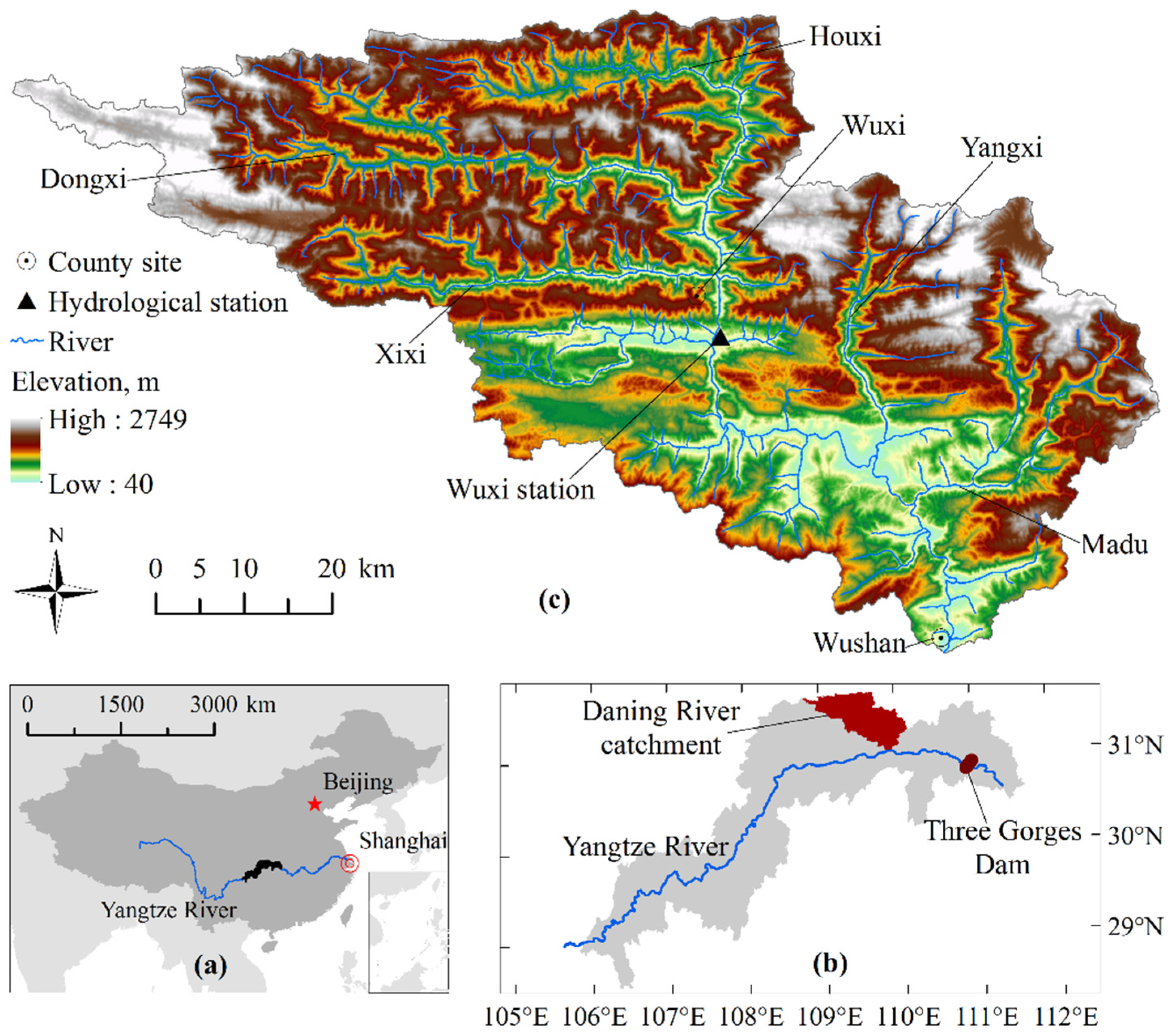
2.1. Study Area

The Daning River catchment has an area of 4400 km2 and is located towards the downstream end of the TGRR, China (Figure 1). The river flows in a southeasterly direction passing through Wuxi and Wushan counties before discharging into the reservoir of the Three Gorges Dam approximately 125 km upstream of the dam site. The river is approximately 250 km long and has five major branches: the Xixi, Dongxi, Houxi, Yangxi and Madu tributaries. The catchment is characterized by variable relief with elevation ranging between 40 m and 2749 m (mean: 1071 m). Slopes are steep and on approximately 53% of the area exceed 25°. Catchment soils are predominantly sandy loams and clays. Forest is the dominant land use, followed by grassland, agricultural land, shrubs, water and urban areas. The catchment has a subtropical monsoon climate with mean annual temperature and precipitation of 15–16 °C and 1000–1300 mm, respectively. Mean discharge at the Wuxi gauging station in the middle reaches of the catchment (Figure 1) is 66 m3·s−1 with seasonal lows of 12 m3·s−1 occurring in December–February and the annual peak in June–August of 199 m3·s−1.

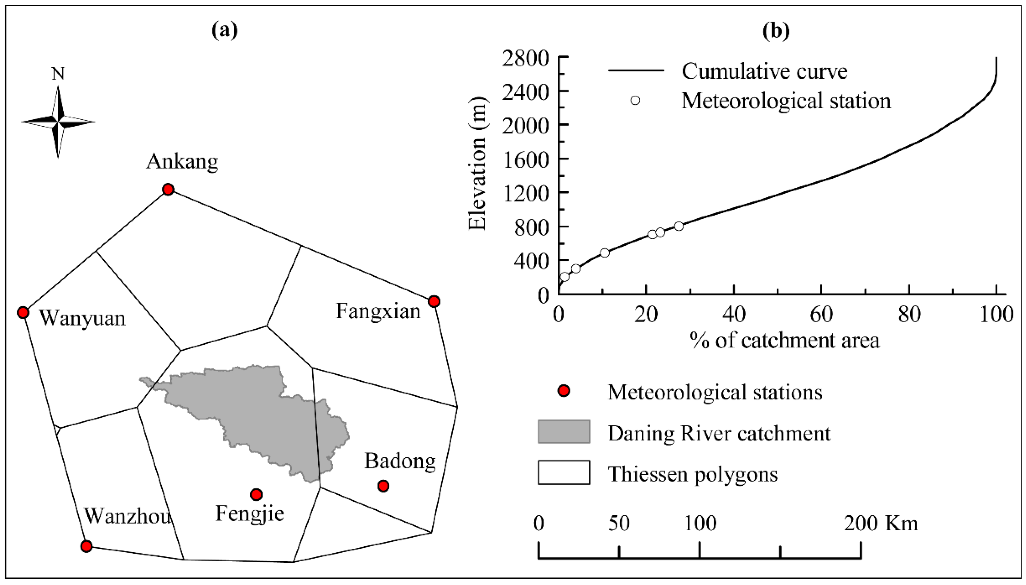
2.2. Data Acquisition

Table 1 summarizes the type, resolution and sources of data employed within the Daning hydrological models. All of the spatial datasets including the Digital Elevation Model, land use, soil and stream network maps were created using ArcGIS 10.1 in the Krasovsky 1940 Albers projection [24]. This produces only small area change in projection transformation so that the simulated catchment area is close to the actual area. Land use was derived from Landsat 7 Thematic Mapper imagery acquired in 1990 and 2004, based on the maximum likelihood supervised classification method combining with prior knowledge of color, tonal and texture features of the landscape in the ENvironment for Visualizing Images (ENVI) program environment. There were six types of land use: forest (1990: 48.6%; 2004: 51.4%), agricultural land (1990: 7.8%; 2004: 11.1%), urban land (1990: 0.2%; 2004: 0.4%), shrub (1990: 7.4%; 2004: 8.9%), grassland (1990: 35%; 2004: 27.2%), and water (1990: 0.9%; 2004: 1.0%). Spatial patterns and total areas of the different land uses changed between 1990 and 2004; forest, agricultural land, shrub, and urban land increased by 5.6%, 41.6%, 20.7%, and 87.7%, respectively, while grassland decreased by 22.4%. Land use was specified as 4-letter SWAT land cover/plant, urban or water land type codes [10]: FRST (forest), AGRL (agricultural land), RNGB (shrub), PAST (grassland), URMD (urban land) and WATR (water cover). There are 34 soil types within the catchment, with the dominant types according to the Chinese genetic soil classification system including yellow soil (27.4%), yellow-brown soil (17.2%), yellow calcareous soil (15%), and brown soil (8.5%). The digital soil map was linked to a user-defined soil database containing soil physical attributes by utilizing a common “Name” field in a look-up table. Some of these soil properties were based on information from the literature [25,26]. The soil-water characteristics that were not available from these sources were initially estimated using pedotransfer functions [27] based on soil texture and organic matter content.

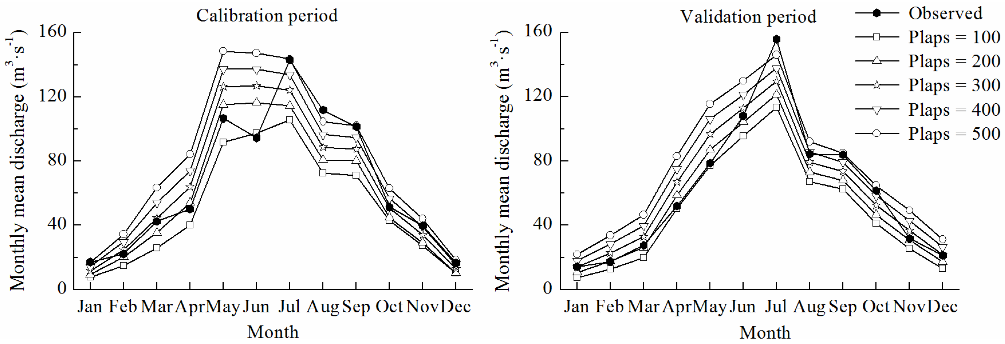
2.3. Model Setup and Formulation of Meteorological Inputs

Hydrological models of the Daning were developed using SWAT2012. Different descriptions of spatial geometric properties within SWAT models resulted in variations in hydraulic characteristics. The impacts of catchment configuration on hydrological model calibration were investigated using 13 alternative thresholds of sub-basin drainage area in the range 17–65 km2 and 12 HRU definitions of area percentage between 0 and 20%. A review of the relative sensitivity of flow parameters in response to these different catchment configurations led to a selection. A threshold drainage area of 30 km2 and HRU percentage cover of 5% were established as the most appropriate spatial resolutions to represent the catchment and avoid model over-parameterization. The Daning catchment was accordingly delineated into 64 sub-basins, with 21 sub-basins above the Wuxi gauging station. Estimations of potential evapotranspiration and surface runoff employed the Hargreaves method [28] and the Soil Conservation Service curve number method [29], respectively.
The Daning catchment typifies the issues associated with the availability of representative meteorological data over mountainous catchments. Data were available from six meteorological stations distributed around the margins of the catchment at distances from the catchment boundary that varied between 20.9 km and 113.6 km (Figure 2a). No long-term records were available from within the catchment (although eight rain gauges within the catchment are operated by county authorities, records are of short duration and are not freely available). As demonstrated in Figure 2b, the six stations from which data are available are at altitudes of 200–800 m, a zone that accounts for only 27% of the total Daning catchment area. Two alternative model setups were defined which reflected varying representation of spatial variations in meteorological inputs. Both employed the same input data and model structure but differed only in the approach used to vary (or not) climate with altitude. The first assigned climate data for the period 1984–2007 directly based on the closest stations to each sub-basin defined within the SWAT2012 model. This, the standard setup of SWAT, is referred to as “without elevation bands”. In this way, precipitation and temperature records for the Fengjie and Badong stations were employed on the basis of the Thiessen polygons shown in Figure 2a with the very small part of the catchment falling in the polygon of the Wanyuan station being assigned records from the first of these two stations. Orographic effects on meteorological inputs were taken into account in the second model setup (“with elevation bands”). Areal climatic inputs were produced from the same meteorological stations but the elevation band approach was employed to simulate orographic effects on precipitation and temperature. Considering a balance between computing efficiency and orographic influence, five elevation bands were defined for which precipitation and temperature were calculated as a function of the respective lapse rate (Plaps and Tlaps, defined as annual adjustments to total precipitation and daily adjustments to maximum and minimum temperatures, respectively) and the difference between the meteorological station’s elevation and the mid-point elevation of each elevation band [10]. The mid-point elevation of the five elevation bands for each sub-basin was calculated using Equation (1):
Ei = Elevmin + (2i − 1) × (ElevmaxElevmin)/2b
where b is the total number of elevation bands defined (b > 1); i is the sequence number of each elevation band (ib); Elevmax and Elevmin is the maximum and minimum elevation of each sub-basin, respectively (m); and Ei is the mid-point elevation of the i elevation band (m).

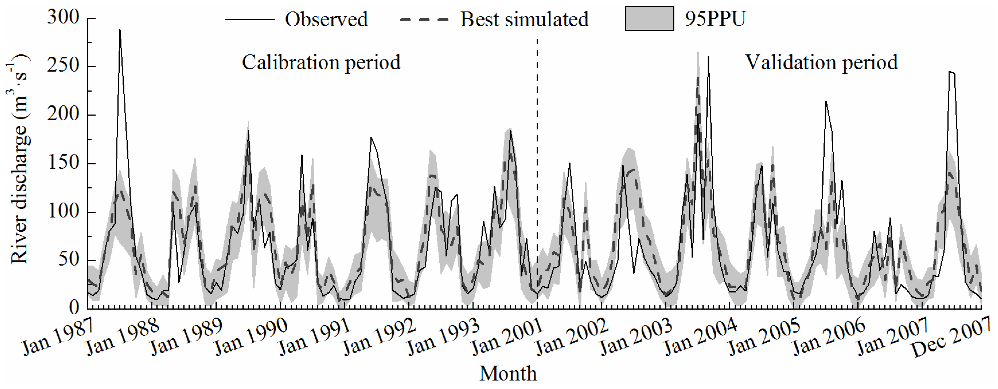
2.4. Model Calibration and Uncertainty Analysis

A global sensitivity analysis [30] was firstly performed to determine the most sensitive parameters impacting simulated river discharge at Wuxi. Details of the parameters included in this analysis and their initial ranges are shown in Table 2. For parameters with moderate sensitivity and relatively low significance, we applied the one-at-a-time sensitivity method to determine if they were selected as calibration terms. Performance of the two model setups (including and excluding elevation bands) were compared prior to calibration since over calibration of parameters to optimize the fit with observations would mask the input data and model structure effects and so would not enable the discrimination of initial model setups [6]. Subsequently the two hydrological models were calibrated independently with the Sequential Uncertainty Fitting program (SUFI2) being used for model calibration and uncertainty analysis. SUFI2, which is available within the SWAT Calibration and Uncertainty Program (SWAT-CUP) [30], employs the concept of inverse modeling and adopts the gradient approach but with modifications to enable a global search with Latin hypercube sampling. It overcomes the weaknesses of the gradient procedure and the global search algorithm that are respectively applied in Generalized Likelihood Uncertainty Estimation (GLUE) and Parameter Solution (ParaSol) [31]. These issues include the sensitivity of the gradient method to the initial parameter values that can lead to local minima, problems associated with including a large number of parameters, and computational inefficiency in global procedures, such as shuffled complex and genetic algorithms [32].
The model calibration process consisted of four iterations, each of which was performed with 480 Latin Hypercube samples for the period 1987–1993 (with 1984–1986 used as a model warm-up period). Land use data from 1990 were used for this simulation period. In the first iteration, an appropriate range for each parameter was provided to prevent model over calibration, being physically meaningful to catchment conditions. In the case of the “with elevation bands” model setup, the initial ranges of Plaps and Tlaps were determined by plotting mean annual precipitation and mean annual temperature against elevation using data from stations in the wider region (156 stations, the furthest station at distance of 354 km from the catchment boundary). Parameter ranges for subsequent iterations were narrowed following results from the previous iteration. This process produced a best-range for each parameter and aimed at obtaining the smallest parameter uncertainty. Calibrated models were validated using the period 2001–2007 (warm up: 1998–2000) with the 2004 land use, but keeping all other inputs the same. The use of the more recent land use for this period was justified due to the potential effects of land use changes on hydrological processes. Given the temporal changes in land cover experienced in the Daning, this approach was designed to limit the influence of incorrectly specified land use upon model performance in the validation period. Simulated discharges for the validation period were obtained by performing 480 model runs for each model setup drawing parameter values from the final ranges obtained at the end of the calibration process. Comparisons were made between the simulated discharges from the calibrated models with and without elevation bands, and observations from the Wuxi gauging station.
The Nash–Sutcliffe efficiency index (NSE) [33] was employed as the objective function in calibrations. When calculating the NSE value, the model also generates the P-factor and R-factor to quantify model prediction uncertainty. These two indices are effective measures for model goodness-of-fit testing. The P-factor, which expresses the proportion of observations covered by the 95% prediction uncertainty (95PPU) band, can vary between 0 and 100%. Bracketing most of the observed data within the 95PPU band indicates that a model has been well calibrated [34]. The R-factor describes the relative width of 95% probability level. The ideal value is 0, which would indicate that there is no uncertainty in model outputs. However, it implies that fewer flow observations were included in the 95PPU band. Therefore a compromise between the P-factor and R-factor was made with an R-factor value closer to 1 being desirable when the P-factor was no less than 75% [34]. One further performance measure was considered to evaluate the robustness of the calibration. Fd was calculated as the differences between the simulated and observed annual discharges. Based on the values of NSE and Fd, model performance was classified using the scheme of Henriksen et al. [35] into five levels ranging between excellent and very poor (Table 3).

3. Results

The sensitivity analyses undertaken for the model incorporating elevation bands showed that the most sensitive parameters were Plaps, Tlaps and CH_K1 at the subbasin level, and SURLAG, SMFMX, TIMP and SNO50COV at the basin level. At the HRU level the following parameters were most sensitive: Canmx, ESCO, OV_N, HRU_SLP and SLSUBBSN. Other sensitive parameters were Sol_K(1) and Sol_AWC(1) (soil parameters), CH_K2 and CH_N2 (channel parameters), GWQMN, GW_Delay and GW_REVAP (groundwater parameters) and CN2, a management parameter. The physical meanings and relative sensitivity of these parameters are summarized in Table 2. The model without elevation band was sensitive to the same parameters with the exclusion of Plaps and Tlaps, which were not included in the model setup, with an additional parameter, Alpha_bf (baseflow alpha factor), being identified as the second most sensitive parameter. The large sensitivity of the model that included elevation band to the Plaps parameter demonstrates the range of uncertainty associated with altitudinal variations in precipitation. This is illustrated in Figure 3 that presents the impact of variations in Plaps within the calibrated model upon simulated discharge. An increase of 100 H2O·mm·km−1·year−1 in the Plaps value resulted in a monthly mean discharge increase of 15.2% and 15.9% on average in the calibration and validation periods, respectively. Deviation of simulated discharges from the observations ranged between −54.3% and 68.2% in calibration period, and between −47.4% and 93.6% in validation period. Application of small Plaps value causes the model to reproduce the observed low flows, but the peak flows are underestimated. Conversely, larger Plaps values enable the model to capture the observed peaks but results in the overestimation of low flows. The final calibrated value of 278 H2O·mm·km−1·year−1 was selected to reproduction of both peaks and low flows.
Employing elevation bands to adjust precipitation and temperature with altitude and providing initial ranges of lapse rates produced better model performance for the period 1987–1993 compared to the model without elevation bands (Table 4). The value of NSE increased by at least 0.11 for daily simulation of river flow prior to calibration. The 1st and 2nd calibration iterations produced similar R-factors and the P-factor values were comparable for the model without elevation bands. An additional 11% of daily observations were included in the 95PPU. For behavioral simulations (defined within SWAT-CUP using a NSE threshold of 0.3) with elevation bands, an additional 3.9% of observations were within the 95PPU while the uncertainty reduced by 7.6%. Although the P-factors are not directly comparable after calibration for the two model setups since the R-factors are different, the higher NSE values illustrates that the hydrological model which includes elevation bands improves the simulation accuracy. This superior performance is quantified in Table 4. The NSE value of the “without elevation bands” model setup is classified as indicative of “poor” performance. This improves to “very good” once altitudinal variations are included. Model validation using the period 2001–2007 also shows that the inclusion of elevation bands results in performance that is classified as “fair” compared to “poor” if altitudinal variations in meteorological inputs are excluded.
The calibrated ranges and best-fit values of the parameters for the model with elevation bands are shown in Table 2. The range in parameter values is considerably narrower following calibration compared to the initial range of values. Parameter uncertainty has been greatly reduced. The 95PPU band includes 85% and 75% of the monthly observations in the calibration and validation periods, respectively. The corresponding R-factors are 0.87 and 0.76, respectively. This performance again demonstrates the good calibration of the SWAT model setup which includes elevation bands. The calibrated model reproduced the observed mean monthly discharges reasonably well with the exception of the seasonal peaks in 1987 and 1991 of the calibration period and 2004, 2005 and 2007 of the validation period (Figure 4). Comparisons of observed and simulated annual discharges demonstrate a difference of between 2.4% and 26.4% for the calibration period and between 5.1% and 45.3% for the validation period (Table 3). The Fd performances are in the class of “fair” to “excellent” with the exception of 1987, 1988, 2005 and 2006 (“poor”) and 2002 (“very poor”).
Figure 5 shows the observed river regime (the mean monthly river flow) of the Daning River at Wuxi for both the calibration and validation periods as well as the corresponding simulated regimes. Although the model that excludes elevation bands reproduces the observed seasonality in river discharge, considerable underestimation of as much as 49% (mean: 29%) is evident throughout the year. In particular, a substantial error occurs in the simulation of seasonal peak discharge. The introduction of elevation bands to the hydrological model leads to an overall increase in simulated discharges. The mean difference between observed and simulated discharges declines to 12.6%, although peak July discharges are underestimated by 16.8%.

4. Discussion

Focusing efforts on sensitive parameters improves the efficiency of model calibration. The specification of precipitation and temperature lapse rates with elevation bands enables orographic effects upon precipitation (increases with altitude per km) and temperature (decreases with altitude per km), and in turn, evapotranspiration (declines with altitude) to be represented. This approach adjusts the potential underestimation of precipitation into the Daning catchment which results from the altitude of the meteorological stations at elevations which are not representative of the wider catchment while also correcting water removal by evapotranspiration and influencing simulated snow accumulation, sublimation and melting processes at higher altitudes. These two lapse rate parameters together with the other sensitive parameters (Table 2) determined the water allocation between infiltration or snow pack, surface runoff and evapotranspiration. The importance of CN2, Canmx, ESCO, Sol_AWC, Sol_K, and GWQMN parameters in the Daning SWAT hydrological model was also demonstrated by Shen et al. [36] who applied the one-factor-at-a-time parameter sensitivity analysis method. However, this earlier study did not differentiate the CN2 parameter of one land use from another while within the Daning model of the current study the CN2 parameter was distributed according to land over. They also did not consider snow-related processes, which are crucial to the hydrology of many mountain areas including the Daning catchment as confirmed by this study. This was the result of the exclusion of altitude dependent climate inputs. The time series of temperature they used was normally above zero and since temperature did not change with altitude there was never any snow simulated by their model.
Employing elevation bands to vary precipitation and temperature with altitude led to large improvements in the simulation of river discharge, with NSE increasing by 0.22 in 1987–1993 and 0.17 in 2001–2007. The calibrated model reproduced the observed monthly streamflow to an acceptable level. The larger discrepancies in simulated seasonal peak flows during the periods 1987–1993 and 2001–2007 (Figure 4) may have resulted from the spatial variability of precipitation, which has a particular impact on peak flow simulations in mountain area as confirmed through rainfall gradient experiments [9]. Spatial representation of precipitation based on sparse ground observations and an unvarying precipitation lapse rate across the catchment may be one cause of the streamflow underestimation. Precipitation lapse rates may vary over relatively short-distances and over time [37]. In addition, differences between observed and simulated peak discharges could be attributed to the simulation of snowmelt processes. The actual snowmelt water volume depends on the potential meltwater rate and the extent of snow coverage [8]. Altitudinally varying temperature determines the potential snowmelt rate which changes in response to snowpack conditions, such as snowpack temperature and free water content [38]. The most influential variables include snowpack density, solar radiation intensity, and snow surface albedo [8,10]. SMFMX and TIMP, which were identified as sensitive parameters in the model of the Daning catchment, account for the impacts of these factors on snowmelt. During the melt season, snow coverage and hence the contribution of meltwater was progressively reduced. This was determined by a snow cover depletion curve [10], which was ultimately determined by the parameter SNO50COV. It is possible that a uniform temperature lapse rate across the catchment combined with these snowmelt related parameters impacted the simulation of snowmelt runoff.
Although it is inappropriate to directly compare P-factor values when R-factors are different, the calibrated model with elevation bands explicitly reduced the prediction uncertainty compared to earlier model iterations. Parameter sets within the calibrated ranges produced similar overall performance, demonstrating the phenomenon of equifinality in inverse model optimization [39], being larger than the NSE behavioral threshold (0.3) for daily streamflow modeling. The defined behavioral threshold of NSE helped to eliminate unsatisfactory simulations, and thus reduced the parameter uncertainty. Adjusting climatic inputs with elevation using SWAT’s elevation band procedure integrated the uncertainty of observational climate with parameter uncertainty of the Plaps and Tlaps terms. It transferred the input uncertainty to parameter uncertainty. The calibrated Plaps and Tlaps parameters to some extent reduced the uncertainty associated with climatic inputs. The prediction uncertainty produced by SUFI2 reflects a combination of uncertainties derived from the description of natural processes, model inputs and estimation of parameter values. It differs from the uncertainty assessment gained by the first-order error analysis or Monte Carlo method undertaken by Shen et al. [36], which only generated parameter uncertainty of a model of the Daning catchment. As a tool for water resources planning and management, the available combined uncertainty is required to explicitly understand the reliability of model outputs.
Efforts to reduce uncertainty in Daning River flow prediction should be focused on the problems related to spare climatological observations in a region with large variations in elevation and where a large proportion of the modeled catchment has elevations which are higher than the existing meteorological stations. Totally error-free observations are difficult to obtain, but increasing the spatial resolution and data quality are technically possible. Increasing the density of ground observation within the Daning catchment, and indeed the wider TGRR, including the collection of data from higher altitudes would enhance the ability of station records to represent spatial variability in meteorological condition although it would not be without logistical challenges. Use of elevation bands may address some deficiencies in data availability. However, results from this study do demonstrate that systematic differences between observed and simulated discharges remain (e.g., Figure 4). Approximate expressions of precipitation and temperature even with the elevation bands mainly depend on the meteorological observations. Improvements in the meteorological observation network across the Daning River catchment are likely to provide a better approximation of variations in meteorological conditions across the catchment.

5. Conclusions

Application of the SWAT2012-SUFI2 with the inclusion of elevation bands as a calibration term addressed some of the deficiencies associated with uncertainty in meteorological inputs when modeling data-sparse mountainous catchments. It led to an improved performance of the Daning model in simulating daily river discharge, with the NSE increasing by >0.11 prior to calibration. The prediction uncertainty was reduced compared to earlier calibration iterations. An additional 11% of the daily observations were included in the 95PPU compared to the model without elevation bands. For behavioral simulations, an additional 3.9% of observations were within the 95PPU while the uncertainty reduced by 7.6% in the model with elevation bands. The calibrated model with elevation bands resulted in the performance being classified as “very good” compared to “poor” for the model in which altitudinal variations in meteorological conditions were excluded. Prediction uncertainty was acceptable (P-factor = 85%, R-factor = 0.87).
For mountainous catchments, such as those within the TGRR, where meteorological inputs are limited in spatial extent and derived from climate stations in relatively low lying locations, the application of elevation bands provides one means of representing altitudinal variations in meteorological conditions within hydrological models. Although systematic differences between simulated discharges and the observations remain, improved model performance and the quantification of prediction uncertainty would support water resources planning and management in poorly observed mountainous areas. Improvements in the density of ground observation, including the collection of data from higher altitudes, would be necessary to improve model performance and guide selection of the lapse rates employed within the hydrological models of these catchments.

Acknowledgments

This research was sponsored by the National Natural Science Foundation of China (Grant No. 41271500 and 40871238), the Key Research Program of the Chinese Academy of Sciences (Grant No. KZZD-EW-10-04 and KZCX1-YW-08-01), the “135” Key Program of the Nanjing Institute of Geography & Limnology, Chinese Academy of Sciences (Grant No. NIGLAS2012135005), and the Graduate School of UCL and the Royal Geographical Society (with the IBG).

Author Contributions

Yan Li developed the SWAT2012-SUFI2 model for the Daning River catchment and wrote the initial draft of this manuscript; Julian R. Thompson reviewed and commented on the model results and writing; and Hengpeng Li contributed materials and provided valuable insights to refine this research.

Conflicts of Interest

The authors declare no conflict of interest.

References

  1. Palmer, M.A.; Reidy Liermann, C.A.; Nilsson, C.; Flörke, M.; Alcamo, J.; Lake, P.S.; Bond, N. Climate change and the world's river basins: Anticipating management options. Front. Ecol. Environ. 2008, 6, 81–89. [Google Scholar] [CrossRef]
  2. Strauch, M.; Lima, J.E.F.W.; Volk, M.; Lorz, C.; Makeschin, F. The impact of best management practices on simulated streamflow and sediment load in a central brazilian catchment. J. Environ. Manag. 2013, 127, S24–S36. [Google Scholar] [CrossRef] [PubMed]
  3. Faramarzi, M.; Abbaspour, K.C.; Vaghefi, S.A.; Farzaneh, M.R.; Zehnder, A.J.; Srinivasan, R.; Yang, H. Modelling impacts of climate change on freshwater availability in Africa. J. Hydrol. 2013, 480, 85–101. [Google Scholar] [CrossRef]
  4. Du, J.; Rui, H.; Zuo, T.; Li, Q.; Zheng, D.; Chen, A.; Xu, Y.; Xu, C.Y. Hydrological simulation by swat model with fixed and varied parameterization approaches under land use change. Water Resour. Manag. 2013, 27, 2823–2838. [Google Scholar] [CrossRef]
  5. Wijesekara, G.; Gupta, A.; Valeo, C.; Hasbani, J.-G.; Qiao, Y.; Delaney, P.; Marceau, D. Assessing the impact of future land-use changes on hydrological processes in the elbow river watershed in southern Alberta, Canada. J. Hydrol. 2012, 412, 220–232. [Google Scholar] [CrossRef]
  6. Faramarzi, M.; Srinivasan, R.; Iravani, M.; Bladon, K.D.; Abbaspour, K.C.; Zehnder, A.J.; Goss, G.G. Setting up a hydrological model of Alberta: Data discrimination analyses prior to calibration. Environ. Model. Softw. 2015, 74, 48–65. [Google Scholar] [CrossRef]
  7. Houska, T.; Multsch, S.; Kraft, P.; Frede, H.-G.; Breuer, L. Monte Carlo-based calibration and uncertainty analysis of a coupled plant growth and hydrological model. Biogeosciences 2014, 11, 2069–2082. [Google Scholar] [CrossRef]
  8. Fontaine, T.; Cruickshank, T.; Arnold, J.; Hotchkiss, R. Development of a snowfall–snowmelt routine for mountainous terrain for the soil water assessment tool (swat). J. Hydrol. 2002, 262, 209–223. [Google Scholar] [CrossRef]
  9. Schäppi, B. Measurement and Analysis of Rainfall gradients Along a Hillslope Transect in the Swiss Alps; ETH Zurich: Zurich, Switzerland, 2013. [Google Scholar]
  10. Neitsch, S.L.; Arnold, J.G.; Kiniry, J.R.; Williams, J.R. Soil and Water Assessment tool, Theoretical Documentation: Version 2009; Texas Water Resources Institute, Texas A & M University System College Station: TX, USA, 2011; pp. 1–647. [Google Scholar]
  11. Buytaert, W.; Celleri, R.; Willems, P.; Bièvre, B.D.; Wyseure, G. Spatial and temporal rainfall variability in mountainous areas: A case study from the south Ecuadorian Andes. J. Hydrol. 2006, 329, 413–421. [Google Scholar] [CrossRef] [Green Version]
  12. Goovaerts, P. Geostatistical approaches for incorporating elevation into the spatial interpolation of rainfall. J. Hydrol. 2000, 228, 113–129. [Google Scholar] [CrossRef]
  13. Gali, R.K.; Douglas-Mankin, K.R.; Li, X.; Xu, T. Assessment of nexrad p3 data on streamflow simulation using swat model in an agricultural watershed. J. Hydrol.Eng. 2010, 17. [Google Scholar] [CrossRef]
  14. Cunha, L.K.; Mandapaka, P.V.; Krajewski, W.F.; Mantilla, R.; Bradley, A.A. Impact of radar-rainfall error structure on estimated flood magnitude across scales: An investigation based on a parsimonious distributed hydrological model. Water Resour. Res. 2012, 48, 1–22. [Google Scholar] [CrossRef]
  15. Bitew, M.M.; Gebremichael, M. Evaluation of satellite rainfall products through hydrologic simulation in a fully distributed hydrologic model. Water Resour. Res. 2011, 47, 1–11. [Google Scholar] [CrossRef]
  16. Bitew, M.; Gebremichael, M. Assessment of satellite rainfall products for streamflow simulation in medium watersheds of the Ethiopian highlands. Hydrol. Earth Syst. Sci. 2011, 15, 1147–1155. [Google Scholar] [CrossRef]
  17. Gourley, J.J.; Hong, Y.; Flamig, Z.L.; Wang, J.; Vergara, H.; Anagnostou, E.N. Hydrologic evaluation of rainfall estimates from radar, satellite, gauge, and combinations on ft. Cobb basin, Oklahoma. J. Hydrometeorol. 2011, 12, 973–988. [Google Scholar] [CrossRef]
  18. Kwon, S.; Jung, S.-H.; Lee, G. Inter-comparison of radar rainfall rate using constant altitude plan position indicator and hybrid surface rainfall maps. J. Hydrol. 2015, 531, 234–247. [Google Scholar] [CrossRef]
  19. Viviroli, D.; Zappa, M.; Gurtz, J.; Weingartner, R. An introduction to the hydrological modelling system prevah and its pre- and post-processing-tools. Environ. Model. Softw. 2009, 24, 1209–1222. [Google Scholar] [CrossRef]
  20. Thompson, J.; Green, A.; Kingston, D.; Gosling, S. Assessment of uncertainty in river flow projections for the Mekong river using multiple GCMs and hydrological models. J. Hydrol. 2013, 486, 1–30. [Google Scholar] [CrossRef]
  21. Masih, I.; Maskey, S.; Uhlenbrook, S.; Smakhtin, V. Assessing the impact of areal precipitation input on streamflow simulations using the SWAT model. J. Am. Water Resour. Assoc. 2011, 47, 179–195. [Google Scholar] [CrossRef]
  22. Bosshard, T.; Zappa, M. Regional parameter allocation and predictive uncertainty estimation of a rainfall-runoff model in the poorly gauged three gorges area (PR China). Phys. Chem. Earth Parts A/B/C 2008, 33, 1095–1104. [Google Scholar] [CrossRef]
  23. Wu, Y.J.; Gough, W.A.; Jiang, T.; Kung, H.T. The variation of floods in the middle reaches of the Yangtze river and its teleconnection with all niño events. Adv. Geosci. 2006, 6, 201–205. [Google Scholar] [CrossRef]
  24. Zeng, T.; Zhang, Z.; Zhao, X.; Wang, X.; Zuo, L. Evaluation of the 2010 MODIS collection 5.1 land cover type product over China. Remote Sens. 2015, 7, 1981–2006. [Google Scholar] [CrossRef]
  25. Soil Survey Office of Chongqing. Soil Species of Chongqing; Chongqing Soil Office Press: Chongqing, China, 1986.
  26. Agriculture and Animal Husbandry Department of Sichuan; Soil survey office of Sichuan. Soil Species of Sichuan; Sichuan Science & Technology Press: Chengdu, Sichuan, China, 1994.
  27. Saxton, K.E.; Rawls, W.J. Soil water characteristic estimates by texture and organic matter for hydrologic solutions. Soil Sci. Soc. Am. J. 2006, 70, 1569–1578. [Google Scholar] [CrossRef]
  28. Hargreaves, G.H.; Samani, Z.A. Reference crop evapotranspiration from temperature. Appl. Eng. Agric. 1985, 1, 96–99. [Google Scholar] [CrossRef]
  29. USDA Soil Conservation Service. National Engineering Handbook; Section 4, Hydrology; U.S. Department of Agriculture: Washington, DC, USA, 1972.
  30. Abbaspour, K.C. Swat-Cup2: Swat Calibration and Uncertainty Programs—A User Manual; Department of Systems Analysis, Swiss Federal Institute of Aquatic Science and Technology: Dübendorf, Switzerland, 2012. [Google Scholar]
  31. Yang, J.; Reichert, P.; Abbaspour, K.C.; Xia, J.; Yang, H. Comparing uncertainty analysis techniques for a swat application to the chaohe basin in china. J. Hydrol. 2008, 358, 1–23. [Google Scholar] [CrossRef]
  32. Gupta, H.V.; Bastidas, L.A.; Vrugt, J.A.; Sorooshian, S. Multiple criteria global optimization for watershed model calibration. Water Sci. Appl. 2003, 6, 125–132. [Google Scholar]
  33. Nash, J.E.; Sutcliffe, J.V. River flow forecasting through conceptual models part I—A discussion of principles. J. Hydrol. 1970, 10, 282–290. [Google Scholar] [CrossRef]
  34. Abbaspour, K.C.; Yang, J.; Maximov, I.; Siber, R.; Bogner, K.; Mieleitner, J.; Zobrist, J.; Srinivasan, R. Modelling hydrology and water quality in the pre-alpine/alpine Thur watershed using swat. J. Hydrol. 2007, 333, 413–430. [Google Scholar] [CrossRef]
  35. Henriksen, H.; Troldborg, L.; Højberg, A.; Refsgaard, J. Assessment of exploitable groundwater resources of Denmark by use of ensemble resource indicators and a numerical groundwater-surface water model. J. Hydrol. 2008, 348, 224–240. [Google Scholar] [CrossRef]
  36. Shen, Z.Y.; Hong, Q.; Yu, H.; Liu, R.M. Parameter uncertainty analysis of the non-point source pollution in the Daning river watershed of the three gorges reservoir region, china. Sci. Total Environ. 2008, 405, 195–205. [Google Scholar] [CrossRef] [PubMed]
  37. Leemans, R.; Cramer, W.P. The IIASA Database for Mean Monthly Values of Temperature, Precipitation, and Cloudiness on a Global Terrestrial Grid; International Institute for Applied Systems Analysis: Laxenburg, Austria, 1991. [Google Scholar]
  38. Martinec, J.; Rango, A. Parameter values for snowmelt runoff modelling. J. Hydrol. 1986, 84, 197–219. [Google Scholar] [CrossRef]
  39. Beven, K.; Freer, J. Equifinality, data assimilation, and uncertainty estimation in mechanistic modelling of complex environmental systems using the glue methodology. J. Hydrol. 2001, 249, 11–29. [Google Scholar] [CrossRef]
Figure 1. Location of the Daning River catchment: (a) map of China; (b) Three Gorges Reservoir Region; and (c) Daning River Catchment.
Water 08 00073 g001
Figure 2. (a) National meteorological stations around the Daning River catchment and their Thiessen polygons; and (b) the catchment’s elevation compositions and stations’ elevations.
Water 08 00073 g002
Figure 3. Observed and simulated monthly mean discharges impacted by variations in Plaps in the calibration and validation periods.
Water 08 00073 g003
Figure 4. Observed, best simulated hydrographs and 95PPU band in calibration and validation periods.
Water 08 00073 g004
Figure 5. Observed and simulated (with and without elevation bands) river regimes for the Daning River at Wuxi over the period of calibration and validation.
Water 08 00073 g005
Table 1. Data types, resolution and data sources.
Data TypeResolutionData sourceDataset Link
Digital elevation model30 × 30 m2Advanced Spaceborne Thermal Emission and Reflection Radiometer global, U.S. Geological Surveyhttp://www.usgs.gov (accessed on 5 October 2010)
Land use map30 × 30 m2Landsat 7 Thematic Mapper, U.S. Geological Surveyhttp://www.usgs.gov (accessed on 5 October 2010)
Soil map1:250,000Institute of Soil Science, Chinese Academy of Scienceshttp://www.soil.csdb.cn (accessed on 25 November 2011)
Climate dataDailyChina Meteorological Administrationhttp://www.cma.gov.cn/2011qxfw/2011qsjgx (accessed on 1 July 2012)
River dischargesDailyBureau of Hydrology, Yangtze Water Resources Commissionhttp://www.cjw.gov.cn/Index.html (accessed on 5 August 2010)
Table 2. Physical meanings, sensitivity, initial and calibrated ranges of flow parameters.
Flow ParameterPhysical Meaning (Unit)Relative SensitivityInitial RangesCalibrated RangesBest-Fit
v*_Plaps.subPrecipitation lapse rate (mm·H2O·km−1)−1.17[150, 700][245, 498]278
v_Tlaps.subTemperature lapse rate (°C·km−1)−0.91[–10, 0][−3.9, −0.9]−1.3
v_CH_K1.subEffective hydraulic conductivity in tributary channel alluvium (mm·h1)0.03[5, 150][59.7, 114.3]82.8
r**_CN2.mgt_FRSTSCS runoff curve number for moisture condition 2 of forest, agricultural land, and typical grassland0.61[−0.5, 0.5][−0.75, −0.17]−0.67
r_CN2.mgt_AGRL−0.60[−0.5, 0.5][0.08, 0.65]0.21
r_CN2.mgt_PAST0.32[−0.5, 0.5][0.19, 0.68]0.52
v_Canmx.hruMaximum canopy storage (mm·H2O)−0.65[0, 100][25.6, 60]26.5
v_ESCO.hruSoil evaporation compensation factor−0.36[0.01, 1.0][0.52, 0.81]0.78
r_OV_N.hruManning’s “n” value for overland flow−0.17[−0.5, 0.5][−0.43, 0.11]−0.36
r_HRU_SLP.hruAverage slope steepness (m·m1)−0.11[−0.5, 0.5][−0.18, 0.47]0.093
r_SLSUBBSN.hruAverage slope length (m)0.07[−0.5, 0.5][−0.19, 0.11]-0.15
v_SURLAG.bsnSurface runoff lag coefficient0.52[1, 24][6.3, 13.4]12.0
v_SMFMX.bsnMelt factor for snow on 21 June (mm·H2O/°C-day)−1.02[0, 10][3.1, 6.7]4.92
v_TIMP.bsnSnow pack temperature lag factor−0.79[0, 1][0.49, 1]0.59
v_SNO50COV.bsnRatio of snow water equivalent at 50% areal snow coverage to its threshold at 100% snow cover−3.41[0, 1][0.18, 0.56]0.49
v_CH_K2.rteEffective hydraulic conductivity in main channel alluvium (mm·h1)−1.28[0, 150][0, 58.6]28.0
v_CH_N2.rteManning’s “n” value for the main channel1.00[0, 0.2][0.028, 0.11]0.086
r_Sol_K(1).solSaturated hydraulic conductivity (mm·h1)−0.26[−0.5, 0.5][0.2, 0.76]0.63
r_Sol_AWC(1).solAvailable water capacity of the soil layer (mm·H2O·mm1 soil)−0.05[−0.5, 0.5][0.16, 0.69]0.63
v_GWQMN.gwThreshold depth of water in the shallow aquifer required for return flow to occur (mm·H2O)1.70[0, 5000][520,2010]984.1
v_GW_REVAP.gwGroundwater “revap” coefficient−2.37[0. 0, 0.2][0.04, 0.2]0.10
v_GW_DELAY.gwGroundwater delay time (days)−1.00[0, 500][8.33, 212.8]124
Note: * and ** parameter value is replaced by given value and multiplied by (1+ a given value), respectively.
Table 3. Differences between simulated and observed annual discharges and model performance.
YearFd (%)Fd PerformanceYearFd (%)Fd Performance
1987−21.5 *poor200112.4Fair
198826.4poor200245.3very poor
198915.8fair2003−6.7 *very good
19905.3very good20046.4very good
1991−2.8 *excellent2005−32.1 *Poor
19922.44excellent200625.0Poor
1993-3.1 *excellent2007–5.1 *very good
Performance IndicatorExcellentVery GoodFairPoorVery Poor
NSE>0.850.65–0.850.50–0.650.20–0.50<0.20
Fd<5%5%–10%10%–20%20%–40%>40%
Note: * underestimate of simulated annual discharge comparing with the observation.
Table 4. Model performances of daily and monthly streamflows with and without elevation bands.
PeriodProcedureGoodness-of-Fit Measures“Without” Model Setup“With” Model Setup
1987–1993Prior calibration (daily)NSE0.250.36
1st and 2nd Iteration (daily)NSE0.29 (1st), 0.33 (2nd)0.42 (1st), 0.45 (2nd)
P-factor (%)55 (1st), 66 (2nd)77 (1st), 80 (2nd)
R-factor0.39 (1st), 0.37 (2nd)0.66 (1st), 0.61 (2nd)
Calibration (monthly)NSE0.470.69
P-factor (%)4985
R-factor0.460.87
2001–2007Validation (monthly)NSE0.420.59
P-factor (%)2675
R-factor0.130.76

