Assessment of Climate Change Impacts on Water Quality in a Tidal Estuarine System Using a Three-Dimensional Model

Abstract

Climate change is one of the key factors affecting the future quality and quantity of water in rivers and tidal estuaries. A coupled three-dimensional hydrodynamic and water quality model has been developed and applied to the Danshuei River estuarine system in northern Taiwan to predict the influences of climate change on water quality. The water quality model considers state variables including nitrogen, phosphorus, organic carbon, and phytoplankton as well as dissolved oxygen, and is driven by a three-dimensional hydrodynamic model. The hydrodynamic water quality model was validated with observational salinity distribution and water quality state variables. According to the analyses of statistical error, predictions of salinity, dissolved oxygen, and nutrients from the model simulation quantitatively agreed with the observed data. The validated model was then applied to predict water quality conditions as a result of projected climate change effects. The simulated results indicated that the dissolved oxygen concentration was projected to significantly decrease whereas nutrients will increase because of climate change. Moreover, the dissolved oxygen concentration was lower than 2 mg/L in the main stream of the Danshuei River estuary and failed to meet the water quality standard. An appropriate strategy for effective water quality management for tidal estuaries is needed given the projected persistent climate trends.

1. Introduction

Estuaries are among the world’s vital aquatic resources. They provide food resources and a habitat for ecologically and economically important fish and shellfish species, recreational regions, educational and scientific experiences, and other important ecosystem services [1,2,3,4,5]. For example, the Guandu Natural Park in Taipei city, which is located at the confluence of the Danshuei River and the Keelung River, serves as an educational purpose and scientific experience [6]. Ecosystem services are fundamental life-support processes upon which all organisms depend [7]. Two ecosystem services that estuaries provide are water filtration and habit protection. However, adverse impacts on the estuarine ecosystem by environmental perturbations (e.g., anthropogenic nutrient loading, land use change, hydrological modification) have been widely reported [8,9,10]. The adverse impacts include impaired water quality, habitat loss, and diminished resources [11]. These perturbations result in declining water quality and deleterious changes in ecosystem structure and tropic dynamics [12,13]. The deleterious water quality subsequently produces the problems of odor, aesthetics, human pathogens, and increased public health risk. For example, McKibben et al. [14] reported that harmful algal blooms are proliferations of microscopic algae that harm the environment by producing toxins that accumulate in shellfish or fish, or through the accumulation of biomass that in turn affects co-occurring organisms and alters food webs in negative ways. Impacts include human illness and mortality following direct consumption or indirect exposure to toxic shellfish or toxins in the environment.

Climate change occurs naturally, but human population growth and associated land-cover deforestation and burning of fossil fuel have substantially accelerated the increase in greenhouse gases (CO₂, CH₄, N₂O, etc.). The elevated concentration of CO₂ and other greenhouse gases from anthropogenic activities have caused warming of the global climate by modifying radiative forcings, and continued changes will result in climate shifts [15,16,17,18]. Feng et al. [19] used model-projected future surface temperature and precipitation to examine the change/shifts of climate types over the global land area. They concluded that compared to the present-day condition, the boreal winter temperature over the global land area is projected to increase by 3‒12 °C by 2071‒2100 under a high emission scenario. Strong warming (>8 °C) appears along the Arctic coastal regions, moderate warming (5‒7 °C) appears in the mid-latitude of the Northern Hemisphere, while the warming in the tropical and the Southern Hemisphere is relatively smaller (<5 °C). The projected warming in the boreal summer is much weaker (3‒6 °C). Xin et al. [20] studied climate change projections over East Asia under various representative concentration pathway (RCP) scenarios using simulations conducted with the Beijing Climate Center Climate System Model for the Coupled Model Intercomparison Project phase 5. Under all RCPs, including RCP2.6, RCP4.5, RCP6.0, and RCP8.5, the East Asian climate is found to be warmer and wetter in the 21st century than the present climatology (1986‒2005). For 2080‒2099, the East Asian mean surface air temperature is higher than for present climatology by 0.98 °C (4.4%) under RCP2.6, 1.89 °C (7.7%) under RCP4.5, 2.47 °C (7.1%) under RCP6.0, and 4.06 °C (9.1%) under RCP8.5.

The impacts of climate change on human health have been widely reported [21,22,23]. Numerous studies project greater morbidity and mortality from direct exposure, as well as greater health risks due to decreased air quality, water-borne disease, and other infectious diseases [23,24]. Impacts of climate change on river and estuarine systems provide a subject of active research [25,26,27] because of the importance of water resources for human activities. Potential impacts of climate change on hydrology cover changes in runoff discharge, river flow, and groundwater storage [28]. Impacts on water quality include many factors (physical, including temperature, turbidity; chemical, including pH and concentration; biological, including biodiversity and species abundance across the entire food web from microbial pools and macrophytes up to fishes). With respect to water quality, most climate change impacts can be attributed to changes in either discharge—which controls dilution, flow velocity, and residence time—or water temperature. The impact of climate change on river and estuarine water quality is also heavily dependent on the future evolution of human activities (pollutions, withdrawals, etc.), so the direct influence of climate change may end up being relatively small [29].

The impact of climate change on estuaries has been reviewed by Robins et al. [30], who reported that potential changes to physical processes include flooding and coastal squeeze, caused by increased sea level rise, changing surge and wave climates, and changing river flow events. Sea level rise will cause a shift towards net sediment accretion, but with reduced transport in UK estuaries. Turbulent mixing that is critical for water quality and coastal ecology is controlled by river flow variability. Therefore, alterations to river flows will change the estuarine fronts, stratification, and mixing. The combination of sea level rise and longer dry periods in summer will cause negative impacts on eutrophication, harmful algal blooms, and hypoxia.

Numerical water quality models are useful in assisting the understanding of biological processes and the assessment of the influences of climate change on water quality conditions in aquatic systems [31,32,33,34,35,36,37,38]. For example, Tu [39] used a GIS-based watershed simulation model, AVGWLF, to simulate the future changes in streamflow and nitrogen load under different climate change and land use change scenarios at a watershed in eastern Massachusetts, USA. AVGWLF simulates daily streamflows and monthly nitrogen loads. As a result, the historical observed daily streamflow and nitrogen loads have to be used for model calibration and validation. The AVGWLF model tracks monthly streamflow and nitrogen load well in both calibration and validation. The coefficient of determination (R2) and Nash-Sutcliffe coefficient (NS) values in calibration for streamflow in most of the watersheds are higher than 0.7, and for nitrogen load are higher than 0.6. The R2 and NS values in validation of streamflow and nitrogen loads are even higher than the corresponding values in calibration. The validated model was used to project the impact of different climate scenarios (A1B, B1, and A2) on streamflow ad nitrogen load. The results revealed that the monthly streamflows in late fall and winter increase, whereas those in the summer months decrease, mainly as a result of climate change. Simulated nitrogen loads in late fall and winter months increase greatly, whereas those in spring and summer months have mixed responses affected by both climate and land use changes [39]. Rehana and Mujumdar [40] adopted a water quality model, QUAL2K, to simulate the water quality responses of six climate change scenarios covering different streamflow, air temperature, and water temperature at different stations. The simulated results suggested that all climate change scenarios would cause impairment in water quality. It was found that there was a significant decrease in dissolved oxygen levels owing to the impact of climate change on temperature and flows. For example, Luo et al. [41] applied the Soil and Water Assessment Tool (SWAT) to evaluate and enhance the watershed modeling approach in characterizing climate change impacts on water supply and ecosystem stressors. The SWAT was applied to headwater drainage basins in the northern Costal Ranges and Sierra Nevada mountain range in California. SWAT parameters for hydrological simulation were initialized within the ArcSWAT interface. Input data for watershed morphology have a 12-km spatial resolution. Input parameters mainly include the SCS runoff curve number (CN), snowmelt-related parameters, channel hydraulic conductivity, and parameters for groundwater recharge. The model was calibrated with daily streamflow at different selected stations. The calibrated model was then applied to project the effects of climate change. They concluded that the hydrological cycle and water quality of headwater drainage basins in California, especially their seasonality, were very sensitive to projected climate change.

These kinds of numerical models used to resolve one-dimensional and two-dimensional issues cannot well represent the spatial variations in three dimensions. For examples, Wan et al. [42] documented the development, calibration, and verification of a three-dimensional water quality model for the St. Lucie Estuary, a small and shallow estuary located on the east coast of south Florida. Modeling results revealed that high algae concentrations in estuaries are likely caused by excessive nutrient and algae supply in freshwater inflows. Cerco and Noel [43] applied the CE-QUAL-ICM (Corps of Engineers Integrated Compartment Water Quality Model) eutrophication model to simulate a 21-year (1985‒2005) water quality model of Chesapeake Bay. The most significant finding was the influence of physical processes, notably stratification and associated effects (e.g., anoxic volume), on computed water quality. Li et al. [44] developed a three-dimensional hydrodynamic model coupled with a water quality model to determine the environmental capacity of nitrogen and phosphorus in Jiaozhou Bay, China. The model was calibrated based on data collected in 2003. The proposed water quality model effectively reproduced the spatiotemporal variability in nutrient concentration. However, few studies have emphasized the impacts of climate change on estuarine water quality using three-dimensional hydrodynamics and water quality coupling models.

This study aims to apply a coupled three-dimensional hydrodynamic and water quality (SELFE-WQ) model to characterize the water quality conditions in the estuarine system and assess the impacts of climate change scenarios on water quality in the Danshuei River estuarine system in northern Taiwan. The model was validated with observational salinity and water quality state variables. The validated water quality model was then applied to project the water quality conditions in estuarine system responses to climate change scenarios under the low flow condition.

2. Materials and Methods

The Danshuei River, with its tributaries, is the largest river system in northern Taiwan; its watershed encompasses 2726 km², with a combined length of 158.7 km (Figure 1). The regional climate is subtropical with the temperature varying between 10 and 35 °C, and the annual precipitation in the region ranges between 1500 mm and 2500 mm, with the majority falling in late spring (May) to early fall (October). The long-term average annual river flow rate is 6.6 × 10⁹ m³/y. The contributions of freshwater from the three major tributaries are, on average, 27% from the Keelung River, 31% from the Tahan Stream, and 37% from the Hsintien Stream. In addition to the mainstream of the Danshuei River, the lower reaches of the three major tributaries are also affected by tide. The principal tidal constituents of the estuary lean toward semi-diurnal tides, with a mean tidal range of 2.1 m and a spring tidal range of 3.5 m. Seawater intrusion reaches into all three tributaries except during periods of very high river inflows. In general, saltwater intrusion reaches 25‒30 km from the Danshuei River mouth. The hydrodynamic characteristics in the system are mainly controlled by tide, river inflow, and the density gradient induced by the mixing of saline and freshwater [45,46]. The average flushing time of the Danshuei River is 2‒4 days [47].

The Danshuei River flows through the metropolitan area of Taipei, which has a population of approximately 6 million. A huge amount of treated and untreated domestic sewage was discharged into the river system and resulted in low dissolved oxygen and high nutrients. Viable biological activities are observed only in the lowest reach of the estuary, where the pollutant concentrations are reduced as a result of dilution by seawater [48,49].

3. Materials and Methods

3.1. Hydrodynamic Model

The numerical modeling of ocean circulation at scales ranging from estuaries to ocean basins is maturing as a field. Most modern oceanic and estuarine circulation codes solve for some form of the three-dimensional Navier–Stokes equations and can be complemented with conservation equations for a given water volume and salt concentration. In this paper, a three-dimensional, semi-implicit Eulerian-Lagrangian finite element model (SELFE, Zhang and Baptisa [50]) was implemented to simulate the Danshuei River estuarine system and its adjacent coastal sea. SELFE solves the Reynolds stress-averaged Navier–Stokes equations, which use conservation laws for mass, momentum, and salt with hydrostatic and Boussinesq approximations, to determine the free-surface elevation, three-dimensional water velocity, and salinity.

Unlike most 3D models using finite-difference/finite-volume schemes, SELFE is based on a finite-element scheme. No model splitting was used in SELFE, thus eliminating the errors associated with the splitting between internal and external modes [51]. Semi-implicit schemes were applied to all the equations to enhance the stability and maximize the efficiency of the system. An Eulerian‒Lagrangian method was used to treat advection in the momentum equation, thus permitting the use of large time steps without compromising on stability. The horizontal space was discretized in the form of an unstructured grid of triangular elements, whereas the hybrid vertical coordinates—partly terrain-following S coordinates and partly Z coordinates—were used in the vertical direction. The wetting and drying algorithm was incorporated into the model. The minimum depth criterion for wetting and drying simulation was set to be 0.05 m.

Because turbulent mixing plays a critical role in determining the stratification in the tidal estuary, several reports have documented the model results of turbulence mixing parameterization. SELFE uses the generic length scale (GLS) turbulence closure of Umlauf and Burchard [52], which has the advantage of encompassing most of the 2.5-equation closure model (K–Ψ). A detailed description of the turbulence closure model, the vertical boundary conditions for the momentum equation, the numerical solution methods, and the numerical stability parameters can be found in Zhang and Baptista [50].

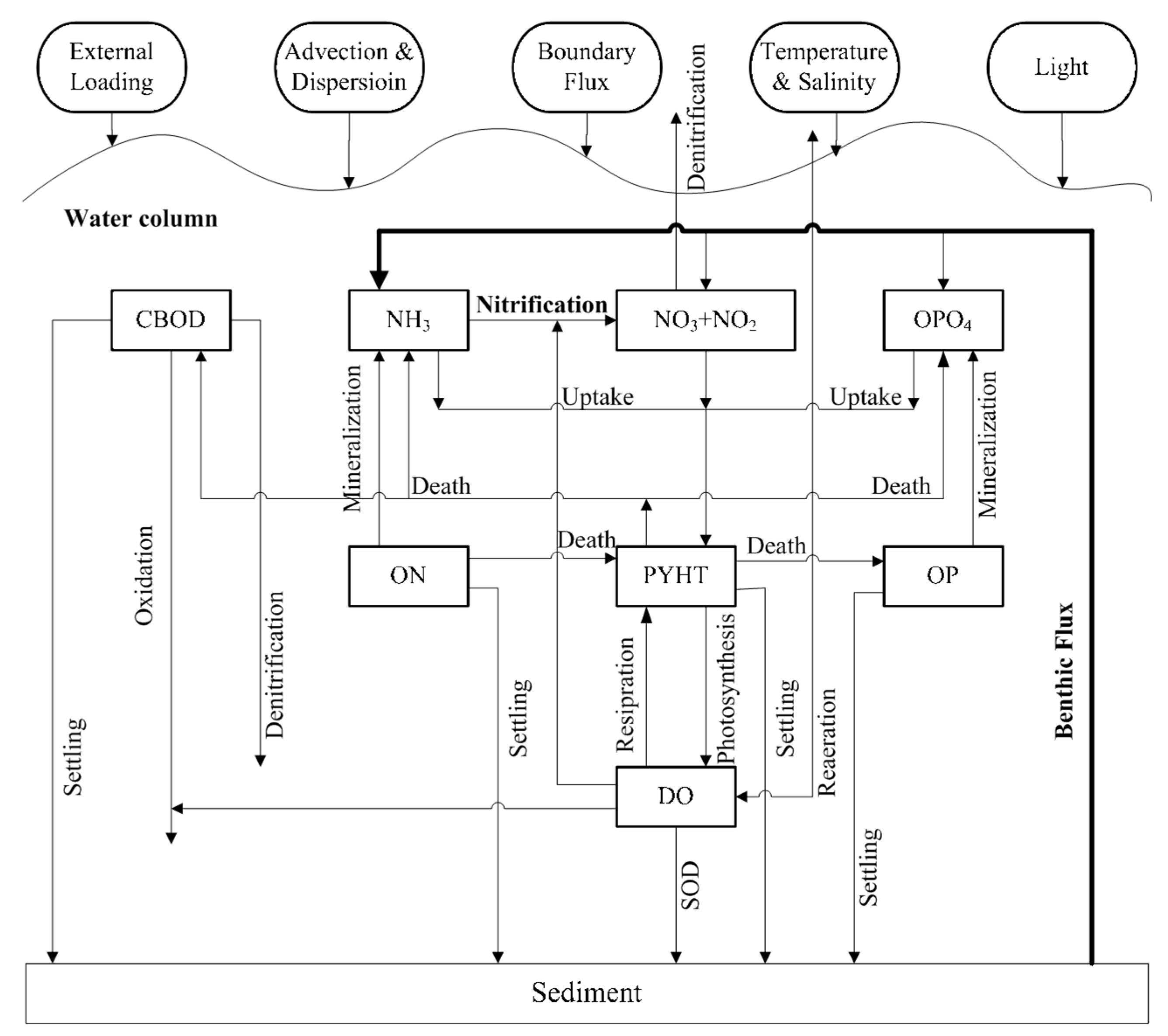
3.2. Water Quality Model

The water quality model used in this study was based on a three-dimensional conventional water quality analysis simulation program called WASP5, originally developed by Ambrose et al. [53]. It constitutes a complicated system of four interacting parts: dissolved oxygen, nitrogen cycle, phosphorus cycle, and phytoplankton dynamics. Eight water quality components are included: dissolved oxygen (DO), phytoplankton as carbon (PHYT), carbonaceous biochemical oxygen demand (CBOD), ammonium nitrogen (NH₄), nitrate and nitrite nitrogen (NO₃), organic nitrogen (ON), ortho-phosphorus or inorganic phosphorus (OP), and organic phosphorus (OP). The conceptual framework for the water quality model is presented in Figure 2.

A mathematical formulation of the conservation of mass can be written as follows:

$$\frac{\partial C}{\partial t}+\frac{\partial (uC)}{\partial x}+\frac{\partial (vC)}{\partial y}+\frac{\partial (wC)}{\partial z}=\frac{\partial }{\partial x}(A_h\frac{\partial C}{\partial x})+\frac{\partial }{\partial y}(A_h\frac{\partial C}{\partial y})+\frac{\partial }{\partial z}(K_v\frac{\partial C}{\partial z})+S_e+S_i$$

(1)

where C is the concentration of water quality components; u, v, and w are the water velocity components corresponding to a Cartesian coordinate system (x, y, z); A_h and K_v are the coefficients of horizontal viscosity and vertical eddy diffusion, respectively; S_e is the time rate of external additional (withdrawal) across the boundaries; and S_i is the time rate of internal increase/decrease by biogeochemical reaction processes.

Equation (1) gives the distribution of each state variable using the physical parameters determined from the hydrodynamic model. The last two terms, S_e and S_i represent, respectively, the external and internal sources (or sinks), the latter being primarily due to biogeochemical processes.

The present model of DO includes the following processes: source from photosynthesis, reaeration through surface and external loading, and sinks due to decay of CBOD, nitrification, algae respiration, and SOD. The mathematical representation is:

$$S_i=-K_{c}CBOD-a_{no}\frac{K_{n23}{N}_2}{K_{h23}+N_2}\frac{DO}{DO+K_{nit}}+a_c{a}_{co}(PQ\cdot G-\frac{R}{RQ})Chl$$

(2)

$$S_e=(1-{\lambda }_1)K_r(D{O}_s-DO)-\frac{SOD}{\mathsf{\Delta }z}\frac{DO}{DO+K_{DO}}+\frac{WDO}{V}$$

(3)

where a_c = ratio of carbon to chlorophyll in phytoplankton (mg C/μg Chl); a_co = ratio of oxygen demand to organic carbon recycled = 2.67; a_no = ratio of oxygen consumed per unit of ammonia nitrogen nitrified = 4.57; CBOD = concentration of carbonaceous of biochemical oxygen demand (mg/L); Chl = concentration of chlorophyll a (μg/L); DO = concentration of dissolved oxygen (mg/L); DO_s = saturation concentration of DO (mg/L); G = growth rate of phytoplankton (1/day); K_c = first-order decay rate of CBOD (1/day); K_DO = half-saturation concentration for benthic flux of CBOD (mg/L); K_h23 = half-saturation concentration for nitrification (mg/L); K_n23 = nitrification rate of ammonia nitrogen to nitrite-nitrate nitrogen (mg/L/day); K_nit = half-saturation concentration for oxygen limitation of nitrification (mg/L); K_r = reaeration rate (1/day); N₂ = concentration of ammonia nitrogen; PQ = photosynthesis quotient (mole O₂/mole C); R = respiration rate of phytoplankton (1/day); RQ = respiration quotient (mole CO₂/mole O₂); V = layer volume (cm³); WDO = external loading of DO (mg/day) including point and nonpoint sources; ∆z = layer thickness (cm); and λ₁ = 0 for k = 1 (at top layer), λ₁ = 1 for 2 ≤ k ≤ N, and N is the number of layers.

The sediment oxygen demand (SOD) in Equation (3) is the rate of oxygen consumption exerted by the bottom sediment and the overlay water due to the respiration of the benthic biological communities and the biochemical degradation of organic matter. The SOD is a major component of the dissolved oxygen (DO) budget and a key parameter to be determined through the model validation in the water quality model.

According to previous study implemented by Chen et al. [54], the component of phytoplankton species in the Danshuei River estuary includes diatoms, green algae, and others; therefore, these three major species are taken into account in the model simulation.

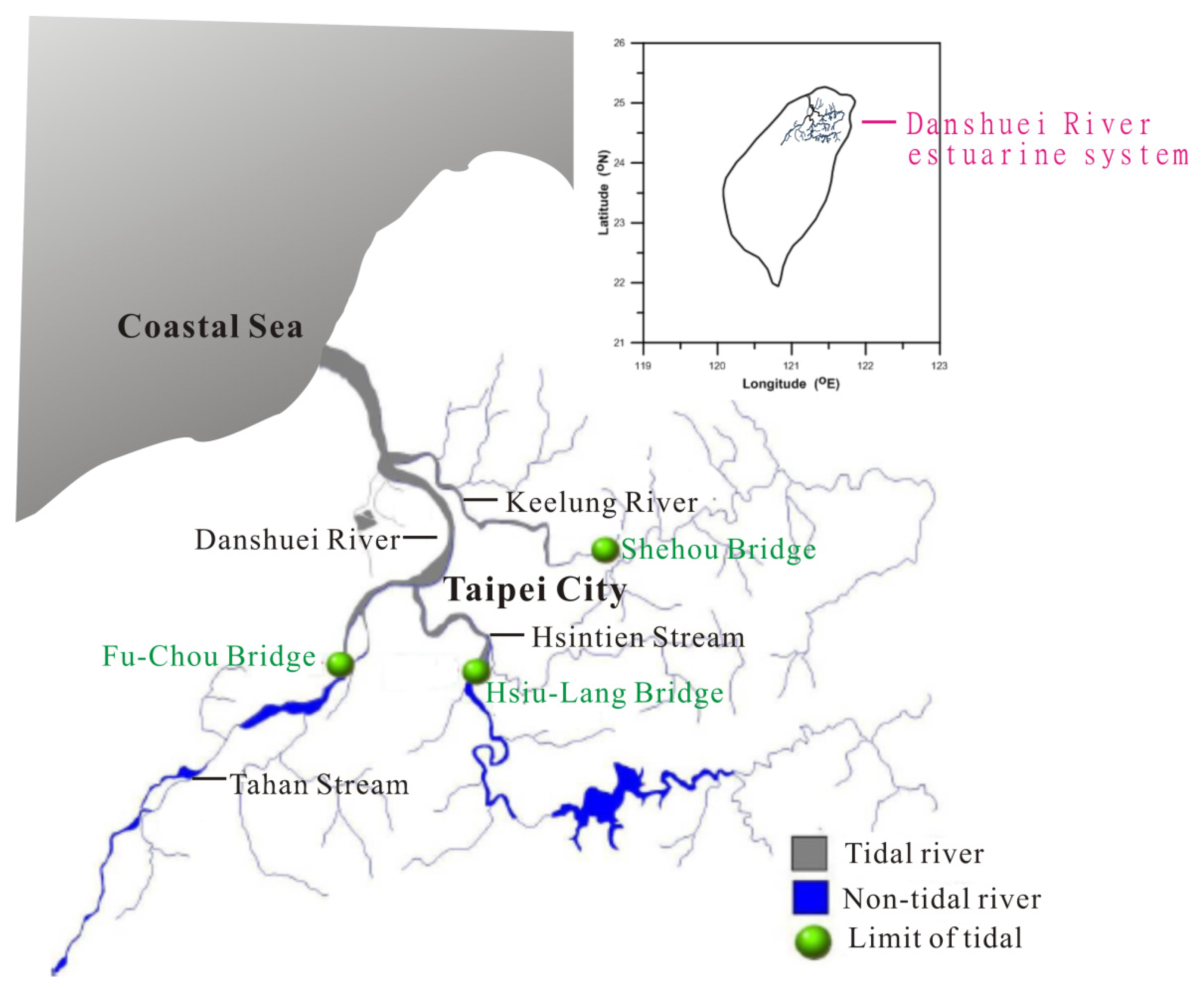
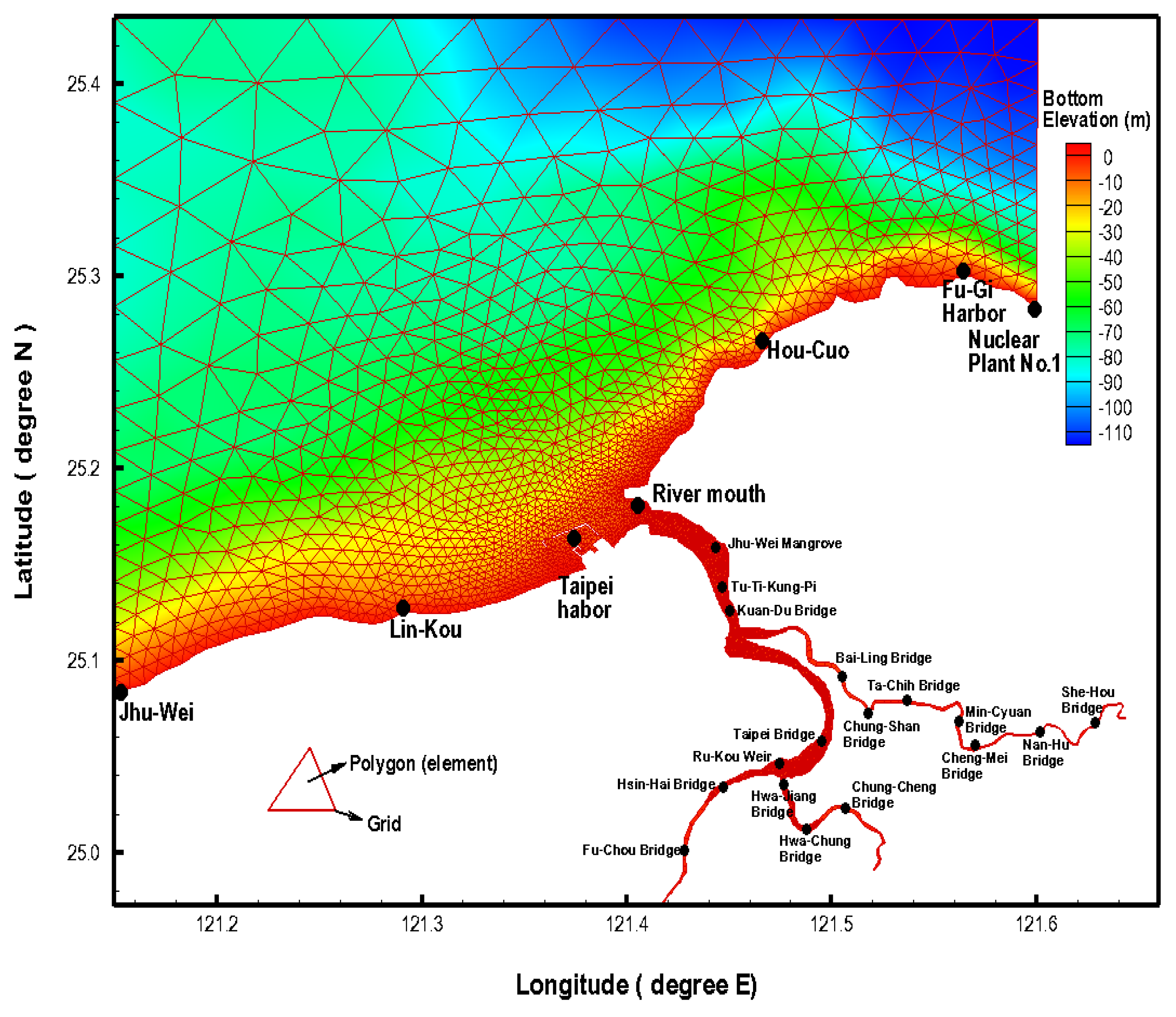
3.3. Model Schematization and Implementation

In the present study, the horizontal resolutions, 200 m × 200 m and 40 m × 40 m, of the bathymetric and topographical data in the Taiwan Strait and Danshuei-River estuarine system were obtained from the Ocean Data Bank and Water Resources Agency, Taiwan. The deepest point within the study area is 110 m (below the mean sea level) near the northeast corner of the computational domain (Figure 3). The model mesh for the Danshuei-River estuarine system and its adjacent coastal sea consists of 5119 elements (Figure 3). To meet the accuracy requirements, fine-grid resolution was used locally, and coarse resolution was implemented away from the region of interest. In this computational domain, the mesh size varied from 6000 m in the Taiwan Strait down to 40 m in the upper reach of Danshuei River estuary. The mesh size (40 m) used in the upper reach of Danshuei River estuary would be an appropriate resolution because the bathymetric and topographic data in 40 m × 40 m were only obtained.

In the vertical direction, ten z-levels and ten evenly spaced S-levels were specified at each horizontal grid, i.e., the thickness of the cell depended on the bottom elevation of each grid. The vertical resolutions in the coastal sea and Danshuei River estuary range from 10‒20 m and 0.015‒1.2 m, respectively. A 120-s time step was used in our simulations without any signs of numerical instability.

4. Model Validation

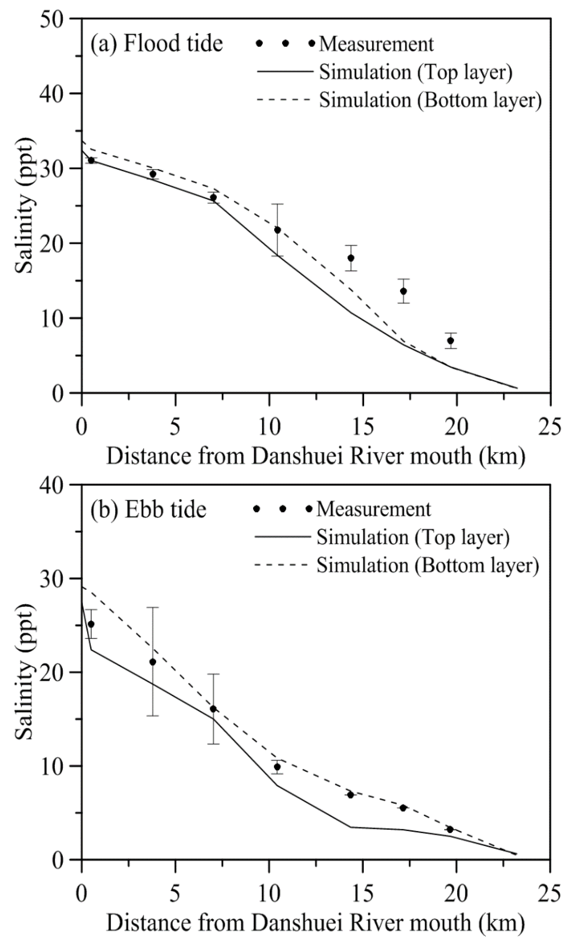
4.1. Salinity Distribution

Salinity distributions reflect the combined results of all processes, including density circulation and mixing processes. These processes in turn control the density circulation and modify the mixing processes [45]. In the present study, the salinity distribution along the Danshuei River-Tahan Stream collected by the Water Resources Agency, Taiwan, was used for model validation. Liu et al. [55] reported that a five-constituent tide (i.e., M₂, S₂, N₂, K₁, and O₁) is sufficient to represent the tidal components in the Taiwan Strait. The five-constituent tide was adopted in the model simulation as a forcing function at the coastal sea boundaries. The model was run for a two-year simulation. The salinity of the open boundaries in the coastal sea was set to 35 ppt. The upstream boundary conditions at the three tributaries (Tahan Stream, Hsintien Stream, and Keelung River) were specified with daily freshwater discharges; therefore, the salinity at the upstream boundaries was set to be 0 ppt.

The simulated salinity distribution compared favorably to the salinity measurements along the Danshuei River–Tahan Stream during the flood and ebb tides on 26 November 2010, shown in Figure 4. The measured salinity during the flood and ebb tides means that the salinity was measured at instantaneous flood and ebb tides. Note that the field data of salinity were measured 0.5 m below the water surface and then every 1.0 m below the water surface 0.5 m, and the simulated salinity was presented with the top layer and bottom layer. The measured salinity shown in Figure 4 presents the mean salinity in vertical direction plus/minus one standard deviation. The absolute mean error and root mean square error of the difference between the measured salinities and the computed salinity on 26 November 2010 are 2.71 ppt and 3.72 ppt, respectively, during the flood tide. The absolute mean error and root mean square error are 0.49 ppt and 0.67 ppt, respectively, during the ebb tide. It can be seen that the modeling performance for the ebb tide is better than that for the flood tide. This may be the reason that the higher horizontal eddy diffusion is calculated according to 2.5-equation closure model, resulting in salinity diffusion to the upstream region during the flood tide.

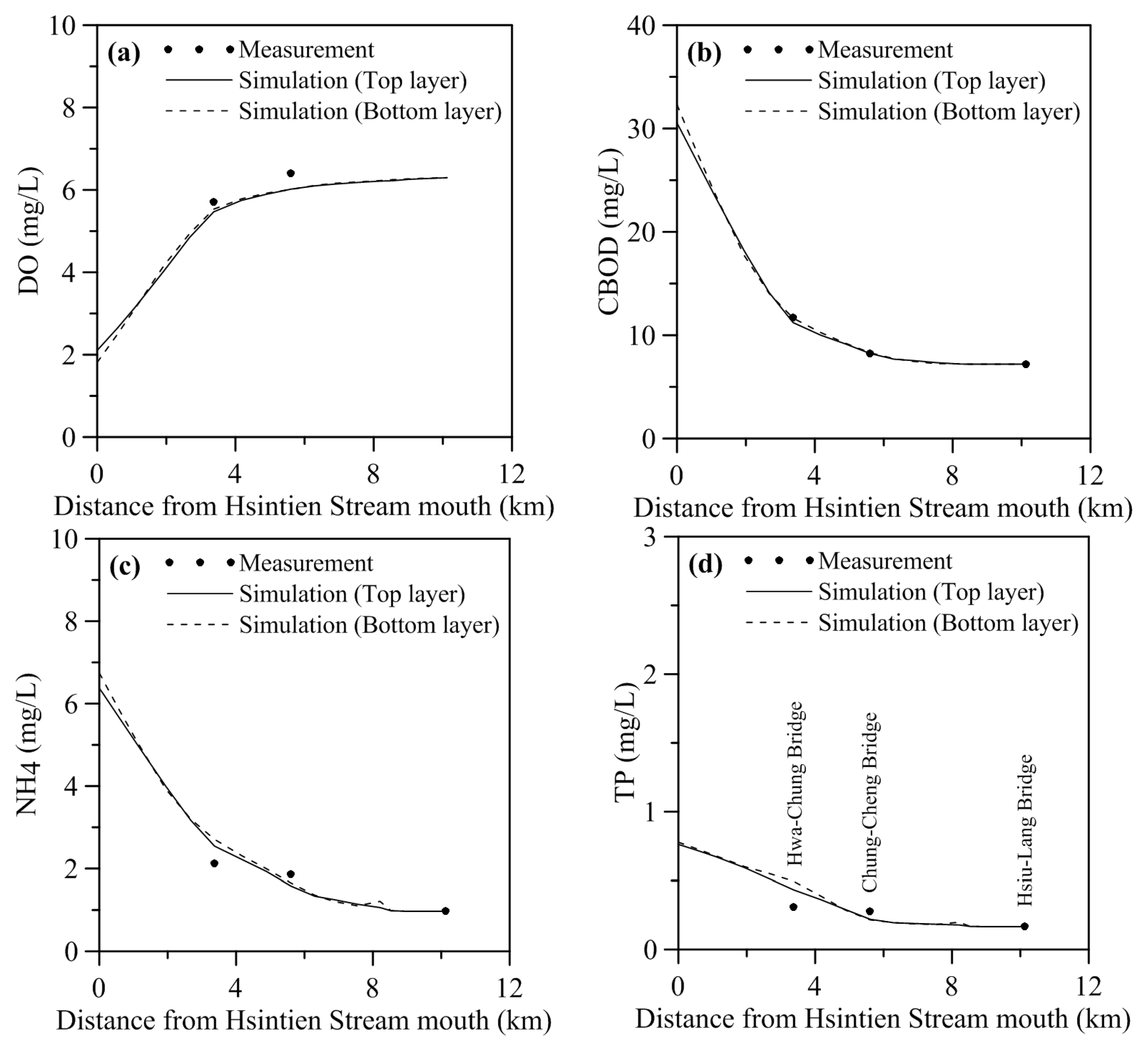
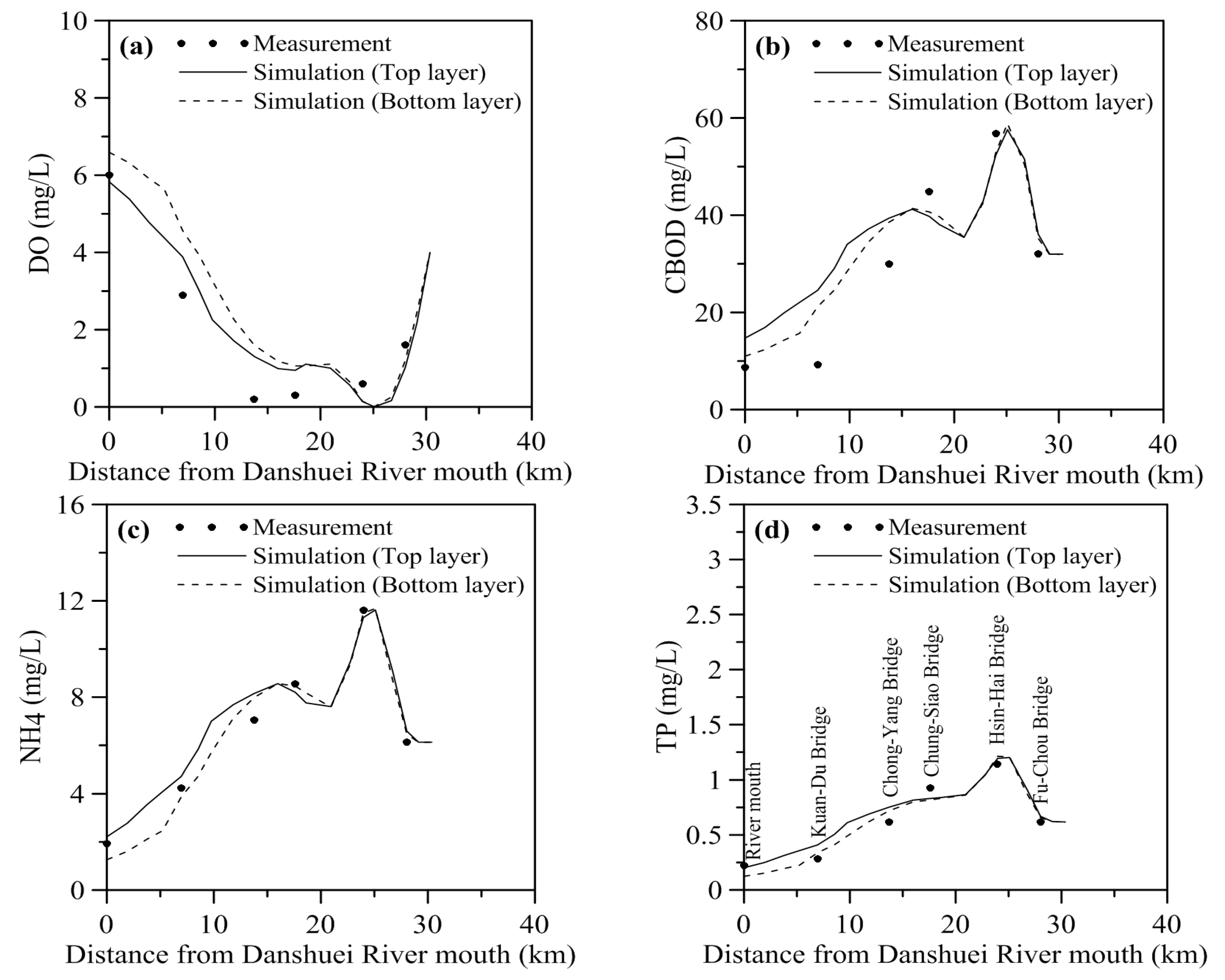
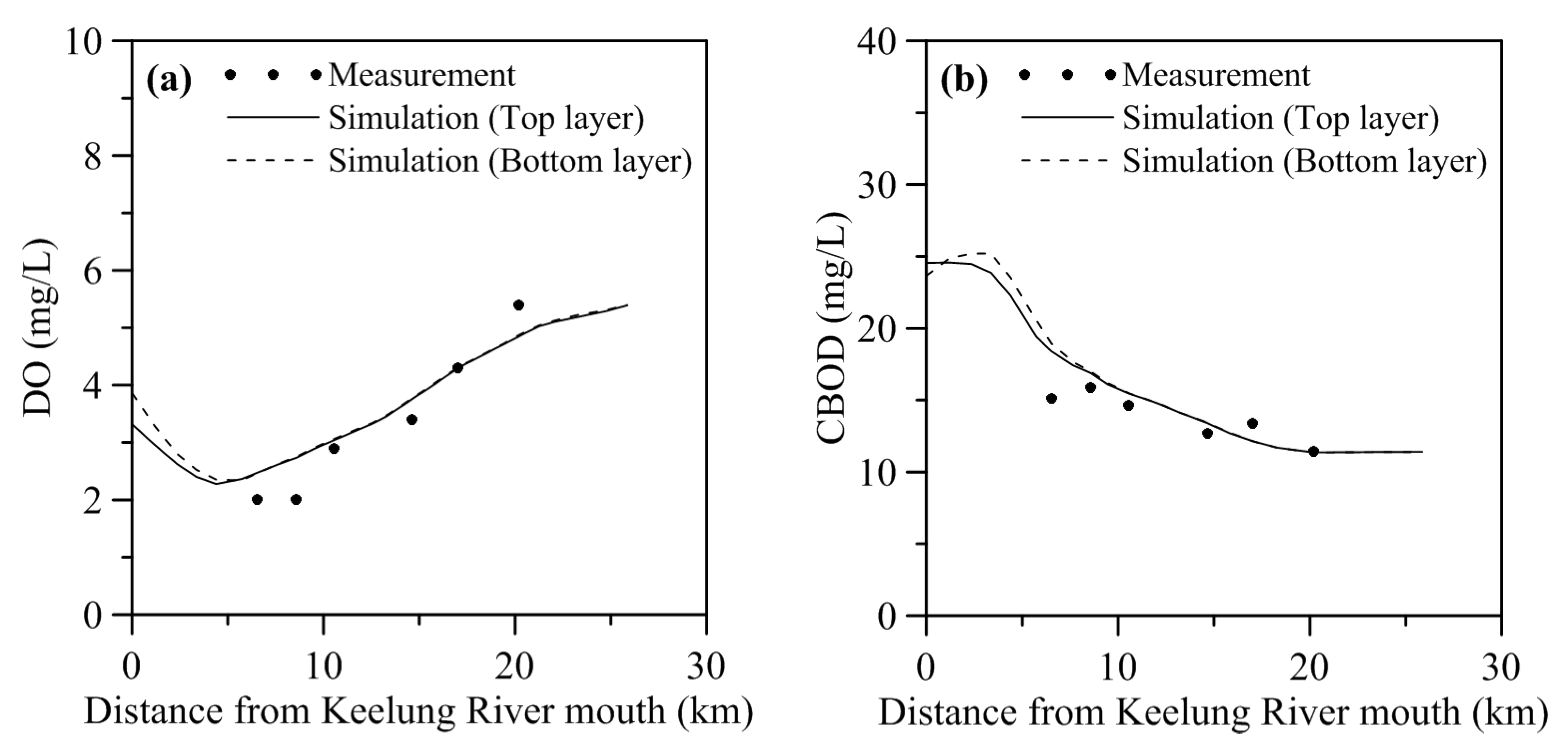
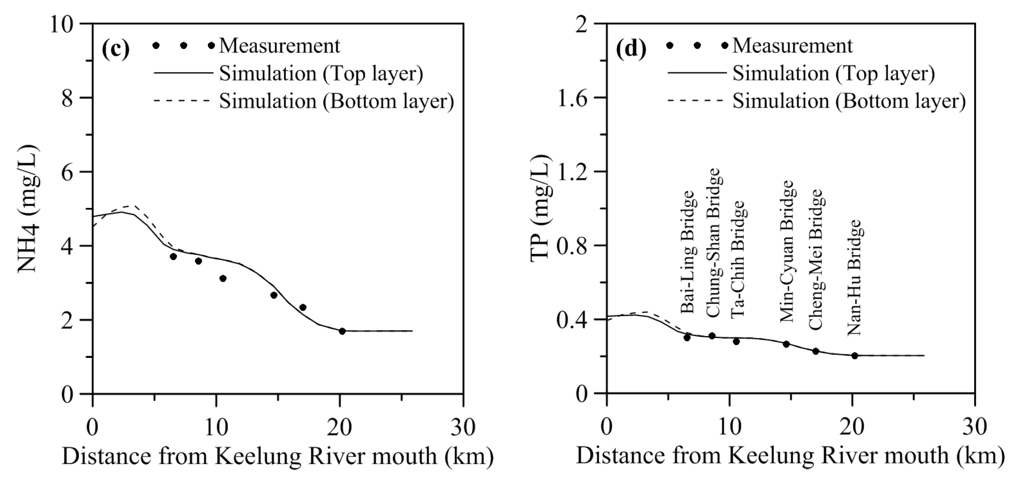
4.2. Water Quality Distribution

Chen et al. [56] implemented a comprehensive field sampling and lab analysis program for the Danshuei River to collect the data in 2009 and 2010. They found that adjacent to the metropolitan Taipei City, the spatial trend of the deteriorated water quality is mostly attributed to the wastewaters directly discharged into the river channels. Efforts were made successively to estimate the point source loadings by Montgomery Watson Harza (MWH) [57] adopted in the following water quality simulations. The freshwater discharges in 2010 and 2011 were adopted at the upstream boundaries at the Tahan Stream, the Hsintien Stream, and the Keelung River. The five-constituent tide used to generate the time-series tidal level was employed at the ocean boundaries. Concentrations of water quality state variables ammonium nitrogen, total nitrogen, total phosphorus, carbonaceous biochemical oxygen demand, dissolved oxygen, and chlorophyll a at the river boundaries and at the ocean boundaries were established based on the monthly measurement by the Taiwan Environmental Protection Administration (TEPA). The model was conducted with two-year simulation.

Eight measured datasets were collected on 1 March, 1 June, 3 September, 2 December in 2010, 3 March, 1 June, 5 September, and 1 December in 2011 and were used for model validation. The model parameters were initially estimated from the literature [58]. These were adjusted and tuned until a reasonable reproduction of field data at observation stations was obtained. The coefficients adopted for water quality simulations are listed in

Table 1. Coefficients used in the water quality model.

Coefficients	Value	Unit
Deoxygenation rate at 20 °C	0.16	day−1
Nitrification rate at 20 °C	0.13	day−1
Phytoplankton respiration rate at 20 °C	0.6	day−1
Denitrification rate at 20 °C	0.09	day−1
Organic nitrogen mineralization at 20 °C	0.075	day−1
Organic phosphorus mineralization at 20 °C	0.22	day−1
Optimum phytoplankton growth rate at 20 °C	2.5	day−1
Optimal temperature for growth of phytoplankton	16	°C
The morality rate of phytoplankton at 20 °C	0.003	day−1
Half-saturation constant for oxygen limitation of carbonaceous deoxygenation	0.5	mg O2 L−1
Half-saturation constant for oxygen limitation of nitrification	0.5	mg O2 L−1
Half-saturation constant for uptake of inorganic nitrogen	25	μg N L−1
Half-saturation constant for uptake of inorganic phosphorus	1	μg P L−1
Half-saturation constant for oxygen limitation of denitrification	0.1	mg O2 L−1
Half-saturation constant of phytoplankton limitation of phosphorus recycle	1	mg C L−1
Sediment oxygen demand at 20 °C	3.5	g/m2 day
Optimal solar radiation rate	250	langleys/day
Total daily solar radiation	300	langleys/day
Ratio of nitrogen to carbon in phytoplankton	0.25	mg N/mg C
Ratio of phosphorus to carbon in phytoplankton	0.025	mg P/mg C
Ratio of phytoplankton to carbon	0.04	mg Phyt/mg C
Organic carbon (as CBOD) decomposition rate at 20 °C	0.21	day−1
Anaerobic algae decomposition rate at 20 °C	0.01	day−1
Denitrification rate at 20 °C	0.01	day−1
Organic nitrogen decomposition rate at 20 °C	0.01	day−1
Organic phosphorus decomposition rate at 20 °C	0.01	day−1
Benthic NH4 flux	0.04	mg N day−1
Benthic NO3 flux	0.003	mg N day−1
Benthic PO4 flux	0.005	mg P day−1
Ratio of nitrogen to carbon	0.01	mg N/mg C
Ratio of phosphorus to carbon	0.01	mg P/mg C

. The longitudinal water quality distributions predicted by the water quality model on 3 March 2011 for the Danshuei River–Tahan Stream, the Hsintien Stream, and the Keelung River are shown in Figure 5, Figure 6 and Figure 7, respectively. Water quality distributions of the dissolved oxygen, carbonaceous biochemical oxygen demand, ammonium nitrogen, and total phosphorus concentrations at the top and bottom layers along the river channels are presented in the figures, together with the observations from monitoring stations. Both the model-predicted and observed dissolved oxygen concentrations along the Danshuei River–Tahan Stream show a decrease from the Danshuei River mouth to Hsin-Hai Bridge and an increase at the Fu-Chou Bridge (Figure 5a). In the lower estuary, the dissolved oxygen concentrations increase toward the river mouth as a result of seawater dilution. It also shows that quite low dissolved oxygen concentrations occur at the Chong-Yang Bridge, Chung-Siao Bridge, and Hsin-Hai Bridge. Carbonaceous biochemical oxygen demand, ammonium nitrogen, and total phosphorus all show the same spatial trends along the river channel from the Tahan Stream to the Danshuei River (Figure 5b‒d). The concentrations increase from the Danshuei River mouth to Hsin-Hai Bridge, reach a maximum at the Hsin-Hai Bridge, and then gradually decrease toward the Fu-Chou Bridge. The maximum concentrations of all three occur at the Hsin-Hai Bridge, resulting in low dissolved oxygen. The figure shows that the model generally captured the spatial trends of the observed longitudinal distributions.

The ratio of nitrogen to carbon in different water bodies has been documented in reports [59,60,61]. The ratio ranges from 0.02‒0.25 mg N/mg C. However, we set this ratio to 0.01 mg N/mg C in the model simulation, which is lower than the suggested value. This is the reason that the concentration of ammonium nitrogen (NH₄) in the Danshuei River estuarine system is quite high compared to other estuaries [10,42,62]. If we adopted the higher ratio of nitrogen to carbon in the model, the simulation results of CBOD would be too high and DO would be too low to compare with the measured data.

The longitudinal water quality distributions along the Hsintien Stream are illustrated in Figure 6. Both the observation data and model predictions show that the water quality conditions degrade as the river reach approaches the Hsintien Stream mouth, where it joins the main stream of the Danshuei River; the dissolved oxygen decreases, and the organic carbon, ammonium nitrogen and total phosphorus increase monotonically. The model faithfully represents the observed carbonaceous biochemical oxygen demand, ammonium nitrogen, and total phosphorus along the Hsintien Stream.

The longitudinal water quality distribution along the Keelung River (Figure 7) shows that significant pollution loadings were discharged into the river section around the Bai-Ling Bridge and the Chung-Shan Bridge, where the lowest dissolved oxygen in the Keelung River was observed. The model can realistically mimic the observed dissolved oxygen. The model was also revealed to match the observed carbonaceous biochemical oxygen demand, ammonium nitrogen, and total phosphorus very well along the Keelung River. Due to the page limitation, the statistical errors, including the absolute mean error and root mean square error on 2 December 2010, 3 March, 1 June, 5 September 2011 are shown only in

Table 2. Statistical error between simulated and measured water quality state variables on 2 December 2010.

Water Quality Variable	Danshuei River–Tahan Stream		Hsintien Stream		Keelung River
	AME (mg/L)	RMSE (mg/L)	AME (mg/L)	RMSE (mg/L)	AME (mg/L)	RMSE (mg/L)
Dissolved oxygen	0.63	0.88	2.17	3.47	0.91	0.98
Carbonaceous biochemical oxygen demand	2.21	2.79	1.79	2.29	2.02	2.51
Ammonium nitrogen	0.36	0.54	0.52	0.74	0.15	0.19
Total phosphorus	0.07	0.10	0.08	0.12	0.008	0.01

,

Table 3. Statistical error between simulated and measured water quality state variables on 3 March 2011.

Water Quality Variable	Danshuei River–Tahan Stream		Hsintien Stream		Keelung River
	AME (mg/L)	RMSE (mg/L)	AME (mg/L)	RMSE (mg/L)	AME (mg/L)	RMSE (mg/L)
Dissolved oxygen	0.74	0.85	0.86	1.18	0.38	0.45
Carbonaceous biochemical oxygen demand	6.56	7.5	0.11	0.16	1.25	1.67
Ammonium nitrogen	0.35	0.46	0.25	0.32	0.23	0.27
Total phosphorus	0.08	0.08	0.07	0.09	0.01	0.01

,

Table 4. Statistical error between simulated and measured water quality state variables on 1 June 2011.

Water Quality Variable	Danshuei River–Tahan Stream		Hsintien Stream		Keelung River
	AME (mg/L)	RMSE (mg/L)	AME (mg/L)	RMSE (mg/L)	AME (mg/L)	RMSE (mg/L)
Dissolved oxygen	0.83	0.97	0.29	0.44	0.68	0.76
Carbonaceous biochemical oxygen demand	2.48	2.84	2.23	2.85	1.60	1.86
Ammonium nitrogen	0.52	0.80	0.44	0.67	0.35	0.42
Total phosphorus	0.99	0.10	0.08	0.14	0.06	0.07

and

Table 5. Statistical error between simulated and measured water quality state variables on 5 September 2011.

Water Quality Variable	Danshuei River–Tahan Stream		Hsintien Stream		Keelung River
	AME (mg/L)	RMSE (mg/L)	AME (mg/L)	RMSE (mg/L)	AME (mg/L)	RMSE (mg/L)
Dissolved oxygen	1.41	1.65	0.67	0.83	1.04	1.19
Carbonaceous biochemical oxygen demand	1.10	1.32	006	0.07	0.80	0.91
Ammonium nitrogen	0.47	0.78	0.03	0.04	0.56	0.71
Total phosphorus	0.04	0.06	0.01	0.01	0.02	0.02

.

Note that AME = $\frac{1}{N}{\displaystyle \sum _{i=1}^N\left|{(C_p)}_i-{(C_o)}_i\right|},$ RMSE = $\sqrt{\frac{1}{N}{\displaystyle \sum _{i=1}^N{[{(C_p)}_i-{(C_o)}_i]}^2}},$ where C_p is the predicted water quality concentration; and C_o is the observed water quality concentration.

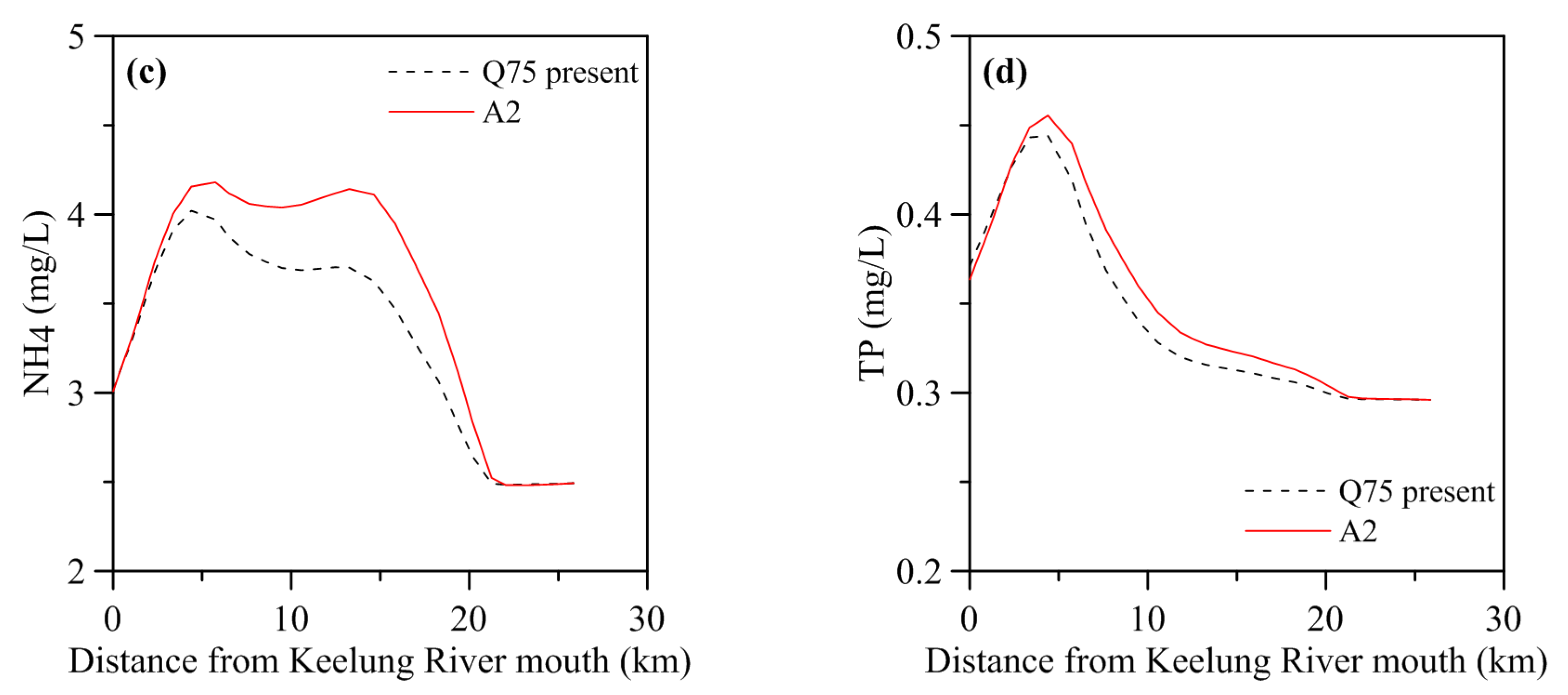
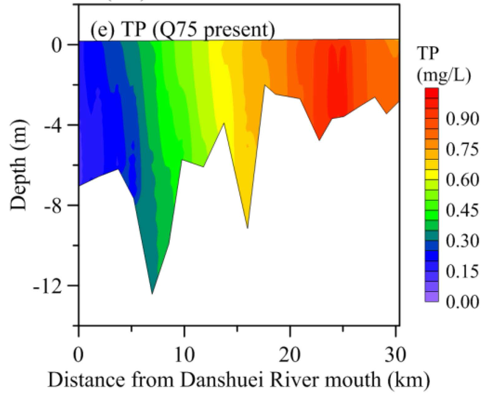
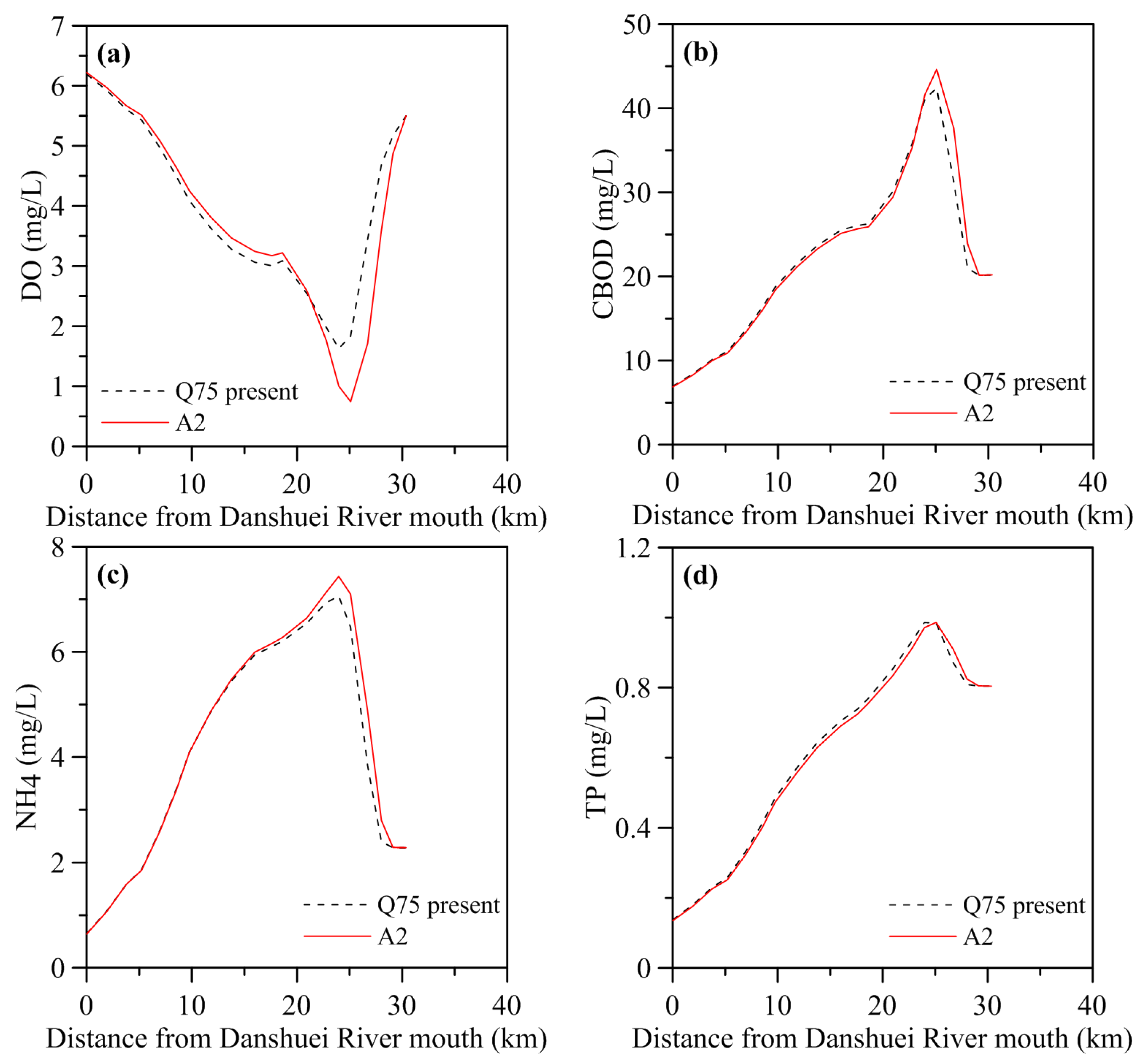
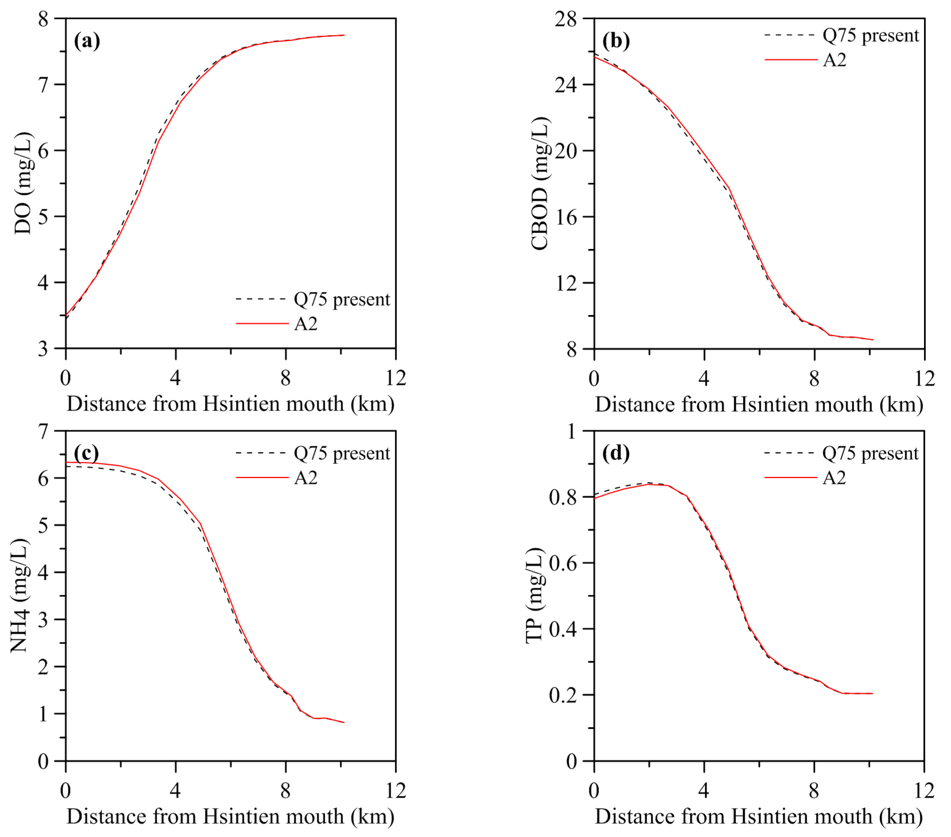
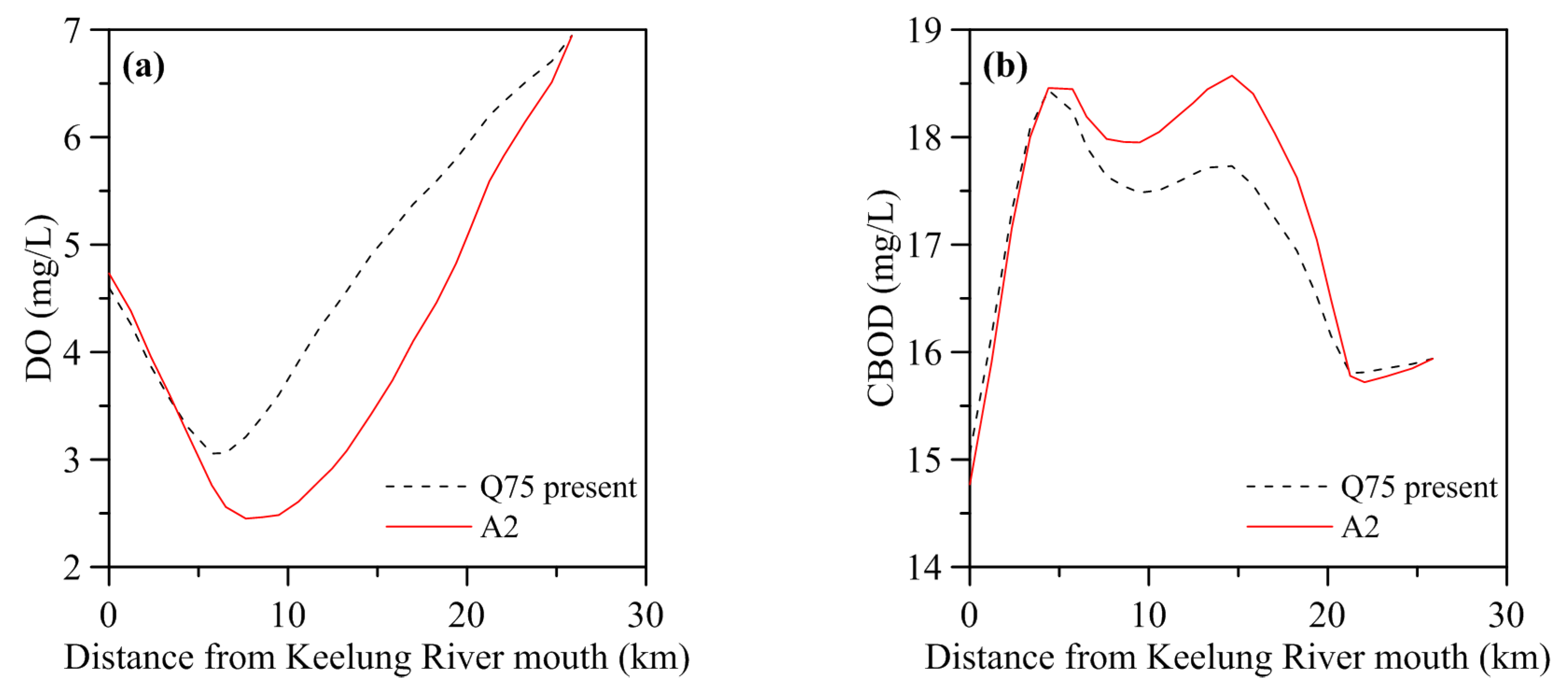
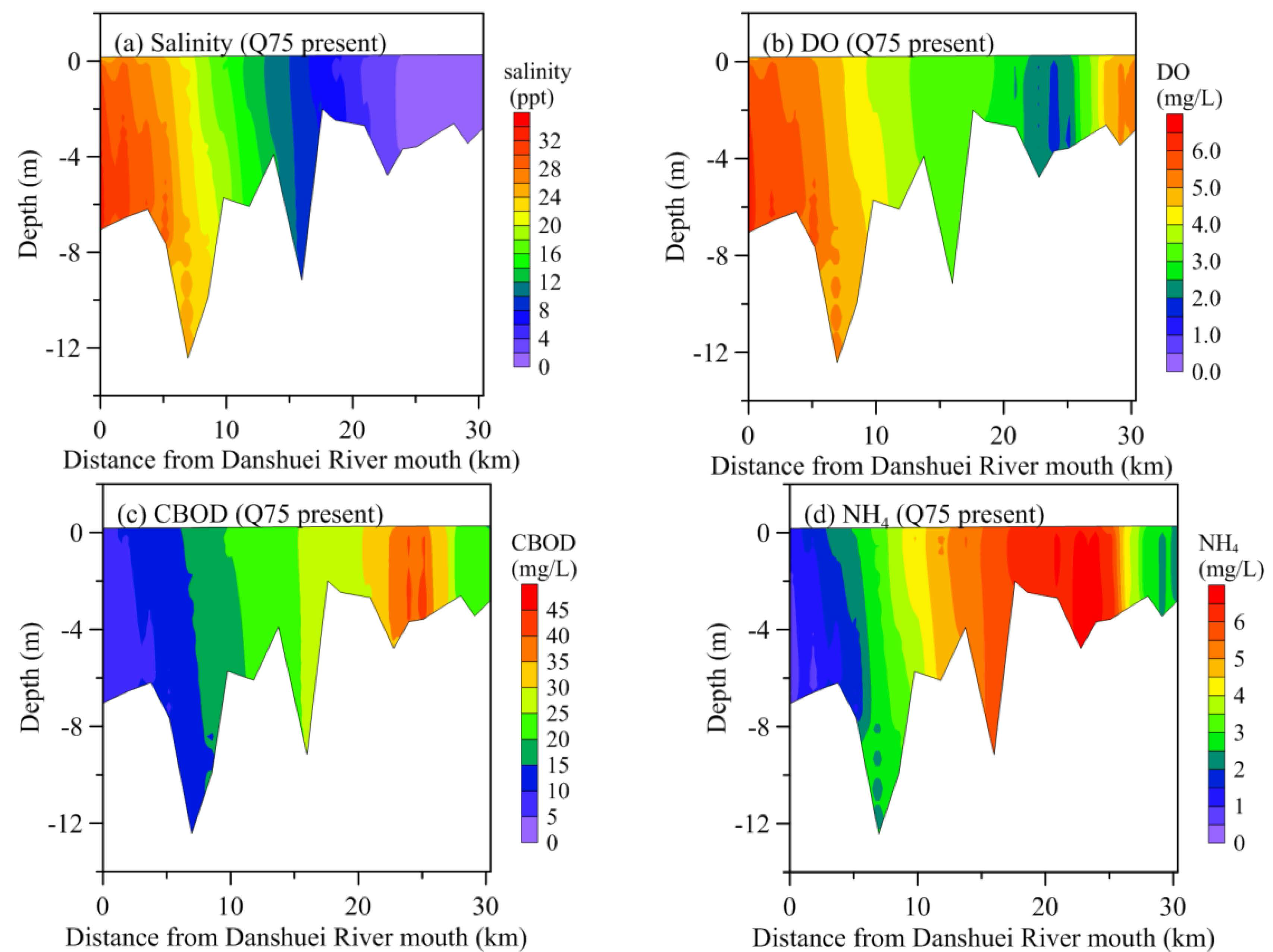
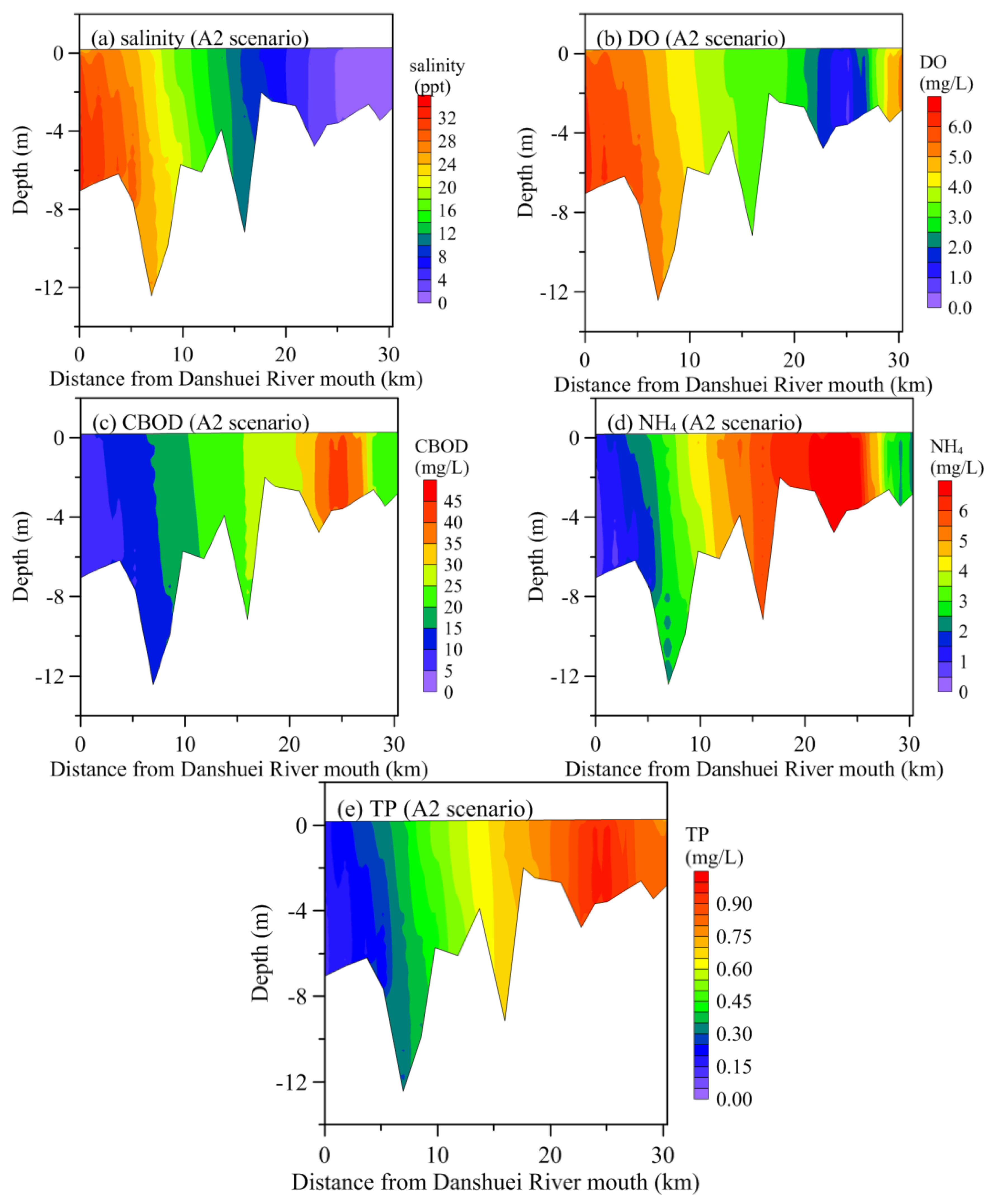
5. Model Project Responses to Climate Change Impact

The future climate scenarios frequently used in Taiwan have been based on the Intergovernmental Panel on Climate Change (IPCC) Special Report on Emissions Scenarios (SRES) A1B and A2 scenarios. The Water Resources Agency [58] projected the streamflow in the Danshuei River basin due to the climate change scenarios in year 2039 (i.e., short term). The projected results in streamflow during the dry seasons based on different scenarios are summarized in

Table 6. The streamflows for the present condition and under climate change scenarios during Q75 low flow.

River	Q75 Low Flow under Present Condition (m3/s)	Decreasing Rate under A2 Scenario (%)	Q75 Low Flow under A2 Scenario (m3/s)	Decreasing Rate under A1B Scenario (%)	Q75 Low Flow under A1B Scenario (m3/s)
Tahan Stream	3.36	45.54	1.83	19.05	2.72
Hsintien Stream	14.23	4.15	13.64	3.44	13.74
Keelung River	3.33	45.65	1.81	24.32	2.52

. These results indicate that the decreasing rates of streamflows in the Tahan Stream, the Hsintien Stream, and the Keelung River are 45.54%, 4.15%, and 45.65%, respectively, for the A2 scenarios, whereas they are 19.05%, 3.44%, and 24.32%, respectively, for the A1B scenario.

To perform the model prediction of the water quality in the estuarine system, the five-constituent tide at the ocean boundaries was used to force the model simulation. Concentrations of the water quality state variables ammonium nitrogen, total nitrogen, total phosphorus, carbonaceous biochemical oxygen demand, dissolved oxygen, and chlorophyll a at the river boundaries and at the ocean boundaries were established based on mean values calculated from the measured water quality data collected from 2003 to 2013 as observed by TEPA. The river discharges at the tidal limits of the three major tributaries—the Tahan Stream, the Hsintien Stream, and the Keelung River—were conducted using the Q75 low flow condition, where Q75 flow is the flow that is equaled or exceeded 75% of the time. The Q75 river flows at the upstream reaches of the Tahan Stream, the Hsintien Stream, and the Keelung River are 3.36, 14.23, and 3.33 m³/s, respectively, for the present condition. For the A2 and A1B scenarios, the Q75 river flows at the upstream reaches of the Tahan Stream, the Hsintien Stream, and the Keelung River are presented in Table 6.

The predicted water quality distribution for the present condition and the A2 climate change scenario under Q75 low flow along the Danshuei River to the Tahan Stream, the Hsintien Stream, and the Keelung River, respectively, is shown in Figure 8, Figure 9 and Figure 10. A comparison of the present condition with the A2 climate change scenario reveals that the dissolved oxygen concentration decreased by a maximum of 1.75 mg/L and that the carbonaceous biochemical oxygen demand, ammonium nitrogen, and total phosphorus increased by a maximum of 6.4, 1.1, and 0.04 mg/L, respectively, in the Danshuei River–Tahan Stream (Figure 8). The dissolved oxygen concentration decreased by a maximum of 0.15 mg/L, and the carbonaceous biochemical oxygen demand, ammonium nitrogen, and total phosphorus increased by a maximum of 0.33, 0.14, and 0.01 mg/L, respectively, in the Hsintien Stream (Figure 9). The dissolved oxygen concentration decreased by a maximum of 1.50 mg/L, and the carbonaceous biochemical oxygen demand, ammonium nitrogen, and total phosphorus increased by a maximum of 0.85, 0.48, and 0.03 mg/L, respectively, in the Keelung River (Figure 10). We found that the dissolved oxygen concentration was lower than 2 mg/L in the Danshuei River-Tahan Stream and did not meet the minimum requirement of TEPA. The maximum rate of dissolved oxygen, carbonaceous biochemical oxygen demand, ammonium nitrogen, and total phosphorus under climate change scenarios A2 and A1B is summarized in

Table 7. Maximum rate of water quality state variables under climate change scenarios A2 and A1B.

River	Maximum Rate under Climate Change A2 Scenario				Maximum Rate under Climate Change A1B Scenario
	DO (%)	CBOD (%)	NH4 (%)	TP (%)	DO (%)	CBOD (%)	NH4 (%)	TP (%)
Danshuei River–Tahan Stream	−59.4	20.46	26.9	4.4	−25.8	7.5	9.8	1.8
Hsintien Stream	−2.0	1.9	3.8	1.7	−1.9	1.6	3.0	1.6
Keelung River	−33.7	4.9	13.8	6.2	−14.5	2.3	6.2	3.3

Note: minus and plus represent a decrease and increase, respectively.

. The maximum rate refers to the maximum values determined by the formula represented by $\frac{C_p-C_c}{C_p}\times 100\%$, where C_p is the water quality concentration at the present time and C_c is the water quality concentration under climate change.

The vertical distributions of monthly (in August) average salinity, dissolved oxygen, carbonaceous biochemical oxygen demand, ammonium nitrogen, and total phosphorus in the Danshuei River-Tahan Stream under the present condition and A2 scenario, respectively, are shown in Figure 11 and Figure 12. It can be seen that the limit of salt water intrusion for the A2 scenario (Figure 12a) moves further upriver compared with the present condition (Figure 11a). The limit of salt water intrusion for the present condition, A2 scenario, and A1B scenario in the Danshuei River-Tahan Stream, the Hsintien Stream, and the Keelung River is illustrated in

Table 8. The limit of salt water intrusion in the Danshuei River estuarine system under different scenarios.

River	Present Condition (km)	A2 Scenario (km)	A1B Scenario (km)
Danshuei River–Tahan Stream	24.67	26.19	25.24
Hsintien Stream	3.06	3.31	3.20
Keelung River	11.29	12.62	11.80

. The differences in the limit of salt water intrusion between the A2 scenario and present condition are 1.52 km, 0.25 km, and 1.33 km, respectively, in the Danshuei River-Tahan Stream, the Hsintien Stream, and the Keelung River. According to Figure 11a and Figure 12a, we can observe the vertical stratification in salinity exhibited in the lower Danshuei River estuary. The dissolved oxygen concentration for the A2 scenario (Figure 12b) in an estuarine system decreases compared to the present condition (Figure 11b), while the concentrations of carbonaceous biochemical oxygen demand, ammonium nitrogen, and total phosphorus (Figure 12c‒e) increase (Figure 11c‒e). No significant vertical stratification in water quality was found in the Danshuei River estuary.

6. Discussion

Water quality studies utilizing a coupled hydrodynamic and water quality model tend to contain some limitations and assumptions. These limitations and assumptions exist in both the data and model. The major data used in this study were climate change scenarios. The climate change scenarios (i.e., A1B and A2) used in this study were obtained from the Water Resources Agency, Taiwan, which projected the streamflow during dry seasons in the Danshuei River basin. We know that climate change is a non-stationary and dynamic problem; however, the streamflow projected from the climate change model and used in this study is a steady-state condition. This could lead to bias in future streamflow estimates that result in more uncertainty in the modeling results of water quality.

As mentioned in the Section “Water Quality Model”, there are many parameters in the water quality model. The model was validated with two-year measured data. The model parameters after validation are kept for modeling future conditions without adjustment under future scenarios. However, future climate change might change the parameters. All of these parameters might reduce the accuracy of the modeling results. Nevertheless, after considering the aforementioned limitations and assumptions, the modeling results of water quality are relevant and reliable under the current climate change scenarios. The approaches are useful for assessing the impact of climate change on estuarine water quality.

Some literature has stated that climate change causes the degradation of water quality. For example, Tung et al. [59] evaluated the effects of climate change on sustainable water quality management and proposed a systematic assessment procedure including a weather generation model, the streamflow component of GWLF, QUAL2E, and an optimization model. Their studies indicated that streamflows may likely increase in humid seasons and decrease in arid seasons. The reduction of streamflow in arid seasons might further degrade water quality and assimilation capacity. Our study also demonstrated that the dissolved oxygen would decrease as a result of climate change, which reduces the streamflow during dry seasons. Wetz and Yoskowitz [27] reported that drought coupled with burgeoning population growth in coastal watersheds places a serve strain on freshwater supplies and greatly reduces freshwater inflows to estuaries, especially when coincident with seasonal peaks in human freshwater demand. Freshwater contains nutrients and organic matter that upon delivery to the coastal zone, fuels the rich productivity of coastal ecosystems and shapes critical fish habitats through its effects on salinity gradients and stratification. Low freshwater inflow events have the potential to significantly alter the water quality and ecosystem structure. In this study, we found that the dissolved oxygen would decrease and nutrients would increase for the low flow condition as a result of climate change. The decreased dissolved oxygen would result in malodor, fish mortality, and microbial proliferation, which causes the issue of public health.

In future research, future climate scenarios will be performed with a global climate model (GCM model) combined with a rainfall-runoff model to project time-series streamflow, which can be incorporated into the hydrodynamic and water quality model. The impact of sea-level rise on the estuarine water quality can be investigated. A long-term early warning system triggering proper adaptations to reduce climate change effects can also be studied.

7. Conclusions

A coupled three-dimensional hydrodynamic water quality model was applied to predict the water quality conditions in the Danshuei River estuarine system due to the projected effects of climate change. The model was validated against salinity distribution and water quality state variables including dissolved oxygen, carbonaceous biochemical oxygen demand, ammonium nitrogen, and total phosphorus. The simulated results using the three-dimensional hydrodynamic water quality model revealed that the computed salinity and water quality state variables well reproduced the observed data. The overall performance of the model is in qualitative agreement with the available field data.

The validated model was then used to assess the effects of climate change on water quality in the Danshuei River estuarine system during the low flow condition. Two climate change scenarios, A2 and A1B, were considered for model simulation. The simulated results indicated that the dissolved oxygen concentration has significantly decreased and the concentrations of carbonaceous biochemical oxygen demand, ammonium nitrogen, and total phosphorus have obviously increased because of climate change. Moreover, the dissolved oxygen concentration would be lower than 2 mg/L in the main stream of the Danshuei River estuary and would fail to meet the minimum requirement of TEPA. The deleterious water quality would produce other issues related to human pathogens and public health.

The simulated results may vary depending on the estuarine system, climate scenario, water quality model, and parameters considered. Considering the limitations of this study, the results are valid only under current climate change scenarios in the study area. However, the results and methodologies in this study still have implications for future water quality management in the estuarine system for the study area and other regions facing similar stresses from climate change.

References

1. Hobbie, J.E. Estuarine Science—A Synthetic Approach to Research and Practice; Island Press: Washington, DC, USA, 2000. [Google Scholar]
2. Pendleton, L.H. The Economic and Market Value of Coasts and Estuaries: What’s at Stake; Restore America’s Estuaries: Arlington, VA, USA, 2008; p. 182. [Google Scholar]
3. Yoskowitz, D.W.; Santos, C.; Allee, B.; Carollo, C.; Henderson, J.; Jordan, S.; Ritchie, J. Ecosystem Services in the Gulf of Mexico. In Proceedings of the Gulf of Mexico Ecosystem Services Workshop, Bay St. Louis, MS, USA, 16–18 June 2010; Harte Research Institute for Gulf of Mexico Studies: Corpus Christi, TX, USA, 2010; p. 16. [Google Scholar]
4. Skerratt, J.; Wild-Allen, K.; Rizwi, F.; Whitehead, J.; Coughanowr, C. Use of a high resolution 3D fully coupled hydrodynamic, sediment and biogeochemical model to understand estuarine nutrient dynamics under various water quality scenarios. Ocean Coast. Manag. 2013, 83, 52–66. [Google Scholar] [CrossRef]
5. Yoskowitz, D.W.; Werner, S.R.; Carollo, C.; Santos, C.; Washburn, T.; Isaksen, G.H. Gulf of Mexico offshore ecosystem services: Relative evaluation by stakeholders. Mar. Policy 2015, in press. [Google Scholar] [CrossRef]
6. Lee, R.W. Research of Construct Wetland Environment Model for Guandu Natural Park. Master’s Thesis, National Taiwan Ocean University, Keelung, Taiwan, 2012. [Google Scholar]
7. Daily, G.C. Introduction: What are Ecosystem Services? Nature’s Services: Societal Dependence on Natural Ecosystems; Island Press: Washington, DC, USA, 1997. [Google Scholar]
8. Chau, K.W. An unsteady three-dimensional eutrophication model in Tolo harbour, Hong Kong. Mar. Pollut. Bull. 2005, 51, 1078–1084. [Google Scholar] [CrossRef] [PubMed]
9. McGlathery, K.J.; Sundback, K.; Anderson, I.C. Eutrophication in shallow coastal bay and lagoons: The role of plants in the coastal filter. Mar. Ecol. Prog. Ser. 2007, 348, 1–18. [Google Scholar] [CrossRef]
10. Wild-Allen, K.; Skerratt, J.; Whitehead, J.; Rizwi, F.; Parslow, J. Mechanisms driving estuarine water quality: A 3D biogeochemical model for informed management. Estuar. Coast. Shelf Sci. 2013, 135, 33–45. [Google Scholar] [CrossRef]
11. Kennish, M.J. Environmental threats and environmental future of estuaries. Environ. Conserv. 2002, 29, 78–107. [Google Scholar] [CrossRef]
12. Paerl, H.W.; Valdes, L.M.; Peierls, B.L.; Adolf, J.E.; Harding, L.W. Anthropogenic and climatic influences on the eutrophication of large estuarine ecosystem. Limnol. Oceanogr. 2006, 51, 448–462. [Google Scholar] [CrossRef]
13. Rabalais, N.N.; Turner, R.E.; Diaz, R.J.; Justic, D. Global change and eutrophication of coastal waters. ICES J. Mar. Sci. 2009, 66, 1528–1537. [Google Scholar] [CrossRef]
14. McKibben, S.M.; Watkins-Brandt, K.S.; Wood, A.M.; Hunter, M.; Forster, Z.; Hopkins, A.; Du, X.; Eberhart, B.T.; Peterson, W.T.; White, A.E. Monitoring Oregon coastal harmful algae: Observations and implications for a harmful algal bloom-monitoring project. Harmful Algae 2015, 50, 32–44. [Google Scholar] [CrossRef]
15. Stone, M.C.; Hotchkiss, R.H.; Hubbard, C.M.; Fontaine, T.A.; Mearns, L.O.; Arnold, J.G. Impacts of climate change on Missouri River Basin water yield. J. Am. Water Resour. Assoc. 2001, 37, 1119–1129. [Google Scholar] [CrossRef]
16. Chang, H.; Knight, C.G.; Staneva, M.P.; Kostov, D. Water resource impacts of climate change in southwestern Bulgaria. Geojournal 2002, 57, 159–168. [Google Scholar] [CrossRef]
17. Moss, R.H.; Edmonds, J.A.; Hibbard, K.A.; Manning, M.R.; Ross, S.K.; Van Vuuren, D.P.; Carter, T.R.; Emori, S.; Kainuma, M.; Kram, T.; et al. The next generation of scenarios for climate change research and assessment. Nature 2010, 463, 747–756. [Google Scholar] [CrossRef] [PubMed]
18. Trenberth, K.E. Framing the way to relate climate extremes to chimate change. Clim. Change 2012, 115, 283–290. [Google Scholar] [CrossRef]
19. Feng, S.; Hu, Q.; Hung, W.; Ho, C.H.; Li, R.; Tang, Z. Projected climate regime shift under future global warming from multi-model, multi-scenario CMIP5 simulations. Glob. Planet Change 2014, 112, 41–52. [Google Scholar] [CrossRef]
20. Xin, X.; Zhang, L.; Zhang, J.; Wu, T.; Fang, Y. Climate change projection over East Asia with BCC_CSM1.1 climate model under RCP scenarios. J. Meteorl. Soc. Jpn. 2013, 91, 413–429. [Google Scholar] [CrossRef]
21. Braks, M.; van Ginkel, R.; Wint, W.; Sedda, L.; Sprong, H. Climate change and public health policy: Translating the science. Int. J. Environ. Res. Public Health 2014, 11, 13–29. [Google Scholar] [CrossRef] [PubMed]
22. Kendrovski, V.; Spasenovska, M.; Menne, B. The public health impacts of climate change in the former Yugoslav Republic of Mecedonia. Int. J. Environ. Res. Public Health 2014, 11, 5975–5988. [Google Scholar] [CrossRef] [PubMed]
23. Petkova, E.P.; Ebi, K.L.; Culp, D.; Redlener, I. Climate change and health on the U.S. Gulf Coast: Public health adaption is needed to address future risks. Int. J. Environ. Res. Public Health 2015, 12, 9342–9356. [Google Scholar] [CrossRef] [PubMed]
24. Luber, G.; Prudent, N. Climate change and human health. Trans. Am. Clin. Climatol. Assoc. 2009, 120, 113–117. [Google Scholar] [PubMed]
25. Whitehead, P.; Wade, A.; Butterfield, D. Potential impacts of climate change on water quality and ecology in six UK rivers. Hydrol. Res. 2009, 40, 113–122. [Google Scholar] [CrossRef]
26. Wu, Y.; Liu, S.; Gallant, A.L. Predicting impacts of increased CO2 and climate change on the water cycle and water quality in the semiarid James River Basin of the Midwestern USA. Sci. Total Environ. 2012, 430, 150–160. [Google Scholar] [CrossRef] [PubMed]
27. Wetz, M.S.; Yoskowitz, D.W. An “extreme” future for estuaries? Effects of extreme climate events on estuarine water quality and ecology. Mar. Pollut. Bull. 2013, 69, 7–18. [Google Scholar] [CrossRef] [PubMed]
28. Middelkoop, H.; Daamen, K.; Gellens, D.; Grabs, W.; Kwadijk, J.C.J.; Lang, H.; Parmet, B.W.; Schadler, B.; Schulla, J.; Wilke, K. Impact of climate change on hydrological regimes and water resources management in the Rhine Basin. Clim. Change 2001, 49, 105–128. [Google Scholar] [CrossRef]
29. Ducharne, A.; Baubion, C.; Beaudoin, N.; Benoit, M.; Billen, G.; Brisson, N.; Garnier, J.; Kieken, H.; Lebonvallet, S.; Ledoux, E.; et al. Long term prospective of the Seine River system: Confronting climate and direct anthropogenic changes. Sci. Total Environ. 2007, 375, 292–311. [Google Scholar] [CrossRef] [PubMed]
30. Robins, P.E.; Skov, M.W.; Lewis, M.J.; Gimenez, L.; Davies, A.G.; Malham, S.K.; Neill, S.P.; McDonald, J.E.; Whitton, T.A.; Jackson, S.E.; et al. Impact of climate change on UK estuaries: A review of past trends and potential projections. Estuar. Coast. Shelf Sci. 2016, 169, 119–135. [Google Scholar] [CrossRef]
31. Garcia, A.; Juanes, J.A.; Alvarez, C.; Revilla, J.A.; Medina, R. Assessment of the response of a shallow macrotidal estuary to changes in hydrological and wastewater inputs through numerical modeling. Ecol. Model. 2010, 221, 1194–1208. [Google Scholar] [CrossRef]
32. Zhou, N.; Westrich, B.; Jiang, S.; Wang, Y. A coupling simulation based on hydrodynamics and water quality model of the Pearl River Delta, China. J. Hydrol. 2010, 396, 267–276. [Google Scholar] [CrossRef]
33. Piliwal, R.; Patra, R.R. Applicability of MIKE 21 to assess temporal and spatial variation in water quality of an estuary under the impact of effluent from an industrial estate. Water Sci. Technol. 2011, 63, 1932–1943. [Google Scholar] [CrossRef]
34. Long, T.Y.; Wu, L.; Meng, G.H.; Guo, W.H. Numerical simulation for impacts of hydrodynamic conditions on algae growth in Chongqing Section of Jialing River, China. Ecol. Model. 2011, 222, 112–119. [Google Scholar] [CrossRef]
35. Gao, G.; Falconer, R.A.; Lin, B. Modelling effects of a tidal barrage on water quality indicator distribution in the Severn Estuary. Front. Environ. Sci. Eng. 2013, 7, 211–218. [Google Scholar] [CrossRef]
36. Hanfeng, Y.E.; Guo, S.; Li, F.; Li, G. Water quality evaluation in tidal river reaches of Liaohe River estuary, China using a revised QUAL2K model. Chin. Geogr. Sci. 2013, 23, 301–311. [Google Scholar]
37. Sun, J.; Lin, B.; Jiang, G.; Li, K.; Tao, J. Modelling study on environmental indicators in an estuary. Proc. Inst. Civil Eng. Water Manag. 2014, 167, 141–151. [Google Scholar] [CrossRef]
38. Seo, D.; Song, Y. Application of three-dimensional hydrodynamics and water quality model of the Youngsan River, Korea. Desalin. Water Treat. 2015, 54, 3712–3720. [Google Scholar] [CrossRef]
39. Tu, J. Combined impact of climate and land use changes in streamflow and water quality in eastern Massachusetts, USA. J. Hydrol. 2009, 379, 268–293. [Google Scholar] [CrossRef]
40. Rehana, S.; Mujumdar, P.P. River water quality response under hypothetical climate change scenarios in Tunga-Bhadra river, India. Hydrol. Process. 2011, 25, 3372–3386. [Google Scholar] [CrossRef]
41. Luo, Y.; Ficklin, D.L.; Liu, X.; Zhang, M. Assessment of climate change impacts on hydrology and water quality with a watershed modeling approach. Sci. Total Environ. 2013, 450, 72–82. [Google Scholar] [CrossRef] [PubMed]
42. Wan, Y.; Ji, Z.G.; Shen, J.; Hu, G.; Sun, D. Three dimensional water quality modeling of a shallow subtropical estuary. Mar. Environ. Res. 2012, 82, 76–86. [Google Scholar] [CrossRef] [PubMed]
43. Cerco, C.F.; Noel, M.R. Twenty-year simulation of Chesapeake Bay water quality using the CE-QUAL-ICM eutrophication model. J. Am. Water Resour. Assoc. 2013, 49, 1119–1133. [Google Scholar] [CrossRef]
44. Li, K.; Zhang, L.; Li, Y.; Zhang, L.; Wang, X. A three-dimensional water quality model to determine the environmental capacity of nitrogen and phosphorus in Jiaozhou Bay, China. Mar. Pollut. Bull. 2015, 91, 306–316. [Google Scholar] [CrossRef] [PubMed]
45. Hsu, M.H.; Kuo, A.Y.; Kuo, J.T.; Liu, W.C. Procedure to calibrate and verify numerical models of estuarine hydrodynamics. J. Hydraul. Eng. 1999, 125, 166–182. [Google Scholar] [CrossRef]
46. Liu, W.C.; Chen, W.B.; Hsu, M.H. Influence of discharge reductions on salt water intrusion and residual circulation in Danshuei River Estuary. J. Mar. Sci. Technol. 2011, 19, 596–606. [Google Scholar]
47. Wang, C.F.; Hsu, M.H.; Kuo, A.Y. Residence time of Danshuei River estuary, Taiwan. Estuar. Coast. Shelf Sci. 2004, 60, 381–393. [Google Scholar] [CrossRef]
48. Liu, W.C.; Liu, S.Y.; Hsu, M.H.; Kuo, A.Y. Water quality modeling to determine minimum instream flow for fish survival in tidal rivers. J. Environ. Manag. 2005, 76, 293–308. [Google Scholar] [CrossRef] [PubMed]
49. Wang, C.F.; Hsu, M.H.; Liu, W.C.; Hwang, J.S.; Wu, J.T.; Kuo, A.Y. Simulation of water quality and plankton dynamics in the Danshuei River Estuary, Taiwan. J. Environ. Sci. Health A 2007, 42, 933–953. [Google Scholar] [CrossRef] [PubMed]
50. Zhang, Y.L.; Baptista, A.M. SELFE: A semi-implicit Eulerian-Lagrangian finite-element model for cross-scale ocean circulation. Ocean Model. 2008, 21, 71–96. [Google Scholar] [CrossRef]
51. Shchepetkin, A.F.; McWilliams, J.C. A method for computing horizontal pressure-gradient force in an oceanic model with a nonaligned vertical coordinate. J. Geophys. Res. 2003, 108. [Google Scholar] [CrossRef]
52. Umlauf, L.; Buchard, H. A generic length-scale equation for geophysical turbulence models. J. Mar. Res. 2003, 61, 235–265. [Google Scholar] [CrossRef]
53. Ambrose, R.B., Jr.; Wool, T.A.; Martin, J.L. The Water Quality Analysis Simulation Program, WASP5, Part A: Model Documentation; U.S. Environmental Protection Agency: Athens, GA, USA, 1993; p. 202.
54. Chen, W.B.; Liu, W.C.; Hsu, M.H. Water quality modeling in a tidal estuarine system using a three-dimensional model. Environ. Eng. Sci. 2011, 28, 443–459. [Google Scholar] [CrossRef]
55. Liu, W.C.; Chen, W.B.; Kuo, J.T. Modeling residence time response to freshwater discharge in a mesotidal estuary, Taiwan. J. Mar. Syst. 2008, 74, 295–314. [Google Scholar] [CrossRef]
56. Chen, C.H.; Lung, W.S.; Yang, C.H.; Lin, C.F. Spatially variable deoxygenation in the Danshui River: Improvement in model calibration. Water Environ. Res. 2013, 85, 2243–2253. [Google Scholar] [CrossRef] [PubMed]
57. Montgomery Watson Harza (MWH). Evaluation of Hydrodynamics and Water Quality Monitoring and Management in the Danshuei River Basin of New Taipei City; Report to New Taipei City Government; Montgomery Watson Harza (MWH): Broomfield, CO, USA, 2011. [Google Scholar]
58. Bowie, G.L.; Mills, W.B.; Porcella, D.B.; Campbell, J.R.; Pagenkopf, J.R.; Rupp, G.L.; Johnson, K.M.; Chan, P.W.H.; Gherini, S.A. Rates, Constants, and Kinetics Formulations in Surface Water Quality Modeling, 2nd ed.EPA/600/3–85/040; Environmental Research Laboratory, Office of Research and Development, U.S. Environmental Protection Agency: Athens, GA, USA, 1985; p. 455.
59. Gray, K.R.; Biddlestone, A.J. Composing-process parameters. Chem. Eng. 1973, 2, 71–76. [Google Scholar]
60. Meyers, P.A.; Ryoshi, I. Lacustrine organic goechemistry—An overview of indicators of organic matter sources and diagenesis in lake sediments. Org. Geochem. 1993, 20, 867–900. [Google Scholar] [CrossRef]
61. Emerson, S.; Hedges, J. Sediment diagenesis and benthic flux. In Treatise on Geochemistry, 2nd ed.; Henry, E., Heinrich, D.H., Karl, K.T., Eds.; Elsevier: Amsterdam, The Netherlands, 2013; pp. 293–319. [Google Scholar]
62. Kim, T.; Sheng, Y.P.; Park, K. Modeling water quality and hypoxia dynamics in Upper Charlotte Harbor, Florida, U.S.A. during 2000. Estuar. Coast. Shelf Sci. 2010, 90, 250–263. [Google Scholar] [CrossRef]
63. Water Resources Agency. Strengthening Sustainable Water Resources Utilization and Adaptive Capability to Climate Change; Final Report; Water Resources Agency: Nantun, Taiwan; Taichung, Taiwan, 2008. (In Chinese) [Google Scholar]
64. Tung, C.P.; Lee, T.C.; Liao, W.T.; Chen, Y.J. Climate change impact assessment for sustainable water quality management. Terr. Atmos. Ocean. Sci. 2012, 23, 565–576. [Google Scholar] [CrossRef]
Figure 1. Danshuei River estuarine system and watershed.
Water 08 00060 g001
Figure 2. Schematic of water quality model.
Water 08 00060 g002
Figure 3. The topography of the Danshuei River estuarine system and its adjacent coastal and unstructured grid for the computational domain.
Water 08 00060 g003
Figure 4. The comparison between the measured and simulated salinities along the Danshuei River–Tahan Stream on 26 November 2010 during (a) flood tide and (b) ebb tide.
Water 08 00060 g004
Figure 5. The comparison between the measured and simulated water quality distributions along the Danshuei River to the Tahan Stream on 3 March 2011 (a) DO; (b) CBOD; (c) NH4; and (d) TP.
Water 08 00060 g005
Figure 6. The comparison between the measured and simulated water quality distributions along the Hsintien Stream on 3 March 2011 (a) DO; (b) CBOD; (c) NH4; and (d) TP.
Water 08 00060 g006
Figure 7. The comparison between the measured and simulated water quality distributions along the Keelung River on 3 March 2011 (a) DO; (b) CBOD; (c) NH4; and (d) TP.
Water 08 00060 g007aWater 08 00060 g007b
Figure 8. Predicting water quality distributions for present and climate change (A2 scenario) conditions under Q75 low flow along the Danshuei River to the Tahan Stream (a) DO; (b) CBOD; (c) NH4; and (d) TP.
Water 08 00060 g008
Figure 9. Predicting water quality distributions for present and climate change (A2 scenario) conditions under Q75 low flow along the Hsintien Stream (a) DO; (b) CBOD; (c) NH4; and (d) TP.
Water 08 00060 g009
Figure 10. Predicting water quality distribution for present and climate change (A2 scenario) conditions under Q75 low flow along the Keelung River (a) DO; (b) CBOD; (c) NH4; and (d) TP.
Water 08 00060 g010aWater 08 00060 g010b
Figure 11. The vertical distribution of the monthly average water quality concentration in the Danshuei River to Tahan Stream under Q75 flow for the present condition (a) Salinity; (b) DO; (c) CBOD; (d) NH4; and (e) TP.
Water 08 00060 g011aWater 08 00060 g011b
Figure 12. The vertical distribution of the monthly average water quality concentration in the Danshuei River to Tahan Stream under Q75 flow for the A2 Scenario (a) Salinity; (b) DO; (c) CBOD; (d) NH4; and (e) TP.
Water 08 00060 g012