
Using a Geospatial Model to Relate Fluvial Geomorphology to Macroinvertebrate Habitat in a Prairie River—Part 1: Genus-Level Relationships with Geomorphic Typologies


Abstract
:1. Introduction
2. Methods
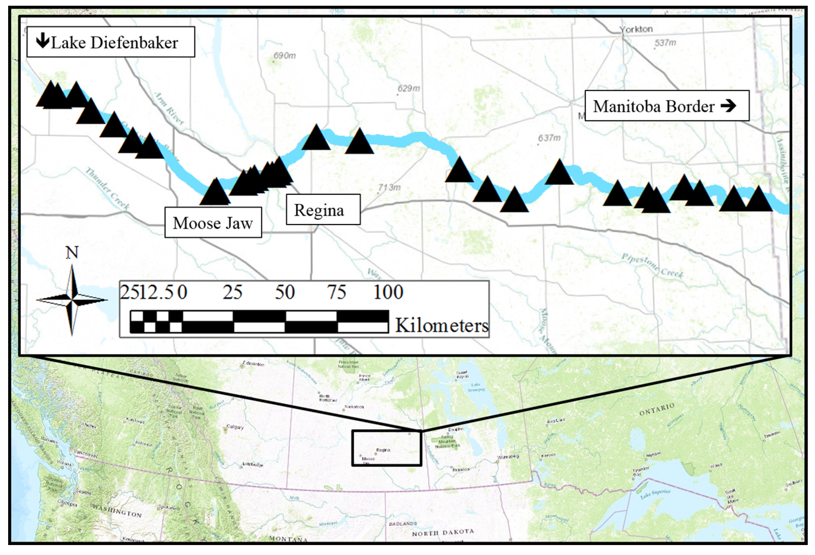
2.1. Study Site
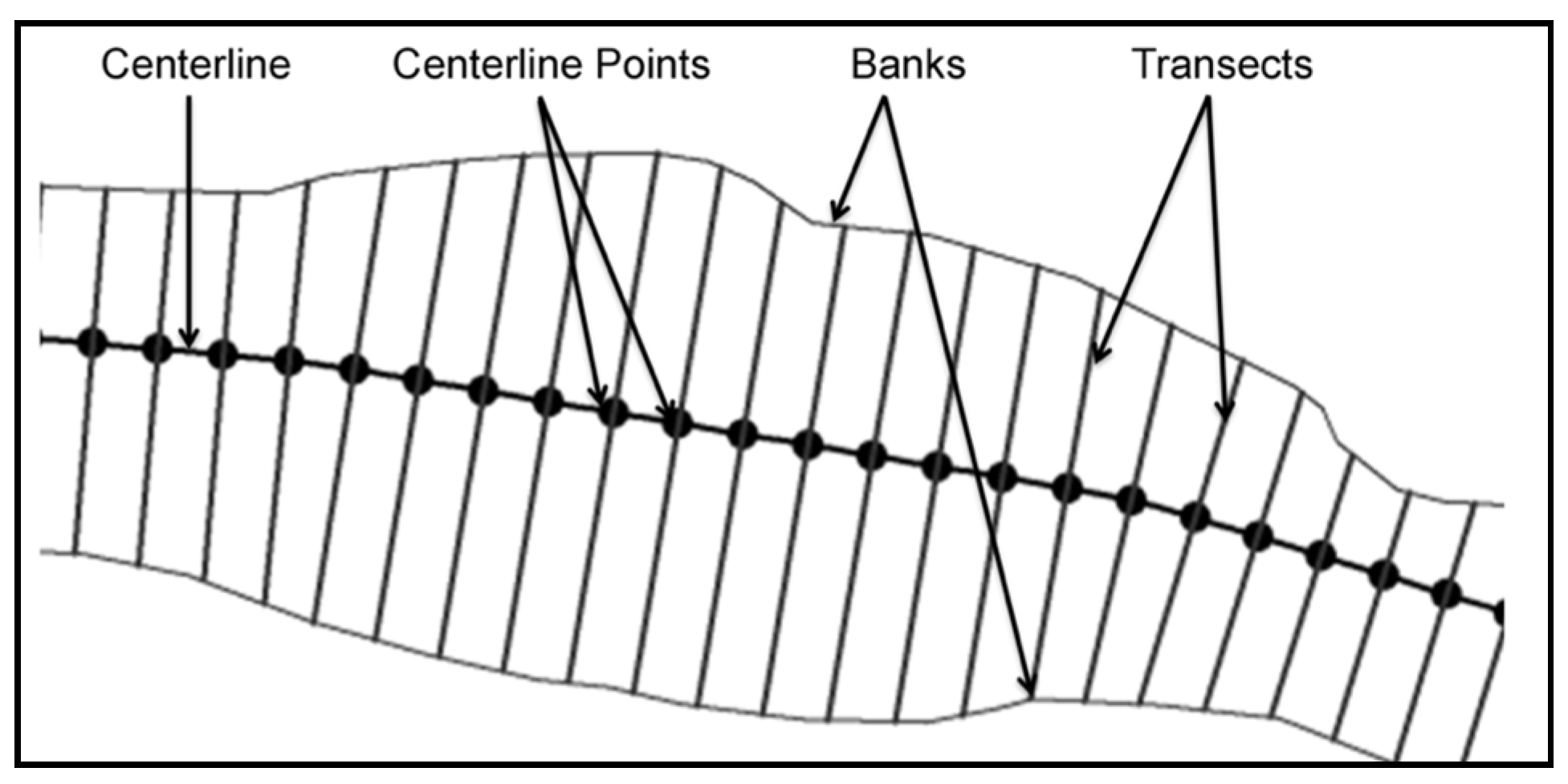
2.2. Geospatial Factors

2.3. Macroinvertebrate Sampling
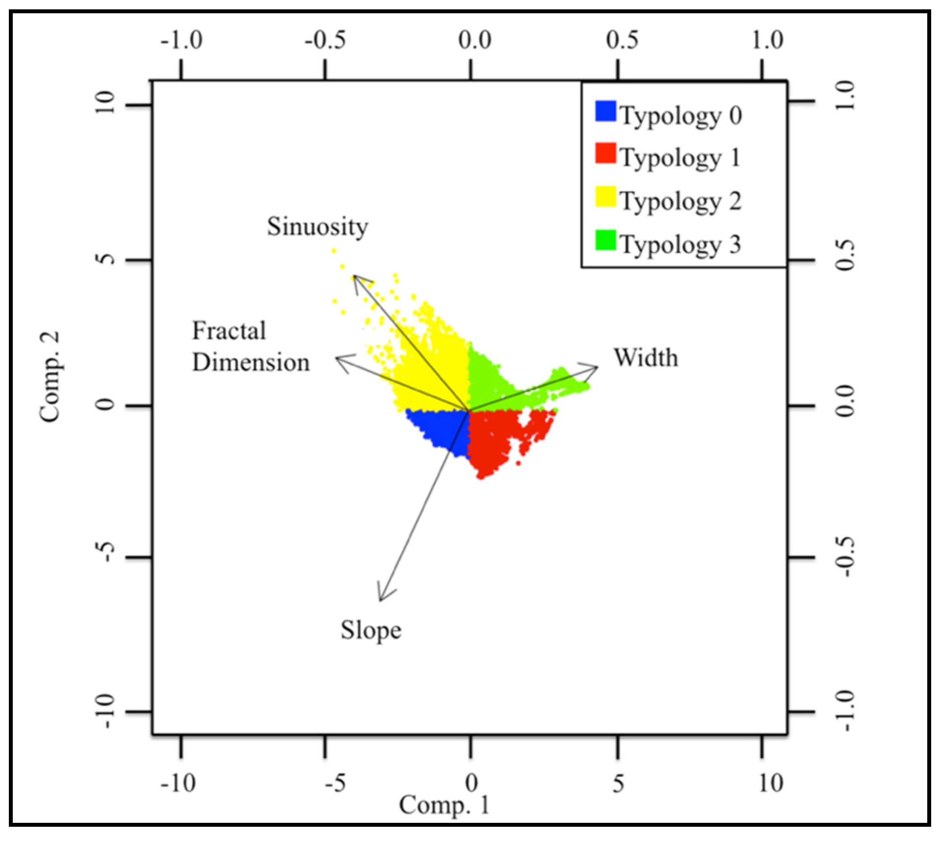
2.4. Statistical Analysis
3. Results and Discussion


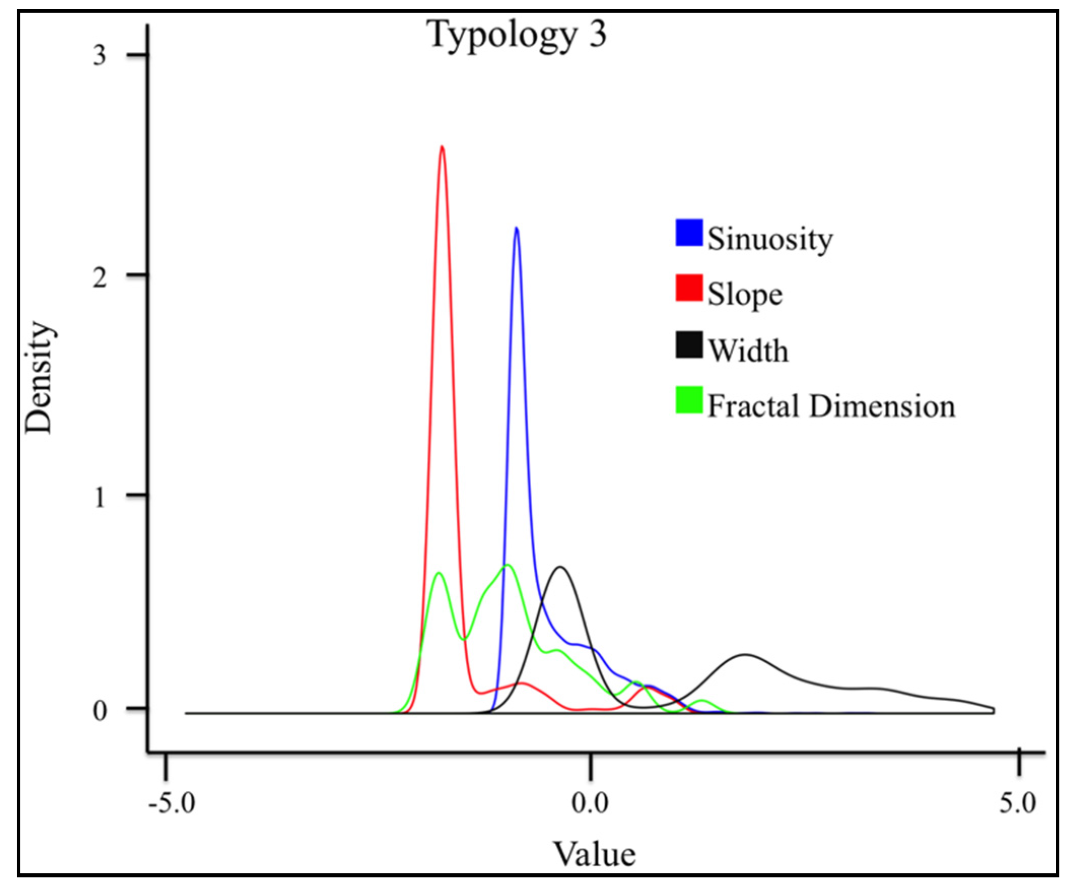
| Typology | Sinuosity | Slope | Fractal Dimension | Width |
|---|---|---|---|---|
| 0 | 0 | + | + | − |
| 1 | − | + | − | − |
| 2 | + | 0 | + | − |
| 3 | − | − | − | + |
3.1. Macroinvertebrate Survey
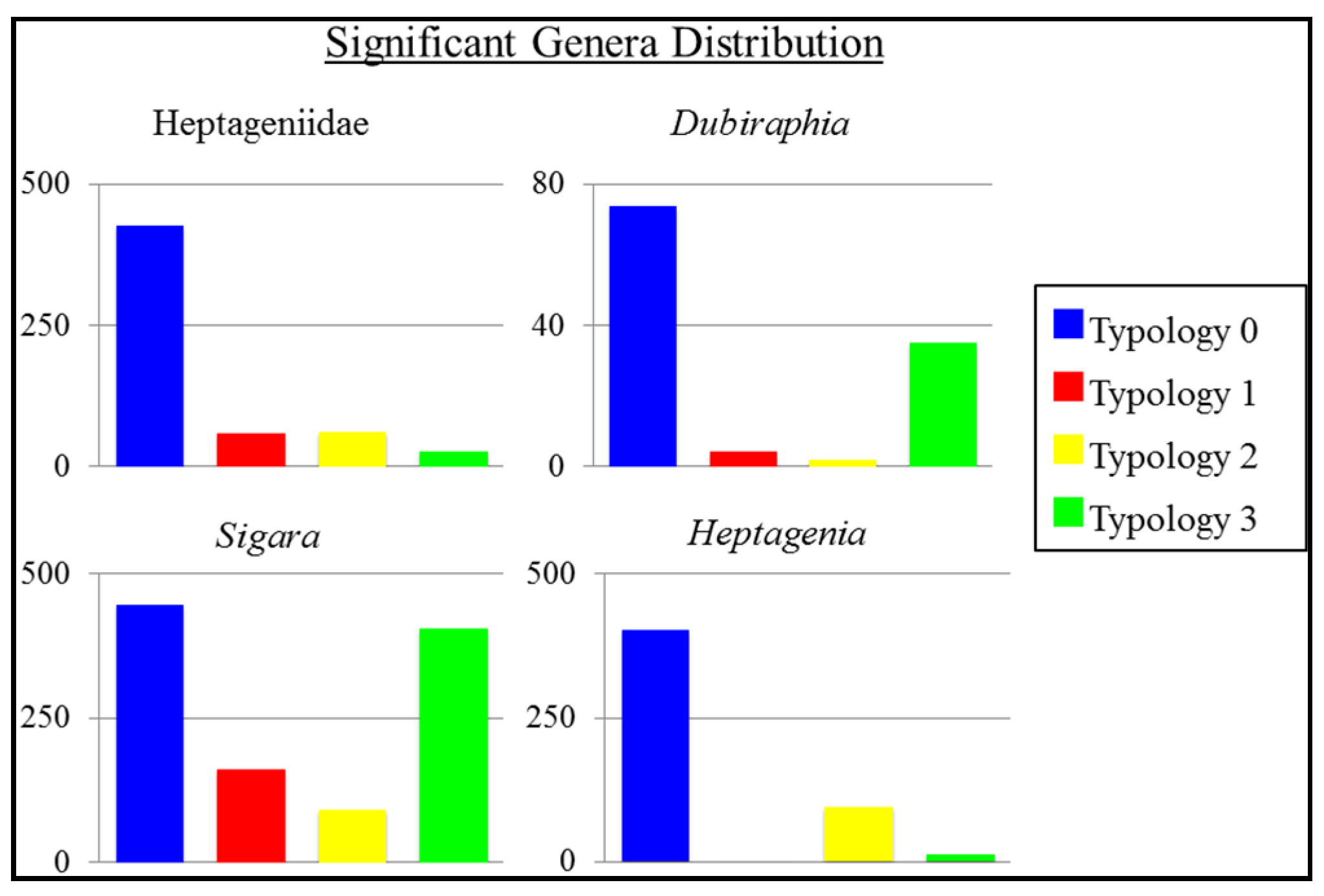
3.2. Statistical Analysis of Macroinvertebrate Survey
| Identifier | Order | Genus | H Value | df | p Value |
|---|---|---|---|---|---|
| G1 | Amphipoda | Amphipoda | 0.25 | 3 | 0.97 |
| G2 | Ephemeroptera | Baetidae | 4.2709 | 3 | 0.23 |
| G3 | Ephemeroptera | Baetis | 3.8312 | 3 | 0.28 |
| G4 | Trichoptera | Brachycentrus | 4.7699 | 3 | 0.19 |
| G5 | Ephemeroptera | Brachycercus | 1.03 | 3 | 0.79 |
| G6 | Ephemeroptera | Caenis | 2.2468 | 3 | 0.52 |
| G7 | Hemiptera | Callicorixa | 8.4314 | 3 | 0.04 * |
| G8 | Diptera | Ceratopogonidae | 0.0599 | 3 | 1 |
| G9 | Trichoptera | Cheumatopsyche | 2.1279 | 3 | 0.55 |
| G10 | Diptera | Chironomidae | 3.1975 | 3 | 0.36 |
| G11 | Hemiptera | Coenocorixa | 1.9423 | 3 | 0.58 |
| G12 | Hemiptera | Corixidae | 3.5733 | 3 | 0.31 |
| G13 | Lepidoptera | Crambidae | 3.8277 | 3 | 0.28 |
| G14 | Coleoptera | Dubiraphia | 8.0284 | 3 | 0.05 * |
| G15 | Odonata | Enallagma/Coenagrion | 5.0571 | 3 | 0.17 |
| G16 | Ephemeroptera | Ephemeridae/Polymitarcyidae | 2.9232 | 3 | 0.4 |
| G17 | Ephemeroptera | Ephemeroptera | 3.6787 | 3 | 0.3 |
| G18 | Ephemeroptera | Ephoron | 1.7929 | 3 | 0.62 |
| G19 | Amphipoda | Gammarus | 0.915 | 3 | 0.82 |
| G20 | Gastropoda | Gyraulus | 2.907 | 3 | 0.41 |
| G21 | Coleoptera | Haliplus | 7.9122 | 3 | 0.05 * |
| G22 | Ephemeroptera | Heptagenia | 9.5818 | 3 | 0.02 * |
| G23 | Ephemeroptera | Heptageniidae | 8.0369 | 3 | 0.05 * |
| G24 | Ephemeroptera | Hexagenia | 2.6277 | 3 | 0.45 |
| G25 | Amphipoda | Hyalella | 3.4018 | 3 | 0.33 |
| G26 | Hydrachnidia | Hydrachnidia | 1.4668 | 3 | 0.69 |
| G27 | Trichoptera | Hydropsyche | 1.7677 | 3 | 0.62 |
| G28 | Trichoptera | Hydropsychidae | 2.0198 | 3 | 0.57 |
| G29 | Trichoptera | Hydroptila | 3.5846 | 3 | 0.31 |
| G30 | Trichoptera | Hydroptilidae | 2.8369 | 3 | 0.42 |
| G31 | Trichoptera | Leptoceridae | 0.2782 | 3 | 0.96 |
| G32 | Gastropoda | Lymnaeidae | 4.4723 | 3 | 0.21 |
| G33 | Diptera/Trichoptera | Nectopsyche | 2.9025 | 3 | 0.41 |
| G34 | Oligochaeta | Oligochaeta | 2.5914 | 3 | 0.46 |
| G35 | Decopoda/Malacostraca | Orconectes | 4.4706 | 3 | 0.21 |
| G36 | Gastropoda | Physa | 7.1221 | 3 | 0.07 |
| G37 | Gastropoda | Physidae | 0.9604 | 3 | 0.81 |
| G38 | Pelecypoda | Pisidium | 2.0397 | 3 | 0.56 |
| G39 | Gastropoda | Planorbidae | 3.8277 | 3 | 0.28 |
| G40 | Gastropoda | Probythinella | 7.5965 | 3 | 0.06 |
| G41 | Hemiptera | Sigara | 8.0465 | 3 | 0.05 * |
| G42 | Diptera | Simulium | 6.5807 | 3 | 0.09 |
| G43 | Pelecypoda | Sphaeriidae | 3.1967 | 3 | 0.36 |
| G44 | Pelecypoda | Sphaerium | 6.9774 | 3 | 0.07 |
| G45 | Gastropoda | Stagnicola | 3.7902 | 3 | 0.29 |
| G46 | Ephemeroptera | Stenacron | 2.6016 | 3 | 0.46 |
| G47 | Ephemeroptera | Stenonema | 2.2751 | 3 | 0.52 |
| G48 | Hemiptera | Trichocorixa | 0.9051 | 3 | 0.82 |
| G49 | Ephemeroptera | Tricorythodes | 2.5764 | 3 | 0.46 |
| G50 | Gastropoda | Valvata | 7.3756 | 3 | 0.06 |
| Genus | 3 vs. 1 | 0 vs. 3 | 2 vs. 0 | ||||||
| ZV | PV | APV | ZV | PV | APV | ZV | PV | APV | |
| G7 | 2.246216 | 0.0124 | 0.0741 | −1.677963 | 0.0467 | 0.2801 | 1.785511 | 0.0371 | 0.2225 |
| G14 | −1.430855 | 0.0762 | 0.4574 | 0.868452 | 0.1926 | 1.0000 | 1.662240 | 0.0482 | 0.2894 |
| G21 | −0.469371 | 0.3194 | 1.0000 | 1.963520 | 0.0248 | 0.1488 | 0.253711 | 0.3999 | 1.0000 |
| G22 | −2.831301 | 0.0023 | 0.0139 * | 2.202077 | 0.0138 | 0.0830 | −1.148641 | 0.1254 | 0.7521 |
| G23 | −2.634423 | 0.0042 | 0.0253 * | 0.671864 | 0.2508 | 1.0000 | −0.407633 | 0.3418 | 1.0000 |
| G41 | −0.778480 | 0.2181 | 1.0000 | 1.138817 | 0.1274 | 0.7643 | 1.390046 | 0.0823 | 0.4935 |
| Genus | 0 vs. 1 | 2 vs. 1 | 2 vs. 3 | ||||||
| ZV | PV | APV | ZV | PV | APV | ZV | PV | APV | |
| G7 | 0.000000 | 0.5000 | 1.0000 | 2.167528 | 0.0151 | 0.0906 | 0.415734 | 0.3388 | 1.0000 |
| G14 | −0.207490 | 0.4178 | 1.0000 | 1.810392 | 0.0351 | 0.2107 | 2.817601 | 0.0024 | 0.0145 * |
| G21 | 1.669768 | 0.0475 | 0.2849 | 1.977762 | 0.0240 | 0.1439 | 2.261024 | 0.0119 | 0.0713 |
| G22 | 0.090114 | 0.4641 | 1.0000 | −1.304284 | 0.0961 | 0.5764 | 0.855175 | 0.1962 | 1.0000 |
| G23 | −1.341801 | 0.0898 | 0.5390 | −1.836650 | 0.0331 | 0.1988 | 0.193871 | 0.4231 | 1.0000 |
| G41 | 0.576929 | 0.2820 | 1.0000 | 2.264381 | 0.0118 | 0.0707 | 2.768790 | 0.0028 | 0.0169 * |

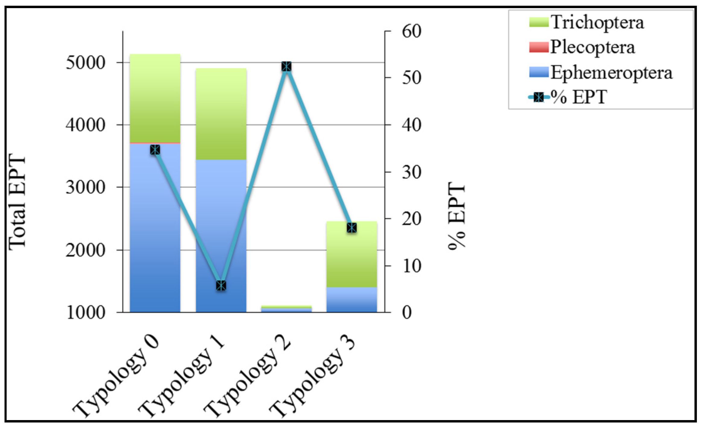
3.3. Ephemeroptera, Plecoptera, Trichoptera (EPT)
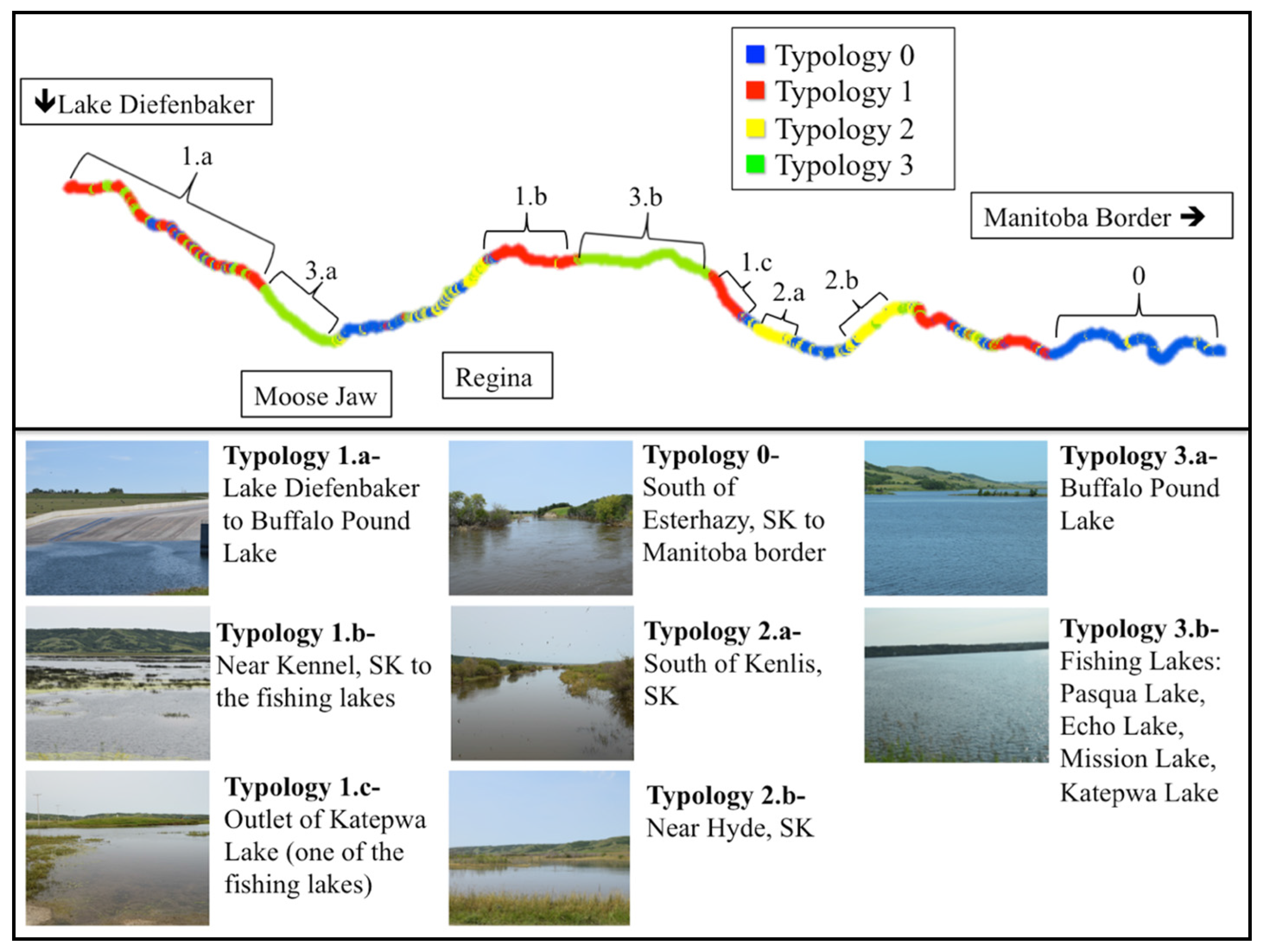
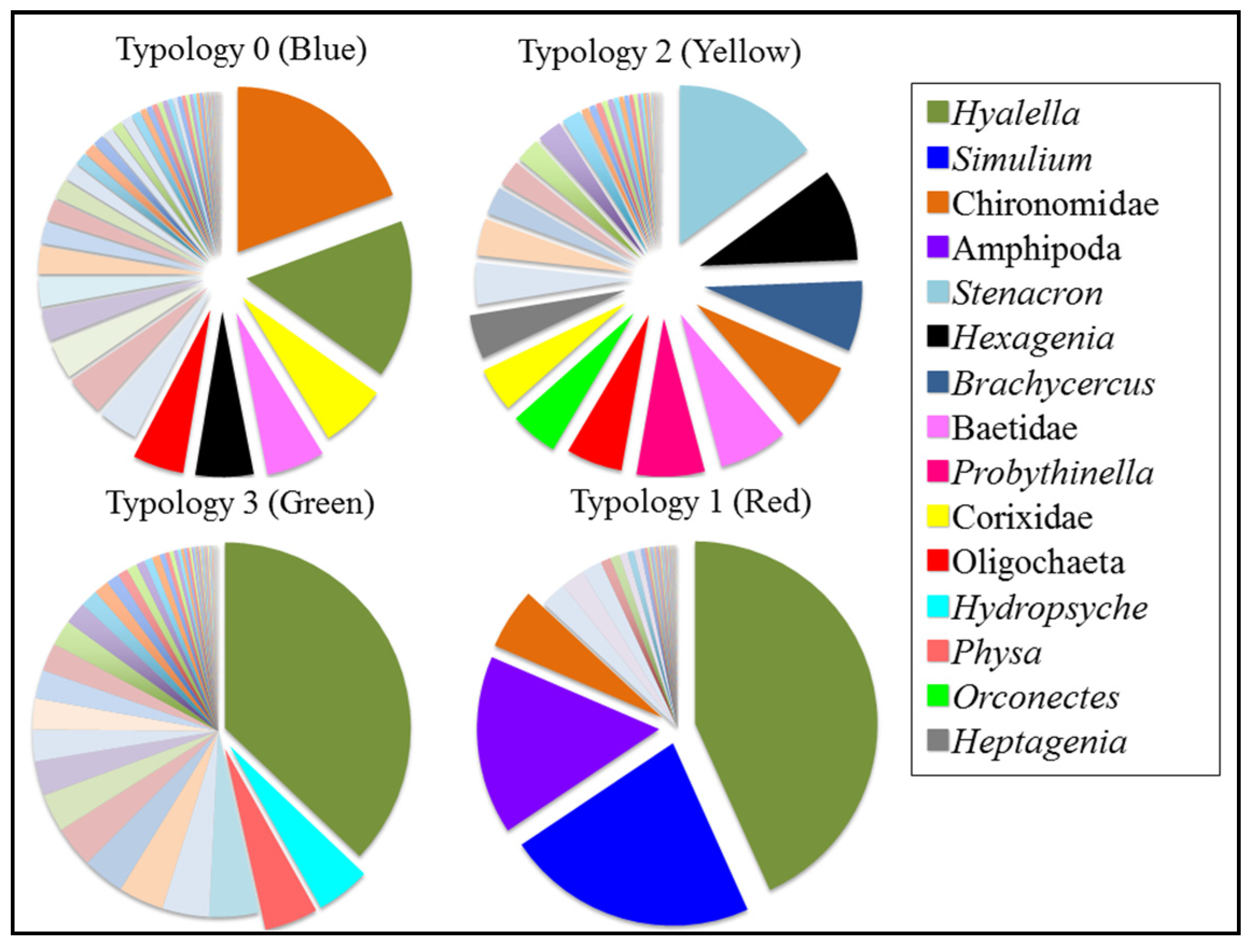
3.4. Geomorphological Typologies
3.4.1. Typology 0 (Blue)

3.4.2. Typology 1 (Red)
3.4.3. Typology 2 (Yellow)
3.4.4. Typology 3 (Green)
4. Conclusions
Acknowledgments
Author Contributions
Conflicts of Interest
References
- Larsen, J.; Birksl, H.J.B.; Raddum, G.G.; Fjellheim, A. Quantitative Relationships of Invertebrates to pH in Norwegian River Systems. Hydrobiologia 1996, 328, 57–74. [Google Scholar] [CrossRef]
- Whiles, M.R.; Brock, B.L.; Franzen, A.C.; Dinsmore, S.C. Stream Invertebrate Communities, Water Quality, and Land-Use Patterns in an Agricultural Drainage Basin of Northeastern Nebraska, USA. Environ. Manag. 2000, 26, 563–576. [Google Scholar] [CrossRef] [PubMed]
- Graf, W.; Murphy, J.; Zamora-Muñoz, C.; López-Rodríguez, M. Distribution and Ecological Preferences of European Freshwater Organisms; Pensoft Publishers: Sofia, Bulgaria, 2008. [Google Scholar]
- Altermatt, F.; Seymour, M.; Martinez, N. River Network Properties Shape α-Diversity and Community Similarity Patterns of Aquatic Insect Communities across Major Drainage Basins. J. Biogeogr. 2013, 40, 2249–2260. [Google Scholar] [CrossRef]
- Barton, D.R.; Farmer, M.E.D. The Effects of Conservation Tillage Practices on Benthic Invertebrate Communities in Headwater Streams in Southwestern Ontario, Canada. Environ. Pollut. 1997, 96, 207–215. [Google Scholar] [CrossRef]
- Morrissey, C.A.; Boldt, A.; Mapstone, A.; Newton, J.; Ormerod, S.J. Stable Isotopes as Indicators of Wastewater Effects On the Macroinvertebrates of Urban Rivers. Hydrobiologia 2013, 700, 231–244. [Google Scholar] [CrossRef]
- Dufrêne, M.; Legendre, P. Species Assemblages and Indicator Species: The Need for a Flexible Asymmetrical Approach. Ecol. Monogr. 1997, 67, 345–366. [Google Scholar] [CrossRef]
- Bonada, N.; Rieradevall, M.; Prat, N.; Resh, V.H. Benthic Macroinvertebrate Assemblages and Macrohabitat Connectivity in Mediterranean-Climate Streams of Northern California. J. N. Am. Benthol. Soc. 2006, 25, 32–43. [Google Scholar] [CrossRef]
- Kubosova, K.; Brabec, K.; Jarkovsky, J.; Syrovatka, V. Selection of Indicative Taxa for River Habitats: A Case Study on Benthic Macroinvertebrates Using Indicator Species Analysis and the Random Forest Methods. Hydrobiologia 2010, 651, 101–114. [Google Scholar] [CrossRef]
- Bovee, K.D.; Lamb, B.L.; Bartholow, J.M.; Stalnaker, C.B.; Taylor, J.; Henriksen, J. Stream Habitat Analysis Using the Instream Flow Incremental Methodology; U.S. Geological Survey, Biological Resources Division Information and Technology Report: Fort Collins, CO, USA, 1998. [Google Scholar]
- Gore, J.A.; Layzer, J.B.; Mead, J. Macroinvertebrate Instream Flow Studies after 20 Years: A Role in Stream Management and Restoration. Regul. River 2001, 17, 527–542. [Google Scholar] [CrossRef]
- Parasiewicz, P.; Dunbar, M.J. Physical Habitat Modelling for Fish—A Developing Approach. Large River 2001, 12, 239–268. [Google Scholar]
- Sanz-Ronda, F.J.; López-Sáenz, S.; San-Martín, R.; Palau-Ibars, A. Physical Habitat of Zebra Mussel (Dreissena Polymorpha) in the Lower Ebro River (Northeastern Spain): Influence of Hydraulic Parameters in Their Distribution. Hydrobiologia 2014, 735, 137–147. [Google Scholar] [CrossRef]
- Breiman, L. Random Forests. Mach. Learn. 2001, 45, 5–32. [Google Scholar] [CrossRef]
- Calow, P. A Method for Determining the Surface Areas of Stones to Enable Quantitative Estimates of Littoral Stone Dwelling Organisms to Be Made. Hydrobiologia 1972, 40, 37–50. [Google Scholar] [CrossRef]
- Cooper, C.M.; Testa, S., III. A Quick Method of Determining Rock Surface Area for Quantification of the Invertebrate Community. Hydrobiologia 2001, 452, 203–208. [Google Scholar] [CrossRef]
- Merritt, R.W.; Cummins, K.W.; Hunt, K. An Introduction to the Aquatic Insects of North America; Kendall/Hunt Publishing Company: Dubuque, IA, USA, 1996. [Google Scholar]
- Ernst, A.G.; Warren, D.R.; Baldigo, B.P. Natural-Channel-Design Restorations that Changed Geomorphology Have Little Effect on Macroinvertebrate Communities in Headwater Streams. Restor. Ecol. 2012, 20, 532–540. [Google Scholar] [CrossRef]
- Allan, J.D.; Castillo, M.M. Stream Ecology; Springer Science & Business Media: Dordrecht, The Netherlands, 2007. [Google Scholar]
- Dollar, E.S.J.; James, C.S.; Rogers, K.H.; Thoms, M.C. A Framework for Interdisciplinary Understanding of Rivers as Ecosystems. Geomorphology 2007, 89, 147–162. [Google Scholar] [CrossRef]
- Dodds, W.K.; Whiles, M.R. Freshwater Ecology: Concepts and Environmental Applications of Limnology; Academic Press: San Diego, CA, USA, 2010. [Google Scholar]
- Vannote, R.R.; Minshall, G.W.; Cummins, K.W.; Sedell, J.R.; Cushing, C.E. The River Continuum Concept. Can. J. Fish. Aquat. Sci. 1980, 37, 130–137. [Google Scholar] [CrossRef]
- Walters, D.M.; Leigh, D.S.; Freeman, M.C.; Pringle, C.M. Geomorphology and Fish Assemblages in a Piedmont River Basin, U.S.A. Freshw. Biol. 2003, 48, 1950–1970. [Google Scholar] [CrossRef]
- Holyoak, M.; Leibold, M.A.; Holt, R.D. Metacommunities: Spatial Dynamics and Ecological Communities; University of Chicago Press: Chicago, IL, USA, 2005. [Google Scholar]
- Rodríguez-Iturbe, I.; Valdés, J.B. The Geomorphologic Structure of Hydrologic Response. Water. Resour. Res. 1979, 15, 1409–1420. [Google Scholar] [CrossRef]
- Carrara, F.; Altermatt, F.; Rodríguez-Iturbe, I.; Rinaldo, A. Dendritic Connectivity Controls Biodiversity Patterns in Experimental Metacommunities. Proc. Natl. Acad. Sci. USA 2012, 109, 5761–5766. [Google Scholar] [CrossRef] [PubMed]
- D’Ambrosio, J.L.; Williams, L.R.; Witter, J.D.; Ward, A.D. Effects of Geomorphology, Habitat, and Spatial Location on Fish Assemblages in a Watershed in Ohio, USA. Environ. Monit. Assess. 2009, 148, 325–341. [Google Scholar] [CrossRef] [PubMed]
- Lindenschmidt, K.-E.; Long, J. A GIS Approach to Define the Hydro-Geomorphological Regime for Instream Flow Requirements Using Geomorphic Response Units (GRU). River Syst. 2013, 20, 261–275. [Google Scholar] [CrossRef]
- Milner, V.S.; Gilvear, D.J. Characterization of Hydraulic Habitat and Retention across Different Channel Types: Introducing a New Field-Based Technique. Hydrobiologia 2012, 694, 219–233. [Google Scholar] [CrossRef]
- Charlton, R. Fundamentals of Fluvial Geomorphology; Routledge: Abingdon, UK, 2008. [Google Scholar]
- Mollard, J.D. Morphological Study of the Upper Qu’Appelle River; Friends of Wascana Marsh: Regina, SK, Canada, 2004. [Google Scholar]
- Nature Conservancy Canada. Qu’Appelle River Valley. Available online: http://www.natureconservancy.ca/en/where-we-work/saskatchewan/our-work/qu-appelle_river_valley.html (accessed on 10 October 2015).
- Clifton Associates Ltd. Upper Qu’Appelle Water Supply Project: Economic Impact and Sensitivity Analysis; Water Security Agency: Regina, SK, Canada, 2012. [Google Scholar]
- Saskatchewan Watershed Authority. Getting to the Source Upper Qu’Appelle River and Wascana Creek Watersheds Source Water Protection Plan; Upper Qu’Appelle River and Wascana Creek Watersheds Advisory Committees: Regina, SK, Canada, 2008. [Google Scholar]
- Pittman, J.; Pearce, T.; Ford, J. Adaptation to Climate Change and Potash Mining in Saskatchewan: Case Study from the Qu’Appelle River Watershed; Climate Change Impacts and Adaptation Division, Natural Resources Canada: Ottawa, ON, Canada, 2013. [Google Scholar]
- MathSoft Inc. Mathcad v.15; MathSoft Inc.: Cambridge, MA, USA, 2012. [Google Scholar]
- Güneralp, İ.; Abad, J.D.; Zolezzi, G.; Hooke, J. Advances and Challenges in Meandering Channels Research. Geomorphology 2012, 163–164, 1–9. [Google Scholar] [CrossRef]
- Ahnert, F. Einführung in Die Geomorphologie; Verlag Eugen Ulmer: Stuttgart, Germany, 2015. [Google Scholar]
- Lüderitz, V.; Kunz, C.; Wüstemann, O.; Remy, D.; Feuerstein, B. Typisierung und Bewertung für die leitbildorientierte Sanierung von Altwässern. In Flussaltwässer: Ökologie und Sanierung; Lüderitz, V., Langheinrich, U., Kunz, C., Eds.; Vieweg + Teubner: Wiesbaden, Germany, 2009; pp. 91–168. [Google Scholar]
- Zumbroich, T.; Müller, A. Das Verfahren der Gewässerstrukturkartierung. In Strukturgüte von Fließgewässern: Grundlagen und Kartierung, 1st ed.; Zumbroich, T., Müller, A., Günther, F., Eds.; Springer-Verlag: Heidelberg, Germany; Berlin, Germany, 1999; pp. 97–121. [Google Scholar]
- Schumm, S.A. The Fluvial System; John Wiley & Sons: New York, NY, USA, 1977; p. 338. [Google Scholar]
- Shen, X.H.; Zou, L.J.; Zhang, G.F.; Su, N.; Wu, W.Y.; Yang, S.F. Fractal Characteristics of the Main Channel of Yellow River and Its Relation to Regional Tectonic Evolution. Geomorphology 2011, 127, 64–70. [Google Scholar] [CrossRef]
- Knighton, D. Fluvial Forms and Processes: A New Perspective; Routledge: New York, NY, USA, 1998. [Google Scholar]
- Schuller, D.J.; Rao, A.R.; Jeong, G.D. Fractal Characteristics of Dense Stream Networks. J. Hydrol. 2001, 243, 1–16. [Google Scholar] [CrossRef]
- R Development Core Team. R: A language and Environment for Statistical Computing; R Foundation for Statistical Computing: Vienna, Austria, 2012; Available online: https://www.r-project.org/ (accessed on 10 September 2015).
- Legendre, P.; Legendre, L. Numerical Ecology, 3rd ed.; Elsevier: Amsterdam, The Netherlands, 2012. [Google Scholar]
- Dosdall, L.M.; Lehmkuhl, D.M. Stoneflies (Plecoptera) of Saskatchewan. Quaest. Entomol. 1979, 15, 3–116. [Google Scholar]
- Clifford, H.F. Aquatic Invertebrates of Alberta; The University of Alberta Press: Edmonton, AB, Canada, 1991. [Google Scholar]
- Webb, J.M. The Mayflies of Saskatchewan. Master’s Thesis, University of Saskatchewan, Saskatoon, SK, Canada, 2002. [Google Scholar]
- O’Laughlin, K. The Streamkeeper’s Field Guide: Watershed Inventory and Stream Monitoring Methods; Adopt-A-Stream Foundation: Washington, DC, USA, 1996. [Google Scholar]
- Karaus, U.; Larsen, S.; Guillong, H.; Tockner, K. The Contribution of Lateral Aquatic Habitats to Insect Diversity along River Corridors in the Alps. Landsc. Ecol. 2013, 28, 1755–1767. [Google Scholar] [CrossRef]
- Mandaville, S.M. Benthic Macroinvertebrates in Taxa Tolerance Values, Metrics, and Protocols; Project H-1; Soil and Water Conservation Society of Metro Halifax: Halifax, NS, Canada, 2002. [Google Scholar]
- Eymann, M. Flow Patterns Around Cocoons and Pupae of Black Flies of the Genus Simulium (Diptera: Simuliidae). Hydrobiologia 1991, 215, 223–229. [Google Scholar] [CrossRef]
- Eymann, M.; Friend, W.G. Behaviors of Larvae of the Black Flies Simulium Vittatum and S. Decorum (Diptera: Simuliidae) Associated with Establishing and Maintaining Dispersion Patterns on Natural and Artificial Substrates. J. Insect Behav. 1988, 1, 169–186. [Google Scholar] [CrossRef]
- Government of Canada Fisheries and Oceans. Manual for the Culture of Selected Freshwater Invertebrates; Lawrence, S.G, Ed.; Department of Fisheries and Oceans Freshwater Institute: Winnipeg, MB, Canada, 1981. [Google Scholar]
- Doll, B.A.; Jennings, G.G.; Spooner, J.; Penrose, D.L.; Usset, J.L. Evaluating the Eco–Geomorphological Condition of Restored Streams Using Visual Assessment and Macroinvertebrate Metrics. J. Am. Water Resour. Assoc. 2015, 51, 68–83. [Google Scholar] [CrossRef]
- D’Ambrosio, J.L.; Williams, L.R.; Williams, M.G.; Witter, J.D.; Ward, A.D. Geomorphology, Habitat, and Spatial Location Influences on Fish and Macroinvertebrate Communities in Modified Channels of an Agriculturally-Dominated Watershed in Ohio, USA. Ecol. Eng. 2014, 68, 32–36. [Google Scholar] [CrossRef]
© 2016 by the authors; licensee MDPI, Basel, Switzerland. This article is an open access article distributed under the terms and conditions of the Creative Commons by Attribution (CC-BY) license (http://creativecommons.org/licenses/by/4.0/).
Share and Cite
Meissner, A.G.N.; Carr, M.K.; Phillips, I.D.; Lindenschmidt, K.-E. Using a Geospatial Model to Relate Fluvial Geomorphology to Macroinvertebrate Habitat in a Prairie River—Part 1: Genus-Level Relationships with Geomorphic Typologies. Water 2016, 8, 42. https://doi.org/10.3390/w8020042
Meissner AGN, Carr MK, Phillips ID, Lindenschmidt K-E. Using a Geospatial Model to Relate Fluvial Geomorphology to Macroinvertebrate Habitat in a Prairie River—Part 1: Genus-Level Relationships with Geomorphic Typologies. Water. 2016; 8(2):42. https://doi.org/10.3390/w8020042
Chicago/Turabian StyleMeissner, Anna G. N., Meghan K. Carr, Iain D. Phillips, and Karl-Erich Lindenschmidt. 2016. "Using a Geospatial Model to Relate Fluvial Geomorphology to Macroinvertebrate Habitat in a Prairie River—Part 1: Genus-Level Relationships with Geomorphic Typologies" Water 8, no. 2: 42. https://doi.org/10.3390/w8020042