1. Introduction
Separate sewer discharges are now widely recognized for their deleterious impact on receiving water bodies. Although combined sewer overflows were traditionally considered to be the major cause of water quality degradation in urban waterways, the impacts of stormwater discharges has been recently attracting more attention with separate networks taking over combined ones [
1,
2,
3]. The high levels of pollution frequently observed in stormwater outflows are shown to significantly contribute to the environmental pressure of urban areas on water streams, from which the importance of a proper evaluation of these discharges emerges [
4,
5].
The modelling of urban stormwater can be split into two components: the simulation of water quantity and the simulation of water quality. Despite the rapid development of hydrological modelling during last decades, the water quality component of urban stormwater modelling remains far less studied. One of the main reasons is that accurate simulations of pollutant transport on urban surfaces require detailed spatial and temporal information on stormwater runoff [
6,
7]. For example, surface modules of the well-known SWMM [
8] and MUSIC [
9] models are respectively based on examining sub-catchments and land-use parcels to simulate overland flows in urban catchments. These approaches are based on a conceptual representation of routing processes governing pollutants’ transport from their generation points to the sub catchment outlet [
10]. Most of them are based on Sartor and Boyd formulations of build-up and wash-off on urban surfaces [
11]. These conceptual equations have been criticized by several authors [
7,
12,
13,
14] for their poor performance in reproducing pollutant concentration dynamics. However, current urban stormwater quality models (e.g., SWMM, MUSIC, etc.) still rely on these empirical catchment-scale functions that have not substantially evolved over the last 40 years. An alternative way to improve their performance might be to even out their spatial dimension applications. In this respect, the 2D erosion model (TREX), which was initially developed for rural/agricultural catchments and largely tested by the scientific community to simulate particle transport in natural catchments, represents an interesting tool to apply to urban catchments. This novel modelling approach could lend itself to new ways of thinking in the field of urban stormwater quality modelling, and could potentially advance our modelling techniques.
Over the last few years, the modeling approach of combining 2D overland flow and 1D drainage sewer flow has received great attention [
15,
16]. Several research models [
17,
18,
19,
20] and commercial tools [
21,
22] have already been developed and applied to various case studies. These models are able to accurately represent the spatial and temporal variations of surface runoffs and sewer flows on urban areas. The concept of these 2D/1D models is hence well adapted to introducing more reliable pollutant transport processes. However, present applications of these models are mostly focused on urban flood modelling, while being rarely investigated for urban pollutant transport simulations. On the other hand, existing publications on integrated 2D/1D models rarely compare the influences of different factors on model outputs [
16,
23,
24]. In that case, the main drivers of the model outputs are still not sufficiently investigated, which decreases the reliability of the integration of new processes into the existing model, and restricts the transferability of the model to other case studies.
In this context, we coupled the physically-based 2D model TREX [
25,
26], which has been initially developed for watershed rainfall-runoff, sediment and contaminant transport modelling, with the 1D pipe routing and subbasin components of the CANOE model [
27], resulting in the “TRENOE” platform. It is the first time that such a 2D physically-based erosion model, based on USLE equations, has been coupled with an urban model for the simulation of urban stormwater quality. Moreover, TREX is an open source code, well-documented, with a robust numerical scheme, which makes it suitable for modification in an urban context. The coupling between TREX and CANOE models is designed to be able to simulate the 2D overland flows and the 1D sewer network routing. Roofs are simulated separately from the 2D surface model in TRENOE. Since the roof gutters are connected directly to the sewer networks in the studied catchment, roofs are represented as the “subbasins” in the 1D CANOE model.
Within the framework of the ANR (French National Agency for Research) Trafipollu project, a detailed Geographic Information System (GIS) database is available for the study of urban catchments (Le Perreux sur Marne, 0.12 km2), such as by using the high-resolution topographic data of LiDAR survey and the detailed land use data derived from ortho photos. Benefitting from this large dataset of detailed source data and continuous measurement at the sewage outlet, the influences of various inherent (model structure, numerical issues) and external (input-data, parameter values) factors on model performance are evaluated.
In general, this paper focus on two objectives: firstly, to apply the physically-based 2D/1D TRENOE platform to urban stormwater quantity and quality modelling; secondly, to rank the impacts of different factors on model outputs and to highlight the prerequisites for high performance simulations. The results of this study may be very useful for reducing the cost of urban stormwater management by avoiding some unnecessary data acquisition and modelling efforts (high-resolution topograhic data, calibration, etc.). Perspectives and propositions for improving urban stormwater quality modelling are presented as well.
2. Materials and Methods
2.1. Model Description
The physically-based 2D model TREX and the 1D pipe routing and subbasin components of the CANOE model are integrated into the TRENOE platform. Within TREX, the catchment surface is divided into several rectangular meshes based on GIS topographic data. These grids are then categorized into several classes according to land use information. Different parameters are attributed to each grid point in accordance with the land use type. Interception, infiltration, water runoff and pollutant transfer processes are then calculated. Diffusive wave approximation of Shallow-Water equations (SW) is applied for simulating the surface runoff at the grid scale, which is able to represent the spatial and temporal variations of the water flow and the associated pollutants. With the 1D sewer system CANOE model, stormwater and pollutant routing processes are computed for each portion of pipes between pre-defined junction nodes using the kinematic approximation of SW equations and advection equations, respectively. The modelling processes in TRENOE are described in
Table 1.
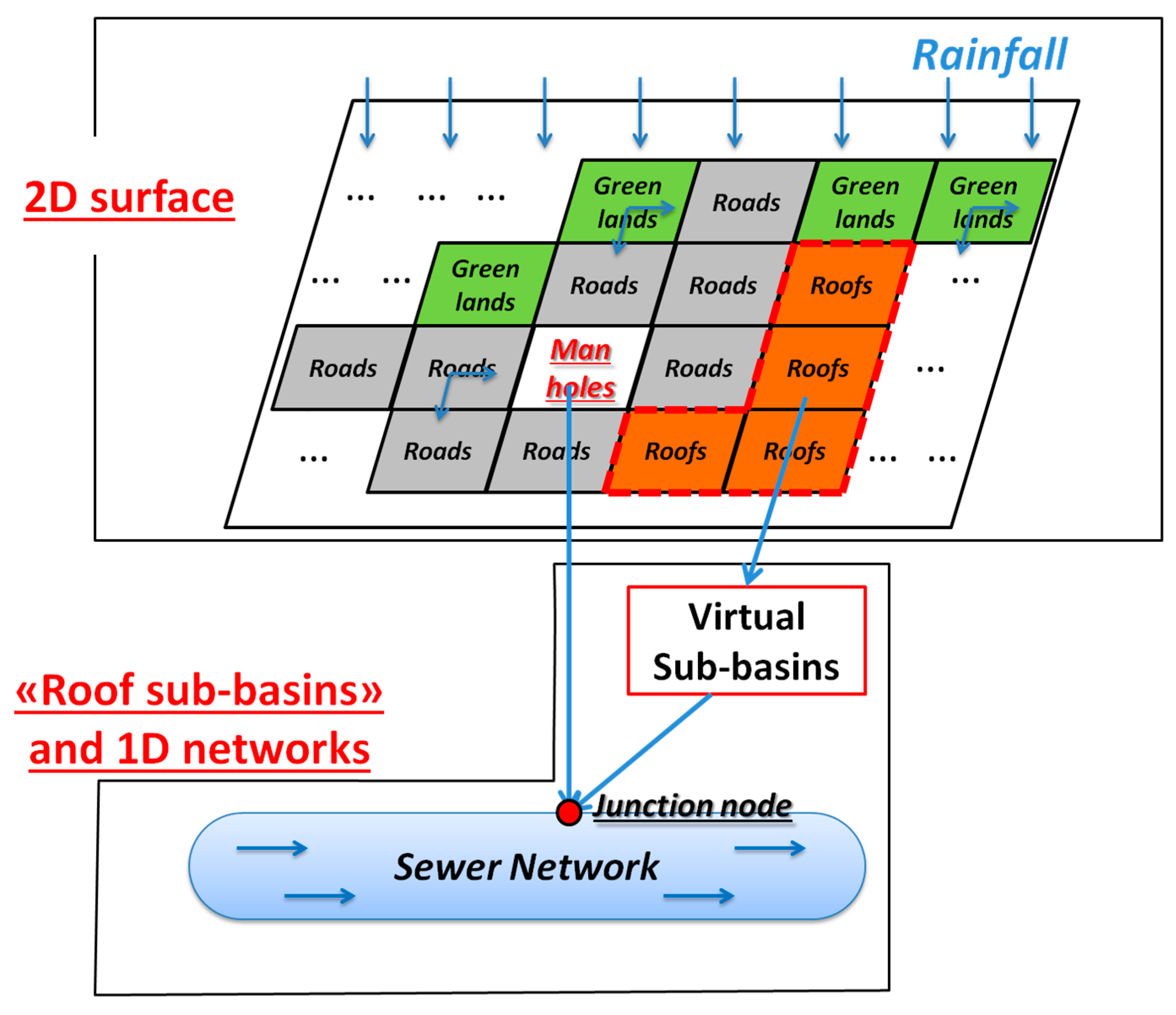
The “junction nodes” in 1D sewer network model are the connecting points between different parts of the TRENOE platform. From the grids of “sewer inlets” and “roofs”, water and pollutants flow directly into the sewer networks via these “junction nodes”. “Sewer inlets” are considered as “holes” in the 2D surface model, where surface runoff and the related pollutants disappear at these grid points. In contrast, “roofs” are represented as obstacles, where water flows cannot enter these grids from other types of land uses. As the buildings are not described in the Digital Elevation Model (DEM) data, the grids of “roofs” are increased by 5 m at the step of input data pre-treatment. Since most roofs are directly connected to the sewer networks in the studied urban catchment, we gather the grids of roofs which are linked to the same junction nodes (the nearest), to set the conceptual “sub-catchments” in CANOE model. The size of each “sub-catchment” is equal to the total area of the linking “roofs” grids. The non-linear reservoir method and the exponential washoff equations [
13] are then applied to simulate the rainfall-runoff and the pollutant transport, respectively, for each conceptual “sub-catchment”. The model scheme is illustrated in
Figure 1.
2.2. Study Site and Urban Catchment Delineation
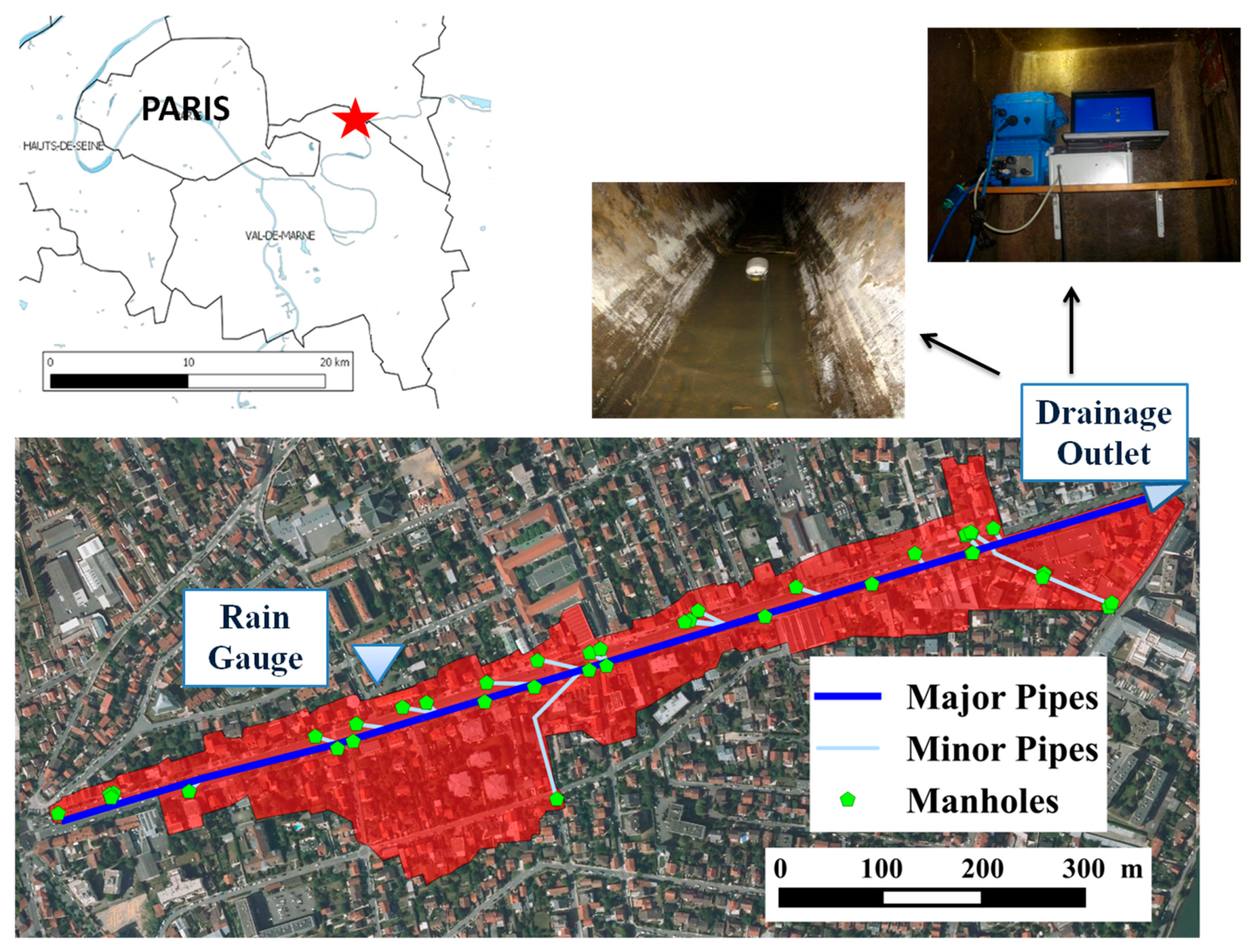
The study site is located in the eastern suburb of Paris (Le Perreux sur Marne, Val de Marne, France). This research area is a typical residential zone in the Paris region, characterized by a highly trafficked main street of eastern Paris. A preliminary step is to delineate the urban catchment. Since this study aims at precisely modelling water flows and pollutant transport at small urban scales, a detailed delineation of the urban catchment is necessary. As it is well-known that the urban areas are complex because of various buildings and infrastructure that may influence the water flow path, our “hand-operated” delineation procedure is based on the complete knowledge of sewer network infrastructure, road high-resolution LiDAR data (20 cm), and the Digital Orthophoto Quadrangles (DOQs) (5 cm).
The detailed urban catchment is delimited by applying the following steps: (i) identifying the contributing sewage portions for the monitored drainage outlet using elaborate sewer network data; (ii) locating the sewer inlets; (iii) delimiting the “drainage basin” for each sewer inlet benefiting from the road high-resolution LiDAR data (20 cm); (iv) merging all the “drainage basins” defined by the precedent steps; (v) comparing data with the DOQs (5 cm), recognizing the buildings and infrastructure that should be included in the basin. The delimited urban catchment is presented in
Figure 2.
2.3. Input Data Description
2.3.1. Rainfall Data
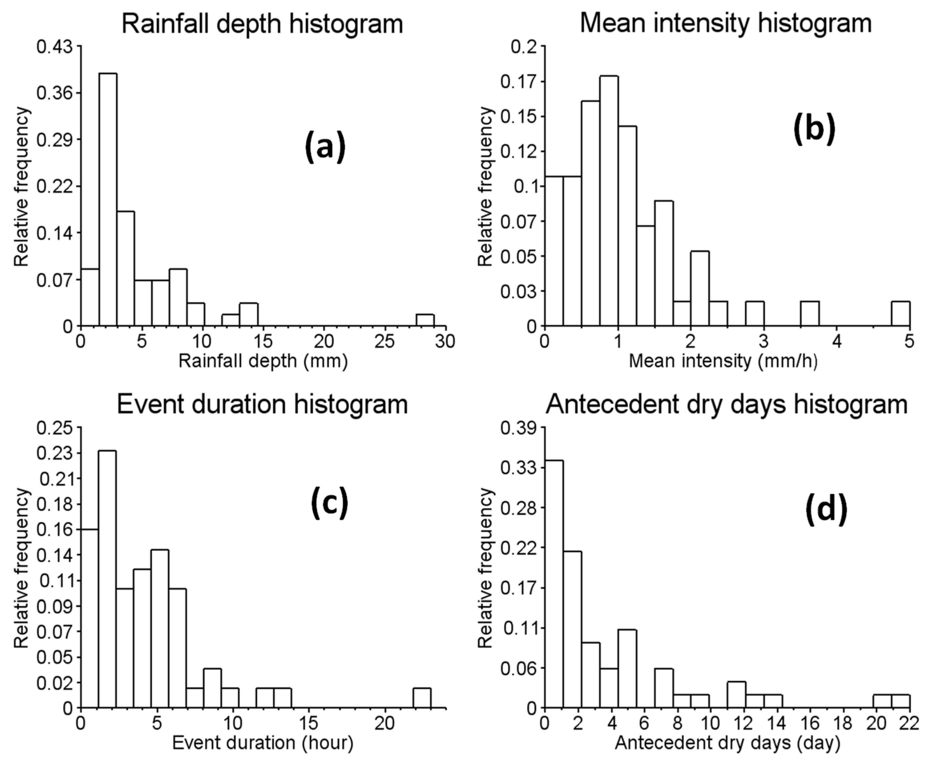
A tipping-bucket rain gauge is installed on the roof of a building close to the urban catchment (less than 150 m). The pluviometer has a resolution of 0.1 mm. As the study area is quite small, rainfall is considered as homogeneous within the basin. Monitoring was conducted between 20 September 2014 and 27 April 2015. Different rainfall events are identified by the time intervals longer than 90 min between two tipping records and the total rainfall depth of each event should be more than 1 mm. At the end, 56 rainfall events have been recognized for the observed period. An analysis of rainfall depth, mean intensity, event duration and antecedent dry days is performed for all rainfall events in order to analyze their characteristics (
Figure 3).
According to
Figure 3a,b, we can observe that most rainfall events within the study area of eastern Paris are considered low. In fact, more than 88% of rainfall events have a rainfall depth of less than 8 mm, and nearly 89% of rainfall events have a mean intensity lower than 3 mm/h. Additionally,
Figure 3c,d shows that event duration and antecedent dry days are a little more heterogeneous. However, most rainfall events observed are shorter than 7 h (87%), while 88% of the events are preceded by a previous rainfall event by less than 8 days. As the simulations are quite time-consuming, we have to select several rainfall events which contain different characteristics in order to characterize the overall performance of the TRENOE platform within an urban context. Among the rainfall events observed, we selected 6 typical events for model application and performance evaluation. A summary of selected rainfall events is listed in
Table 2.
2.3.2. Topographic Data
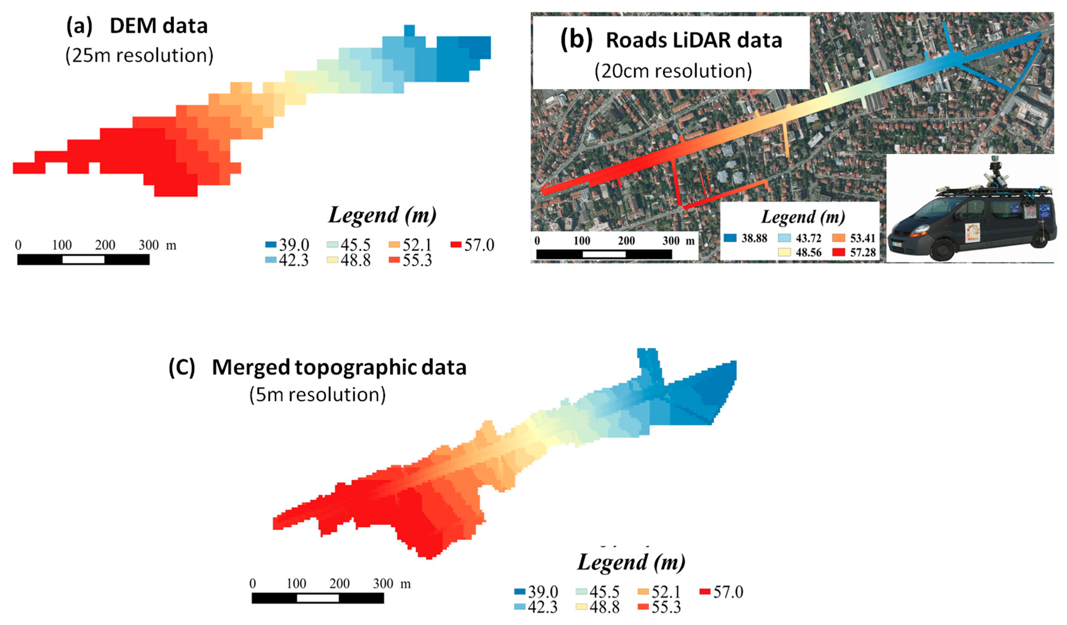
Topographic data is a crucial input for physically based modelling. In the GIS database of the Paris region, the 25 m-resolution DEM data is available (
Figure 4a). Moreover, in the framework of the ANR-Trafipollu project, the LiDAR data of roads collected by IGN France have a horizontal resolution of 20 cm and a vertical precision of 1 cm. These data were collected by an on-vehicle laser (
Figure 4b). The roads are essential flow pathways in the studied urban catchment, because the surrounding roofs are directly connected to the sewer network and the greenlands only represent a small part of the urban surface. Therefore, the topographic data of roads derived from high resolution LiDAR data improve the resolution and precision of previously used DEM data. Nevertheless, the resolution used for the TREX-CANOE simulation platform needs to aggregate the Lidar data and thus to lower their original resolution. Following [
29,
30], the proper spatial resolution for 2D modelling of the urban surface can be set by considering the minimum distance between buildings and one third of the street width as well as the calculation time. For our case study, this distance can be estimated to 5 m. Compared with the DEM data at a 25 m resolution, the use of high resolution LiDAR is a significant improvement, even for the simulations performed at 5 m resolution. Thereupon, both 20 cm and 25 m resolution topographic data are firstly converted to 5 m resolution, and then merged to generate the input data. The merged topographic data of 5 m resolution is presented in
Figure 4c, in which the study catchment is represented by a 224 × 85 rectangular grid.
2.3.3. Land Use and Sewer Network
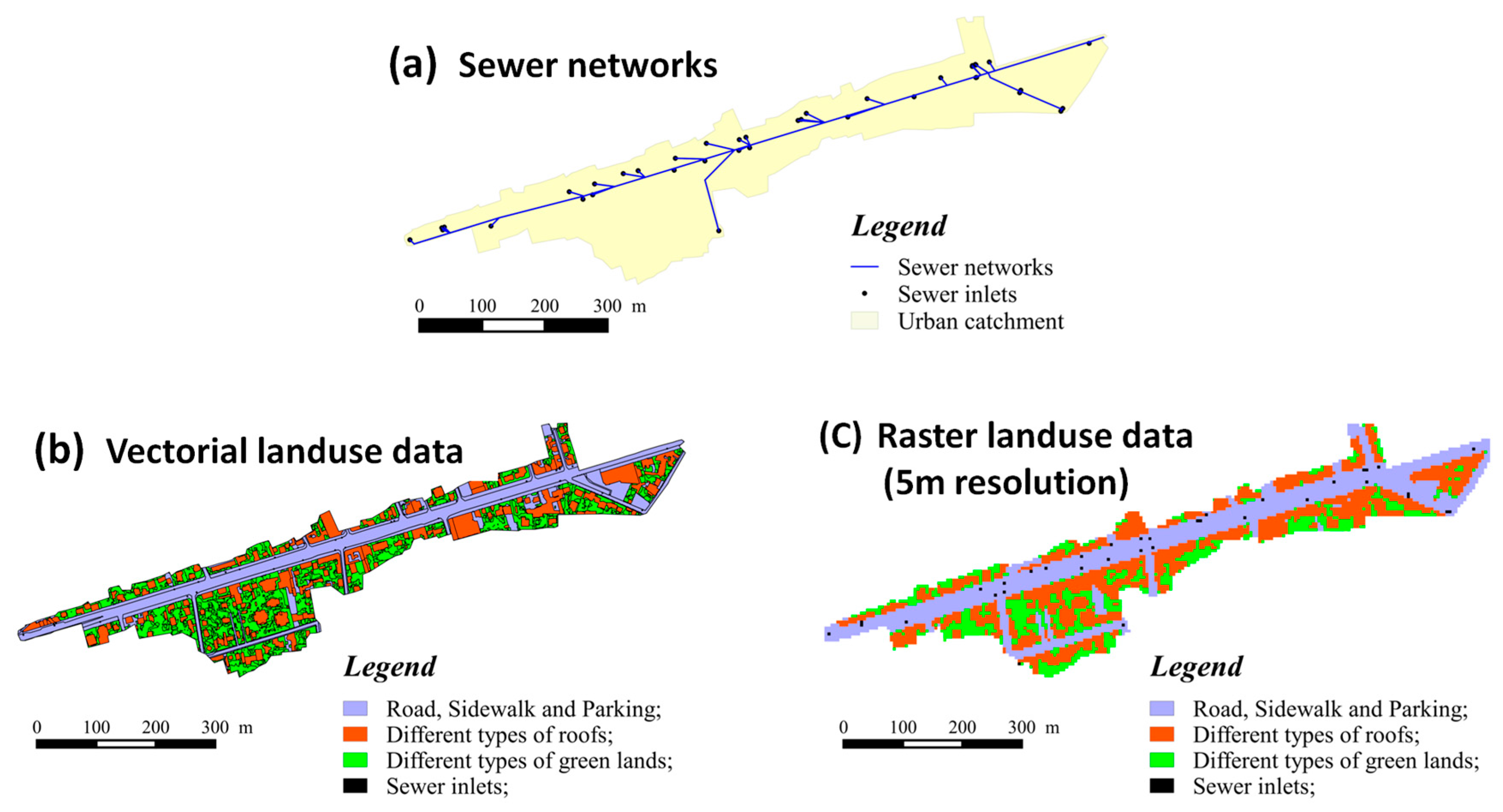
In collaboration with the IGN France, we defined 13 classes of urban land uses which are derived from aerial photos. Besides, the locations of sewer inlets are identified from the GIS and AutoCAD sewer network data. Since sewer inlets should equally be presented in the surface part of the 2D/1D model, the “sewer inlets” are integrated into land use input as a specific type. The vectorial land uses are then transformed into grids using the same resolution as the topographic data. A specific order has to be defined for this transformation. As the “sewer inlets” are considered as the interface between the surface and sewer networks parts, it is undoubted that the “Sewer inlet” is the first that should be considered, followed by roads, sidewalks, parking, various types of roofs, trees, grass and others. In general, 70% of catchment surfaces are impervious areas, within which the roof areas represent 35% of the total surface. The land use data and sewer network data are presented in
Figure 5.
2.3.4. Urban Surface Dry Stocks
Impervious urban surfaces are represented by two layers in TRENOE: the deposited layer (that can be detached in the form of particles) and the pavement (assumed to be non-detachable). The processes related to water quality modelling occur only in the deposited layer, while the parameters depend on the properties of the associated land use. Additionally, within the framework of the ANR-Trafipollu project, series of road dust samples were collected on the studied area using a 2 m
2 vacuum cleaner [
31]. The collected road dust Particle Size Distribution (PSD) was then determined by laboratory monitoring. According to the measurements of dry stock samples over 3 different sites on the urban surface, it is assumed that the finest particles (PM10) are only generated by atmospheric dry deposits on all types of urban surfaces. The total dry stock on roads (coarse + fine particles) was estimated to 10 g/m
2. The mass of the finest part of the road dry deposits which represent the atmospheric dry depositions is then estimated to be 1 g/m
2. Therefore, it is considered that building roof accumulation is equal to the finest deposits on roads, and the chosen initial dry deposits on roofs are 1 g/m
2 in our simulations.
2.4. Model Evaluation with Scenario Simulations
Due to time-consuming simulations with the physically-based TRENOE platform (using a computer core of 16 GB RAM, the model runtime is approximately 10 min for a 1-h rainfall event), the model assessment is performed by scenario simulations instead of complete sensitivity analysis. Model configurations are firstly calibrated by a trial and error method comparing with water flow measurements at the sewage outlet. The influences of various factors are then examined by analysing the simulation results using different model configurations, parameter values and input data.
The model performance is evaluated using different objective functions, including the Root Mean Square Deviation (RMSD), the Nash Sutcliffe Efficiency (NSE) criterion [
32], and the Mean Relative Standard Deviation (MRSD). Using RMSD and MRSD coefficients, the bias between the simulation results and the continuous measurements could be represented, while the NSE coefficient is a well-known indicator for model performance. With these objective formulations, the accuracy and the variability of model outputs could be evaluated under different conditions.
Several scenario simulations are performed in order to assess (i) the suitability of numerical issues for applying a watershed model for small urban catchment; (ii) the influence of the saturated hydraulic conductivity (Kh) and the Manning’s n values; (iii) the benefit of using high-resolution roads LiDAR data; (iv) the benefit of applying detailed land use data; (v) the impact of different choices of the particle size distributions.
2.4.1. Scenario 1: Internal Numerical Precision of the Source Code
As with the 2D surface part of TRENOE, TREX is a typical watershed model and usually applied for large areas [
1,
33]. The model uses the single-precision floating-point format in its source code for reducing computing times. This type of numerical precision has a limited internal representation at 10
−7, which means the model can only represent internal values that are greater than 10
−7 at the end of each time-step. Concerning water volumes, it implies that a volume smaller than 10
−7 cubic meters cannot be represented or taken into account. However, for the studied small urban catchment (0.12 km
2), we use a spatial resolution at 5 m and the time-step is less than 1 s. In that case, the water depths are very low and the internal digital precision of the original source code (hereafter TREX) has to be adapted. Moreover, the amount of suspended particles to transfer from one grid point to the other one is far lower for urban water quality applications than for the erosion context. Therefore, scenario simulations of TRENOE are set for testing the suitability of the single-precision or double-precision floating-point format for the small urban catchment modelling, with the limit of the internal value being 10
−14. After that, we calibrate the hydrologic components of the correct model by the trial and error method for the other scenario simulations described below.
2.4.2. Scenario 2: The Influence of the Calibration of Typical Model Parameters
Saturated hydraulic conductivity and Manning’s N coefficient are commonly considered as part of the most important parameters for water quantity modelling. The ranges of the parameter values have been extensively studied over the last decades [
34,
35,
36]. In order to evaluate the impact of the parameter values on the water flow outputs, we perform 3 simulation configurations for every selected rainfall event, within which the parameters of configuration 2 are set to the optimized values, while the parameters of configurations 1 and 3 are set to their upper limits and lower limits, respectively. In
Table 3, the parameter values are approximately categorized into two groups. The first represents the “Roads” areas, including roads, sidewalks and parking. The second indicates different types of greenlands, such as trees, gardens and grass. Since the buildings are considered as obstacles to runoffs in the 2D surface model, the parameters of different types of roofs are not discussed.
2.4.3. Scenario 3: Influence of the Road LiDAR Data in Comparison to DEM Data
Within the framework of the ANR-Trafipollu project, high-resolution topographic data of LiDAR survey are available for roads. The sensitivity of model outputs to the precision of altimetry will be tested, and also the need for costly GIS data will be assessed. Therefore, 3 typical configurations are tested: (i) directly resampling the DEM data (25 m) to 5 m resolution; (ii) resampling the DTM data (25 m) to 5 m resolution, and then lowering the identified road grid cells by 20 cm; (iii) resampling the road LiDAR data (20 cm) and the DEM data (25 m) to 5 m resolution, then fusing the two types of data together.
2.4.4. Scenario 4: Influence of a Fine Knowledge of Land Use Based on Ortho-Photos
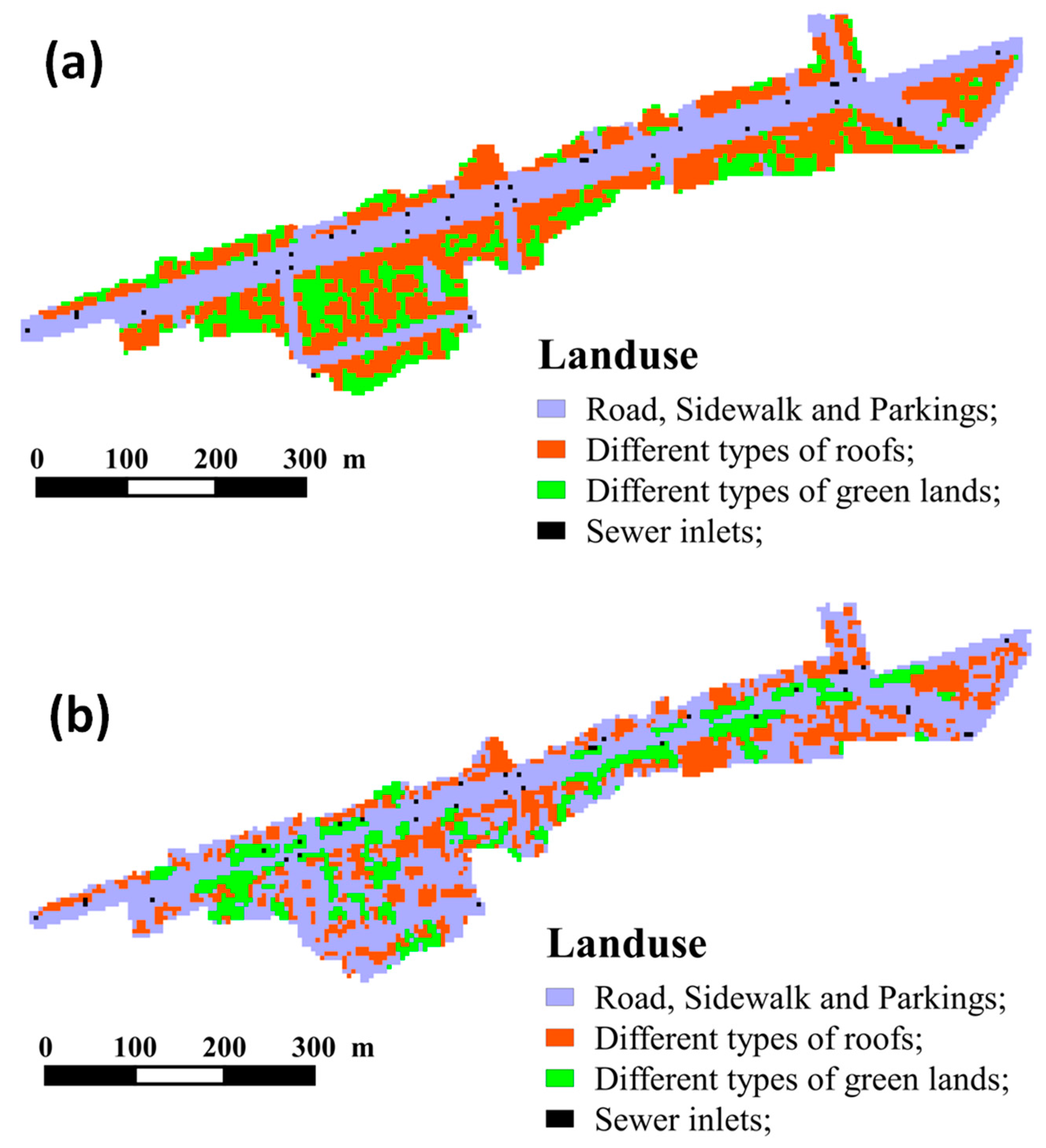
In the current study, we can benefit from detailed land use (LU) data which are derived from ortho-photos. In order to assess the model sensitivity to the fine knowledge of LU, we apply two simulation configurations: the first with detailed LU data derived from ortho-photos, and the second with regularly achieved LU data which contains only public buildings (stations, commercial centres, schools, etc.) and green-lands, the undefined areas are considered as the roads and parking. These two types of data are illustrated in
Figure 6. In general, the surface of urban roofs is largely underestimated with coarser LU information, while the road and parking surfaces are overestimated.
2.4.5. Scenario 5: Sensibility of the Water Quality Module to Different Particle Size Distributions (PSD)
For the water quality modelling, several stormwater samplings were performed at the outlet during rainfall events, and suspended solid measurements were then performed in the laboratory. Moreover, a series of road dust samples were collected on the studied urban surfaces using a 2 m
2 vacuum cleaner [
31]. This experiment was carried out on 14 October 2014 during dry weather after a dry period of 2 days. The measurements of the deposit samples could be used to calculate the total mass of road dust in the basin (2661 m
2), by supposing that the sediments are uniformly distributed on the road surface. Granulometric analysis was then conducted in the laboratory for evaluating the PSD of the studied samples. Based on the PSD and the total mass of each sample, we could calculate the mass of each particle size class. The mass and the particle size in different wet and dry samples are represented in
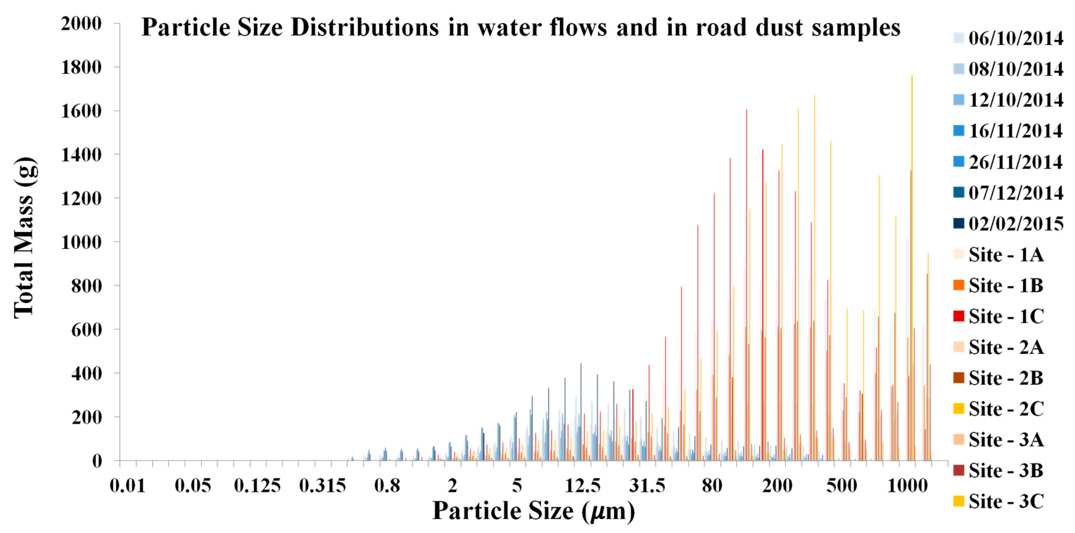
Figure 7.
In
Figure 7, we observe that PSD in stormwater samples are quite different from that in road dust samples, where fine particles (<100 μm) are major compositions (>90%) of Total Suspended Solids (TSS) in stormwater runoffs. Yet, it is contrary to the road dust samples (<10%). This phenomenon is caused by the fact that the finest particles of road dry deposits are transferred to the sewer network during typical rainfall events, whereas the coarser particles remain on the urban surface [
37]. Based on these measurements, we tested two configurations for assessing the sensitivity to the characteristics of the road surface sediments (
Table 4): (i) 3 particle classes based on dry deposit samples, which can represent all the available particles on the urban surfaces; (ii) 3 particle classes based on stormwater samples, which can only represent the removeable particles of the total dry stocks.
3. Results and Discussion
The results will be presented step by step in order to illustrate the influence of different factors on model outputs. To gain clarity in the following text, figures are only produced for the event of 15 November 2014. The results for all six studied events will be listed in the tables. The Root-Mean-Square-Error (RMSE) coefficient, Nash-Sutcliffe-Efficiency (NSE), and Mean-Root-Square-Deviation coefficient are used to evaluate the model performance. For assessing the model performance of different settings of model structures and input data, the most detailed configuration is considered as the benchmark reference. In fact, the double precision, the high resolution topographic data, and the detailed land use data are systematically used when one of them is analyzed. By altering different options of model configurations, the influence of different factors on model performance can be evaluated. The results of this research can help practitioners identify the key factors in 2D-1D modelling at the district scale in order to avoid the collection of unnecessary and costly data.
3.1. Scenario 1: Internal Numerical Precision of the Source Code
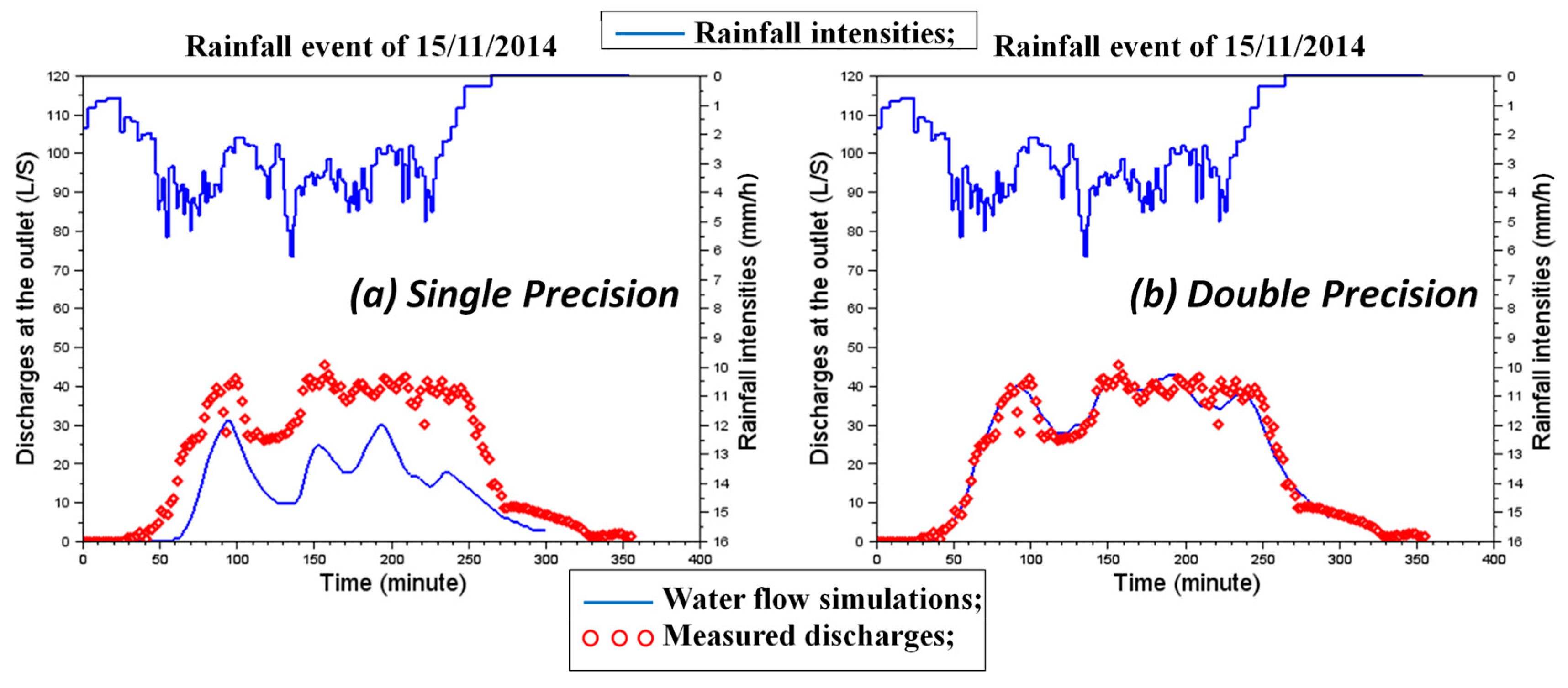
Figure 8 shows the change of the hydrograph in response to the change of digital precision (single-precision or double-precision floating point format) for the rainfall event of 15 November 2014, while the results of all rainfall events are presented in
Table 5.
As illustrated in
Figure 8 and
Table 5, simulations with single-precision floating-point format of the source code do not obtain acceptable results. Moreover, in practice, we have mentioned that, no matter what combinations of parameter values are taken, the dynamics of the simulation outputs are far from that of the measurements. As shown in
Figure 8, model outputs with single-precision floating-point format are more sensitive to the change in rainfall intensity. As precipitation in the Paris region usually consists of light rainfall (<10 mm/h), the accumulation of water volume in a grid cell (25 m
2) during a calculation time-step (0.1 s) is sometime less than 10
−7 cubic meters, especially at the beginning of the rainfall event. In that case, the volume of water is not represented during these time-steps with the single-precision floating-point format of the source code. While for the double-precision floating-point format of the source code, the internal numerical limit is 10
−14, this problem will not arise. In
Table 5, the results confirm that the model works well with the double-precision floating-point format of the source code. For these simulations, the distributed water quantity parameters are the “best-fit” parameters and the only change is the numerical precision of the source code. As can been seen in
Figure 8, the water balance is not conservative when the numerical precision is not appropriate. Therefore, the first step of urban stormwater modelling is to ensure that the water balance is correct, and the water quantity parameters can be adjusted at a later stage. For the current study, we will use the double-precision floating-point format in further evaluations as presented below.
3.2. Scenario 2: The Influence of the Calibration of Typical Model Parameters
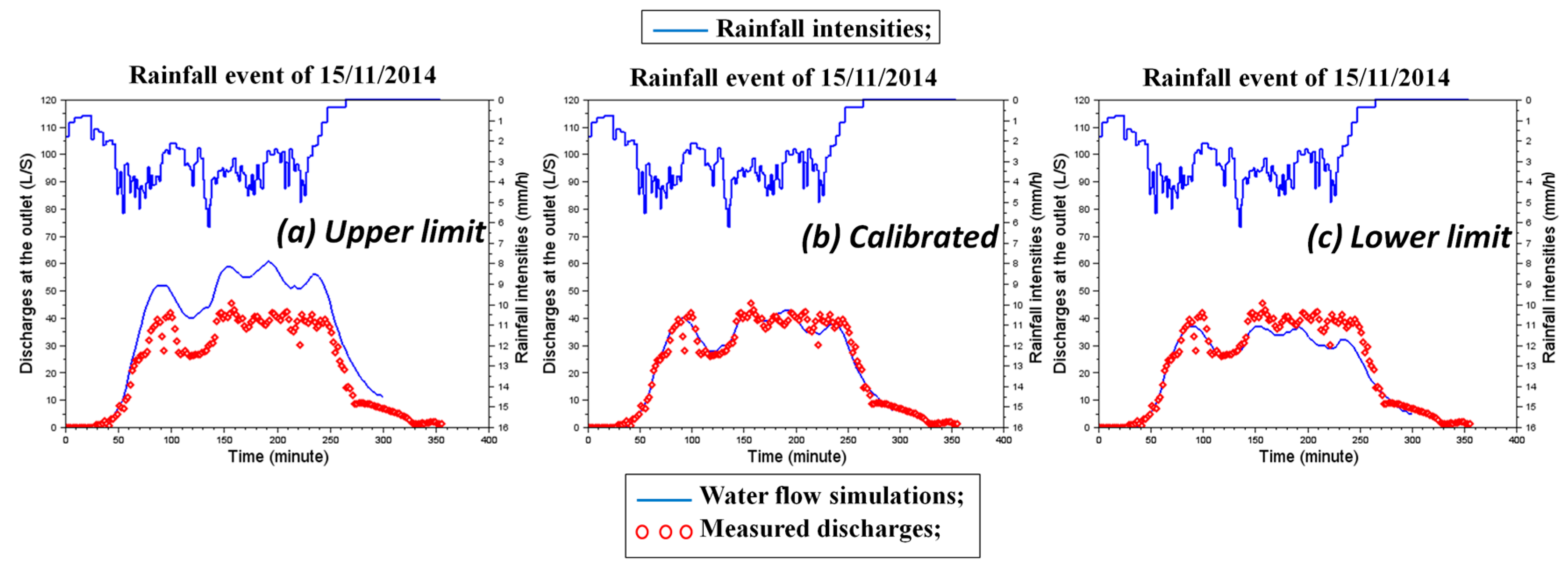
As presented in the above section, we test three model configurations by using Kh and surface flow Manning’s N value at their (i) upper limit; (ii) calibrated value and (iii) lower limit. The greatest Kh and Manning’s N values assume that the surface are more pervious and rough, while the lower limit of these two parameters means that the imperviousness of the urban land uses are much higher with smoother surfaces. The hydrograms of the event on 15 November 2014 are presented in
Figure 9, while the outcomes of all six events are illustrated in
Table 6.
Compared to the results of Scenario 1, simulations of Scenario 2 suggest that the impacts of parameters (Manning’s N, saturated hydraulic conductivity (Kh)) on model outputs are less significant than that of the numerical precision in source codes. The dynamics of simulated water flow and the model performance remain acceptable under different parameter configurations, particularly for the simulations using the lower limit of the parameter values. The physical properties of the two parameters can explain these results. The Manning’s equation is used to calculate the surface runoff velocity, since the studied urban catchment is relatively small (0.12 km
2) and the flow path from each grid cell to its nearest sewer inlet is short (less than 100 m). Surface runoffs can always rapidly enter the neighbouring sewer inlets regardless of the Manning’s N values. Besides, Kh is the essential parameter in the Green-Ampt model for infiltration modelling. It influences the total quantity of water entering the sewer system, but it has limited impact on flow dynamics. As shown in
Table 6, the simulated configurations for all six studied rainfall events display comparable results.
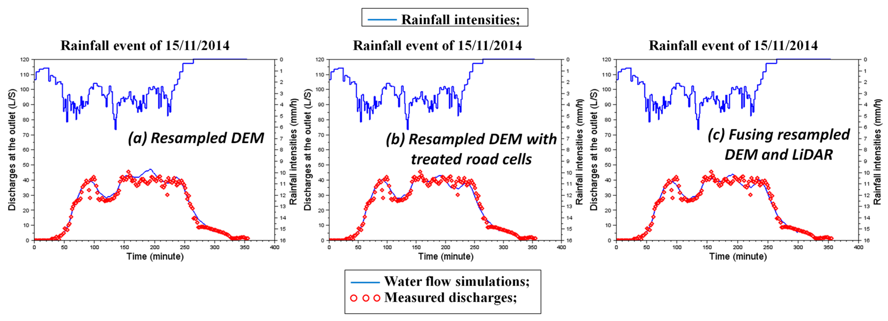
3.3. Scenario 3: Influence of the Road LiDAR Data in Comparison with DEM Data
In order to evaluate the impact of the merged high-resolution road LiDAR data, three different model configurations are established with different topographic input maps: (i) directly resampling the DEM data (25 m) to 5 m resolution; (ii) resampling the DEM data (25 m) to 5 m resolution, and then lowering the identified road grid cells by 20 cm; (iii) resampling the road LiDAR data (20 cm) and the DEM data (25 m) to 5 m resolution, then fusing the two types of data together. The simulation results are presented in
Figure 10 and
Table 7.
As can be seen in
Figure 10, it seems that the high resolution data on the road altimetry has a weak influence on model outputs. In
Table 7, the results confirm this observation for all six studied events, as model performance remains acceptable under different rainfall conditions. Moreover, simulations with DEM data with dug road appear to be slightly better than that only with DEM data, and they are similar in terms of performance to the model outputs with merged road LiDAR data and DEM data.
Since the major benefit of using high-resolution LiDAR data is to ensure that water flows in appropriate directions, the present study indicates that the flow directions in the TRENOE model are generally well represented even with coarser resolution topographic data. Therefore, we can conclude that using high resolution altimetry data is not a key factor for water flow simulations at the outlet of an urban catchment. Considering only basic topographic data with lower streets is sufficient for simulations.
3.4. Scenario 4: Influence of a Fine Knowledge of Land Use Based on Ortho-Photos
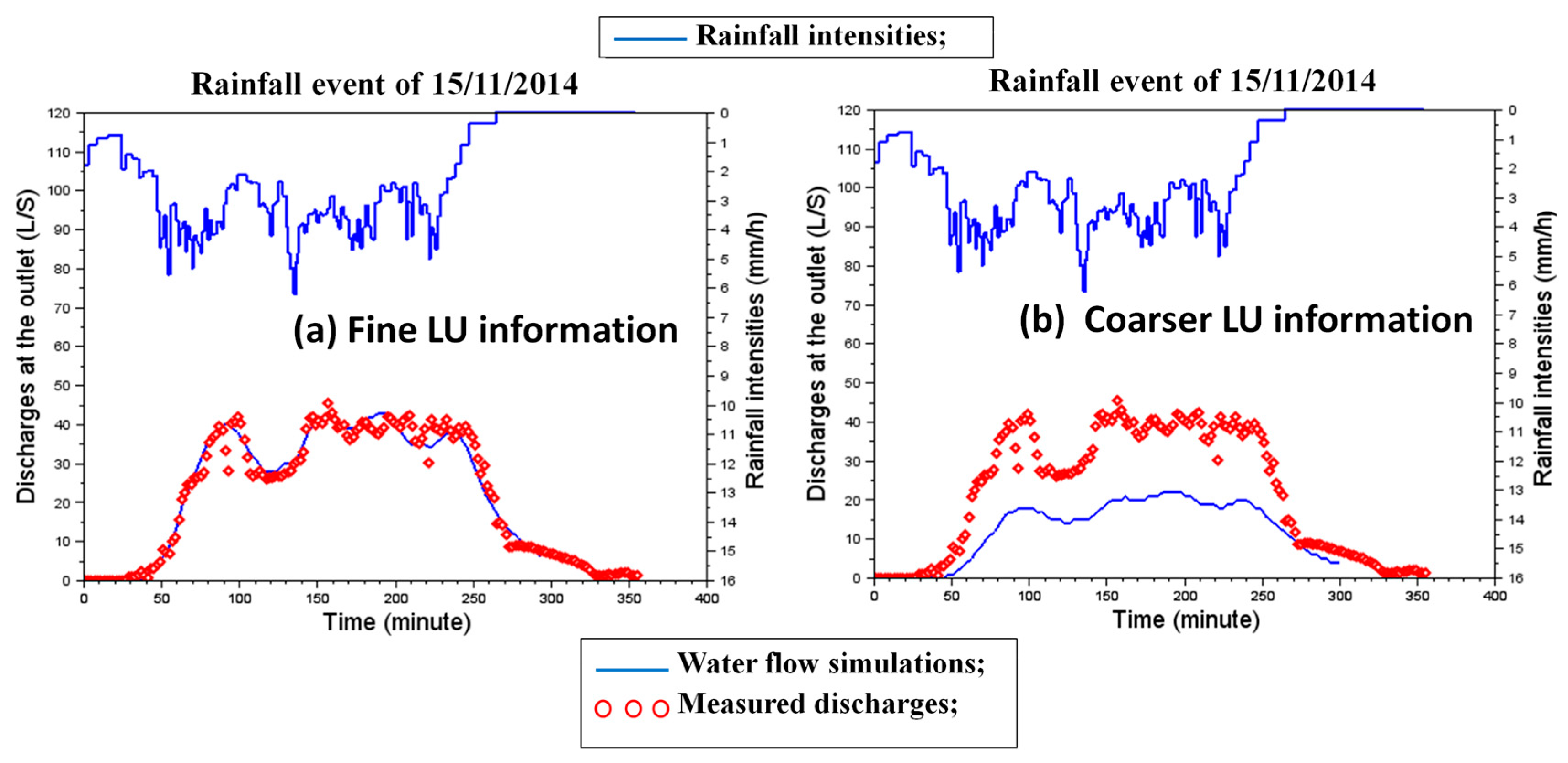
In collaboration with the French National Institute of Geography (IGN), detailed information on urban land use (LU) could be obtained. The vectorial land use data derived from the ortho photos can have a very high resolution even at the scale of centimetres, but transforming land use data into a reliable map of land uses is not straightforward. Because the urban environment is constituted of varied characteristics that have a typical size of less than 5 m (natural soil surrounding the trees next to the road, courtyards, etc.), and the analyses of the ortho photos are three dimensional. For example, the canopy has an extent on aerial photography which is not the land use at the ground level (in an urban catchment, this ground will be mainly pavement, for example). Therefore, when aggregating the land use classes at the scale of the mesh grid, it is very important to hierarchise the different land use types. The priority is based on the effect of the land use on the water quantity and quality. A specific priority between land uses has been defined for this transformation. In the current study, the priority land use is “sewer inlets”, followed by roads, sidewalks, parking lots, various types of roofs, trees, grass and others. As for the coarser LU information, the vectorial LU source data contains only public buildings and greenlands, and the undefined areas are considered as impermeable roads and parking areas. We followed the same priority order as mentioned before to generate LU input maps (5 m). The results of water flow simulation at the outlet of catchments using these two different LU input maps are presented in
Figure 11 and
Table 8.
As shown in
Figure 11, the simulation outputs with LU input map converted from coarser LU information do not match the measurements. In fact, the simulated water balance is far less than the observed one and the simulated hydrographs seem to be insensitive to the variations in rainfall intensity. Since private buildings are not included in the low resolution LU source data, the infiltration is overestimated and the longer pathways of surface runoff result in longer time of concentration compared with the water from roofs.
On the other hand, the results in
Table 8 indicate poor model performance with the input LU map converted from coarser LU information. This finding confirms that the land use information is an essential input data for this kind of urban stormwater 2D/1D modelling.
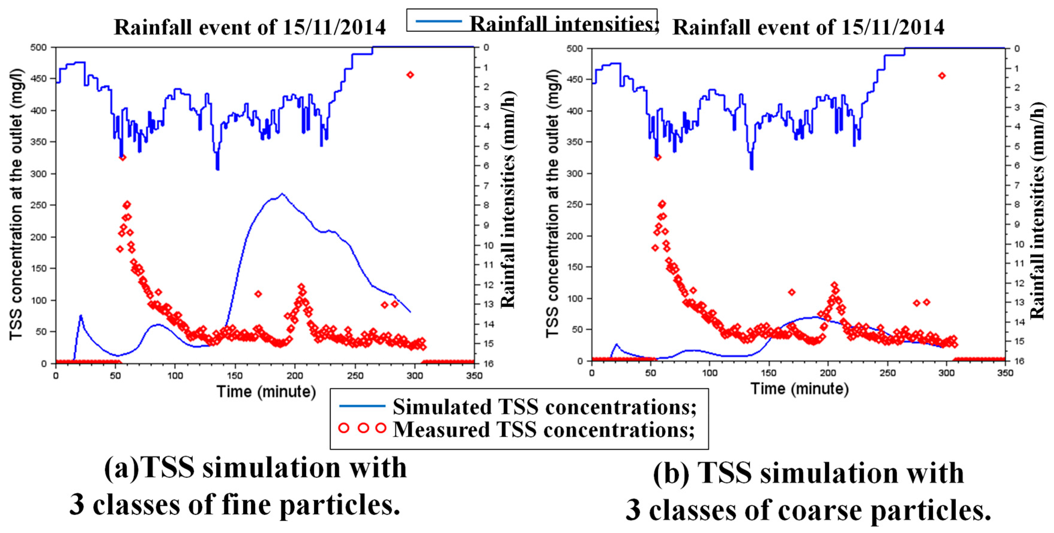
3.5. Scenario 5: Sensitivity of the Water Quality Module to Different Particle Size Distributions (PSD)
Since hydrological modelling is extensively discussed and calibrated in the above sections, we can now work on water quality simulations. As this is the first time that the USLE equation is adapted to an urban context, we fixed all the parameters to their maximum values which are equal to 1 in our first tests, including the rainfall erodibility factor (R), the soil erodibility factor (K), the topographic factors (L, S) and the cropping management factors (C, P). Because the PSD of stormwater samples are quite different from that of road dust samples (
Figure 7), we analyse the impact of different PSD values on water quality simulations in order to know which choice is appropriate for the current 2D/1D model. The simulation results are presented in
Figure 12.
According to
Figure 12, we can note that the simulations of Total Suspended Solids (TSS) concentrations vary across the configurations of the three classes of particles derived from PSD of stormwater samples (3.5 μm, 15 μm, 50 μm) and that derived from PSD of dry stock samples (7 μm, 70 μm, 250 μm). Since coarser particles have greater settling velocities, simulated TSS concentrations using three classes of fine particles are much higher than the other ones. Nevertheless, as with the classification based on fine particles or coarser particles, the water quality simulations are unsatisfactory with the current version of the TRENOE platform. It cannot reproduce the first peak of TSS concentration at the beginning of the rainfall event.
Indeed, the current code of TRENOE platform uses a modified form of Universal Soil Loss Equation (USLE) for simulating sediment erosion, where the pollutant wash-off from a given land use is represented as a mass rate of particle removal from the bottom boundary over time. Considering that the USLE method is originally designed to predict soil losses caused by runoff in agricultural areas, several adaptations are certainly needed to use it for urban areas, such as the alterations of USLE parameters according to different criterions, the definition of the appropriate initial dry deposits corresponding to various land uses, etc. Moreover, it is important to note that TRENOE does not include any detachment processes driven by raindrops, and the sediment erosion is only calculated from water flow detachment. Therefore, the actual version of TRENOE cannot simulate the first peak of TSS concentration when the water flow is still weak at the first part of the rainfall event. In agreement with the recent findings of [
37,
38] that the raindrop impacts are essential for wash off processes in urban areas, the raindrop-driven detachment should be taken into account for further studies.
4. Conclusion and Perspectives
In this study, we describe an attempt to develop an integrated 2D/1D modelling platform “TRENOE”, as well as the necessary modelling assumptions and adaptations to simulate both quantitative and qualitative hydrological processes for urban areas. The physically-based combined modelling system is established for water flow and water quality modelling by coupling urban surface and sewer networks.
Within the framework of the ANR (French National Agency for Research) Trafipollu project, TRENOE platform is applied to a small urban catchment near Paris (Le Perreux sur Marne, 0.12 km2). In collaboration with other partners within the project, high-resolution topographic data from LiDAR survey, detailed land use data derived from ortho-photos, and Particle Size Distributions (PSD) are obtained for the studied urban catchment. Benefitting from these elaborate sources of input data, this article tests the relative influence of various factors on the outputs of the model, particularly the influence of numerical precision on source code, the influence of common parameters on water quality, and the influence of having precise knowledge of the topography (more or less known with great precision) and land uses. By analysing the impacts of these internal and external factors on model outputs, the main objective of this work is hence not only to identify which factors are significant for urban 2D/1D stormwater modelling, because all of them are, but mainly to underline the necessary model configurations for appropriate simulations with limited availability of data sources and human modelling and simulation capabilities.
The numerical precision of source codes and the precise knowledge of land uses are proved to be the most influential factors in the model outputs, whereas the resolution of road topographic data and the model parameters have less impact. These findings can assist urban stormwater managers in better organising their efforts in data surveys to improve model accuracy from necessary field investigations. Besides, the present results emphasise the importance of considering the parameters’ physical significance in the model calibration. In cases where the dynamics of model outputs greatly differ from measurements and cannot be explained by the effects of parameters, there may be internal issues with the model or problems with input data. Of course, these results need to be confirmed by applying this modelling approach to other urban catchments with different shapes and slopes.
Concerning water quality modelling, the present work fails to correctly reproduce the concentration of Total-Suspended-Solids (TSS) at the catchment outlet. However, the importance of taking into account the appropriate particle classification is highlighted. Using only empirical USLE equations is certainly responsible for the poor performance of the sediment erosion modelling. Taking into account the direct detachment by rain drops is essential for improving urban stormwater quality modelling. Testing the robustness of our main observations of an urban catchment showing different physical characteristics (larger, steeper, with more green spaces etc.) would also represent an interesting perspective in the future.
Acknowledgments
The research work of Ph.D. student Yi Hong was financed by ANR-Trafipollu project (ANR-12-VBDU-0002) and Ecole des Ponts ParisTech. Firstly, the authors would like to thank OPUR (Observatoire des Polluants Urbains en Ile-de-France) for providing the platform for changing idears and elaborating collaborations with diffrent researchers from various institutions. The authors would also like to thank B. Béchet (IFSTTAR), B. Soleilhan (IGN) and V. Bousquet (IGN-Conseil) for providing invaluable measurements and GIS data. We also want to give a special thanks to the experimental team of ANR Trafipollu project for all collected necessary for this work, in particular David Ramier (CEREMA), Mohamed Saad (LEESU) and Philippe Dubois (LEESU).
Author Contributions
This study was designed by Yi Hong, Céline Bonhomme and Ghassan Chebbo. The manuscript was prepared by Yi Hong and revised by Céline Bonhomme and Ghassan Chebbo.
Conflicts of Interest
The authors declare no conflict of interest.
References
- Walsh, C.J.; Fletcher, T.D.; Ladson, A.R. Stream restoration in urban catchments through redesigning stormwater systems: Looking to the catchment to save the stream. J. N. Am. Benthol. Soc. 2005, 24, 690–705. [Google Scholar] [CrossRef]
- Deffontis, S.; Breton, A.; Vialle, C.; Montréjaud-Vignoles, M.; Vignoles, C.; Sablayrolles, C. Impact of dry weather discharges on annual pollution from a separate storm sewer in Toulouse, France. Sci. Total Environ. 2013, 452–453, 394–403. [Google Scholar] [CrossRef] [PubMed] [Green Version]
- Bressy, A.; Gromaire, M.-C.; Lorgeoux, C.; Saad, M.; Leroy, F.; Chebbo, G. Efficiency of source control systems for reducing runoff pollutant loads: Feedback on experimental catchments within Paris conurbation. Water Res. 2014, 57, 234–246. [Google Scholar] [CrossRef] [PubMed] [Green Version]
- Hatt, B.E.; Fletcher, T.D.; Walsh, C.J.; Taylor, S.L. The influence of urban density and drainage infrastructure on the concentrations and loads of pollutants in small streams. Environ. Manag. 2004, 34, 112–124. [Google Scholar] [CrossRef] [PubMed]
- Clark, S.; Pitt, R.; Burian, S.; Field, R.; Fan, E.; Heaney, J.; Wright, L. Annotated Bibliography of Urban Wet Weather Flow Literature from 1996 through 2006; Environmental Engineering Program: Middleton, PA, USA, 2007. [Google Scholar]
- Duncan, H. A Review of Urban Stormwater Quality Processes; Report 95/9 for Cooperative Research Centre for Catchment Hydrology: Clayton, Australia, 1995. [Google Scholar]
- Vaze, J.; Chiew, F.H.S. Comparative evaluation of urban storm water quality models. Water Resour. Res. 2003, 39, 1280. [Google Scholar] [CrossRef]
- Rossman, L.A. Storm Water Management Model User’s Manual Version 5.0; National Risk Management Research and Development, U.S. Environmental Protection Agency: Cincinnati, OH, USA, 2010.
- Wong, T.H.F.; Fletcher, T.D.; Duncan, H.P.; Coleman, J.R.; Jenkins, G.A. A Model for Urban Stormwater Improvement: Conceptualization; American Society of Civil Engineers: Portland, OR, USA, 2002; pp. 1–14. [Google Scholar]
- Elliott, A.H.; Trowsdale, S.A. A review of models for low impact urban stormwater drainage. Environ. Model. Softw. 2007, 22, 394–405. [Google Scholar] [CrossRef]
- Sartor, J.D.; Boyd, G.B.; Agardy, F.J. Water pollution aspects of street surface contaminants. J. Water Pollut. Control Fed. 1974, 46, 458–467. [Google Scholar] [PubMed]
- Bonhomme, C.; Petrucci, G. Spatial representation in semi-distributed modelling of water quantity and quality. In Proceedings of the 13th International Conference on Urban Drainage, Kuching, Malaysia, 7–11 September 2014.
- Kanso, A. Evaluation des Modeles de Calcul des Flux Polluants des Rejets Urbains par Temps de Pluie. Apport de L’Approche Bayesienne. Ph.D. Thesis, Ecole Nationale des Ponts et Chaussées, Champs-sur-Marne, France, 22 September 2004. [Google Scholar]
- Sage, J.; Bonhomme, C.; Al Ali, S.; Gromaire, M.-C. Performance assessment of a commonly used “accumulation and wash-off” model from long-term continuous road runoff turbidity measurements. Water Res. 2015, 78, 47–59. [Google Scholar] [CrossRef] [PubMed] [Green Version]
- Bach, P.M.; Rauch, W.; Mikkelsen, P.S.; McCarthy, D.T.; Deletic, A. A critical review of integrated urban water modelling—Urban drainage and beyond. Environ. Model. Softw. 2014, 54, 88–107. [Google Scholar] [CrossRef]
- Vojinovic, Z.; Tutulic, D. On the use of 1D and coupled 1D-2D modelling approaches for assessment of flood damage in urban areas. Urban Water J. 2009, 6, 183–199. [Google Scholar] [CrossRef]
- Chen, A.S.; Djordjevic, S.; Leandro, J.; Savic, D. The urban inundation model with bidirectional flow interaction between 2D overland surface and 1D sewer networks. In Proceedings of the NOVATECH 2007—Sixth International Conference on Sustainable Techniques and Strategies in Urban Water Management, Lyon, Rhone-Alpes, France, 25–28 June 2007; pp. 465–472.
- Djordjević, S.; Prodanović, D.; Maksimović, C.; Ivetić, M.; Savić, D. SIPSON—Simulation of interaction between pipe flow and surface overland flow in networks. Water Sci. Technol. 2005, 52, 275–283. [Google Scholar] [PubMed]
- Kidmose, J.; Troldborg, L.; Refsgaard, J.C.; Bischoff, N. Coupling of a distributed hydrological model with an urban storm water model for impact analysis of forced infiltration. J. Hydrol. 2015, 525, 506–520. [Google Scholar] [CrossRef]
- Domingo, N.D.S.; Refsgaard, A.; Mark, O.; Paludan, B. Flood analysis in mixed-urban areas reflecting interactions with the complete water cycle through coupled hydrologic-hydraulic modelling. Water Sci. Technol. 2010, 62, 1386–1392. [Google Scholar] [CrossRef] [PubMed]
- DHI MIKE by DHI Software. Reference Manuals for MIKE FLOOD. 2008. Available online: https://www.mikepoweredbydhi.com/products/mike-flood (accessed on 19 December 2016).
- Innovyze Ltd. InfoWorks 2D-Collection Systems Technical Review. 2011. Available online: http://www.innovyze.com/products/infoworks_cs/infoworks_2d.aspx (accessed on 19 December 2016).
- McMichael, C.E.; Hope, A.S.; Loaiciga, H.A. Distributed hydrological modelling in California semi-arid shrublands: MIKE SHE model calibration and uncertainty estimation. J. Hydrol. 2006, 317, 307–324. [Google Scholar] [CrossRef]
- Thompson, J.R.; Sørenson, H.R.; Gavin, H.; Refsgaard, A. Application of the coupled MIKE SHE/MIKE 11 modelling system to a lowland wet grassland in southeast England. J. Hydrol. 2004, 293, 151–179. [Google Scholar] [CrossRef]
- Velleux, M.L. Spatially Distributed Model to Assess Watershed Contaminant Transport and Fate. Ph.D. Thesis, Colorado State University, Fort Collins, CO, USA, 2005. [Google Scholar]
- Velleux, M.L.; England, J.F.; Julien, P.Y. TREX: Spatially distributed model to assess watershed contaminant transport and fate. Sci. Total Environ. 2008, 404, 113–128. [Google Scholar] [CrossRef] [PubMed]
- Lhomme, J.; Bouvier, C.; Perrin, J.-L. Applying a GIS-based geomorphological routing model in urban catchments. J. Hydrol. 2004, 299, 203–216. [Google Scholar] [CrossRef]
- Cheng, N.-S. Simplified settling velocity formula for sediment particle. J. Hydraul. Eng. 1997, 123, 149–152. [Google Scholar] [CrossRef]
- Gallegos, H.A.; Schubert, J.E.; Sanders, B.F. Two-dimensional, high-resolution modeling of urban dam-break flooding: A case study of Baldwin Hills, California. Adv. Water Resour. 2009, 32, 1323–1335. [Google Scholar] [CrossRef]
- Fewtrell, T.J.; Duncan, A.; Sampson, C.C.; Neal, J.C.; Bates, P.D. Benchmarking urban flood models of varying complexity and scale using high resolution terrestrial LiDAR data. Phys. Chem. Earth ABC 2011, 36, 281–291. [Google Scholar] [CrossRef]
- Bechet, B.; Bonhomme, C.; Lamprea, K.; Campos, E.; Jean-soro, L.; Dubois, P.; Lherm, D. Towards a modeling of pollutant flux at local scale—Chemical analysis and micro-characterization of road dusts. In Presented at the 12th Urban Environment Symposium, Oslo, Norway, 1–3 June 2015.
- Nash, J.E.; Sutcliffe, J.V. River flow forecasting through conceptual models part I—A discussion of principles. J. Hydrol. 1970, 10, 282–290. [Google Scholar] [CrossRef]
- England, J.F.; Julien, P.Y.; Velleux, M.L. Physically-based extreme flood frequency with stochastic storm transposition and paleoflood data on large watersheds. J. Hydrol. 2014, 510, 228–245. [Google Scholar] [CrossRef]
- Ayvaz, M.T. A linked simulation–optimization model for simultaneously estimating the Manning’s surface roughness values and their parameter structures in shallow water flows. J. Hydrol. 2013, 500, 183–199. [Google Scholar] [CrossRef]
- Butler, T.; Graham, L.; Estep, D.; Dawson, C.; Westerink, J.J. Definition and solution of a stochastic inverse problem for the Manning’s n parameter field in hydrodynamic models. Adv. Water Resour. 2015, 78, 60–79. [Google Scholar] [CrossRef] [PubMed]
- Coustau, M.; Rousset-Regimbeau, F.; Thirel, G.; Habets, F.; Janet, B.; Martin, E.; de Saint-Aubin, C.; Soubeyroux, J.-M. Impact of improved meteorological forcing, profile of soil hydraulic conductivity and data assimilation on an operational Hydrological Ensemble Forecast System over France. J. Hydrol. 2015, 525, 781–792. [Google Scholar] [CrossRef]
- Hong, Y.; Bonhomme, C.; Le, M.-H.; Chebbo, G. A new approach of monitoring and physically-based modelling to investigate urban wash-off process on a road catchment near Paris. Water Res. 2016, 102, 96–108. [Google Scholar] [CrossRef] [PubMed]
- Hong, Y.; Bonhomme, C.; Le, M.-H.; Chebbo, G. New insights into the urban washoff process with detailed physical modelling. Sci. Total Environ. 2016, 573, 924–936. [Google Scholar] [CrossRef] [PubMed]
Figure 1.
The scheme of the physically-based 2D/1D modelling platform TRENOE.
Figure 1.
The scheme of the physically-based 2D/1D modelling platform TRENOE.
Figure 2.
Delineated urban catchment of the study site, Le Perreux-sur-Marne, France.
Figure 2.
Delineated urban catchment of the study site, Le Perreux-sur-Marne, France.
Figure 3.
Histogram of rainfall event characteristics over the entire period: (a) rainfall depth; (b) mean intensity; (c) event duration; and (d) antecedent dry days.
Figure 3.
Histogram of rainfall event characteristics over the entire period: (a) rainfall depth; (b) mean intensity; (c) event duration; and (d) antecedent dry days.
Figure 4.
Topographic input data. (a) DEM data of 25 m resolution; (b) Roads LiDAR data of 20 cm resolution; (c) Merged topographic input data of 5 m resolution.
Figure 4.
Topographic input data. (a) DEM data of 25 m resolution; (b) Roads LiDAR data of 20 cm resolution; (c) Merged topographic input data of 5 m resolution.
Figure 5.
Input data for TRENOE: (a) separate stormwater sewer networks; (b) vectorial land use data; (c) raster land use data with 5 m resolution.
Figure 5.
Input data for TRENOE: (a) separate stormwater sewer networks; (b) vectorial land use data; (c) raster land use data with 5 m resolution.
Figure 6.
Land use (LU) input map (5 m) converted from different data sources: (a) from the detailed LU information which is derived from ortho photos; (b) from the coarser LU information which is used for urban planning.
Figure 6.
Land use (LU) input map (5 m) converted from different data sources: (a) from the detailed LU information which is derived from ortho photos; (b) from the coarser LU information which is used for urban planning.
Figure 7.
Particle Size Distributions of stormwater samples (blue bars) and road dust samples (yellow bars) during a dry weather sampling campaign (14 October 2014).
Figure 7.
Particle Size Distributions of stormwater samples (blue bars) and road dust samples (yellow bars) during a dry weather sampling campaign (14 October 2014).
Figure 8.
Change of the hydrograph due to the change from (a) single-precision to (b) double-precision floating-point format of the source code. The simulated discharges at the outlet (solid blue line) are compared with the measured data (red circles). Rainfall is plotted on the upper part.
Figure 8.
Change of the hydrograph due to the change from (a) single-precision to (b) double-precision floating-point format of the source code. The simulated discharges at the outlet (solid blue line) are compared with the measured data (red circles). Rainfall is plotted on the upper part.
Figure 9.
Hydrogram at the outlet of catchment using different values of water flow parameters. For (a) simulation using the upper limits of the parameter values; (b) simulation using the calibrated parameter values; (c) simulation using the lower limit of the parameter values. The simulated discharges at the outlet (solid blue line) are compared with the measured data (red circles). Rainfall is plotted on the upper part.
Figure 10.
Hydrographs at the outlet of catchment using different topographic input maps. For (a) directly resampling the DEM data (25 m) to 5 m resolution; (b) resampling the DEM data (25 m) to 5 m resolution, and then lowering the identified road grid cells by 20 cm; (c) resampling the road LiDAR data (20 cm) and the DEM data (25 m) to 5 m resolution, then fusing the two types of data together. The simulated discharges at the outlet (solid blue line) are compared with the measured data (red circles). Rainfall is plotted on the upper part.
Figure 11.
Hydrogram at the outlet of catchment using different land use (LU) input maps. For (a) LU input map (5 m) converted from fine LU information; (b) LU input map (5 m) converted from coarser LU information. The simulated discharges at the outlet (solid blue line) are compared with the measured data (red circles). Rainfall is plotted on the upper part.
Figure 12.
Water quality simulations with different Particle Size Distributions for (a) three classes of fine particles derived from PSD of stormwater samples: 3.5 μm, 15 μm, 50 μm; (b) three classes of coarse particles derived from PSD of dry stock samples: 7 μm, 70 μm, 250 μm. The simulated TSS concentrations at the outlet (solid blue line) are compared with the measured data (red circles). Rainfall is plotted on the upper part.
Table 1.
Modelling processes in the 2D/1D TRENOE platform.
Table 1.
Modelling processes in the 2D/1D TRENOE platform.
| Modelling Process | 2D Overland Modelling: TREX | Conceptual Roofs Modelling: CANOE | 1D Sewer Network Modelling: CANOE |
|---|
| Water flow | 2D Shallow-Water equations; (Diffusive Wave) | Non-linear reservoir | 1D Shallow-Water equations; (Kinematic Wave) |
| Infiltration | Green & Ampt | - | - |
| Interception | Volume loss | - | - |
| Sediment deposition | Settling velocity [28] | - | - |
| Sediment erosion | Modified form of Universal Soil Loss Equation (USLE) | Exponential washoff equations | - |
| Numerical method | Finite Difference | Finite Difference | Finite Difference |
Table 2.
Summary of the 6 selected rainfall events.
Table 2.
Summary of the 6 selected rainfall events.
| Rainfall Date | Rainfall Depth (mm) | Mean Intensity (mm/h) | Duration (h) | Antecedent Dry Days (Day) |
|---|
| 8 October 2014 | 4.86 | 1.51 | 3.22 | 0.4 |
| 12 October 2014 | 3.60 | 1.68 | 2.14 | 1.3 |
| 3 November 2014 | 4.6 | 1.33 | 3.46 | 12.9 |
| 15 November 2014 | 9.27 | 2.81 | 3.3 | 0.5 |
| 26 November 2014 | 2.86 | 1.1 | 2.6 | 9 |
| 12 December 2014 | 4.15 | 1.28 | 3.24 | 2.5 |
Table 3.
Different configurations of saturated hydraulic conductivity (Kh) and Manning’s N coefficient for Scenario 2 simulations.
Table 3.
Different configurations of saturated hydraulic conductivity (Kh) and Manning’s N coefficient for Scenario 2 simulations.
| Parameters | N-Manning | Kh (m/s) |
|---|
| Landuse | Roads | Green-lands | Roads | Green-lands |
| Upper limits of parameters | 0.02 | 0.05 | 1 × 10⁻⁷ | 1 × 10⁻⁴ |
| Calibrated Parameters | 0.015 | 0.03 | 1 × 10⁻⁸ | 1 × 10⁻⁵ |
| Lower limits parameters | 0.01 | 0.02 | 1 × 10⁻¹⁰ | 1 × 10⁻⁷ |
Table 4.
Two configurations of different particle size classifications.
Table 4.
Two configurations of different particle size classifications.
| Particle Size (μm) | Median Diameter (μm) | Percentage | Settling Velocity (cm/s) |
|---|
| Configuration 1, based on road dry deposit samples |
| <15 | 7 | 10% | 0.002 |
| 15–125 | 70 | 40% | 1.92 |
| >125 | 250 | 50% | 1.78 |
| Configuration 2, based on stormwater runoff samples |
| <7 | 3.5 | 30% | 0.0005 |
| 7–25 | 15 | 40% | 0.009 |
| >25 | 50 | 30% | 0.1 |
Table 5.
Influence of numerical precision of the source codes on water flow at the outlet of the sewer system.
Table 5.
Influence of numerical precision of the source codes on water flow at the outlet of the sewer system.
| Date | NSE | RMSE | MRSD |
|---|
| Double | Single | Double | Single | Double | Single |
|---|
| 8 October 2014 | 0.88 | 0.09 | 5.9 | 16.9 | 0.39 | 0.78 |
| 12 October 2014 | 0.89 | 0.41 | 3.21 | 7.48 | 0.54 | 0.82 |
| 3 November 2014 | 0.89 | 0.67 | 7.74 | 13.32 | 0.38 | 0.64 |
| 15 November 2014 | 0.97 | 0.06 | 2.69 | 14.7 | 0.14 | 0.53 |
| 26 November 2014 | 0.76 | 0.14 | 5.08 | 9.67 | 0.59 | 1.29 |
| 12 December 2014 | 0.28 | −0.16 | 21.33 | 27.3 | 0.27 | 0.51 |
Table 6.
Influences of parameter values on water flow at the outlet of the sewer system.
Table 6.
Influences of parameter values on water flow at the outlet of the sewer system.
| Date | NSE | RMSE | MRSD |
|---|
| Calibrated | Lower Limit | Upper Limit | Calibrated | Lower Limit | Upper Limit | Calibrated | Lower Limit | Upper Limit |
|---|
| 8 October 2014 | 0.88 | 0.79 | 0.52 | 5.9 | 8.83 | 12.43 | 0.39 | 0.45 | 0.5 |
| 12 October 2014 | 0.89 | 0.78 | 0.33 | 3.21 | 5.12 | 9.43 | 0.54 | 0.68 | 0.72 |
| 3 November 2014 | 0.89 | 0.8 | 0.45 | 7.74 | 10.23 | 17.25 | 0.38 | 0.42 | 0.51 |
| 15 November 2014 | 0.97 | 0.9 | 0.19 | 2.69 | 4.67 | 13.6 | 0.14 | 0.18 | 0.46 |
| 26 November 2014 | 0.76 | 0.61 | 0.52 | 5.08 | 6.21 | 13.18 | 0.59 | 0.62 | 0.66 |
| 12 December 2014 | 0.28 | 0.15 | 0.16 | 21.33 | 23.12 | 23.54 | 0.27 | 0.31 | 0.32 |
Table 7.
Influence of high-resolution road topographic data on water flow at the outlet of the sewer system.
Table 7.
Influence of high-resolution road topographic data on water flow at the outlet of the sewer system.
| Date | NSE | RMSE | MRSD |
|---|
| Fusing Resampled DEM and LiDAR | Resampled DEM | Resampled DEM with Dug Roads | Fusing Resampled DEM and LiDAR | Resampled DEM | Resampled DEM with Dug Roads | Fusing Resampled DEM and LiDAR | Resampled DEM | Resampled DEM with Dug Roads |
|---|
| 8 October 2014 | 0.88 | 0.85 | 0.87 | 5.9 | 6.14 | 6.04 | 0.39 | 0.42 | 0.4 |
| 12 October 2014 | 0.89 | 0.8 | 0.83 | 3.21 | 4.01 | 3.87 | 0.54 | 0.6 | 0.58 |
| 3 November 2014 | 0.89 | 0.78 | 0.8 | 7.74 | 9.04 | 8.55 | 0.38 | 0.49 | 0.44 |
| 15 November 2014 | 0.97 | 0.9 | 0.89 | 2.69 | 2.94 | 2.78 | 0.14 | 0.18 | 0.15 |
| 26 November 2014 | 0.76 | 0.7 | 0.71 | 5.08 | 6.12 | 5.66 | 0.59 | 0.65 | 0.62 |
| 12 December 2014 | 0.28 | 0.25 | 0.26 | 21.33 | 23.01 | 22.11 | 0.27 | 0.33 | 0.3 |
Table 8.
Influence of fine land use (LU) information on water flow at the outlet of the sewer system.
Table 8.
Influence of fine land use (LU) information on water flow at the outlet of the sewer system.
| Date | NSE | RMSE | MRSD |
|---|
| Fine LU Information | Coarser LU Information | Fine LU Information | Coarser LU Information | Fine LU Information | Coarser LU Information |
|---|
| 8 October 2014 | 0.88 | 0.16 | 5.9 | 16.14 | 0.39 | 0.65 |
| 12 October 2014 | 0.89 | 0.21 | 3.21 | 12.37 | 0.54 | 0.88 |
| 3 November 2014 | 0.89 | 0.14 | 7.74 | 21.2 | 0.38 | 0.67 |
| 15 November 2014 | 0.97 | 0.04 | 2.69 | 14.9 | 0.14 | 0.5 |
| 26 November 2014 | 0.76 | 0.07 | 5.08 | 19.67 | 0.59 | 0.87 |
| 12 December 2014 | 0.28 | −0.5 | 21.33 | 32.1 | 0.27 | 0.42 |
© 2016 by the authors; licensee MDPI, Basel, Switzerland. This article is an open access article distributed under the terms and conditions of the Creative Commons Attribution (CC-BY) license (http://creativecommons.org/licenses/by/4.0/).


