Article

Analysis of Potential Future Climate and Climate Extremes in the Brazos Headwaters Basin, Texas

College of Agriculture and Human Sciences, Prairie View A&M University, Prairie View, TX 77446, USA
*
Author to whom correspondence should be addressed.
Water 2016, 8(12), 603; https://doi.org/10.3390/w8120603
Submission received: 5 August 2016 / Revised: 23 November 2016 / Accepted: 13 December 2016 / Published: 20 December 2016
(This article belongs to the Special Issue Land Use, Climate, and Water Resources)

Abstract

:
Texas’ fast-growing economy and population, coupled with cycles of droughts due to climate change, are creating an insatiable demand for water and an increasing need to understand the potential impacts of future climates and climate extremes on the state’s water resources. The objective of this study was to determine potential future climates and climate extremes; and to assess spatial and temporal changes in precipitation (Prec), and minimum and maximum temperature (Tmin and Tmax, respectively), in the Brazos Headwaters Basin under three greenhouse gas emissions scenarios (A2, A1B, and B1) for three future periods: 2020s (2011–2030), 2055s (2046–2065), and 2090s (2080–2099). Daily gridded climate data obtained from Climate Forecast System Reanalysis (CFSR) were used to downscale outputs from 15 General Circulation Models (GCMs) using the Long Ashton Research Station–Weather Generator (LARS-WG) model. Results indicate that basin average Tmin and Tmax will increase; however, annual precipitation will decrease for all periods. Annual precipitation will decrease by up to 5.2% and 6.8% in the 2055s and 2090s, respectively. However, in some locations in the basin, up to a 14% decrease in precipitation is projected in the 2090s under the A2 (high) emissions scenario. Overall, the northwestern and southern part of the Brazos Headwaters Basin will experience greater decreases in precipitation. Moreover, precipitation indices of the number of wet days (prec ≥ 5 mm) and heavy precipitation days (prec ≥ 10 mm) are projected to slightly decrease for all future periods. On the other hand, Tmin and Tmax will increase by 2 and 3 °C on average in the 2055s and 2090s, respectively. Mostly, projected increases in Tmin and Tmax will be in the upper range in the southern and southeastern part of the basin. Temperature indices of frost (Tmin < 0 °C) and ice days (Tmax < 0 °C) are projected to decrease, while tropical nights (Tmin > 20 °C) and summer days (Tmax > 25 °C) are expected to increase. However, while the frequency distribution of meteorological drought shows slight shifts towards the dry range, there was no significant difference between the baseline and projected meteorological drought frequency and severity.

1. Introduction

Climate change poses serious risks to the environment and human livelihood [1,2]. With anticipated changes in climate and increased climate variability, severe droughts and recurrent floods are becoming more frequent throughout the world [3]. Projected increases in climate extremes (e.g., heat waves and severe snowstorms) are expected to result in serious health problems [1,4,5]. The hydrologic cycle is adversely affected by climate change, especially shifts in spatial and temporal rainfall distribution and intensity [6,7]. In addition, climate change and climate variability have been causing significant shifts in frequency and intensity of climate extremes, e.g., minimum and maximum temperatures [8,9] and droughts [10,11,12]. Climate extremes, e.g., droughts and floods, disrupt agricultural and ecosystem processes [12,13].
Texas’ economic and population growth, combined with cycles of droughts and uncertainty due to climate change, are creating an increasingly unquenchable demand for water. In order for Texas to sustain its current and future economic growth, there is a need to better understand how potential future climates and climate extremes would affect the environment and water resources in the near, mid, and long-term future periods (2020s, 2055s, and 2090s, respectively).
Studies on potential climate changes and extreme events heavily relied on numerical modeling based on data generated from different General Circulation Models (GCMs) that provide useful information on the projections of future global climate [14,15,16,17]. However, GCMs outputs are available at coarse spatial resolutions, e.g., temperature and precipitation predictions at large grids (~100 by 100 km) [17,18]. Thus, downscaling of these GCMs outputs to finer resolutions has been widely implemented for local-scale climate impact studies [14,19] to provide needed data for different stakeholders to make informed adaptation and mitigation decisions. Such data are also useful in understanding the potential changes in available water resources and subsequently to assess their impact on major water users (e.g., agriculture, domestic, industries, and ecosystems).
Downscaling of GCMs outputs is mostly done using either statistical or dynamical approaches [20,21,22,23,24], which are widely used to downscale monthly GCMs’ temperature and rainfall projections to daily values for a specific location of interest at higher resolutions [23]. The statistical downscaling approach develops statistical relationships between local climate variables (e.g., temperature and precipitation) and large-scale predictors (e.g., pressure patterns), and applies this relationship to GCM outputs for future periods. Wilby and Wigely [24] classified statistical downscaling approaches into three groups: regression methods, weather pattern-based approaches, and stochastic weather generators. The latter is implemented in the LARS-WG model, which employs a stochastic weather generator approach [21,25]. The dynamical downscaling approach, however, uses higher resolution regional climate models (RCMs) nested into GCMs that better represent climates of smaller areas of interest, but require greater computational capabilities [25]. The statistical downscaling approach, on the other hand, is simple and easy, and could be performed using ordinary computers. However, it also has some major drawbacks. The major limitation of the statistical downscaling approach is that it assumes the statistical relationship between the historical climate and GCMs will remain stationary for future periods under climate change [24,26,27]. Details of the limitations and strengths of the dynamical and statistical downscaling approaches are discussed in detail by Wilby and Wigely [24].
Several studies [6,28,29,30,31,32,33] reported that the LARS-WG model was effective in downscaling GCMs outputs. Several studies have reported that the LARS-WG model fits observed air temperature (Tmin and Tmax) [7,23] very well, while its performance in predicting rainfall was reasonable [6]. The LARS-WG model fits the distribution of long-term observed climate data to develop the statistical parameters for the area of interest. Then, it uses those fitted statistical parameters to generate synthetic daily time series data for future periods based on individual General Circulation Model outputs.
The main goal of this study was to assess the effects of future climate projections on the hydrological cycle components of the Brazos Headwaters Basin, Texas. Specific objectives of this work were to assess: (i) spatial and temporal changes in precipitation, and maximum and minimum temperatures under different future climate scenarios; and (ii) frequency and intensity of climate extremes based on selected indices from a set of 27 core descriptive indices of extremes.

2. Materials and Methods
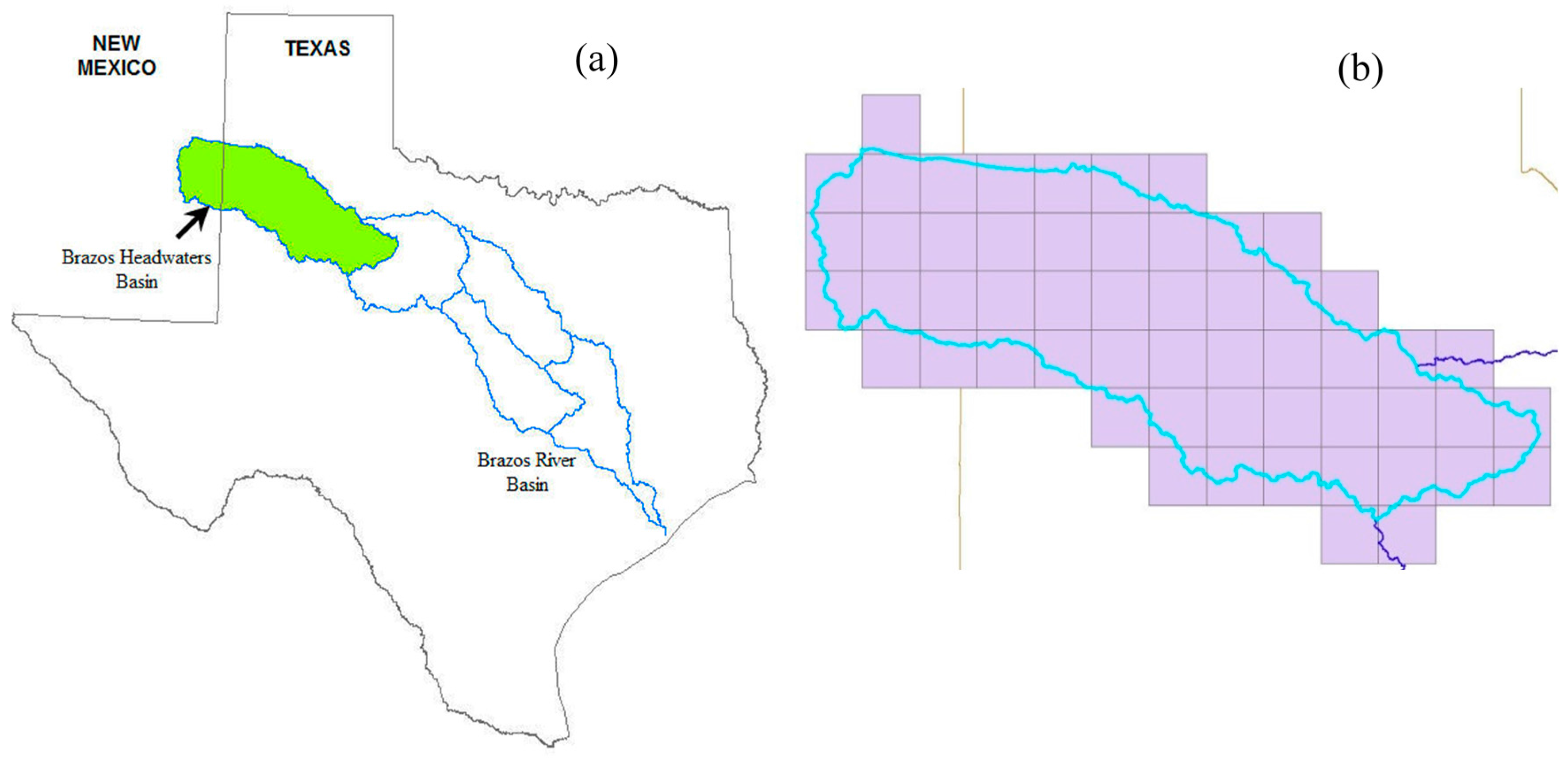
In this analysis, we considered three future periods: early 21st century 2011–2030 (2020s), mid-21st century 2046–2065 (2055s), and late 21st century 2080–2099 (2090s); and three greenhouse gas emissions scenarios (B1: low emissions scenario, A1B: moderate emissions scenario, and A2: high emissions scenario).

2.1. Study Site

The site used in this study was the Brazos Headwaters Basin (Hydrological Unit Code (HUC) = 120,500), the upper sub-basin of the Brazos River Basin, which is the second largest river basin within the state of Texas (Figure 1). It extends from northern west Texas to New Mexico, covering 37,558 km2. The major streams in this headwater basin are Salt Fork Brazos River and Double Mountain Fork Brazos River. These are small ephemeral streams, which relatively drain large amounts of land but do not produce much streamflow [34]. The major agricultural crops grown on this basin are wheat, sorghum, corn, and cotton.

2.2. Climate Data Input

Daily gridded precipitation, solar radiation, and minimum temperature (Tmin) and maximum temperature (Tmax) data from the National Centers for Environmental Prediction (NCEP) Climate Forecast System Reanalysis (CFSR) Global Weather Data for SWAT [35] for the 1981–2010 period were used as the historical daily climate data (hereafter referred as observed data). These observed data were used to calibrate the LARS-WG model (which is discussed in detail in Section 2.3) as part of the downscaling of monthly climate outputs from 15 GCMs for the study area (Figure 1). The observed (gridded) data are available at ~38 km resolution for the entire globe [36]. Several studies have successfully used these data for different studies, e.g., [37,38].

2.3. Downscaling of GCMs Outputs

Climate projections of 15 GCMs (Table 1) that were included in the Intergovernmental Panel on Climate Change (IPCC) 4th Assessment Report (AR4) on Climate Model Intercomparison Project (CMIP3) were downscaled for the study Basin using LARS-WG (version 5.0) stochastic model. It is worth noting that while the IPCC’s fifth assessment report (AR5) is the most recent on emissions scenarios, studies show that there were no significant improvements in accuracy of the GCMs in the IPCC-AR5. Knutti and Sedláček [39] reported that projected global temperature change from the new models was similar to the fourth assessment report (AR4) that was used in this study, and the spatial patterns of temperature and precipitation change were consistent with those of the AR4.
The LARS-WG model approximates probability distributions of dry and wet series, daily precipitation, Tmin and Tmax, and solar radiation using a semi-empirical distribution (SED), which is defined by the cumulative probability function (CDF) of a variable [40]. The semi-empirical distribution given by Emp = {a0, ai; hi, i = 1, …, 10} represents a histogram with 10 intervals [ai−1, ai], where ai−1 < ai and hi denotes the number of events from the observed data in the ith interval. SED uses 23 intervals to ensure more accurate representation of the observed distribution compared with the 10 used in the previous version [40]. Probability (pi) of a variable vi is calculated as:
Vi = min {v:P(vobs ≤ v) ≥ pi} i = 0, …, n,
where P() represents probability based on observed data {vobs}, p0 and pn are fixed parameters with corresponding values of 0 and 1, respectively. Details of LARS-WG can be found in Semenov and Stratonovitch [40].
Potential future climate scenarios were predicted for three periods (i.e., the 2020s, 2055s, and 2090s) under three different Greenhouse Gas (GHG) emissions scenarios (B1: low emissions scenario, A1B: moderate emissions scenario, and A2: high emissions scenario) using outputs from 15 GCMs available through LARS-WG model. LARS-WG model was calibrated using 30 years (1981–2010) of observed data. The calibration produced parameter files, which were later used to generate synthetic weather data with similar statistical properties of the observed data. Changes in weather parameters (precipitation and temperature) derived from GCMs were also used by LARS-WG to generate synthetic data under a particular climate change scenario for three future periods. To account for GCMs biases, the projections were statistically downscaled using the LARS-WG stochastic weather generator [33]. The observed data from 1981 to 2010 were used to characterize the current climate. LARS-WG produces synthetic time series data of daily temperature (Tmin and Tmax), precipitation, and solar radiation, based on the probability distributions of long-term observations.

2.4. Probability Distribution of Future Climates and Extreme Indices

The probability distributions of daily temperature (minimum and maximum) and precipitation were computed for future periods and the nonparametric Kolmogorov–Smirnov (K-S) statistical test was performed using the R software [41] to test the existence of significant differences between the probability distributions of climate parameters of future periods compared with the baseline period. Probability distributions for the four periods were determined by combining daily climatic data from 55 grids. Climate extreme indices provide key information for informed climate change mitigation and adaptation decisions [42]. Calculated frequency distributions of selected climate extremes for different future periods were used to investigate the intensity and frequency of climate extremes under projected climate change scenarios. Thus, frequency and intensity of climate extremes for selected temperature and precipitation extreme indices from a set of 27 core descriptive indices of climate extremes recommended by the joint CCl/WCRP-Clivar/JCOMM Expert Team on Climate Change Detection Monitoring and Indices [9] were assessed. Studied extreme indices include: Frost days (FD0), tropical nights (TR20), summer days (SU25), and ice days (ID0) that represent annual number of days with Tmin < 0 °C, Tmin > 20 °C, Tmax > 25 °C, Tmax < 0 °C, respectively; and RR1, RR5, RR10, and RR20 that represent number of days with prec ≥ 1, prec ≥ 5, prec ≥ 10, and prec ≥ 20 mm, respectively. Frequency distributions of the selected indices were computed in R [41] based on daily time series precipitation and temperature data generated using LARS-WG.

2.5. Meteorological Drought

The Standardized Precipitation Index (SPI) [10], a tool that is commonly used for monitoring drought by fitting probability distribution of historical rainfall observations [13,43], was used to assess drought frequency and intensities using observed and synthetic climate data for three periods (2020s, 2055s, and 2090s). In this study, we were interested in meteorological droughts and their impact on agriculture, thus we calculated three-month (short-term) drought frequencies under future potential climate change scenarios of the three future periods. Frequency distributions of different SPI indices under potential future climate scenarios were compared with the frequency distribution of the baseline (1981–2010). Since, SPI indices are normalized values, wetter and drier climates can be represented in the same way where positive SPI indices represent wet periods, while negative values indicate dry periods. While SPI is not a drought-forecasting tool, it can provide useful information on the nature of drought intensity and frequency as a result of climate change. While SPI is only based on precipitation records, unlike Standard Precipitation Evapotranspiration Index (SPEI), which is based on precipitation and evapotranspiration, it can be effectively used for monitoring meteorological droughts in the USA [43]. Projected changes in drought indices can also indicate the effect of climate change on climate extremes. In this study, we classified drought intensities following the approach used by the United States Drought Monitor (Table 2), where drought category D1 represents the least intense drought, while D4 is the most intense drought. Drought indices were computed using the SPEI package in R [41].

3. Results and Discussion

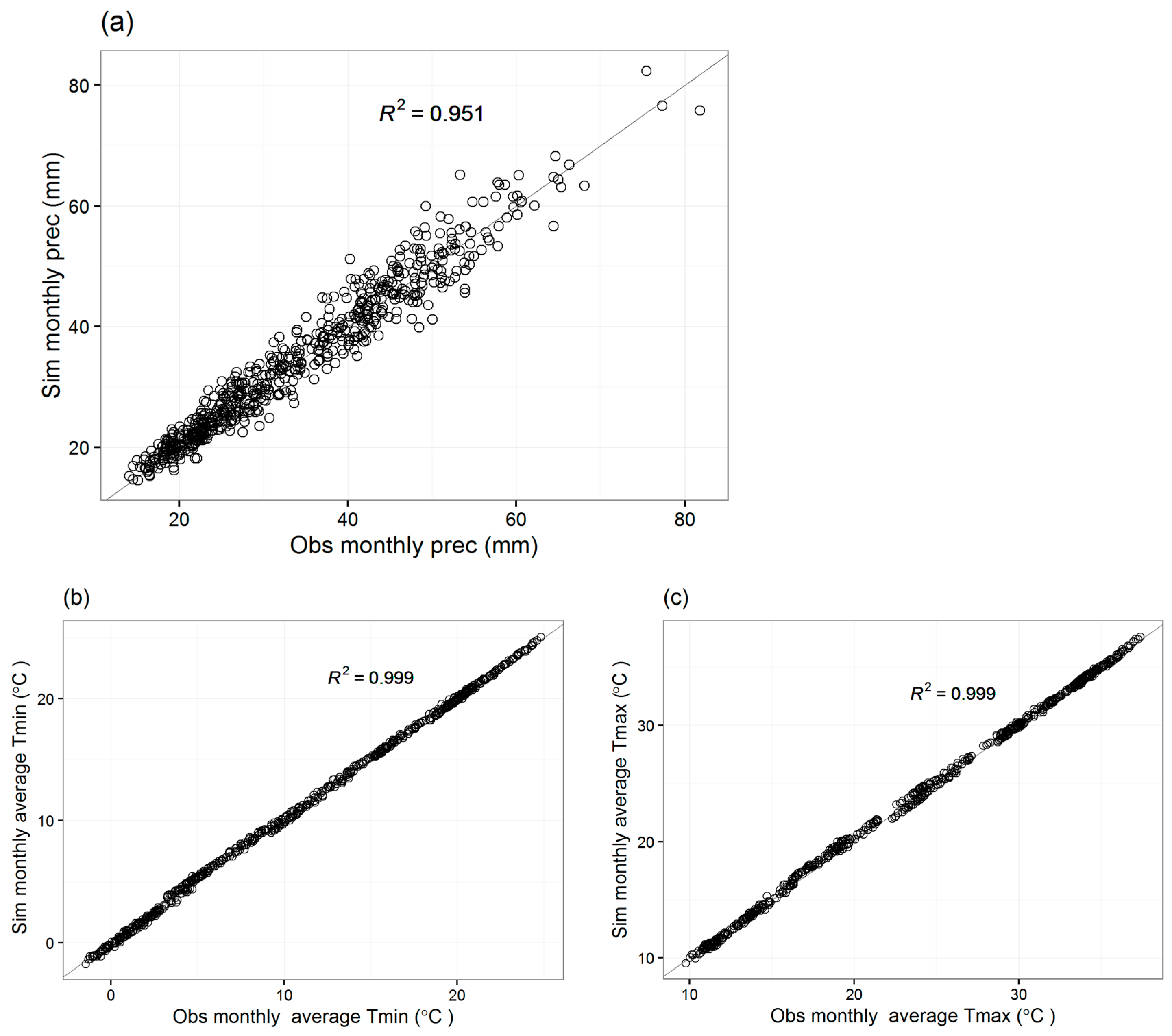
3.1. Performance of the LARS-WG Model

Observed and simulated mean monthly total precipitation, Tmin and Tmax, at the 55 grids of the study basin are shown in Figure 2. Results indicate that the model predicts Tmin and Tmax very well, whereas the performance of the model in predicting monthly precipitation was acceptable. Similarly, model validation results (for one grid at the center of the basin) indicate a satisfactory performance of the model in simulating daily Tmin and Tmax, while its performance was less effective in simulating daily precipitation. The model under- and overpredicts precipitation (Figure 2a). The findings of this work were in partial agreement with Agarwal et al. [6], who also reported that LARS-WG underpredicted precipitation. In general, the current results are in agreement with other studies that reported lower performance of LARS-WG in predicting precipitation compared with its simulation of air temperature (Tmin and Tmax) [7,30]. It is also worth noting that other downscaling models (e.g., SDSM) exhibited lower performance in predicting precipitation compared with temperature [7,19]. Therefore, based on the overall performance of LARS-WG, especially its prediction of monthly climatic variables (Tmin and Tmax), we conclude that the model can be used to effectively predict climatic variables for different purposes including climate change impact studies.

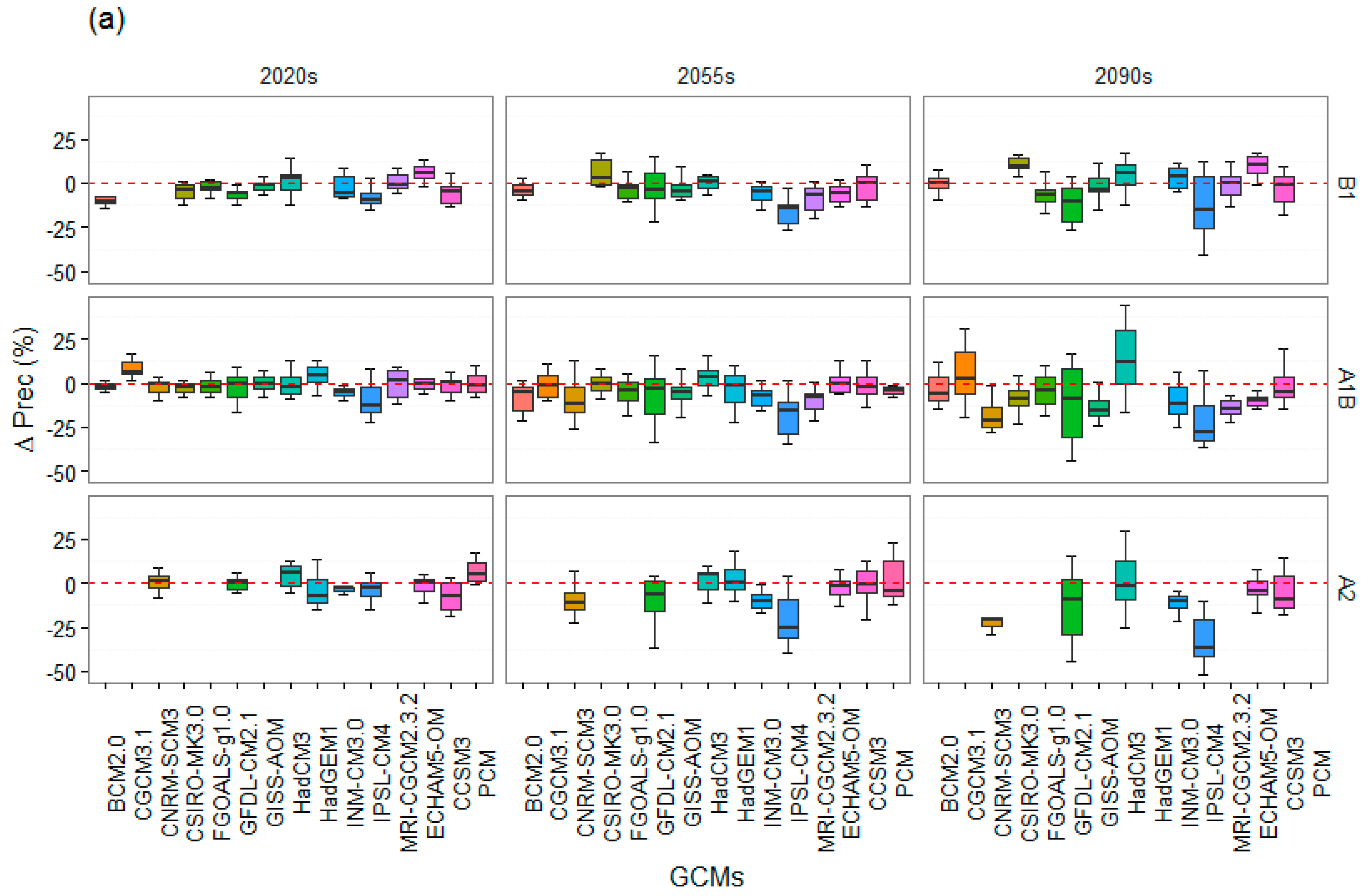
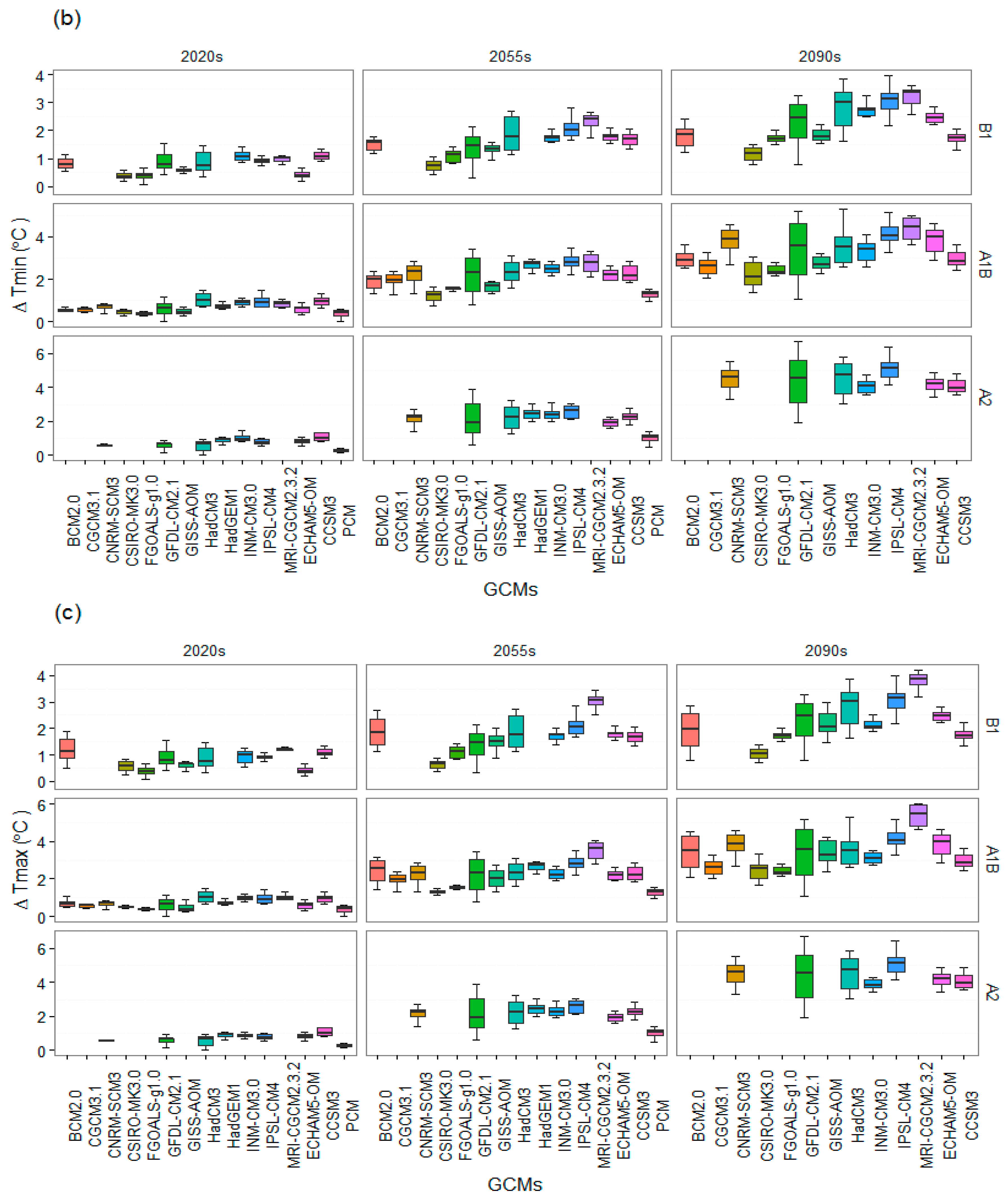
3.2. Future Climate Projections and Uncertainties of GCMs

Annual precipitation is projected to decrease on average by 1.8%, 5.2%, and 6.8% in the 2020s, 2055s, and 2090s (Table 3), respectively. Most of the GCMs predicted that precipitation will decrease during all three future periods, but a greater reduction is predicted in the 2055s and 2090s (Figure 3). Particularly, a significant reduction (12.3%) of annual precipitation is predicted in the 2090s under the A2 (high) emissions scenario. On the other hand, both Tmin and Tmax are projected to increase by (0.7, 2.0, and 3.3 °C) and (0.7, 2.0, and 3.4 °C) in the 2020s, 2055s, and 2090s, respectively, compared with the baseline (1981–2010) (Table 3). Overall, there was no substantial difference between the emissions scenarios during the 2020s; however, significantly higher temperatures are projected under A1B (moderate) and A2 (high) emissions scenarios during the 2055s and 2090s. The findings of the current study are in agreement with those of Schoof [2], who reported a projected decline in annual total precipitation in the Southwest USA. Similarly, Singh et al. [45] reported negative anomalies of total annual precipitation in the Southwestern USA. However, positive increases in precipitation were reported in areas with monsoon climates, such as Nepal [6]. Schoof [2] also reported positive increases in annual precipitation in the Northeast, Pacific Northwest, and the high elevations of the Rocky Mountains.
Projections based on the 15 GCMs show consistent decreases in precipitation under all emissions scenarios for all future periods. However, there was a significant inconsistency of GCMs between emissions scenarios in predicting precipitation (Figure 3). There was no agreement between GCMs in predicting future precipitation; some GCMs (e.g., GFDL-CM2.1) showed significant prediction uncertainty, with prediction ranges between +15% and −45% in the 2090s under A1B (moderate) and A2 (high) emissions scenarios (Figure 3a). While all GCMs predicted increases in Tmin and Tmax under all emissions scenarios and periods, GCMs uncertainty is also present in Tmin and Tmax prediction (Figure 3b,c). Overall, the variability between GCMs increased substantially for the 2090s. Differences between GCMs in predicting climate variables indicate underlying uncertainties associated with all these models. Agarwal et al. [6] reported that GCMs show disagreements in predicting changes in precipitation. Semenov and Stratonovitch [40] indicated that these uncertainties are due to variations in initial conditions or model parameterizations.

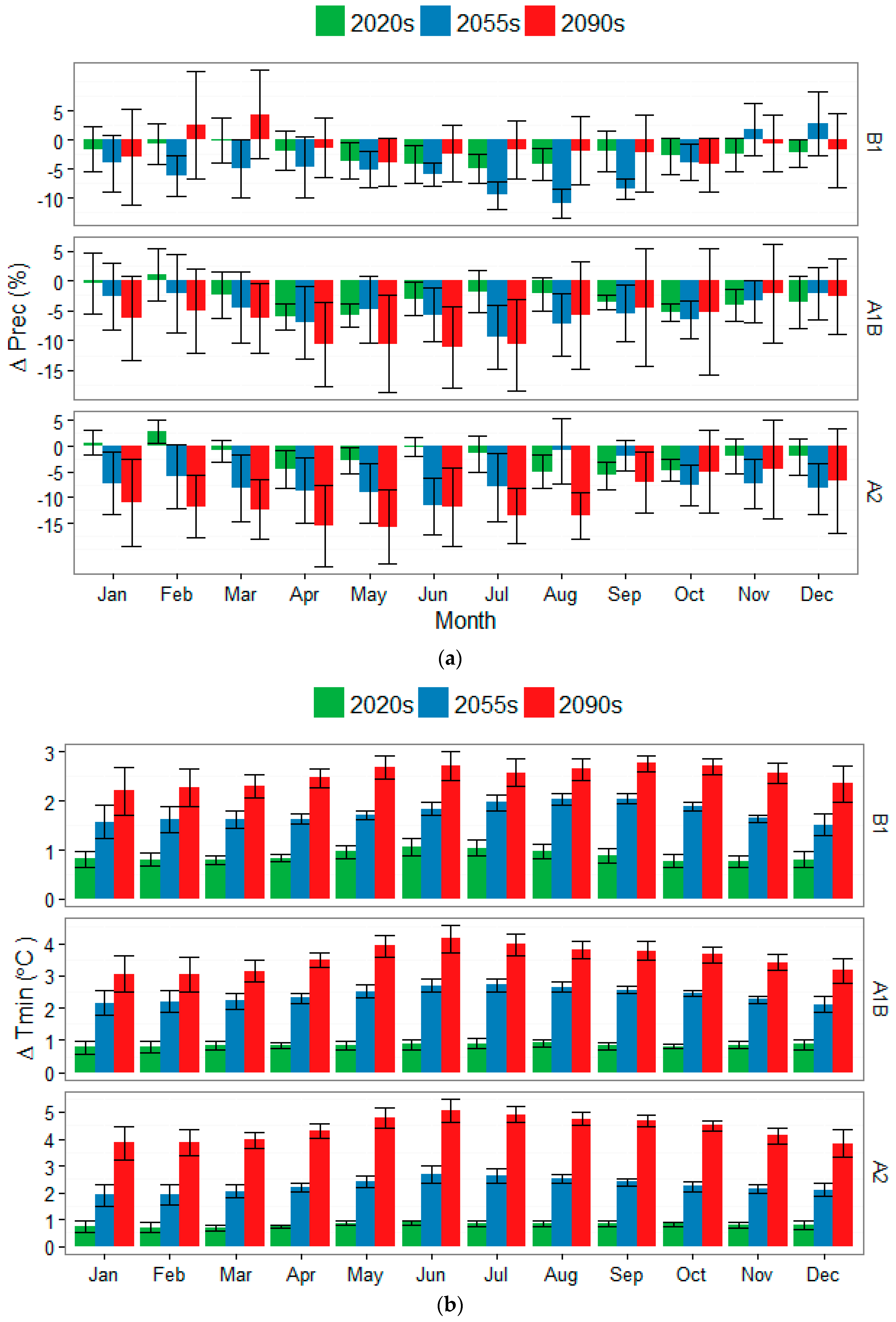
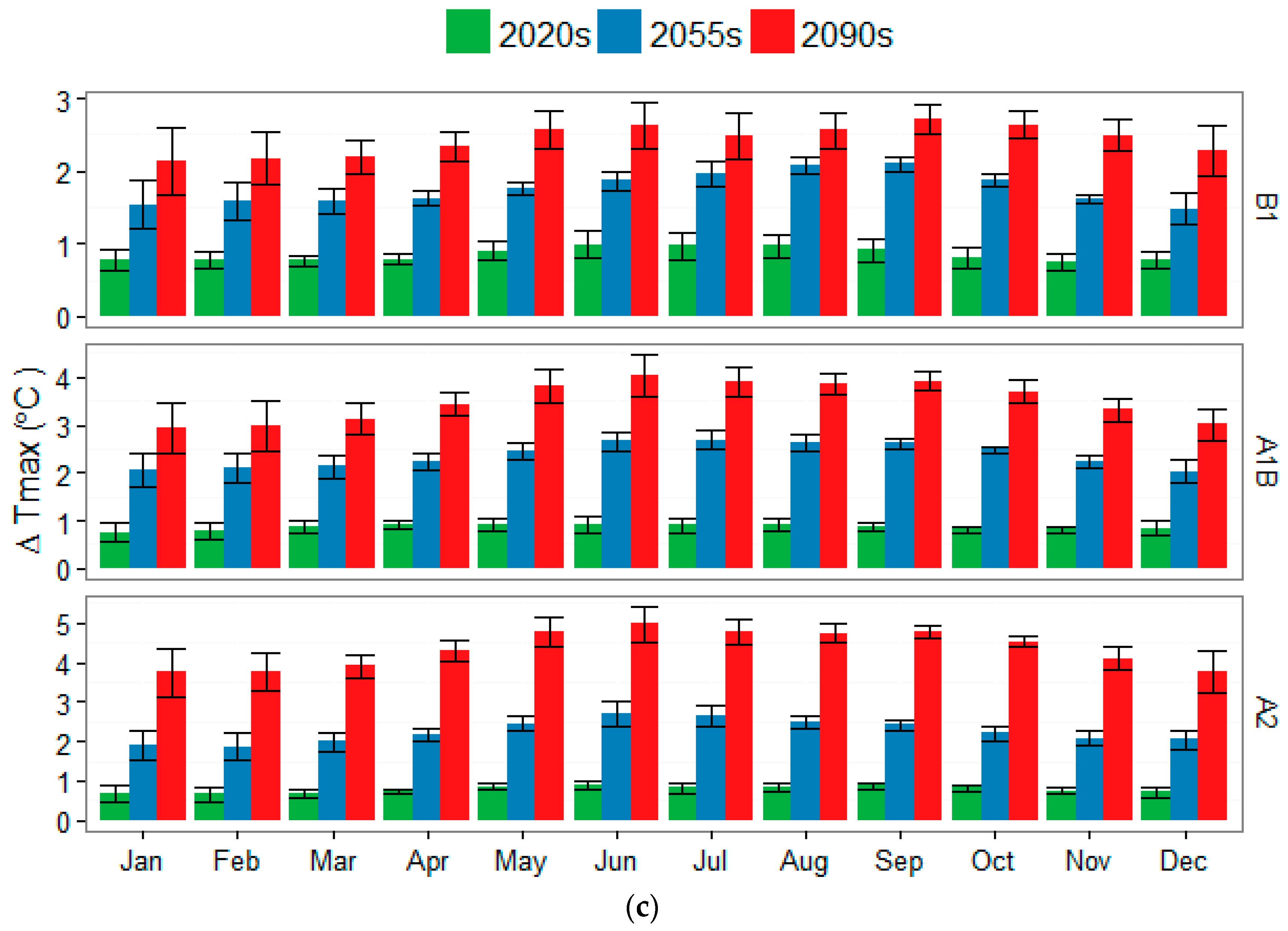
3.3. Seasonal Changes of Projected Climate

Monthly precipitation is projected to experience a substantial reduction throughout most of the year (Figure 4a). However, precipitation is expected to increase during the winter months (January–March) in the 2020s and February and March in the 2090s under the A1B (moderate) and A2 (high), and B1 (low) emissions scenarios, respectively. Projections for the 2055s show a consistent decrease under all emissions scenarios. Consistently, significant reductions in monthly precipitation are projected during the 2090s. Projected decreases in precipitation concur with projections by Schoof [2], who reported moderate precipitation decreases for the Southern USA based on the fifth assessment report (AR5) [16]. Similarly, Singh et al. [45] projected strong dry trends in seasonal precipitation for the Southwest USA. Moreover, average temperature (Tmin and Tmax) projections show consistent increases during all three periods; twofold increases in Tmin and Tmax are projected in the 2090s compared with projected increases in the 2020s and 2055s (Figure 4b,c). There was no substantial difference between projections of monthly precipitation under emissions scenarios A1B (moderate) and A2 (high) during the 2020s and 2055s. However, a significantly greater reduction of precipitation is projected for the 2090s under the A2 (high) emissions scenario.

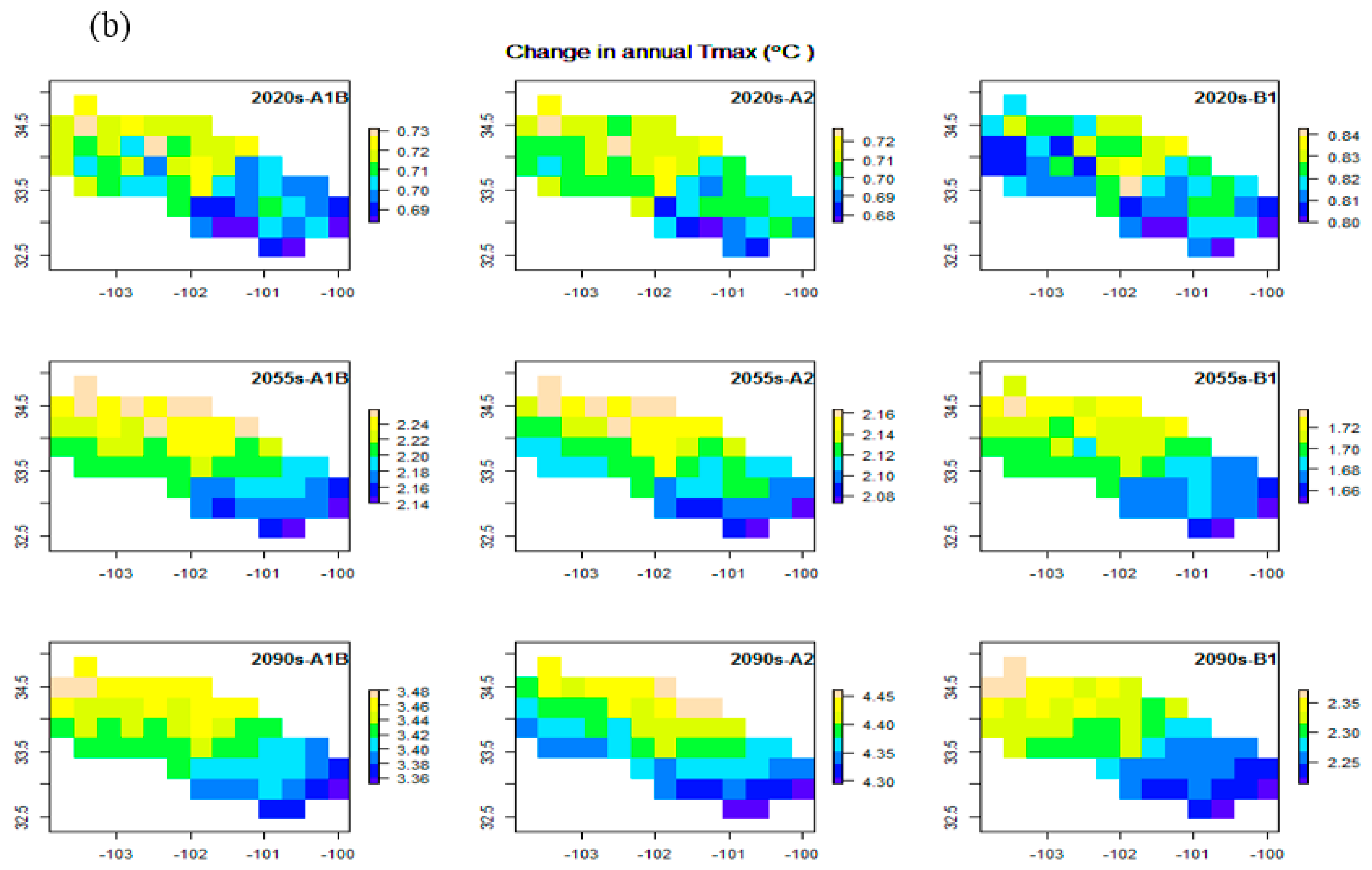
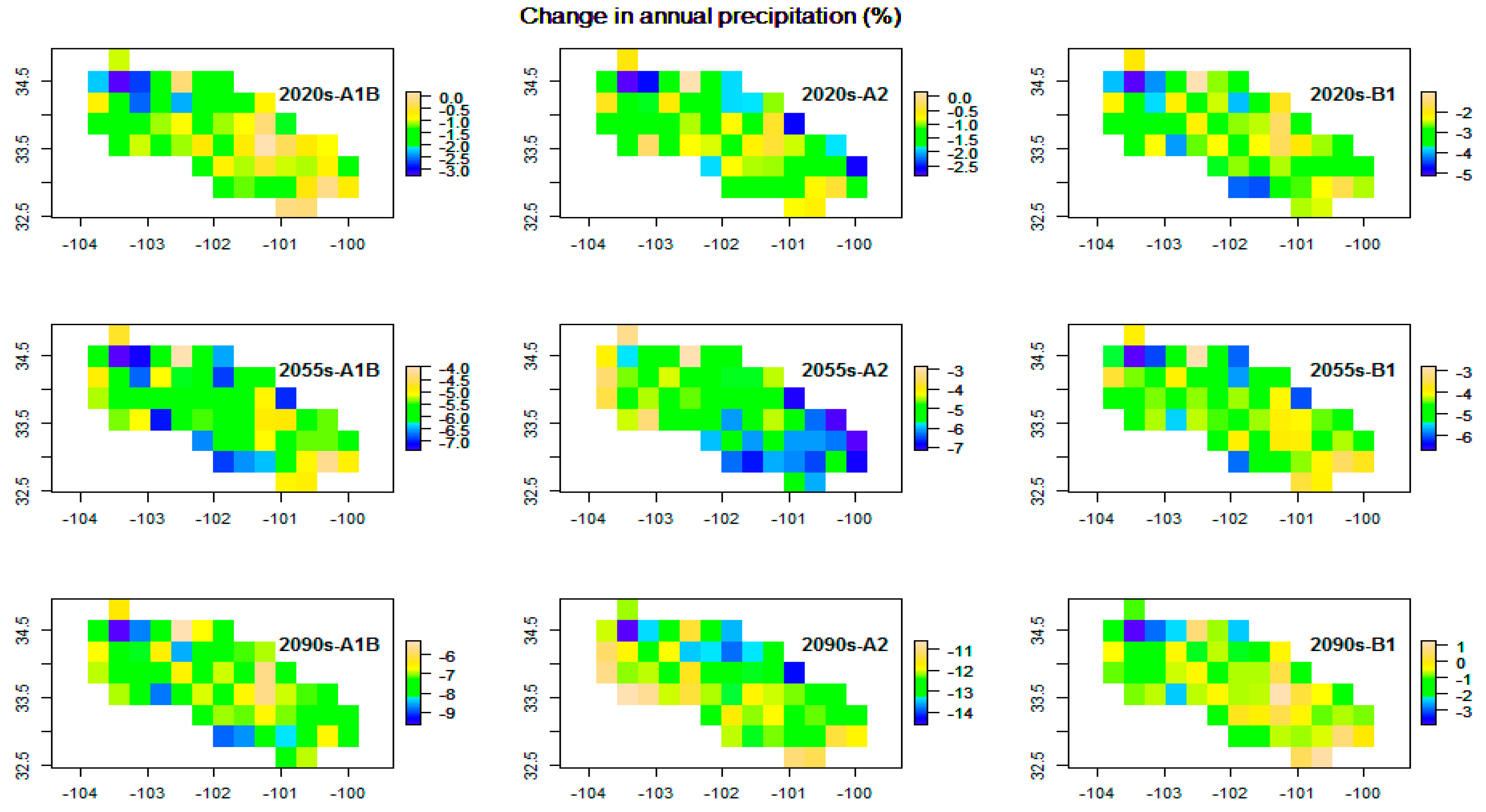
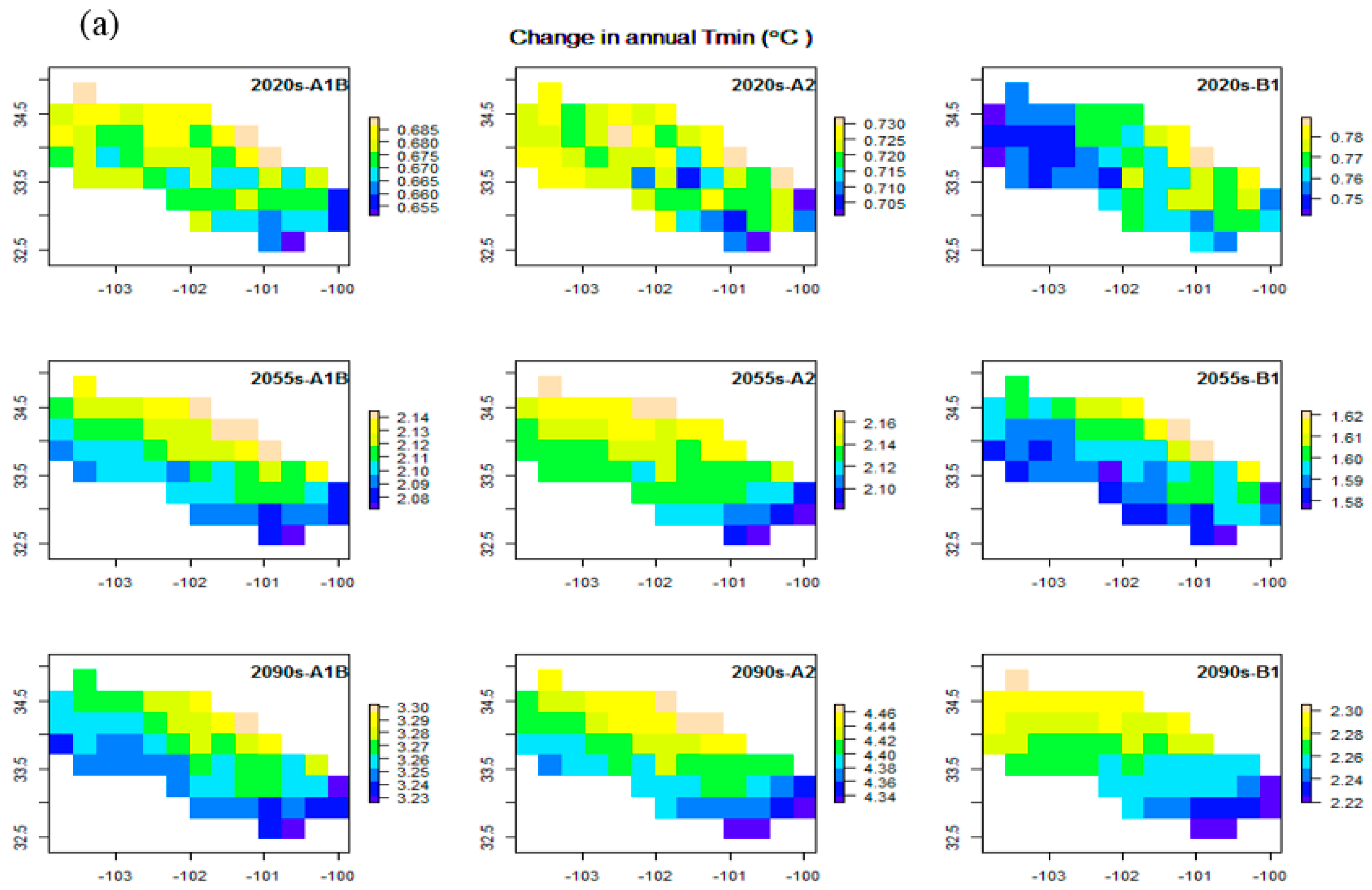
3.4. Spatial Changes in Projected Climates

Annual precipitation is projected to decrease across all grids in the Brazos Headwaters Basin under all emissions scenarios and for all three future periods; however, the maximum decrease in annual precipitation is predicted for the A2 (high) followed by A1B (moderate) emissions scenarios during the 2090s (Figure 5). The projected decrease in precipitation under the B1 (low) emissions scenario was slightly greater in the 2020s and on a par with the 2055s under the A1B (moderate) and A2 (high) emissions scenarios; however, the projected decrease under B1 was significantly smaller in the 2090s compared to that for the other two scenarios (Figure 5). Overall, the northwestern and southern parts of the Brazos Headwaters Basin are projected to experience a slightly greater decrease in precipitation under most emissions scenarios and all future periods (Figure 5). However, there was an exception, where a consistently greater decrease is projected under the A2 (high) emissions scenario in the 2055s for the southeastern part compared with the northwestern part of the basin (Figure 5).
On the other hand, annual average Tmin and Tmax are projected to increase under all emissions scenarios and all three future periods (Figure 6). The greatest increases in both Tmin and Tmax are projected in the 2090s under the A2 (high) emissions scenario, followed by A1B (moderate emissions scenario). Generally, projected increases of Tmin and Tmax will be in the upper range in the southern and southeastern part of the basin (Figure 6). Compatible with annual precipitation projections under the B1 (low) emissions scenario, projected increases of Tmin and Tmax are slightly greater under the B1 (low) emissions scenario in the 2020s, while projected increases under the same scenario are significantly lower in the 2055s and 2090s compared to the other two scenarios (Figure 6).

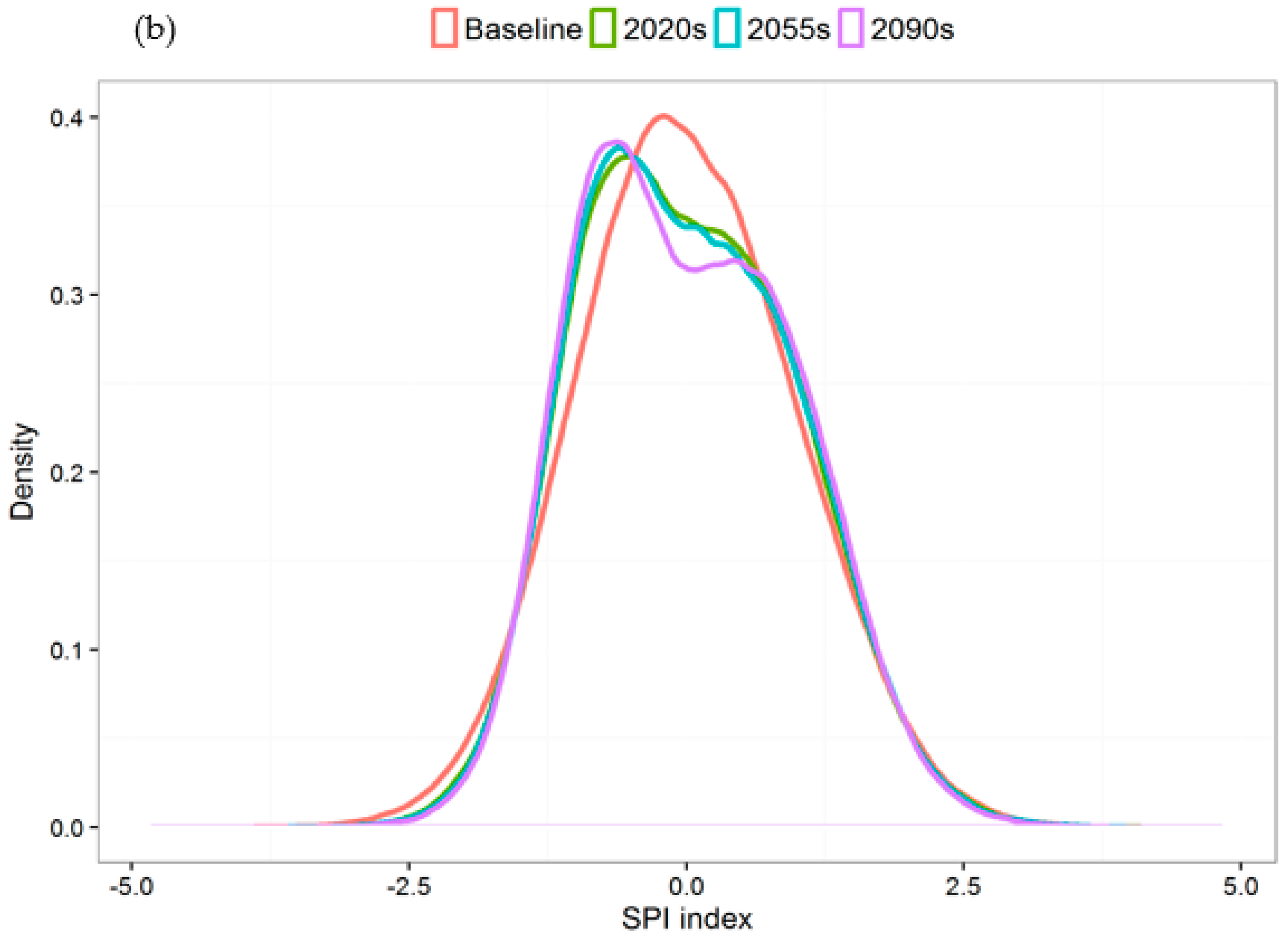
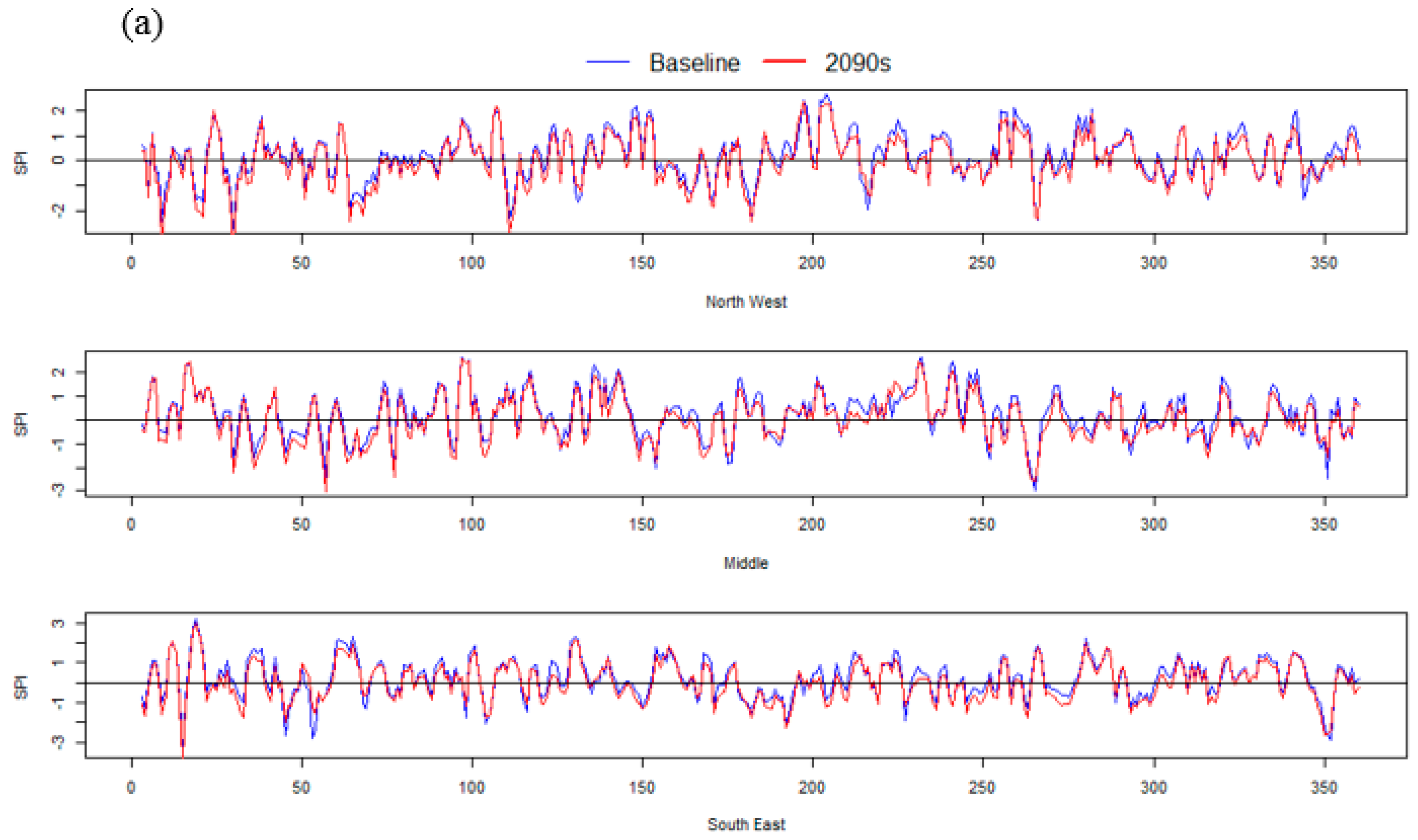
3.5. Meteorological Drought Indices

Time series meteorological (three-month) drought indices, which would provide insights about possible agricultural droughts, calculated based on monthly rainfall data from the baseline and the 2090s periods, are presented for three selected grids (South East, Middle, and North West parts of the Brazos Headwaters Basin) (Figure 7a). According to McKee et al. [10], drought occurs when SPI is continuously negative and reaches ≤−1; however, positive SPI indicates the end of a drought event. While the results show slight shifts in the probability distribution of drought indices for future periods compared to the baseline, the predicted shifts are not statistically significant (Figure 7b). Ford and Labosier [46] reported that infrequent drought persistence in the Southeast United States makes seasonal drought forecasting difficult.
However, frequency analysis of meteorological drought indices for each drought category (see Table 2) showed that there was no considerable change in frequency distribution of drought indices (data not shown). However, while our results did not indicate significant changes in the intensity of droughts, it is expected that droughts of the same intensity as the historic period would occur in future periods (data not shown).

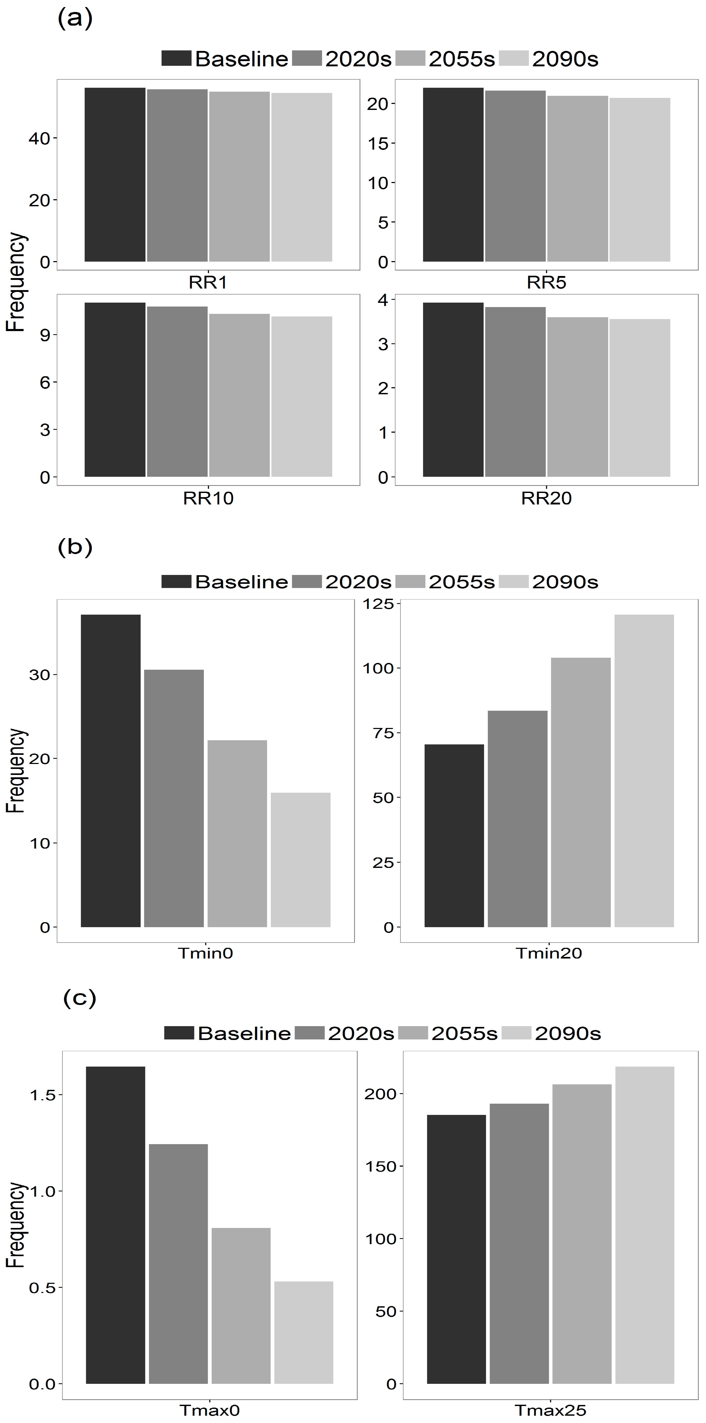
3.6. Extreme Climate Indices

Overall, frequency of precipitation and temperature indices show relatively considerable changes (Figure 8). The frequency analysis of rainfall indices, except RR1, is predicted to decrease as we progress toward the end of the 21st century. This indicates significant decreases in the number of wet days (RR5) and heavy precipitation days (RR10 and RR20) (Figure 8a). Temperature indices of frost days and ice days are projected to decrease, while tropical nights and summer days are expected to increase (Figure 8b,c). Increases in tropical nights (Tmin > 20 °C) and summer days (Tmax > 25 °C) will be greater by orders of magnitude compared with the projected decreases in the number of frost days (Tmin < 0 °C) and ice days (Tmax < 0 °C). Our results of RR5 indices concur with those reported by Arriaga-Ramírez and Cavazos [47], who found similar results for the state of Texas. However, Mishra and Singh [48] reported mixed results of extreme precipitation occurrence in Texas. On the other hand, our projections of decreases in heavy precipitation contradict those reported by Mullens et al. [49] and Arriaga-Ramírez and Cavazos [47], who projected increases in the frequency and intensity of precipitation for the state of Texas. Our projections regarding temperature indices concur with the findings of Mutiibwa et al. [50], who reported an overall increase in warming trends temperature indices in the United States. Moreover, Kolmogorov–Smirnov (K-S) statistical test results show that the probability distributions of minimum and maximum temperature and precipitation for future periods are significantly different from the probability distributions of the baseline (Figure 9).

4. Conclusions

This study assessed potential future climates and climate extremes, and evaluated spatial and temporal changes in prec., Tmax, and Tmin for the Brazos Headwaters Basin under three greenhouse gas emissions scenarios (A2, A1B, and B1) for three future periods (2020s, 2055s, and 2090s). In addition, the frequency and intensity of meteorological droughts, and extreme climate (precipitation and temperature) indices defined by ETCCMDI, were also analyzed. The LARS-WG model was used to downscale precipitation and temperature projections from 15 GCMs. Daily gridded climate data obtained from CFSR were used for calibration and validation of the LARS-WG model. The LARS-WG model predicted monthly average Tmin and Tmax very well, whereas its performance in predicting monthly precipitation was only acceptable. Results show that precipitation is projected to decrease on average by 1.8%, 5.2%, and 6.8% in the 2020s, 2055s, and 2090s, respectively. While average ensemble projections from 15 GCMs consistently show decreases in precipitation under all emissions scenarios for all future periods, significant inconsistency and variations were observed between GCMs in predicting precipitation. Individual GCMS projections of monthly precipitation changes compared with the baseline varied between −9.6% to +7.89%, −18.4% to +3.51%, and −29.8% to +14.91% during the 2020s, 2055s, and 2090s, respectively. On the other hand, however, all GCMs consistently predicted increases in Tmin by 0.7, 2.0, and 3.3 °C; and Tmax by 0.7, 2.0, and 3.4 °C in the 2020s, 2055s, and 2090s, respectively.
While annual precipitation is projected to decrease across all grids in the Brazos Headwaters Basin under all emissions scenarios and future periods, the northwestern and southern parts of the basin are mostly projected to experience a slightly greater decrease in precipitation compared with other parts of the basin. Moreover, precipitation indices show slight decreases in the number of wet and heavy precipitation days for all future periods. On the other hand, temperature indices show that frost and ice days are projected to decrease, while tropical nights and summer days are expected to increase. Results based on precipitation and temperature indices suggest that dry spells will be longer and more intense in future periods. However, there were no significant changes between the baseline and projected drought frequency and severity for future periods.
Overall, while this study provides insights on how future climate and climate extremes would unfold in the Brazos headwaters basin, additional work is needed to quantify how these projected changes in precipitation and temperature will affect water resources allocations for different users (e.g., agriculture, domestic, industries, and ecosystems).

Acknowledgments

This work was supported by the USDA National Institute of Food and Agriculture, Evans-Allen project and Texas A&M AgriLife Research.

Author Contributions

Ripendra Awal, Haimanote K. Bayabil, and Ali Fares contributed significantly in formulating the research questions, downscaling Global Circulation Model outputs, data analysis, and write-up of the manuscript. They also contributed in addressing reviewers comments during the review process and proof reading of the accepted manuscript.

Conflicts of Interest

The authors declare no conflict of interest.

References

  1. O’sullivan, T.M. Environmental Security is Homeland Security: Climate Disruption as the Ultimate Disaster Risk Multiplier. Risk Hazards Crisis Public Policy 2015, 6, 183–222. [Google Scholar] [CrossRef]
  2. Schoof, J.T. High-Resolution Projections of 21st Century Daily Precipitation for the Contiguous U.S. J. Geophys. Res. Atmos. 2015, 120, 3029–3042. [Google Scholar] [CrossRef]
  3. Thornton, P.K.; Ericksen, P.J.; Herrero, M.; Challinor, A.J. Climate variability and vulnerability to climate change: A review. Glob. Chang. Biol. 2014, 20, 3313–3328. [Google Scholar] [CrossRef] [PubMed]
  4. Haines, A.; Kovats, R.S.; Campbell-Lendrum, D.; Corvalan, C. Climate Change and Human Health: Impacts, Vulnerability and Public Health. Public Health 2006, 120, 585–596. [Google Scholar] [CrossRef] [PubMed]
  5. Mcgeehin, M.A.; Mirabelli, M. The Potential Impacts of Climate Variability and Change on Temperature-Related Morbidity and Mortality in the United States. Environ. Health Perspect. 2001, 109, 185–189. [Google Scholar] [CrossRef] [PubMed]
  6. Agarwal, A.; Babel, M.S.; Maskey, S. Analysis of Future Precipitation in the Koshi River Basin, Nepal. J. Hydrol. 2014, 513, 422–434. [Google Scholar] [CrossRef]
  7. Hassan, Z.; Shamsudin, S.; Harun, S. Application of SDSM and LARS-WG For Simulating and Downscaling of Rainfall and Temperature. Theor. Appl. Climatol. 2014, 116, 243–257. [Google Scholar] [CrossRef]
  8. Easterling, D.R.; Meehl, G.A.; Parmesan, C.; Changnon, S.A.; Karl, T.R.; Mearns, L.O. Climate extremes: Observations, modeling, and impacts. Science 2000, 289, 2068–2074. [Google Scholar] [CrossRef] [PubMed]
  9. Klein Tank, A.M.G.; Zwiers, F.W.; Zhang, X. Guidelines on Analysis of Extremes in a Changing Climate in Support of Informed Decisions For Adaptation, Climate Data and Monitoring; WMO-TD No. 1500; World Meteorological Organization (WMO): Geneva, Switzerland, 2009. [Google Scholar]
  10. Mckee, T.B.; Doesken, N.J.; Kleist, J. Others the Relationship of Drought Frequency and Duration to Time Scales. In Proceedings of the 8th Conference on Applied Climatology, Anaheim, CA, USA, 17–22 January 1993; American Meteorological Society: Boston, MA, USA, 1993; Volume 17, pp. 179–183. [Google Scholar]
  11. Moorhead, J.E.; Gowda, P.H.; Singh, V.P.; Porter, D.O.; Marek, T.H.; Howell, T.A.; Stewart, B.A. Identifying and evaluating a suitable index for agricultural drought monitoring in the Texas high plains. JAWRA J. Am. Water Resour. Assoc. 2015, 51, 807–820. [Google Scholar] [CrossRef]
  12. Van Loon, A.F. Hydrological drought explained: Hydrological drought explained. Wiley Interdiscip. Rev. Water 2015, 2, 359–392. [Google Scholar] [CrossRef]
  13. Edwards, D.C.; Mckee, T.B. Characteristics of 20th Century Drought in the United States at Multiple Time Scales; Atmospheric Science, Colorado State University: Fort Collins, CO, USA, 1997. [Google Scholar]
  14. Busuioc, A.; Von Storch, H.; Schnur, R. Verification of GCM-Generated regional seasonal precipitation for current climate and of statistical downscaling estimates under changing climate conditions. J. Clim. 1999, 12, 258–272. [Google Scholar] [CrossRef]
  15. Randall, D.A.; Wood, R.A.; Bony, S.; Colman, R.; Fichefet, T.; Fyfe, J.; Kattsov, V.; Pitman, A.; Shukla, J.; Srinivasan, J. Others climate models and their evaluation. In Climate Change 2007: The Physical Science Basis. Contribution of Working Group I to the Fourth Assessment Report of the IPCC (Far); Cambridge University Press: Cambridge, UK, 2007; pp. 589–662. [Google Scholar]
  16. Stocker, T.F.; Qin, D.; Plattner, G.K.; Tignor, M.; Allen, S.K.; Boschung, J.; Nauels, A.; Xia, Y.; Bex, B.; Midgley, B.M. IPCC, 2013: Climate Change: The Physical Science Basis. Contribution of Working Group I to the Fifth Assessment Report of the Intergovernmental Panel on Climate Change; Cambridge University Press: Cambridge, UK, 2013. [Google Scholar]
  17. Wilby, R.L.; Wigley, T.M.L.; Conway, D.; Jones, P.D.; Hewitson, B.C.; Main, J.; Wilks, D.S. Statistical downscaling of general circulation model output: A comparison of methods. Water Resour. Res. 1998, 34, 2995–3008. [Google Scholar] [CrossRef]
  18. Wilby, R.L.; Dawson, C.W. The statistical downscaling model: Insights from one decade of application. Int. J. Climatol. 2013, 33, 1707–1719. [Google Scholar] [CrossRef]
  19. Wilby, R.L.; Yu, D. Rainfall and temperature estimation for a data sparse region. Hydrol. Earth Syst. Sci. 2013, 17, 3937–3955. [Google Scholar] [CrossRef]
  20. Casanueva, A.; Herrera, S.; Fernández, J.; Gutiérrez, J.M. Towards a fair comparison of statistical and dynamical downscaling in the framework of the EURO-CORDEX initiative. Clim. Chang. 2016, 137, 411–426. [Google Scholar] [CrossRef]
  21. Boé, J.; Terray, L.; Habets, F.; Martin, E. Statistical and dynamical downscaling of the seine basin climate for hydro-meteorological studies. Int. J. Climatol. 2007, 27, 1643–1655. [Google Scholar] [CrossRef]
  22. Gutmann, E.D.; Rasmussen, R.M.; Liu, C.; Ikeda, K.; Gochis, D.J.; Clark, M.P.; Dudhia, J.; Thompson, G.A. Comparison of statistical and dynamical downscaling of winter precipitation over complex terrain. J. Clim. 2012, 25, 262–281. [Google Scholar] [CrossRef]
  23. Nover, D.M.; Witt, J.W.; Butcher, J.B.; Johnson, T.E.; Weaver, C.P. The effects of downscaling method on the variability of simulated watershed response to climate change in five us basins. Earth Interact. 2016, 20, 1–27. [Google Scholar] [CrossRef]
  24. Wilby, R.L.; Wigley, T.M.L. Downscaling general circulation model output: A review of methods and limitations. Prog. Phys. Geogr. 1997, 21, 530–548. [Google Scholar] [CrossRef]
  25. Hewitson, B.C.; Crane, R.G. Climate downscaling: Techniques and application. Clim. Res. 1996, 7, 85–95. [Google Scholar] [CrossRef]
  26. Schmidli, J.; Goodess, C.M.; Frei, C.; Haylock, M.R.; Hundecha, Y.; Ribalaygua, J.; Schmith, T. Statistical and dynamical downscaling of precipitation: An evaluation and comparison of scenarios for the european alps. J. Geophys. Res. 2007, 112, 1–20. [Google Scholar] [CrossRef]
  27. Dixon, K.W.; Lanzante, J.R.; Nath, M.J.; Hayhoe, K.; Stoner, A.; Radhakrishnan, A.; Balaji, V.; Gaitán, C.F. Evaluating the stationarity assumption in statistically downscaled climate projections: Is past performance an indicator of future results? Clim. Chang. 2016, 135, 395–408. [Google Scholar] [CrossRef]
  28. Agarwal, A.; Babel, M.S.; Maskey, S.; Shrestha, S.; Kawasaki, A.; Tripathi, N.K. Analysis of temperature projections in the Koshi River Basin, Nepal. Int. J. Climatol. 2016, 36, 266–279. [Google Scholar] [CrossRef]
  29. Calanca, P.; Semenov, M.A. Local-Scale climate scenarios for impact studies and risk assessments: Integration of early 21st century ensembles projections into the ELPIS database. Theor. Appl. Climatol. 2013, 113, 445–455. [Google Scholar] [CrossRef]
  30. Chen, H.; Guo, J.; Zhang, Z.; Xu, C.-Y. Prediction of temperature and precipitation in Sudan and south Sudan by using LARS-WG in future. Theor. Appl. Climatol. 2013, 113, 363–375. [Google Scholar] [CrossRef]
  31. Semenov, M. Simulation of extreme weather events by a stochastic weather generator. Clim. Res. 2008, 35, 203–212. [Google Scholar] [CrossRef]
  32. Semenov, M.A. Development of high-resolution UKCIP02-Based climate change scenarios in the UK. Agric. For. Meteorol. 2007, 144, 127–138. [Google Scholar] [CrossRef]
  33. Semenov, M.A.; Barrow, E.M. LARS-WG: A Stochastic Weather Generator for Use in Climate Impact Studies, 3rd ed.; User Manual; Available online: http://www.rothamsted.ac.uk/sites/default/files/groups/mas-models/download/LARS-WG-Manual.pdf (accessed on 1 August 2014).
  34. Baldys, S.; Schalla, F.E. Base Flow (1966–2009) and Streamflow Gain and Loss (2010) of the Brazos River from the New Mexico-Texas State Line to Waco, Texas; U.S. Geological Survey, Scientific Investigations Report 2011-5224; U.S. Department of the Interior: Reston, VA, USA, 2016. Available online: http://dx.doi.org/10.3133/sir20115224 (accessed on 5 July 2016).
  35. Global Weather Data for SWAT. Available online: http://globalweather.tamu.edu/ (accessed on 1 December 2014).
  36. Saha, S.; Moorthi, S.; Pan, H.L.; Wu, X.; Wang, J.; Nadiga, S.; Tripp, P.; Kistler, R.; Woollen, J.; Behringer, D.; et al. The NCEP climate forecast system reanalysis. Bull. Am. Meteorol. Soc. 2010, 91, 1015–1057. [Google Scholar] [CrossRef]
  37. Dile, Y.T.; Srinivasan, R. Evaluation of CFSR climate data for hydrologic prediction in data-scarce watersheds: An Application in the Blue Nile River basin. JAWRA J. Am. Water Resour. Assoc. 2014, 50, 1226–1241. [Google Scholar] [CrossRef]
  38. Fuka, D.R.; Walter, M.T.; Macalister, C.; Degaetano, A.T.; Steenhuis, T.S.; Easton, Z.M. Using the climate forecast system reanalysis as weather input data for watershed models: Using CFSR as weather input data for watershed models. Hydrol. Process. 2014, 28, 5613–5623. [Google Scholar] [CrossRef]
  39. Knutti, R.; Sedláček, J. Robustness and uncertainties in the new CMIP5 climate model projections. Nat. Clim. Chang. 2012, 3, 369–373. [Google Scholar] [CrossRef]
  40. Semenov, M.; Stratonovitch, P. Use of multi-model ensembles from global climate models for assessment of climate change impacts. Clim. Res. 2010, 41, 1–14. [Google Scholar] [CrossRef]
  41. R Core Team. R: A Language and Environment for Statistical Computing; R Foundation for Statistical Computing: Vienna, Austria, 2016; Available online: https://www.r-project.org/ (accessed on 5 May 2016).
  42. Sillmann, J.; Kharin, V.V.; Zwiers, F.W.; Zhang, X.; Bronaugh, D. Climate extremes indices in the CMIP5 multimodel ensemble: Part 2. Future climate projections: CMIP5 projections of extremes indices. J. Geophys. Res. Atmos. 2013, 118, 2473–2493. [Google Scholar] [CrossRef]
  43. Quiring, S.M. Monitoring drought: An evaluation of meteorological drought indices. Geogr. Compass 2009, 3, 64–88. [Google Scholar] [CrossRef]
  44. United States Drought Monitor: U.S. Drought Monitor Classification Scheme. Available online: http://droughtmonitor.unl.edu/aboutus/classificationscheme.aspx (accessed on 15 May 2016).
  45. Singh, D.; Tsiang, M.; Rajaratnam, B.; Diffenbaugh, N.S. Precipitation extremes over the continental united states in a transient, high-resolution, ensemble climate model experiment: U.S. precipitation extremes with warming. J. Geophys. Res. Atmos. 2013, 118, 7063–7086. [Google Scholar] [CrossRef]
  46. Ford, T.; Labosier, C.F. Spatial patterns of drought persistence in the southeastern United States: Drought persistence in the southeast. Int. J. Climatol. 2014, 34, 2229–2240. [Google Scholar] [CrossRef]
  47. Arriaga-Ramírez, S.; Cavazos, T. Regional trends of daily precipitation indices in Northwest Mexico and Southwest United States. J. Geophys. Res. 2010, 115, 1–10. [Google Scholar] [CrossRef]
  48. Mishra, A.K.; Singh, V.P. Changes in extreme precipitation in Texas. J. Geophys. Res. 2010, 115, 1–29. [Google Scholar] [CrossRef]
  49. Mullens, E.D.; Shafer, M.; Hocker, J. Trends in heavy precipitation in the Southern USA. Weather 2013, 68, 311–316. [Google Scholar] [CrossRef]
  50. Mutiibwa, D.; Vavrus, S.J.; Mcafee, S.A.; Albright, T.P. Recent spatiotemporal patterns in temperature extremes across conterminous United States: CONUS Temperature extremes. J. Geophys. Res. Atmos. 2015, 120, 7378–7392. [Google Scholar] [CrossRef]
Figure 1. Map of the state of Texas with (a) location of the Brazos Headwaters Basin; and (b) NCEP-CFSR grids covering the Brazos headwaters basin.
Water 08 00603 g001
Figure 2. Observed and simulated (LARS-WG) monthly precipitation (a); and monthly average minimum (b); and maximum temperatures (c). Results are based on separate calibrations for 55 grids in the basin.
Water 08 00603 g002
Figure 3. Uncertainties of GCMs predictions under three emissions scenarios for three future periods; GCMs predictions of monthly precipitation (a); Tmin (b); and Tmax (c) compared with the baseline.
Water 08 00603 g003aWater 08 00603 g003b
Figure 4. Changes in GCMs’ predicted monthly climate variables compared with the baseline under three emissions scenarios (A2, B1, A1B) and for three future periods (2020s, 2055s, and 2090s): monthly total precipitation (a); monthly average Tmin (b); and monthly average Tmax (c). Results are based on averages from 15 GCMs.
Water 08 00603 g004aWater 08 00603 g004b
Figure 5. Spatial maps of percentage changes in annual precipitation compared with the baseline period (maps are not to scale).
Water 08 00603 g005
Figure 6. Spatial variability of average annual Tmin (a) and Tmax (b) compared with the baseline (maps are not to scale).
Water 08 00603 g006aWater 08 00603 g006b
Figure 7. Meteorological (three-month) drought indices for three grids (South East, Middle, and North West of the Brazos Headwaters Basin) calculated based on baseline and projected rainfall for the 2090s period (a); and probability distribution of meteorological drought for future periods (b).
Water 08 00603 g007aWater 08 00603 g007b
Figure 8. Frequency of climate indices for the baseline and future periods: precipitation (a); minimum temperature (b); and maximum temperature (c) indices.
Water 08 00603 g008
Figure 9. Kolmogorov–Smirnov (K-S) statistical test results of cumulative probability functions (CDFs) of daily minimum and maximum temperature, and precipitation for future periods compared with the baseline. Calculated D-values were compared with the critical D-value (Dc) of 0.012 at α = 0.01 and n = 20,075.
Water 08 00603 g009
Table 1. Summary of selected General Circulation Models used in this study.
GCMSCountryResolutionEmissions Scenarios
BCM2.0BCCR, Norway1.9° × 1.9°A1B and B1
CGCM3.1CCCMA, Canada1.9° × 1.9°A1B
CNRM-CM3CNRM, France1.9° × 1.9°A1B and A2
CSIRO-MK3.0CSIRO, Australia1.9° × 1.9°A1B and B1
FGOALS-g1.0FGOALS, China2.8° × 2.8°A1B and B1
GFDL-CM2.1GFDL, USA2.0° × 2.5°A1B, A2 and B1
GISS-AOMGISS, USA3° × 4°A1B and B1
HadCM3Hadley Centre, UK2.5° × 3.75°A1B, A2 and B1
HadGEM1 *1.3° × 1.9°A1B and A2
INM-CM3.0INM, Russia4° × 5°A1B, A2 and B1
IPSL-CM4IPSL, France2.5° × 3.75°A1B, A2 and B1
MRI-CGCM2.3.2MRI, Japan2.8° × 2.8°A1B and B1
ECHAM5-OMMPI, Germany1.9° × 1.9°A1B, A2 and B1
CCSM3NCAR, USA1.4° × 1.4°A1B, A2 and B1
PCM *2.8° × 2.8°A1B and A2
Note: * GCMs without projections for the 2090s.
Table 2. Classification of drought severity levels.
CategoryDescriptionSPI
D0Abnormally dry−0.5 to −0.7
D1Moderate drought−0.8 to −1.2
D2Severe drought−1.3 to −1.5
D3Extreme drought−1.6 to −1.9
D4Exceptional drought<−2.0
Note: Source: U.S. Drought Monitor [44].
Table 3. Projected annual climate for the Brazos headwaters basin: annual prec. (mm), Tmin (°C), and Tmax (°C) averaged from 15 GCMs simulations across 55 grids. Values between parentheses represent the standard error of the mean (SE).
PeriodEmissionsPrecTminTmax∆Prec.∆Tmin∆Tmax
(mm)(°C)(°C)(%)(°C)(°C)
2020sA1B409.5 (±4.1)11.8 (±0.1)24.9 (±0.1)−1.20.70.7
A2409.1 (±6.2)11.9 (±0.1)24.9 (±0.1)−1.20.70.7
B1402.4 (±5.2)11.9 (±0.1)25.1 (±0.1)−2.90.80.8
2055sA1B390.8 (±5.7)13.3 (±0.1)26.4 (±0.1)−5.72.12.2
A2392.1 (±10.1)13.3 (±0.2)26.4 (±0.2)−5.42.12.1
B1395.4 (±6.1)12.7 (±0.1)25.9 (±0.2)−4.61.61.7
2090sA1B383.9 (±11.9)14.4 (±0.2)27.7 (±0.2)−7.33.33.4
A2363.2 (±16.8)15.6 (±0.1)28.6 (±0.2)−12.34.44.4
B1411.2 (±9.7)13.4 (±0.2)26.5 (±0.2)−0.72.32.3
Average (2020s)40711.925−1.80.70.7
Average (2055s)392.813.126.3−5.222
Average (2090s)386.114.527.6−6.83.33.4
Baseline414.3 (±20)11.2 (±0.1)24.2 (±0.1)

