Article

Impacts of Climate Change on Riverine Ecosystems: Alterations of Ecologically Relevant Flow Dynamics in the Danube River and Its Major Tributaries

by
Judith C. Stagl
* and
Fred F. Hattermann
Potsdam Institute for Climate Impact Research, P.O. Box 60 12 03, 14412 Potsdam, Germany
*
Author to whom correspondence should be addressed.
Water 2016, 8(12), 566; https://doi.org/10.3390/w8120566
Submission received: 25 August 2016 / Revised: 10 November 2016 / Accepted: 16 November 2016 / Published: 2 December 2016

Abstract

:
River flow dynamics play an important role for aquatic and riparian ecosystems. Climate change is projected to significantly alter river flow regimes in Europe and worldwide. In this study, we evaluate future river flow alterations in the entire Danube River basin by means of ecologically relevant river flow indicators under different climate warming scenarios (Representative Concentration Pathway (RCP) 2.6, RCP 4.5, and RCP 8.5). The process-based watershed model SWIM was applied for 1124 sub-catchments to simulate daily time series of river discharge for the Danube River and its tributaries under future scenario conditions. The derived hydrological data series were then statistically analyzed using eight eco-hydrological indicators to distinguish intra-year variations in the streamflow regime. The results are used to: (a) analyze the possible impacts of climate change on the ecologically relevant flow regime components; and (b) identify regions at the highest risk of climate change-driven flow alterations. Our results indicate that climate change will distinctively alter the recent ecological flow regime of the Danube River and, in particular, the tributaries of the Middle and Lower Danube basin. While for the RCP 2.6 scenario the projected flow alterations might still be considered moderate for many rivers, the impacts might strongly accelerate if global mean temperatures rise more than 2 °C compared to pre-industrial times. Under RCP 4.5 and RCP 8.5 warming scenarios, the recent ecological flow regime might be highly altered, posing a serious threat to river and floodplain ecosystems.

1. Introduction

Achieving a good ecological status for European rivers has become an obligation with the implementation of the EU Water Framework Directive (WFD) [1]. In the River Basin Management Plans, as required by the WFD, the vulnerability of freshwater biodiversity to human impact shall be quantified and evaluated [1]. Even though the WFD does not treat the flow regime as the primary quality element, a good ecological status is unlikely to be met where significant flow regime alteration occurs [2]. Hence, the EU has undertaken major steps to establish a common understanding of the term “ecological flow” by its member states [3]. Modifications of natural flow regimes through water management measures, as well as overexploitation, invasion by exotic species and water pollution, have already caused considerable destruction or degradation of riverine habitats for freshwater biota [4,5]. Climate change is projected to significantly alter river flow regimes in Europe and worldwide [4,6]. This will exacerbate the impact of human water use through flow alteration [4,7]. Döll and Zhang [8] projected that, by the 2050s, ecologically relevant river flow characteristics worldwide may be affected more strongly by climate change than they have been by dams and water withdrawals to date. Arthington et al. [9] conclude that, in response to climate change-driven flow alterations predicted for the 21st century, the development of adaptive management of environmental flows should be a high priority in environmental research. The best information available for environmental managers responsible for maintaining aquatic ecosystems should be provided by science. This includes an overview of the regional sensitivity of river flow regimes to climate change and the identification of those rivers whose regimes are most likely to change [10].
Streamflow regime is a “master variable” that shapes the structure and function of rivers and hence, riverine ecosystems [7,11]. It is related to environmental conditions like channel geomorphology, water temperature, dissolved oxygen concentration, substrate particle sizes and transport of sediments and organic matter [12,13]. Hence, hydrological variation controls key habitat conditions within the river channel, floodplains, and stream-influenced ground water zones [12]. Alterations of the stream flow regime have a strong impact on ecological processes in rivers. Habitat features and characteristic ecological processes cannot be maintained by minimum flow requirements alone, and there is an ecological need for the full range of flow variations. All elements of the flow regime, including floods, medium and low flows, are important to sustain the native biodiversity [11,14].
Translating this paradigm of the “natural flow regime” into site-specific, quantitative environmental flow prescriptions remains an unsolved challenge [14]. General, robust, quantitative relationships between river flow alteration and ecological response cannot be derived from the existing literature [7]. Such tolerance ranges of natural variability, for specific ecosystems or even specific species are hardly known and it is not possible to define the thresholds at which a flow regime will maintain the ecological integrity of a river [15]. However, studies have shown that changes in the flow regime are generally associated with changes in the corresponding river ecosystems [7,15]. Reviewing ecological responses to altered flow regimes, Poff and Zimmerman [7] found that, out of 165 scientific studies, 92% reported decreased values for recorded ecological metrics in response to a variety of types of anthropogenic flow alteration due to, e.g., dams and water abstractions. In addition, with increasing magnitudes of flow alteration, the risk of ecological change is observed to increase [7].
The concept of hydrological alteration is commonly applied in the context of water management to assess the impacts of anthropogenic distortion of river flow regimes [3,10]. Worldwide, there are more than 200 methods and approaches currently in use to assess environmental flows and quantitative flow requirements for riverine ecosystems [9,16]. The “Indicators of Hydrologic Alteration” (IHA) approach [17] has been developed as a quantitative method which characterizes changes in flow regime, employing 32 parameters. Selected on the basis of over 100 literature references for their relevance to aspects of riverine ecology, the indicators are classified into five groups (magnitude, frequency, duration, timing and rate of change) [17]. They serve as sensitive indicators of anthropogenic effects on riverine systems [18] and have been applied in climate impact assessment studies (e.g., [19,20]). In an attempt to avoid redundancy in flow variables, Clausen and Biggs [21] recommended grouping them into four classes of riverine ecological studies, which adequately represent different aspects of the flow regime: the size/magnitude of a river, the overall variability of flow (including high and low flows), the volume of high flows and the frequency of high flow events.
The most commonly applied indicators for the climate impact assessments are mean annual discharge, seasonal discharge (based on four seasons), monthly discharge, Q95 and mean annual flooding [10]. Most of the flow indicators were originally developed for non-European rivers, but are commonly applied to European riverine ecosystems [6,10,22,23]. KLIWA [24] evaluated the requirements for riverine ecological monitoring in the context of climate change for Bavaria (Germany) and recommended the following parameters as follows: the annual mean flows, winter and summer mean discharge, and the volume and frequency of high flows [24].
A state-of-the-art approach to assess future impacts of climate change on ecologically relevant flow alterations is to simulate future river discharge using a hydrological model in combination with climate scenario projections [8,25,26,27,28,29]. Studies using this approach have been carried out on global [8], European [25] and smaller scales [22], but so far not for the Danube River and its major tributaries. While the Danube River itself flows through 10 countries, its tributaries arise in 19 countries, making it the most international river basin in the world. All those countries have to cooperate for water management, according to the Water Framework Directive (WFD). More than 80 million people, accounting for ~20% of the EU population, live alongside the Danube and its tributaries.
The objective of the study is to evaluate the effect of climate change on riverine ecosystems by means of environmental flow indicators for the Danube River and its major tributaries. We first produce daily time series of river flow for 1124 sub-catchments of the Danube River basin with the eco-hydrological model SWIM [30] under three different climate warming scenarios. These steps are followed by a statistical analysis to evaluate changes in environmental flow indicators for the Danube catchment under future scenarios. We compare the recent reference period (1971–2000) with two future scenario periods for the middle (2031–2060) and the end (2071–2100) of the 21st century using an ensemble of five bias-corrected General Circulation Models (GCM) under three climate warming scenarios as the meteorological driver.

2. Materials and Methods

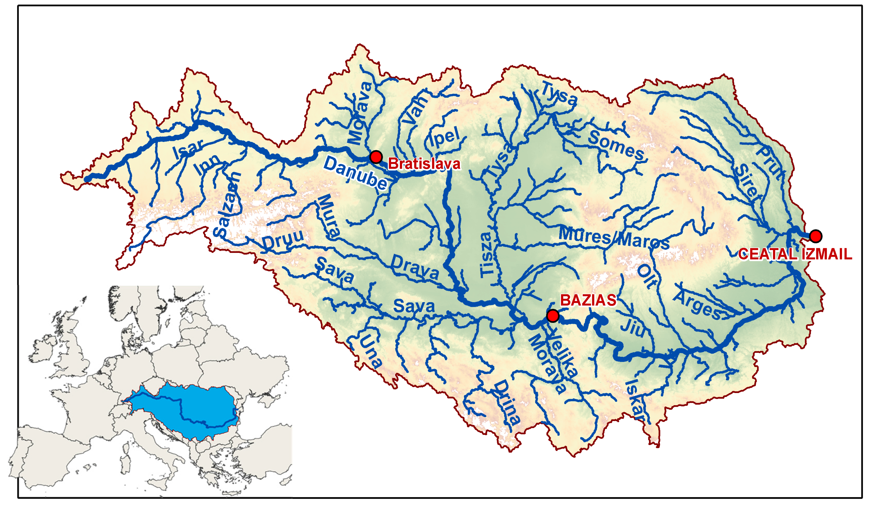
2.1. Study Region: The Danube River Basin

The Danube comprises a basin area of ~801,000 km2 and is the second largest river in Europe (~2826 km). The Danube River basin has the highest freshwater biodiversity in Europe. The habitats created by the Danube and its tributaries are home to a unique composition of species. More than 5000 animal species, including over 100 fish species, 180 breeding birds as well as 2000 vascular plants can be found in the Danube catchment [31,32]. The basin has an enormous diversity of landscapes and climates, which include high-altitude mountains, forested midland hills, upland plateaus and wet lowlands. Historically, the Danube served as a west–east corridor for species migration and recolonization between the Alpine and Mediterranean regions and the Ponto-Caspian and central Asian regions (ecoregions 417, 418) [33].
Compared to other large European rivers like the Rhine, the Danube still holds relatively large near-natural river sections with intact ecological functions [33,34]. In the river basin, about 20% of the European freshwater fish fauna are domestic (115 native species) [33]. Macroinvertebrate fauna of the Danube River are also highly diverse due to strong longitudinal and lateral hydrogeomorphic gradients. Considerable pressure on the river’s native biodiversity comes from the invasion of non-native species which threaten native species [33]. Additional pressure on riverine biodiversity comes from land use change, water stress, pollution, habitat fragmentation, extinction of former floodplains and flow regulation [33].
The Danube River can be divided into three parts. The Upper Danube, from its source to its confluence with the Morava River at Bratislava (Slovakia), is characterized by a pluvio-nival flow regime with high flow velocities and low water temperatures. The Middle Danube, ranging from Bratislava to the Iron Gate dams (Romania/Serbia) (MQ at Iron Gates 5520 m3/s), has a low elevation gradient and flows through the lowlands of the Pannonian plain. The highest annual mean precipitation (>1500 mm) occurs on the outskirts of its mountainous tributaries [35]. The Lower Danube traverses the Romanian-Bulgarian lowlands until the Danube Delta at the Black Sea. Together with the Tisza, the Sava River dominates the discharge regime in the Lower Danube, causing two seasonal maxima (spring and autumn). The annual mean discharge (MQ) of the Danube at its outlet to the Danube delta (Ceatal Izmail station) is ~6550 m3/s. The Danube River and its largest tributaries are shown in Figure 1.
The major tributary in the Upper Danube basin is the Inn River (MQ at Passau-Ingling ~735 m3/s), which more than doubles the Danube River discharge at its confluence. The Inn River basin covers parts of Austria, Germany and Switzerland. It exhibits an alpine character and a nivo-glacial flow regime. More than 800 glaciers (total area 395 km2) are located in the high alpine parts, which are shrinking due to global warming. The seasonal flow peak appears in summer due to snowmelt and heavy rains. The main tributary of the Inn is the Salzach River [33,36].
The Morava River is a left tributary of the upper Danube and enters the Danube at Bratislava (MQ 108 m3/s with flow peaks in early spring (March/April). Its catchment area covers parts of the Czech Republic, Slovakia and Austria. The meandering Morava floodplains are one of the most species-rich ecosystems in Europe, with ~12,000 different animal and plant species [33,36].
Rising in the Southern Alps in Italy, the Drava River is the dominant river in southern Austria, eastern Slovenia and Croatia. The Drava is the fourth largest (MQ 577 m3/s) of the Danube, including its major tributary Mura. It is characterized by a glacial-nival flow regime, with the highest flows during the alpine snowmelt period in May and June. Due to high precipitation in the Southern Alps, a second flow peak occurs in late autumn. The lowest flows are observed in January and February. The lower sections of Mura and Drava form a relatively free-flowing natural watercourse (~380 km) including near natural floodplains influenced by high natural water level fluctuations which bear high biodiversity [33,36].
The Tisza River is the largest sub-catchment of the Danube River (157,200 km2) and includes parts of Slovakia, Ukraine, Serbia, Romania and Hungary. It contributes ~13% to the Danube River discharge (MQ ~794 m3/s). Starting in the Carpathian Mountains as a wild mountainous stream, the Tisza changes into a braided river (slope 2‰) before entering the Hungarian plain, where it forms a meandering lowland river (slope 0.09‰). Influenced by the temperate continental climate, the Tisza is characterized by a nival-pluvial flow regime with low flows in summer and early autumn and a discharge peak in March/April. Its major sub-tributary is the Mures. The Tisza River basin is characterized by high biodiversity, higher than most western European rivers, because of its numerous (semi-)natural floodplains. More than 300 riparian wetlands are located in the basin, and the Carpathian Mountains are relatively unaffected by land use changes and management [33,36].
The Sava River is the largest tributary (MQ ~1560 m3/s) and contributes ~25% of the total discharge of the Danube River. The Sava joins the Danube at Belgrade (Serbia). Rising in the western Slovenian mountains, the Sava meanders through the Croatian lowlands. In its further course, it forms the border river between Croatia and Bosnia and Herzegovina before it flows from the Pannonian plain as a wide lowland river (channel width up to 1000 m) through Serbia. The climate of the basin is characterized as a mixture of Alpine and Mediterranean climates. As most of the river basin is located in the Alps and the Dinaric Mountains, the Sava has a nival-pluvial flow regime with a spring peak caused by alpine snowmelt. The second seasonal peak flow is induced by heavy rainfall in autumn [35]. Its major sub-tributary is the Drina River. With extended alluvial (and protected) wetlands and floodplains and a relatively natural flow regime in major river sections, the Sava basin holds numerous hotspots of biodiversity, including major protected areas and NATURA 2000 sites [33,36].
The Velika Morava River is the last significant right-hand tributary before the Iron Gate (MQ 277 m3/s). With a basin area of ~38,000 km2, it drains ~40% of the surface of Serbia. The area is dominated by a continental climate. The seasonal discharge peak occurs during the short snowmelt period in spring. The Velika Morava has extensive flood embracement to diminish the flood risk [33,36].
The Siret River originates in the northeastern Carpathian Mountains (Ukraine), but flows as a meandering river through the hilly-lowland area of the Romanian plains for most of its length. The climate of the Siret basin is temperate with a continental influence, leading to a flashy flow regime with low flows from late summer until winter and snowmelt-induced spring floods [33,36].
The Prut River is the second longest tributary (953 km) of the Danube, into which it drains just upstream of the Danube delta. Originating in the Ukrainian Carpathians, it becomes the border river between Ukraine and Romania and also between Romania and Moldova. The climate of the Prut basin is continental, leading to a flashy flow regime (MQ 110 m3/s) with a short snowmelt period in March. Major floods often occur in March, when heavy rains intensify the snowmelt peak [33,36].

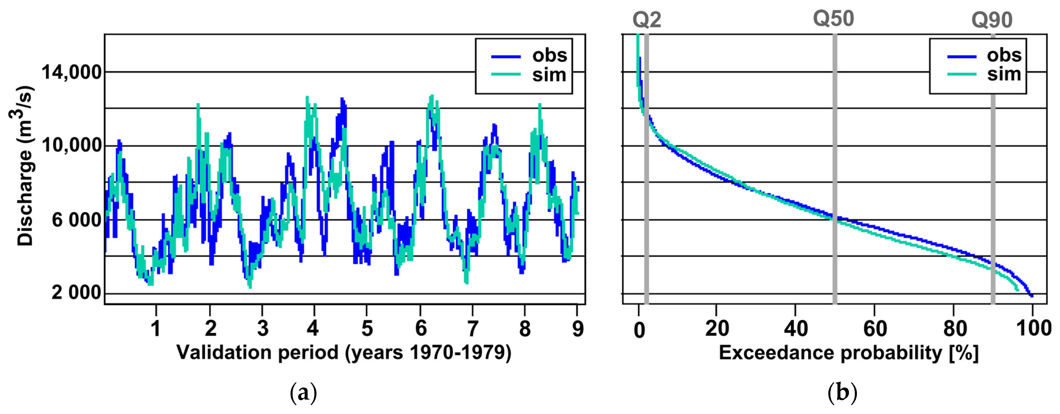
2.2. River Discharge Simulation with the Eco-Hydrological Model SWIM

The Soil and Water Integrated Model (SWIM, [30]) is an eco-hydrological model which integrates hydrological processes, vegetation and erosion on the scale of river basins using meteorological, topographical, land use, soil, vegetation and agricultural management input data as forcing datasets.
The SWIM model is semi-distributed and was specially developed for impact assessment. It comprises a three-level disaggregation scheme from basins to subbasins and to so-called hydrotopes. Hydrotopes are a hydrological concept in which areas that have the same soil, land use, elevation and subbasin type are assumed to respond hydrologically in a uniform way within one subbasin. The hydrological module is based on the water balance equation and includes four subsystems (soil surface, root zone, shallow upper aquifer and deep lower aquifer). The water balance is calculated in the hydrotopes, including percolation, return flow, capillary rise, groundwater recharge and lateral flows. Water flows in the hydrotopes are added up for each subbasin, and the lateral flows are then routed following the river network based on the Muskingum routing procedure, taking transmission losses into account. The SWIM model is driven by daily climate variables (mean, minimum and maximum air temperature, precipitation, solar radiation, and relative humidity). SWIM has been successfully applied at numerous mesoscales and large catchments for river discharge and extreme events (floods and low flows; [30]). A detailed description of the SWIM model setup and input data for the Danube river catchment is given by Stagl et al. [37].
For the Danube River catchment, the SWIM model was successfully validated and applied towards climate impact assessment [37]. The model setup for the entire Danube catchment includes 1224 subbasins and 30,807 hydrotopes. As the Danube River basin is climatically heterogeneous, it is characterized by a complex river runoff regime varying from nival in the alpine parts to mainly rain-fed in the lowlands. To account for these different river regimes of the Danubian tributaries, the SWIM model was calibrated separately for the major river subbasins. The meteorological driving data for the calibration and validation of the model were obtained from the WATCH Forcing Data [38].
The model is able to adequately simulate daily time series of river discharge for the Danube River and its major tributaries [37]. The Nash–Sutcliffe Efficiency (NSE) is above 0.6 for most of the gauges used for calibration and validation on a daily basis (and above 0.7 on a monthly basis) (Table 1). For the main stations of the Danube River, the results are “good” to “very good” [39], with a monthly NSE (NSEm) above 0.78 [37]. This also applies for the seasonality and the flow duration curve as shown in Figure 2 for the Danube River station Ceatal Izmail near the outlet to its Delta.

2.3. Climate Scenario Projections for Different Levels of Global Warming

We evaluated three climate warming scenarios, comparing the flow regime resulting from the climate during the period 1971–2000 and two future scenario periods 2031–2060 (near future) and 2071–2100 (far future). Five global climate models (GCM) from the “Coupled Model Intercomparison Project Phase 5” (CMIP5 ESMs), adequately covering the range of total GCM variation [37], were selected: HadGEM2-ES, IPSL-CM5A-LR, MIROC-ESM-CHEM, GFDL-ESM2M and NorESM1-M [40]. The outputs were bi-linearly interpolated in space to a 0.5° × 0.5° grid and bias-corrected, with a trend-preserving approach against the reanalysis WATCH dataset by the ISI-MIP project [38,40] to improve the statistical agreement with observations. They are available at a daily time-step and for the time period 1950–2099 [40].
Three different levels of global warming, or “Representative Concentration Pathways” (RCP), are simulated with each GCM. These scenarios refer to a warming level for the future period 2071–2100 (year 2085) of approximately +1.2 °C (RCP 2.6), +2.0 °C (RCP 4.5) and +3.7 °C (RCP 8.5) at a global level compared to present-day temperatures (1980–2009 average). For the period 2031–2060 (year 2045), scenarios correspond to a global warming level of approximately +1.1 °C (RCP 2.6), +1.3 °C (RCP 4.5) and +1.7 °C (RCP 8.5) compared to present-day temperatures [41]. Considering the already existing degree of warming up to the current period (1980–2009), the scenarios represent an even higher level of warming compared to pre-industrial temperatures. The local warming levels for the Danube region corresponding to the three climate scenarios are higher than the global averages and are shown in Figure A1 and Figure A2.

2.4. Eco-Hydrological Indicators of River Flow Alterations

For this study, we selected eight ecological river flow indicators which are particularly suited to being calculated from climate scenario projections (Table 2). Similar to the “Indicators of Hydrologic Alteration” approach [13,17], we compare daily mean discharges for the river sections under its “changed” (scenario) condition, with the corresponding values derived from a reference period representing the flow regime before alteration. The indicator values, except for ∆DOYpeak, show the percentage differences between the changed and the reference conditions as an average value of the simulations of the five climate models. The indicators for low and high flows are based on the long-term flow duration curve (FDC), which represents the relationship between frequency and magnitude/volume of stream flow events. The long-term FDC is most informative, as it characterizes the complete range of river discharges, from low flows to high flow events [42]. Using multi-annual daily discharge data, it displays the percentage of time per year in which specific discharge volumes are under-run or exceeded. The advantage of the FDC indicators is that they reveal changes in both the magnitude and frequency of low and high flows.
Long-term average annual river flow (∆Qyear) is often used as a basic indicator [10] and is especially relevant in lower reaches of a river [45]. The ∆Qyear is related to the size and magnitude of the river [17,21,24]. Generally, aquatic communities show distinct modifications as a function of river size [44]. These are caused, among other reasons, by changes in flow velocity and alterations in river bed gradient, and associated fining of bed sediments. Organisms sensitive to changes in velocities and bed sediment size/stability are, in particular, periphyton biomass and benthic invertebrates [21].
The river flows per season (indicators ∆QDJF, ∆QMMA, ∆QJJA, and ∆QOSN) reflect the general tendency (mean) of annual water conditions and provide a general measurement of habitat suitability [17]. Changes in seasonal means exhibit flow conditions of relative hydrological inconstancy [17]. Changes in the natural seasonal flow regime can facilitate the successful establishment of non-native species [11].
The indicator ∆DOYpeak describes changes in the long-term average day of the year with the maximum flow. Changes in the timing of high flow events impact certain life cycle requirements of many aquatic and riparian species, which are adapted to either avoid or exploit flow levels of specific magnitudes [11,17]. The natural timing of high flows provides environmental cues for initiating life cycle transitions for fish species, for example [11]. The timing of the occurrence of high flow conditions can influence the degree of stress on specific species [17].
The indicator for low flows, Q90, is the discharge level that is under-run on average during five weeks (36 days) per year. It is used, for example, as a basis to determine minimum flows in the context of water abstraction licenses [46]. At times of low flow, ecosystems are most vulnerable due to water temperature extremes and reduced dissolved oxygen concentration related to higher water temperatures, as well as reduced effluent dilution leading to deterioration in water quality [20,46]. Low flow periods impose ecological stress and are leading to a reduction in habitat availability (e.g., drying-out) and fragmentation (e.g., barriers to fish movement) [21,46].
High flows are defined in this study as Q2 levels, which are the flow levels that are exceeded on average during seven days per year. Changes in magnitude of the high flow events are likely to influence riverine and riparian species. The first ones can be affected through the intensity of habitat destruction and disturbance associated with bed movement and washout during high flow events [21]. On the other hand, many fish species can benefit from those flood and high flow events that restore river-floodplain connectivity, thus leading to an increase in abundance/biomass or enhancing recruitment [47,48,49]. Riparian plant communities are also strongly affected by the duration and depth of flooding, as revealed in a recent meta-analysis by Garssen et al. [50].

3. Results

This section presents the results for potential changes in environmental flow conditions by means of eight ecologically-relevant river flow indicators under three global warming scenarios. The maps (Figure 3, Figure 4, Figure 5, Figure 6, Figure 7 and Figure 8, Figure A3 and Figure A4) show the indicator values for major rivers in the Danube basin, including all major tributaries and the Danube River itself. In the figure columns, three global warming scenarios are shown, ranging from the lowest (RCP 2.6) to the highest (RCP 8.5) climate warming scenarios. The first row of each of these figures presents the relative changes (%) between the “near future” scenario (average of the years 2031–2060) and the reference period (average of the years 1971–2000). The second row shows the same, but for the “far future” scenario (2071–2100). The results for the indicator ∆DOYpeak are evaluated as absolute changes expressed in the number of days. All maps present changes in the multi-model mean values calculated across the simulations of five driving GCMs.

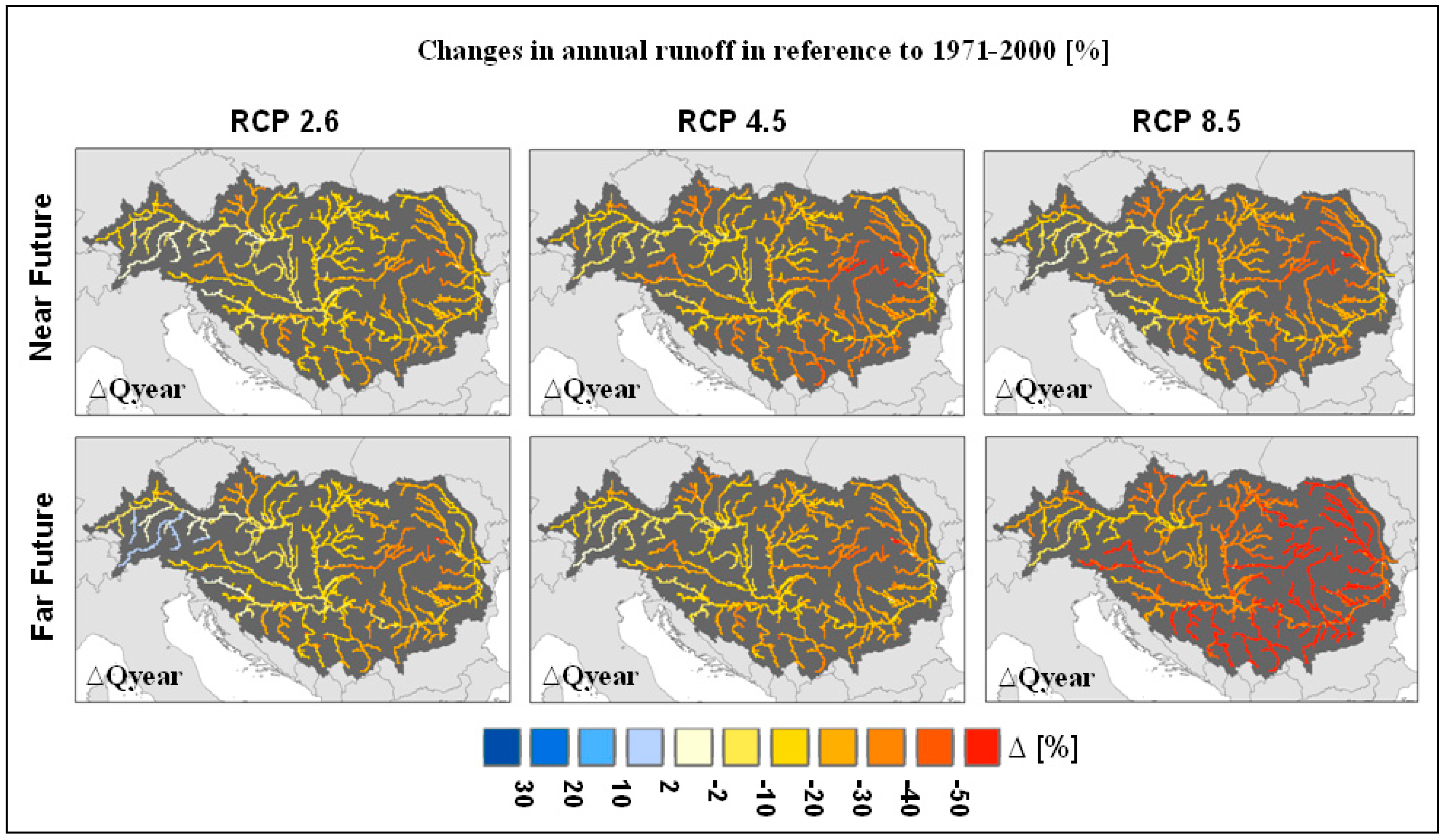
3.1. Climate Change Impacts on Long-Term Annual Average Discharge

The results for ∆Qyear (Figure 3, Table 3) show that climate change may lead to a decrease in annual river discharge in all rivers in the Danubian basin, except for the alpine rivers Lech and Isar and, in particular, the Inn River. For the Inn River, no changes or even a slight increase (RCP 2.6 for 2071–2100) are projected for the near future (Figure 3). Most affected by the decrease (∆Qyear > −30%) are the tributaries of the Lower Danube basin, as well as rivers originating in the Carpathian (in particular Mures and Olt Rivers) and Dinaric Mountains. The results also show a strong decrease for the headwaters of the Drava River, with maximum ∆Qyear values of −18% to −30% (near future) and −12% to −48% (far future). For the lower Sava River (station Sremska Mitrovica), the annual runoff is projected to decrease by 24% to 36% (∆ 2031–2060) and 22% to 58% (∆ 2071–2100). For the Tisza River, the projected decrease in annual river flow is less distinct (∆Qyear values > −9%), except for the far future under RCP 8.5 with ∆Qyear of −25% (lower reach station Sziged). Under RCP 8.5 for the far future, a very strong decrease is projected for the rivers in the Middle and Lower Danube catchment (>40%) and a strong decrease of 10%–30% in the Upper Danube basin as well as in the Pannonian lowlands. The Qyear of the Danube river at its outlet to the delta is projected to change only slightly due to climate warming until mid-century (∆Qyear: −5% to −8%). For the far future, the changes in Qyear are accelerating for the Lower Danube River from 3% (RCP 2.6) to 19% (RCP 8.5).

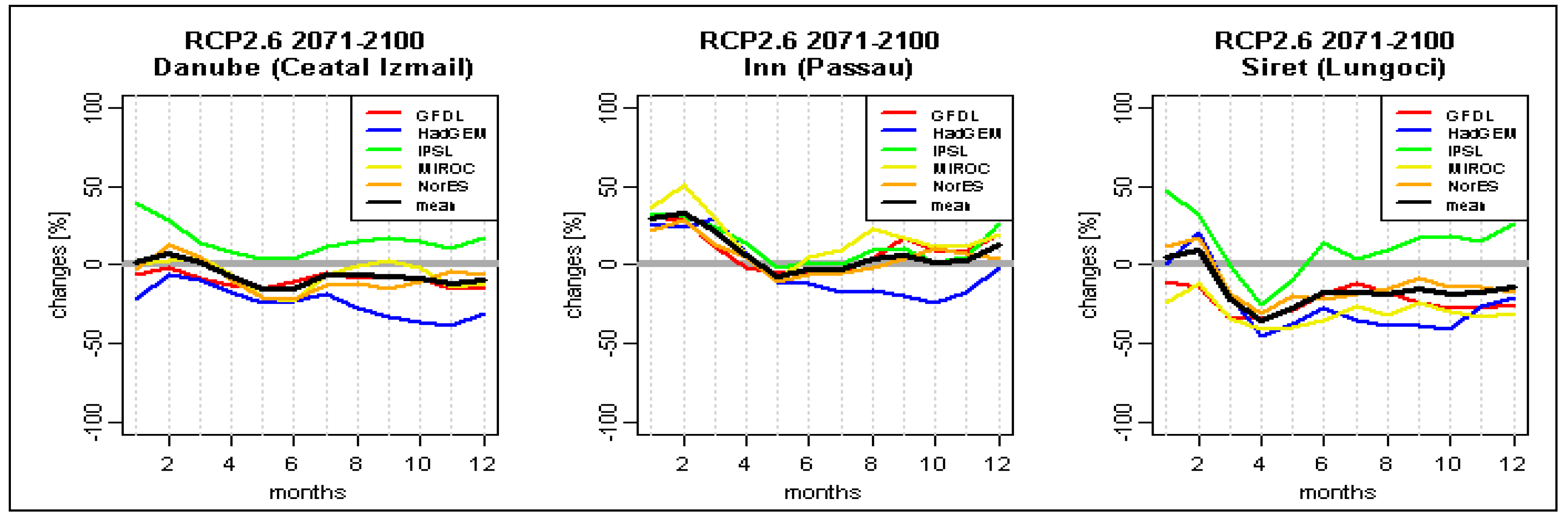
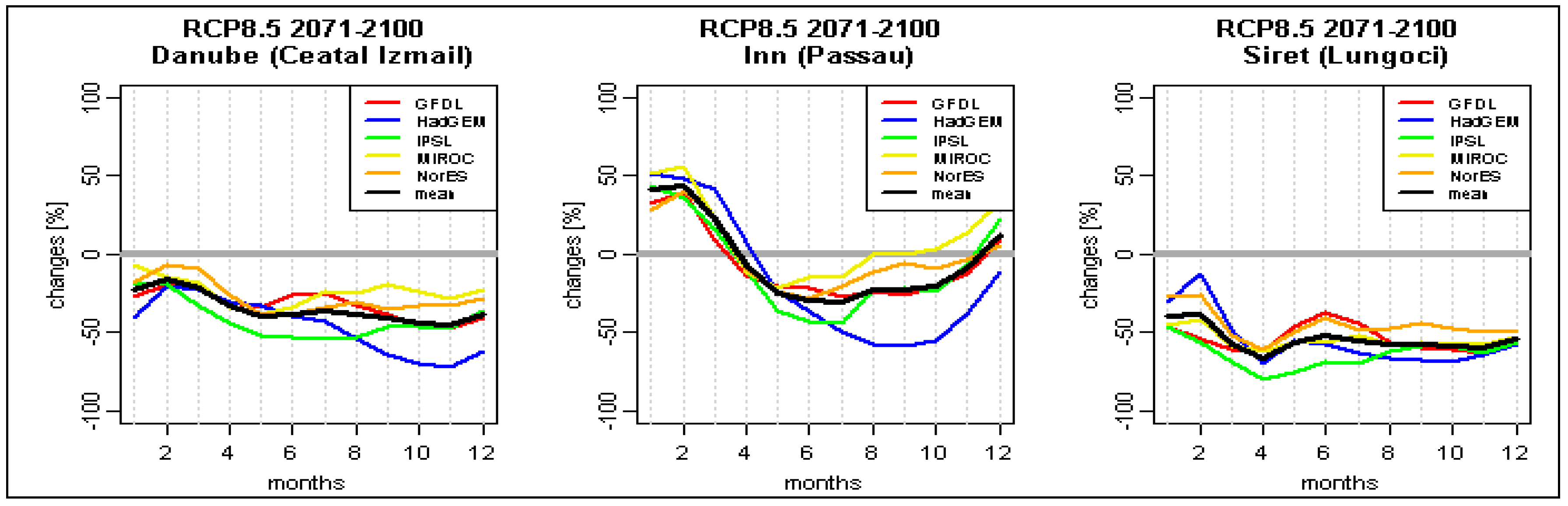
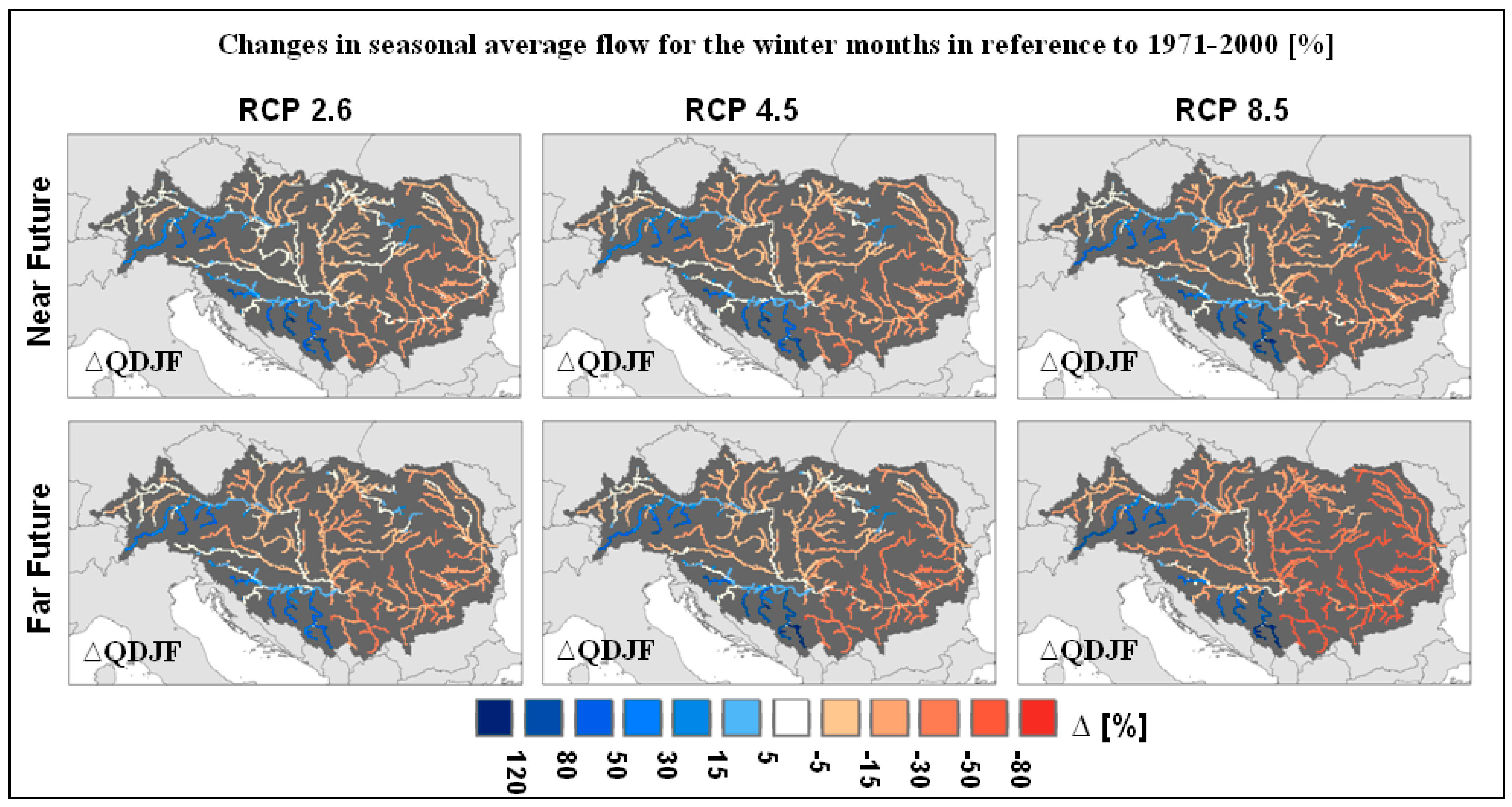
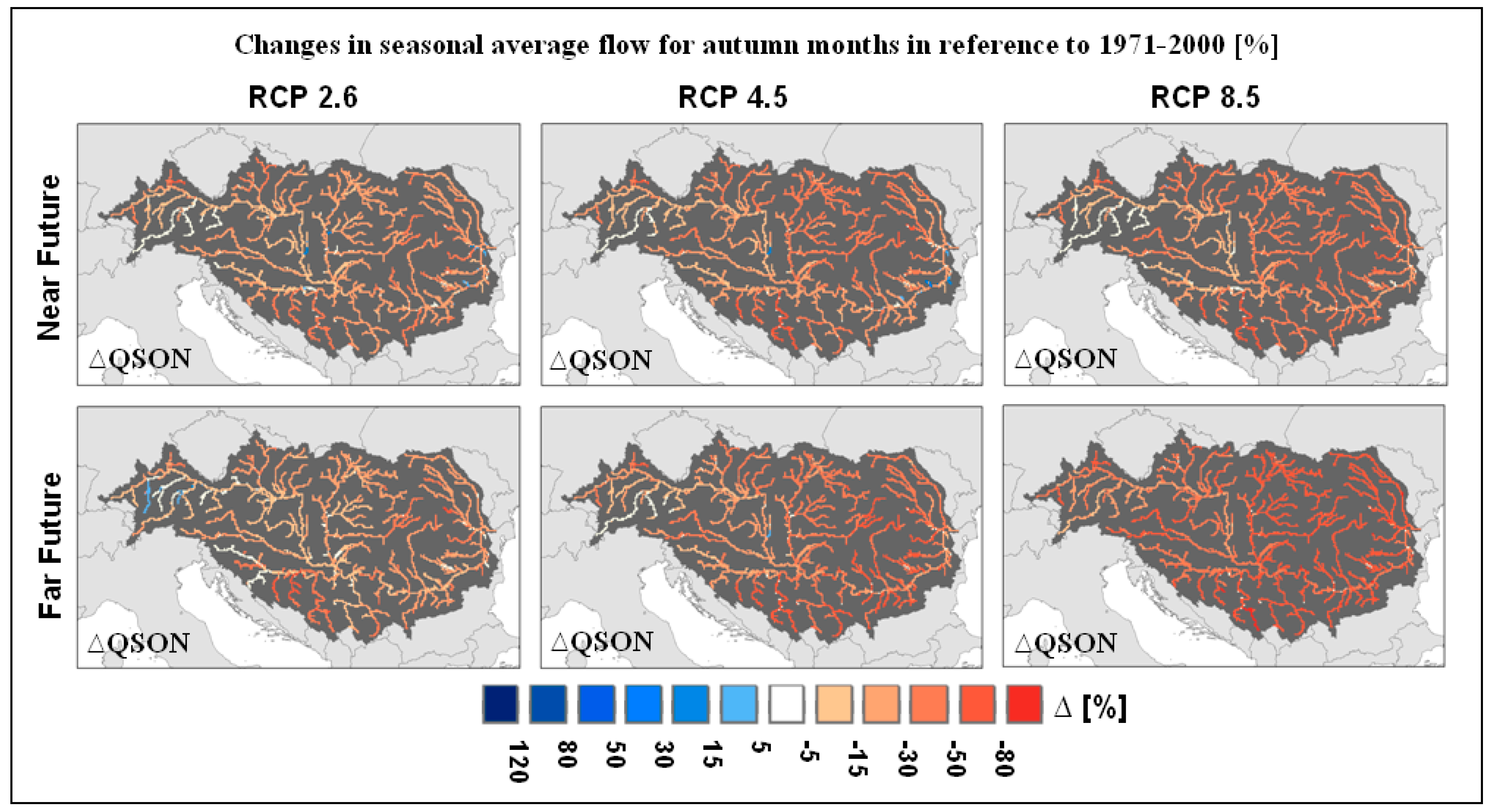
3.2. Climate Change Impacts on the Seasonal Regime

The seasonal flow regime in the Danube River catchment is projected to change significantly with increasing global temperatures (see indicators ∆QDJF (Figure 4), ∆QMMA (Figure A3), ∆QJJA (Figure 5), and ∆QOSN (Figure A4) and Table 3). Except in a few tributaries for the winter months, the seasonal discharge of the rivers in the Danube basin is projected to decline progressively with global warming. The most affected by this decrease (in relative terms) are the tributaries of the Lower Danube basin, the Mures River, the headwaters of the Drava River, and the Dinaric tributaries of the Sava and Morava Rivers. For autumn (∆QOSN), the results show the strongest decrease in seasonal runoff out of all the seasons. However, the decrease in summer discharge is more severe, as it aggravates existing low flow periods. For the winter months, rivers originating in higher mountain regions show an increase in average river runoff, in particular the alpine tributaries of the Upper Danube basin (Inn River: ∆QDJF 19% to 31% and Enns River: ∆QDJF > 50%) and the high mountain tributaries of the Dinaric Mountains (∆QDJF > 50%). Such increasing winter discharges are caused by changes in snow regime and higher winter precipitation, which is not compensated by higher evaporation demand. The QDJF increase in the Inn and Enns Rivers is leading to an increased projected winter discharge for the Upper Danube (Bratislava station) of 6 to 14%. In addition, the winter runoff of the Sava River is projected to increase by 11% to 15% in the near future. For the far future, the increase in QDJF, e.g., for the lower Sava (Sremska Mitrovica station) is getting less distinct with increasing global temperatures (RCP 2.6: 20%; RCP 4.5: 15%, RCP 8.5: 1%).
The results for the Danube River at Iron Gate are very similar to those for the Danube River at its outlet to the delta and show a decrease in river discharge for all seasons. In the winter months, the projected decrease is the lowest of all seasons (∆QDJF < 12%, except RCP 8.5 for the far future: ∆QDJF: −25%). The strongest relative decrease for the Danube River discharge is projected for the autumn season (9% to 43%), but is still distinct for summer (9% to 37%) and spring (8% to 31%) depending on the climate warming scenario.

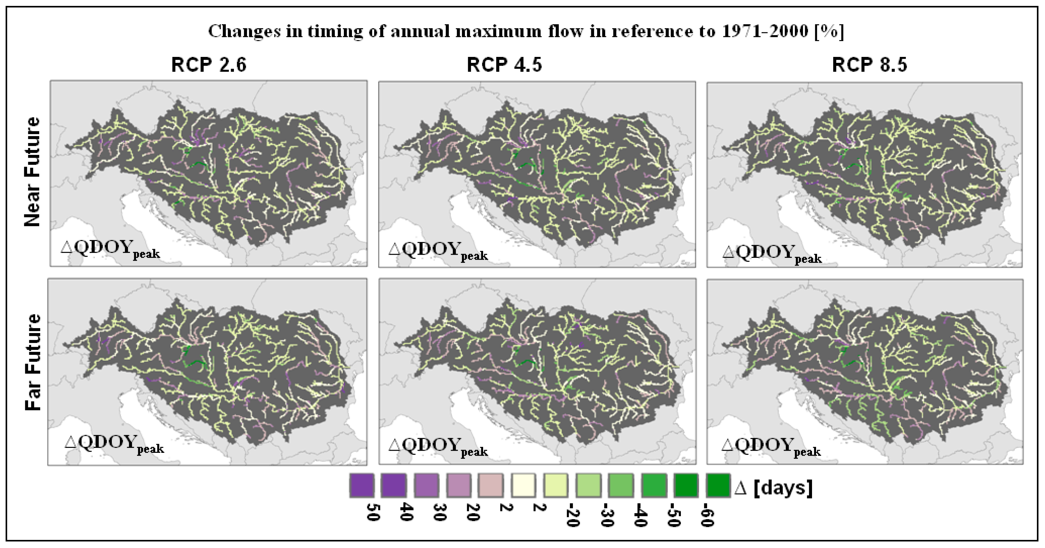
3.3. Climate Change Impacts on Timing of Annual Peak Flow

The results for the ∆DOYpeak (Figure 6 and Table 4) indicate that the timing of the annual maximum flow might shift considerably with climate warming. For most parts of the Upper Danube basin, the annual peak flow is projected to occur (slightly) earlier in the year, but later in the alpine rivers (Lech, Isar, Upper Inn, Salzach, Enns) by up to one month depending on the scenario. Shifts in the timing of the annual peak flow are mostly related to the reduced storage of winter runoff due to changes in snow regime (e.g., earlier snowmelt and a rise of the snow line) and/or changes in the precipitation patterns. After the confluence of the Danube with the Morava River, the peak flow is projected to occur earlier (by 10 to 21 days). The timing of the annual peak flow of the Danube River at Bratislava shows barely any changes for the near future (of less than 6 days), but in the far future, peak flow may occur up to two weeks (16 days) later. The results for the Tisza River indicate a shift in the high flow peak from the end of March to the beginning of March. Most parts of the Carpathian rivers are projected to peak earlier (up to ∆DOYpeak > −30 days). In addition, the peak flow of the Sava is projected to occur earlier, shifting from mid- to the beginning of April. At the end of the 21st century, under the global warming scenarios RCP 4.5 and 8.5, the Sava River’s peak flow is projected to occur around one month later in the year, which may mainly be caused by changes in the alpine headwaters. The Velika Morava River, originating in the Dinares, is projected to peak later in the year, shifting progressively from February to March. The DOYpeak for the Danube River before the delta is projected to shift progressively from the end of April to the beginning of April in the near future and to the end of March in the far future.

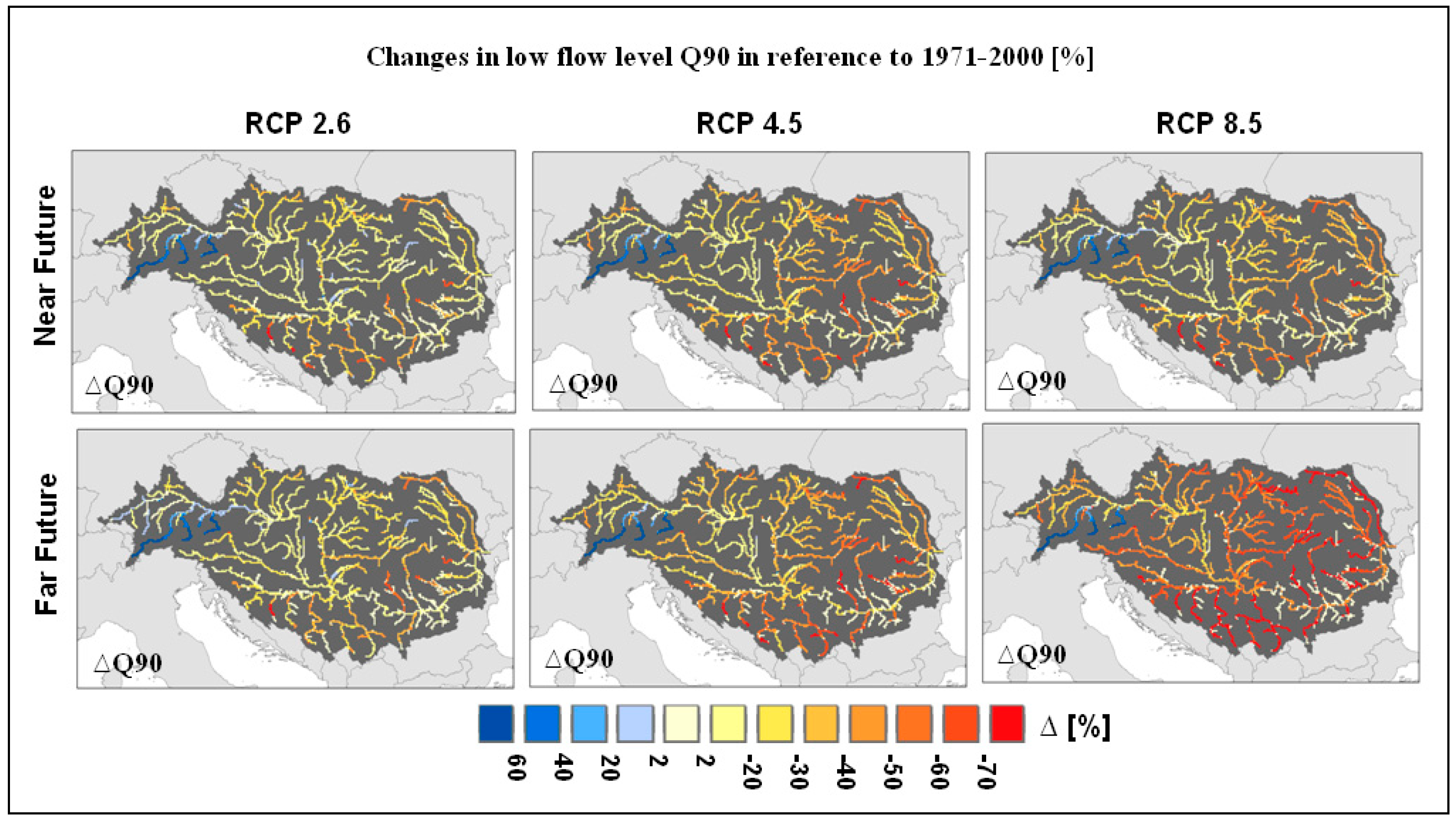
3.4. Climate Change Impacts on Long-Term Statistical Low Flows

The ∆Q90 indicator values, as expressed in percent changes from recent conditions, are more sensitive to relative changes in the flow magnitude than, e.g., ∆Q2 values for high flow, because the reference absolute values for low flow magnitudes are smaller. With accelerating global warming, the results show that low flow levels in the Danube River catchment gradually decrease, except in the rivers of the Northern Alps, where low flow magnitudes are increasing (by more than 20%) under all scenarios for the near and far future (Figure 7 and Table 3). Under the RCP 2.6 warming scenario for most rivers in the Danube basin, no or only small changes in low flows are projected for the near future. Under the RCP 4.5 scenario, a strong decrease in Q90 levels (of up to 40%) is simulated, in particular for the Sava and Morava Rivers and tributaries in the Mediterranean Lower Danube basin. Under the RCP 8.5 scenario, a very distinct decrease in low flow volume (of up to 50%) is projected for the whole Danube region for the end of the 21st century, except for the Inn and Enns Rivers, where the Q90 low flow levels are projected to increase. Recent low flow levels in the Danube River outlet to the delta, which are under-run 36 days a year (Q90), might not be reached on 62 days out of the year (RCP 2.6) in the near future (RCP 4.5: 46 days; RCP 8.5: 73 days), and 51 days in the far future (RCP 2.6) (RCP 4.5: 87 days; RCP 8.5: 128 days). Hence, in the RCP 8.5 world, the Q90 low flow levels at the Lower Danube River might correspond to recent Q99 levels (4 days/year) in the far future.

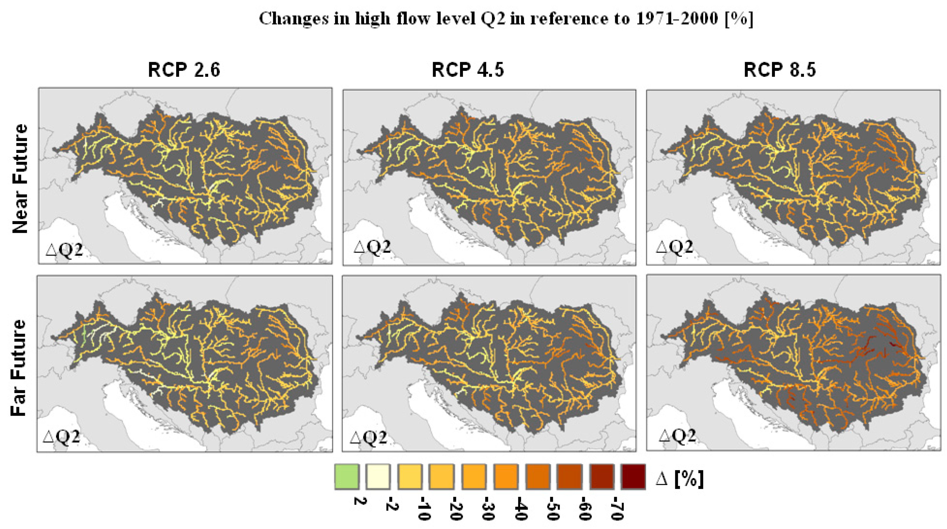
3.5. Climate Change Impacts on Long-Term Statistical High Flows

A reduction in high flow levels (Q2) is projected for almost all rivers in the Danube basin under all scenarios due to climate warming (Figure 8 and Table 3). The strongest decrease is projected for the Morava River and Danubian tributaries originating in the Carpathian Mountains, the Lower Danube basin and in the Dinaric mountain region. Under the RCP 2.6 scenario, high flow levels are projected to remain relatively unchanged for the northern alpine rivers Isar, Lech and Inn for the near and far future. For the Danube River at the entrance to its delta, a moderate reduction in high flows (9% to 16%) is projected, which remains relatively homogeneous over the RCP scenarios and both future periods. Hence, the Q2 discharge levels of the Lower Danube for the future periods correspond to recent Q4 to Q6 levels. In addition, recent Q2 magnitudes are projected to occur less frequently than every year due to climate warming. For the lower Sava River (Sremska Mitrovica station), changes in the ∆Q2 indicator depend on the selected warming scenario and show a decrease in high flow volume of 8% to 14% for the near future and 8% to 24% for the far future. Hence, future Q2 levels (7 days/year) of the Sava correspond to values which are nowadays reached at Q3 (RCP 2.6) (11 days/year) to Q7 (RCP 8.5, 2071–2100) (25 days/year). High flow magnitudes of the lower Tisza River (Szeged station) are also projected to decrease strongly, with a reduction in Q2 levels of 15% to 25% in the near future and 19% to 33% in the far future. High flow magnitudes, which might be exceeded in the future on seven days per average year at the Lower Tisza, correspond to flow volumes which nowadays appear 15 days out of the average year (RCP 2.6 and RCP 4.5, for 2031–2060) or even 40 days a year (RCP 8.5, for 2071–2000).

4. Discussion

In this study, we evaluated the impact of climate change on ecological river flow alterations for the Danube River and its major tributaries. The use of eco-hydrological indicators to exhibit alterations in the environmental flow regime should bridge the gap between hydrology and riverine ecology. We presented projected changes for eight environmental flow indicators under three climate warming scenarios, pointing to a global temperature increase by the end of the 21st century of ~2 °C (RCP 2.6), ~3 °C (RCP 4.5) or ~4 °C (RCP 8.5) compared to pre-industrial times.
The results reveal that climate change is projected to significantly alter the recent environmental flow regime in the Danube River basin, especially in the tributaries of the Middle and Lower Danube basin. The impacts strongly accelerate with increasing global temperatures. Under the RCP 2.6 scenario, the projected environmental flow alterations might still be moderate for most of the rivers. Under the RCP 4.5 scenario, however, the results show very distinct changes for most of the eco-hydrological indicators. Finally, under the high-end RCP 8.5 warming scenario, the recent ecological flow regime might be highly altered, especially in all tributaries of the Middle and Lower Danube basin. The greatest changes are associated with a discharge reduction in the summer half of the year, including a very critical decrease in low flow magnitudes (Sava, Drava, and Tisza Rivers and all tributaries of the Lower Danube basin). The Velika Morava River in particular is affected by a very strong decrease in low flow magnitudes and a strong decrease in winter flow. For the Tisza River, the results also reveal, apart from a distinct decrease in low flow magnitudes, a strong decrease in high flow magnitudes. The impacts on the Danube River in its lower reaches are not so distinct compared to those of its (smaller) tributaries (except for the RCP 8.5 scenario), mainly due to its large volume of river runoff throughout the year. For the tributaries of the Upper Danube basin, the projected impacts do not increase as dramatically as they do for the Middle and Lower basin with increasing global warming. For the rivers of the Upper Danube basin, the largest alterations are projected for winter flows, due to a projected increase in winter precipitation and changes in the snow regime. For the Alpine areas, a strong decrease in low flow magnitudes and distinct changes in the timing of the annual maximum flow are also projected. The largest impacts in the Upper Danube basin are projected for the Morava River, with a strong decrease in high and low flow magnitudes, especially in the summer months. The Danube River in its upper part (Bratislava station) is relatively less impacted under the RCP 2.6 and RCP 4.5 scenarios, but for the RCP 8.5 the summer discharge is projected to decrease significantly.

4.1. Ecological Implications of Projected Alterations in the Environmental River Flow Regime

Future climate change is projected to cause moderate to large shifts in the flow regimes of the Danube River and its tributaries, hence shifting environmental niches for biota with adverse consequences for freshwater ecosystems. The “habitat template”, to which actual riverine species in the Danube catchment are adapted, is formed by the rivers’ recent flow regime. Alterations to this “natural regime” are changing the organizing role of river flows through the dynamically varying physical environment of these habitats [11]. Changes in the hydrological regime may create new conditions to which native biota may be poorly adapted and exceed the tolerances of some aquatic biota and riparian plants [51]. Additionally, changes in the “natural flow regime” could facilitate the successful establishment of non-native species [11]. This would increase the pressure on the native species in the Danube riverine habitats, where already nowadays 40% of the species are invasive [33]. In their review of 165 studies on aquatic or riparian responses to flow regime alteration, Poff and Zimmermann [7] found that all changes in the flow regime may impact in-channel and riparian ecosystems, while the majority of ecological changes were reported to altered flow magnitudes. Ecological responses of fish to both elevated and reduced flow magnitudes were largely reported as decreases, while macroinvertebrates showed mixed responses to increasing or decreasing flow magnitudes [7]. It remains an unsolved question just how much change from the natural range of flow variability is still acceptable for sustaining adjusted aquatic ecosystems and species [52]. The “Indicators of Hydrologic Alteration” approach given by Richter et al. [13] includes a “Range of Variability” analysis which allows effective comparison of the pre- and post-impact conditions, but does not pose any ecologically grounded quantitative limit values. Although some authors propose thresholds for a set of selected indicators of hydrological alterations (e.g., [3,6,25]), simple rules for thresholds are likely to be misleading as the biological impact of flow alterations also relies on other ecological factors like habitat quantity and quality [52].
Projected changes to the natural flow regime affect aquatic organisms both directly and indirectly. Reductions in flow magnitude, as widely projected for the Danube River and its tributaries, are associated with a decrease in flow velocity, water depth and wetted width, water temperature increase and changes in bed sediment size and stability [21,53,54]. This may lead to changes in habitat diversity and the availability of food resources, such as algae and organic matter [53]. Projected shifts in the timing of flow events in the Danube catchment, like annual maximum discharge, can be critical for riverine species which are timed to either exploit or avoid flows of specific flow magnitudes for their life cycle transitions, such as spawning, larval emergence and egg hatching [11,20]. Climate change is expected to impact the snow cover, including its buffering function for the runoff regime, especially in higher elevations of the Danube basin. Hence, winter precipitation will in part not be stored in snow pack and released during snowmelt. Earlier snowmelt-induced floods are reducing the retention time of sediments and organic matter, thereby influencing the availability of nutrients and microhabitats in the rivers [20]. Additionally, earlier snowmelt or no snow cover during winter may lead to an earlier and longer rise in water temperature, impacting species which are sensitive to changes in this variable [45]. Riverine ecosystems are most vulnerable at times of low flows (“bottlenecks”), exerting selective pressure on some species [7], especially if critical flow levels <Q95 (18 days/year) increase in the future. Projected decreases in low flow magnitudes in the Danube catchment may lead to exacerbated habitat destruction, degradation or fragmentation for riparian species, concentration of aquatic organisms and a reduction of plant cover. A prolongation of low flows as projected for the summer months in most parts of the basin is also associated with water temperature extremes, especially in combination with projected higher air temperatures, reaching, e.g., lethal limits for some fish species, with reduced dissolved oxygen, deterioration in water quality and reduced flow velocity including a reduction in shear stress [11,20,54]. Changes in high flows, which are projected to decrease in most rivers in the Danube basin, may influence the composition and relative diversity of existing species [11]. High flows are associated with sediment transport in the river bed, exporting organic resources, rejuvenating the biological community and allowing species with fast life cycles to reestablish themselves [11].

4.2. Comparison of the Results to Other Available Studies

For the Danube River and its tributaries, only a few studies are available that focus on the future impacts of climate change on ecologically relevant river flow characteristics. Laizé et al. [6] quantified the degree of flow regime alterations on a pan-European scale in terms of ecologically relevant flow indicators for the middle of the 21st century. They identified similar patterns in the Danube basin as found in our results, including a zone of “highest risk” in the southwestern part of Eastern Europe under the SRES A2 scenario. This zone of “highest risk” includes the Morava River, the Vah, the Tisza, the main parts of the Sava, the Velika Morava River, and all the tributaries of the Lower Danube basin.
Schneider et al. [16] evaluated the impacts of climate change on natural flow regimes on the European scale (0.5° resolution) by the 2050s under the A2 emission scenario using the global hydrology model WATERGAP3. Quantifying projected flow alterations with the “Indicators of Hydrological Alteration” approach, their results showed “remarkable” flow modifications for European rivers. Similar to our findings, they ranked the impact of climate change on the flow regime as “medium” for the Danube River itself, as well as for the tributaries of the Upper Danube basin. For the tributaries of the Middle Danube basin, including the Sava and Tisza, they classified the projected alterations as “medium” to “severe”, and as “severe” impacts for the rivers in the Lower Danube basin.
Lobanova et al. [22] carried out a small scale modeling study for a Carpathian headwater of the Mures River, analyzing different “Indicators of Hydrological Alteration” by [17] under an ensemble of various climate models (A1B). Similar to our results, they found a model agreement for a projected increase in winter discharge, a decrease in summer and late spring flows, as well as a prolongation of low flow periods until the end of the 21st century. While our results indicate a decrease in high flow magnitudes in this area, Lobanova et al. [22] found a slight increase in median values for the duration of high flow events, but no model agreement for the number of high flow events per year.

4.3. Potential Sources of Uncertainty in the Eco-Hydrological Impact Modeling Chain

Uncertainties in the projections of future river runoff arise from different sources in the hydro-climatic modeling chain. When simulating future river flows, the driving GCM forcing was found to have the largest contribution to the overall modeling uncertainty [55,56]. Thompson et al. [27] reported considerable inter-GCM differences in the risk of ecological impact in their climate change impact assessment on environmental flows in the Mekong River basin. In this study, bias correction adds an additional factor of uncertainty, while giving a better representation of the recent climatic conditions. Until the middle of the 21st century, the choice of the RCP scenario generally has less influence than the GCM on the results, but the warming scenario becomes much more dominant until the end of the century (by scenario definition).
Climate models are often not optimized to adequately represent the spatial and temporal variability of the meteorological variables required to account for the occurrence and dynamic of extreme hydrological conditions on regional scales [57]. Hence, when selecting the eco-hydrological indicators for this study, we focused on indicators that can be replicated reasonably well by both the hydrological model and the driving climate models, e.g., by avoiding single threshold values and extremes. Furthermore, all selected indicators were calculated as mean values for 30-year periods, considering that climate models are optimized to represent long-term climatic conditions [58]. The hydrological model and its parameterization additionally contribute to the overall uncertainty [56,59]. Uncertainty related to the hydrological model is significantly less important compared to the uncertainty resulting from a large number of climate scenarios [56,60].
The five selected GCMs adequately cover the spectrum of CMIP5 climate models as used in the AR5 IPCC report [37]. We used the ensemble mean values of these GCMs for our results shown in Figure 3, Figure 4, Figure 5, Figure 6, Figure 7 and Figure 8, and Figure A3 and Figure A4, which was found to perform better than individual climate models in terms of systematic bias and to be less prone to featuring large deviations for particular regions [61]. Nevertheless, the ensemble mean value partly disguises the uncertainties related to the choice of the driving climate model. The ensemble mean value may in particular generate a “false sense of security” if the GCM models disagree in the direction of change, which occurs in the Danube catchment area in particular for transition periods like spring and autumn (see Figure 9). In the Upper Danube basin, the climate change signal is quite strong for the winter and summer seasons. For the Middle and Lower Danube basin, the highest deviations in the climate change signal arise for winter runoff. Such deviations between the GCMs in the projected amount of precipitation arise, among other causes, due to the location in a climatic transition zone of southeastern Europe [37].
In this study, we focused on impacts due to changes in the climatic drivers of river runoff, while keeping other factors constant, like land use patterns, for example, which also influence the hydrological regime. In the simulation, we also did not include water management, which might have a certain buffering effect [62], and water withdrawals, e.g., for irrigation, which might partly aggravate the future low flow situation.

5. Conclusions

This study has provided a regional overview of the potential impacts of climate change on ecologically relevant river flow alterations in the Danube River and its major tributaries up to the end of the 21st century under three different global warming scenarios. Applying the regional eco-hydrological SWIM model, changes in river flow regimes were quantified at a high spatial resolution using eight environmental flow indicators. This is the first climate impact assessment for ecologically relevant flow indicators with a regional hydrological model covering the whole Danube river basin and, hence, the entire Danube River until its outlet into the delta.
Climate change is expected to distinctively alter ecologically important attributes of the flow regimes in the Danube River catchment and, hence, to become an additional powerful stressor for riverine ecosystems on top of existing human stressors. Particularly affected are the tributaries in the Middle and Lower Danube basin, where many river sections, e.g., in the Carpathian Mountains, at present still retain a relatively natural flow regime and ecosystems barely affected by human interventions [33].
Changes in river flow regime as a consequence of climate change will occur gradually, unlike the abrupt changes resulting from water management [20]. The projected impacts strongly accelerate if global mean temperatures rise more than 2 °C compared to pre-industrial times. Especially under medium (RCP 4.5) and high (RCP 8.5) warming scenarios, the capacity for ecosystems and their species to adapt to new habitat conditions will most likely not be sufficient to cope with projected magnitudes of climate change without a substantial loss in riverine species and ecosystem services in the second half of the 21st century [4]. Climate change will exacerbate already existing anthropogenic pressures on riverine ecosystems from, e.g., land use change, as well as channelization, dams and water withdrawals [4,20].
To assess the impact of climate change on riverine ecosystems due to river flow alterations in a quantitative way would be highly relevant for the protection of these ecosystems. There exists a great need for a better understanding of the ecological response of riverine species to different degrees of alterations in river flow regimes [14], in particular ranges of variability of flow indicators, which still enable the functioning of existing ecosystems. The achievement and prospective maintenance of a “good ecological status” of the Danube River and its tributaries, as required by the European Water Framework Directive, might in the future also depend on the development of adaptive environmental management to climate-driven alterations in river flow regimes. Importantly, this adaptive management should be different for natural and semi-natural river sections, in which the main focus should be on limiting flow alterations than on modified and managed sections, in which “new” flow regimes should be designed in order to achieve specific ecological and ecosystem service outcomes [63]. In view of the fact that the issue of climate change has been rather overlooked in the recent EU policy documents on ecological flows [3], this study is a valuable contribution informing policymakers on climate-driven threats to riverine ecosystems in the largest EU river basin.

Acknowledgments

We acknowledge the Global Runoff Data Centre (GRDC, 56068 Koblenz, Germany), which provided the historical discharge data. We thank the ISI-MIP project for the provision of bias-corrected climate scenarios. This study was carried out within the framework of the HABIT-CHANGE project, which was implemented through the CENTRAL EUROPE program co-financed by the European Regional Development Fund (ERDF). We especially acknowledge also the reviewers for the valuable contributions to the manuscript.

Author Contributions

This study was carried out by Judith C. Stagl under the supervision of Fred F. Hattermann.

Conflicts of Interest

The authors declare no conflict of interest.

Appendix A

Figure A1. Projected changes in daily mean surface air temperature for the winter half-year (October–March) in the Danube basin in reference to 1971–2000 [%] for different levels of global warming (RCP 2.6, RCP 4.5 and RCP 8.5). The first row shows the absolute changes up to the near future scenario period (2031–2060), and the second row up to the far future scenario period (2071–2100).
Water 08 00566 g010
Figure A2. Projected changes in daily mean surface air temperature for the summer half-year (April–September) in the Danube basin in reference to 1971–2000 [%] for different levels of global warming (RCP 2.6, RCP 4.5 and RCP 8.5). The first row shows the absolute changes up to the near future scenario period (2031–2060), and the second row up to the far future scenario period (2071–2100).
Water 08 00566 g011
Figure A3. Projected changes in autumn river discharge (∆QSON) for the major rivers in the Danube basin in reference to 1971–2000 [%] for different levels of global warming (RCP 2.6, RCP 4.5 and RCP 8.5). The first row shows the relative changes up to the near future scenario period (2031–2060), and the second row up to the far future scenario period (2071–2100).
Water 08 00566 g012
Figure A4. Projected changes in spring river discharge (∆QMMA) for the major rivers in the Danube basin in reference to 1971–2000 [%] for different levels of global warming (RCP 2.6, RCP 4.5 and RCP 8.5). The first row shows the relative changes up to the near future scenario period (2031–2060), and the second row up to the far future scenario period (2071–2100).
Water 08 00566 g013

References

  1. Eisele, M.; Steinbrich, A.; Hildebrand, A.; Leidundgut, C. The significance of hydrological criteria for the assessment of the ecological quality in river basins. Phys. Chem. Earth 2003, 28, 529–536. [Google Scholar] [CrossRef]
  2. Acreman, M.C.; Ferguson, A.J.D. Environmental flows and the Euopean Water Framework Directive. Freshw. Biol. 2009, 55, 32–48. [Google Scholar] [CrossRef]
  3. European Commission. Ecological Flows in the Implementation of the Water Framework Directive; Technical Report—2015-086; Environment: Brussels, Belgium, 2015; p. 108. [Google Scholar]
  4. Settele, J.; Scholes, R.; Betts, R.; Bunn, S.; Leadley, P.; Nepstad, D.; Overpeck, J.T.; Taboada, M.A. Terrestrial and inland water systems. In Climate Change 2014: Impacts, Adaptation, and Vulnerability. Part A: Global and Sectoral Aspects. Contribution of Working Group II to the Fifth Assessment Report of the Intergovernmental Panel on Climate Change; Field, C.B., Barros, V.R., Dokken, D.J., Mach, K.J., Mastrandrea, M.D., Bilir, T.E., Chatterjee, M., Ebi, K.L., Estrada, Y.O., Genova, R.C., et al., Eds.; Cambridge University Press: Cambridge, UK; New York, NY, USA, 2014; pp. 271–359. [Google Scholar]
  5. Dudgeon, D.; Arthington, A.H.; Gessner, M.O.; Kawabata, Z.-I.; Knowler, D.J.; Lévêque, C.; Naiman, R.J.; Prieur-Richard, A.-H.; Soto, D.; Stiassny, M.L.J.; et al. Freshwater biodiversity: Importance, threats, status and conservation challenges. Biol. Rev. 2006, 81, 163–182. [Google Scholar] [CrossRef] [PubMed]
  6. Laizé, C.L.R.; Acreman, M.C.; Schneider, C.; Dunbar, M.J.; Houghton-Carr, H.A.; Flörke, M.; Hannah, D.M. Projected flow alteration and ecological risk for pan-European rivers. River Res. Appl. 2014, 30, 299–314. [Google Scholar] [CrossRef] [Green Version]
  7. Poff, N.L.; Zimmermann, J.K.H. Ecological responses to altered flow regimes: A literature review to inform the science and management of environmental flows. Freshw. Biol. 2010, 55, 194–205. [Google Scholar] [CrossRef]
  8. Döll, P.; Zhang, J. Impact of climate change on freshwater ecosystems: A global-scale analysis of ecologically relevant river flow alterations. Hydrol. Earth Syst. Sci. 2010, 14, 783–799. [Google Scholar] [CrossRef] [Green Version]
  9. Arthington, A.H.; Naiman, R.J.; McClain, M.E.; Nilsson, C. Preserving the biodiversity and ecological services of rivers: New challenges and research opportunities. Freshw. Biol. 2010, 55, 1–16. [Google Scholar] [CrossRef]
  10. Bragg, O.M.; Black, A.R.; Duck, R.W.; Rowan, J.S. Approaching the physical-biological interface in rivers: A review of methods for ecological evaluation of flow regimes. Prog. Phys. Geogr. 2005, 29, 506–531. [Google Scholar] [CrossRef]
  11. Poff, N.L.; Allan, D.J.; Brain, M.B.; Karr, J.R.; Prestegaard, K.L.; Richter, B.D.; Sparks, R.E.; Stromberg, J.C. The natural flow regime: A paradigm for river conservation and restoration. Bioscience 1997, 47, 769–784. [Google Scholar] [CrossRef]
  12. Richter, B.D.; Baumgartner, J.V.; Braun, D.P.; Powell, J. A spatial assessment of hydrologic alteration within a river network. Regul. Rivers Res. Manag. 1998, 14, 329–340. [Google Scholar] [CrossRef]
  13. Richter, B.D.; Baumgartner, J.V.; Wigington, R.; Braun, D.P. How much water does a river need? Freshw. Biol. 1997, 37, 231–249. [Google Scholar] [CrossRef]
  14. Arthington, A.H.; Bunn, S.E.; Poff, N.L.; Naiman, R.J. The challenge of providing environmental flow rules to sustain river ecosystems. Ecol. Appl. 2006, 16, 1311–1318. [Google Scholar] [CrossRef]
  15. Acreman, M.C.; Dunbar, M.J. Methods for defining environmental river flow requirements—A review. Hydrol. Earth Syst. Sci. 2004, 8, 861–876. [Google Scholar] [CrossRef]
  16. Tharme, R.E. A Global Perspective on Environmental Flow Assessment: Emerging Trends in the Development and Application of Environmental Flow Methodologies for Rivers. River Res. Appl. 2003, 19, 397–441. [Google Scholar] [CrossRef]
  17. Richter, B.D.; Baumgartner, J.V.; Powell, J.; Braun, D.P. A method for assessing hydrologic alteration within ecosystems. Conserv. Biol. 1996, 10, 1163–1174. [Google Scholar] [CrossRef]
  18. Swanson, S. Indicators of Hydrological Alteration; Resource Notes No. 58; BLM National Science and Technology Center: Denver, CO, USA, 2002. [Google Scholar]
  19. Suen, J.P. Potential impacts to freshwater ecosystems caused by flow regime alteration under climate change conditions in Taiwan. J. Hydrobiol. 2010, 649, 115–128. [Google Scholar] [CrossRef]
  20. Gibson, C.A.; Meyer, J.L.; Poff, N.L.; Hey, L.E.; Georgakakos, A. Flow regime alterations under changing climate in two river basins: Implications for freshwater ecosystems. River Res. Appl. 2005, 8, 849–864. [Google Scholar] [CrossRef]
  21. Clausen, B.; Biggs, B.J.F. Flow variables for ecological studies in temperate streams: Groupings based on covariance. J. Hydrol. 2000, 237, 184–197. [Google Scholar] [CrossRef]
  22. Lobanova, A.; Stagl, J.; Vetter, T.; Hattermann, F. Discharge Alterations of the Mures River, Romania under Ensembles of Future Climate Projections and Sequential Threats to Aquatic Ecosystem by the End of the Century. Water 2015, 7, 2753–2770. [Google Scholar] [CrossRef]
  23. Piniewski, M.; Laizé, C.L.R.; Acreman, M.C.; Okruszko, T.; Schneider, C. Effect of climate change on environmental flow indicators in the Narew basin, Poland. J. Environ. Qual. 2014, 43, 155–167. [Google Scholar] [CrossRef] [PubMed] [Green Version]
  24. KLIWA—Senckenberg Gesellschaft für Naturforschung. Anforderungen an ein Gewässer-Ökologisches Klimamonitoring. Technical Report. 2014. Available online: http://fliessgewaesserbiologie.kliwa.de/downloads/KLIWA_Abschlussbericht_Feb2014.pdf (accessed on 10 August 2015).
  25. Schneider, C.; Laizé, C.L.R.; Acreman, M.C.; Flörle, M. How will climate change modify river flow regimes in Europe? Hydrol. Earth Syst. Sci. 2013, 17, 325–339. [Google Scholar] [CrossRef] [Green Version]
  26. De Girolamo, A.M.; Barca, E.; Pappagallo, G.; Lo Porto, A. Simulating ecologically relevant hydrological indicators in a temporary river system. Agric. Water Manag. 2016. [Google Scholar] [CrossRef]
  27. Thompson, J.R.; Laizé, C.L.R.; Green, A.J.; Acreman, M.C.; Kingston, D.G. Climate change uncertainty in environmental flows for the Mekong River. Hydrol. Sci. J. 2014, 59, 935–954. [Google Scholar] [CrossRef] [Green Version]
  28. Papadaki, C.; Soulis, K.; Muñoz-Mas, R.; Martinez-Capel, F.; Zogaris, S.; Ntoanidis, L.; Dimitriou, E. Potential impacts of climate change on flow regime and fish habitat in mountain rivers of the south-western Balkans. Sci. Total Environ. 2016, 540, 418–428. [Google Scholar] [CrossRef] [PubMed] [Green Version]
  29. Shrestha, R.R.; Peters, D.L.; Schnorbus, M.A. Evaluating the ability of a hydrologic model to replicate hydro-ecologically relevant indicators. Hydrol. Process. 2014, 28, 4294–4310. [Google Scholar] [CrossRef]
  30. Krysanova, V.; Hattermann, F.F.; Huang, S.H.; Hesse, C.; Vetter, T.; Liersch, S.; Koch, H.; Kundzewicz, Z.W. Modelling climate and land-use change impacts with SWIM: Lessons learnt from multiple applications. Hydrol. Sci. J. 2015, 60, 606–635. [Google Scholar] [CrossRef]
  31. International Commission for the Protection of the Danube River (ICPDR). The Danube River Basin District. Part A—Basin-Wide Overview. 2005. ICPRD Document IC/084. Available online: https://www.icpdr.org/main/sites/default/files/nodes/documents/Danube_basin_analysis_2004.pdf (accessed on 12 August 2015).
  32. International Commission for the Protection of the Danube River (ICPDR). Plants & Animals. Available online: http://www.icpdr.org/main/issues/plants-animals (accessed on 12 August 2015).
  33. Sommerwerk, N.; Hein, T.; Schneider-Jacoby, M.; Baumgartner, C.; Ostojic, A.; Siber, R.; Bloesch, J.; Paunovic, M.; Tockner, K. The Danube River Basin. In Rivers of Europe; Tockner, K., Robinson, C.T., Uehlinger, U., Eds.; Academic Press, Elsevier: Oxford, UK, 2009; pp. 59–112. [Google Scholar]
  34. Bloesch, J.; Sieber, U. The morphological destruction and subsequent restoration programmes of large rivers in Europe. Arch. Hydrobiol. Suppl. 2003, 147, 363–385. [Google Scholar]
  35. Schiller, H.; Miklós, D.; Sass, J. The Danube River and its Basin Physical Characteristics, Water Regime and Water Balance. In Hydrological Processes of the Danube River Basin; Brilly, M., Ed.; Springer: Dordrecht, The Netherlands, 2010; pp. 25–78. [Google Scholar]
  36. International Commission for the Protection of the Danube River (ICPDR). The Danube River Basin District Management Plan. 2015. Available online: http://www.icpdr.org/main/management-plans-danube-river-basin-published (accessed on 12 August 2015).
  37. Stagl, J.; Hattermann, F.F. Impacts of climate change on the hydrological regime of the Danube River and its tributaries using an ensemble of climate scenarios. Water 2015, 7, 6139–6172. [Google Scholar] [CrossRef]
  38. Weedon, G.P.; Gomes, S.; Viterbo, P.; Shuttleworth, W.J.; Blyth, E.; Österle, H.; Adam, J.C.; Bellouin, N.; Boucher, O.; Best, M. Creation of the WATCH forcing data and its use to assess global and regional reference crop evaporation over land during the twentieth century. J. Hydrometeorol. 2011, 12, 823–848. [Google Scholar] [CrossRef]
  39. Moriasi, D.N.; Arnold, J.G.; van Liew, M.W.; Bingner, R.L.; Harmel, R.D.; Veith, T.L. Model evaluation guidelines for systematic quantification of accuracy in watershed simulations. Trans. Am. Soc. Agric. Biol. Eng. 2007, 50, 885–900. [Google Scholar]
  40. Hempel, S.; Frieler, K.; Warszawski, L.; Schewe, J.; Piontek, F. A trend-preserving bias correction—The ISI-MIP approach. Earth Syst. Dyn. 2013, 4, 219–236. [Google Scholar] [CrossRef]
  41. Warszawski, L.; Frieler, K.; Huber, V.; Piontek, F.; Serdeczny, O.; Schewe, J. The Inter-Sectoral Impact Model Intercomparison Project (ISI-MIP): Project framework. Proc. Natl. Acad. Sci. USA 2013, 111, 3228–3232. [Google Scholar] [CrossRef] [PubMed]
  42. Smakhtin, V.Y. Low flow hydrology: A review. J. Hydrol. 2001, 240, 147–186. [Google Scholar] [CrossRef]
  43. Piniewski, M.; Okruszko, T.; Acreman, M.C. Environmental water quantity projections under market-driven and sustainability-driven future scenarios in the Narew basin, Poland. Hydrol. Sci. J. 2014, 59. [Google Scholar] [CrossRef]
  44. Clausen, B.; Biggs, B.J.F. Relationships between benthic biota and hydrological indices in New Zealand streams. Freshw. Biol. 1997, 38, 327–342. [Google Scholar] [CrossRef]
  45. KLIWA—Senckenberg Gesellschaft für Naturforschung. Einfluss des Klimawandels auf die Fließgewässerqualität—Literaturauswertung und erste Vulnerabilitätseinschätzung. Technical Report 2010. Available online: http://www.kliwa.de/download/Literaturstudie_Gewaesserqualitaet.pdf (accessed on 10 August 2015).
  46. Gustard, A.; Demuth, S. (Eds.) Manual on Low-flow Estimation and Prediction; Operational Hydrology Report No. 50, WMO-No. 1029; World Meteorological Organization: Geneva, Switzerland, 2008.
  47. Lusk, S.; Hartvich, P.; Halačka, K.; Lusková, V.; Holub, M. Impact of extreme floods on fishes in rivers and their floodplains. Ecohydrol. Hydrobiol. 2004, 4, 173–181. [Google Scholar]
  48. Cattanéo, F.; Carrel, G.; Lamouroux, N.; Breil, P. Relationship between hydrology and cyprinid reproductive success in the Lower Rhône at Montélimar, France. Arch. Hydrobiol. 2001, 151, 427–450. [Google Scholar]
  49. Górski, K.; De Leeuw, J.J.; Winter, H.V.; Vekhov, D.A.; Minin, A.E.; Buijse, A.B.; Nagelkerke, L.A.J. Fish recruitment in a large, temperate floodplain: The importance of annual flooding, temperature and habitat complexity. Freshw. Biol. 2011, 56, 2210–2225. [Google Scholar] [CrossRef]
  50. Garssen, A.G.; Baattrup-Pedersen, A.; Voesenek, L.A.C.J.; Verhoeven, J.T.A.; Soons, M.B. Riparian plant community responses to increased flooding: A meta-analysis. Glob. Chang. Biol. 2015, 21, 2881–2890. [Google Scholar] [CrossRef] [PubMed]
  51. Kingsford, R.T. Conservation management of rivers and wetlands under climate change—A synthesis. Mar. Freshw. Res. 2011, 62, 217–222. [Google Scholar] [CrossRef]
  52. Arthington, A.H. Environmental Flows: Saving Rivers in the Third Millennium; Freshwater Ecology Series 2012; University of California Press: Berkely, CA, USA; Los Angeles, CA, USA; London, UK, 2012. [Google Scholar]
  53. Dewson, Z.S.; James, A.B.W.; Death, R.G. A review of the consequences of decreased flow for instream habitat and macroinvertebrates. J. N. Am. Benthol. Soc. 2007, 26, 401–415. [Google Scholar] [CrossRef]
  54. Caissie, D. The thermal regime of rivers: A review. Freshw. Biol. 2006, 51, 1389–1406. [Google Scholar] [CrossRef]
  55. Graham, L.P.; Andréasson, J.; Carlsson, B. Assessing climate change impacts on hydrology from an ensemble of regional climate models, model scales and linking methods—A case study on the Lule River basin. Clim. Chang. 2007, 81, 293–307. [Google Scholar] [CrossRef]
  56. Vetter, T.; Huang, S.; Aich, V.; Yang, T.; Wang, X.; Krysanova, V.; Hattermann, F. Multi-model climate impact assessment and intercomparison for three large-scale river basins on three continents. Earth Syst. Dyn. Discus. 2014, 5, 849–900. [Google Scholar] [CrossRef]
  57. Bronstert, A.; Kolokotronis, V.; Schwandt, D.; Straub, H. Comparison and evaluation of regional climate scenarios for hydrological impact analysis: General scheme and application example. Int. J. Climatol. 2007, 27, 1579–1594. [Google Scholar] [CrossRef]
  58. World Meteorological Organization (WMO). Guidelines on Analysis of Extremes in a Changing Climate in Support of Informed Decisions for Adaptation; Climate Data and Monitoring, WCDPM-No. 72, WMO-TD No. 1500, Technical Report; WMO: Geneva, Switzerland, 2009. [Google Scholar]
  59. Chen, J.; Brissette, F.P.; Poulin, A.; Leconte, R. Overall uncertainty study of the hydrological impacts of climate change for a Canadian watershed. Water Resour. Res. 2011, 47, W12509. [Google Scholar] [CrossRef]
  60. Cisneros, J.B.E.; Oki, T.; Arnell, N.W.; Benito, G.; Cogley, J.G.; Döll, P.; Jiang, T.; Mwakalila, S.S. Freshwater resources. In Climate Change 2014: Impacts, Adaptation, and Vulnerability. Part A: Global and Sectoral Aspects. Contribution of Working Group II to the Fifth Assessment Report of the Intergovernmental Panel on Climate Change; Field, C.B., Barros, V.R., Dokken, D.J., Mach, K.J., Mastrandrea, M.D., Bilir, T.E., Chatterjee, M., Ebi, K.L., Estrada, Y.O., Genova, R.C., et al., Eds.; Cambridge University Press: Cambridge, UK; New York, NY, USA, 2014; pp. 229–269. [Google Scholar]
  61. Jacob, D.; Bärring, L.; Christensen, O.B.; Christensen, J.H.; de Castro, M.; Deque, M.; Giorgi, F.; Hagemann, S.; Hirschi, M.; Jones, R.; et al. An inter-comparison of regional climate models for Europe: Model performance in present-day climate. Clim. Chang. 2007, 81, 31–52. [Google Scholar] [CrossRef]
  62. Rheinheimer, D.E.; Viers, J.H. Combined effects of reservoir operations and climate warming on the flow regime of hydropower bypass reaches of California’s Sierra Nevada. River Res. Appl. 2015, 31, 269–279. [Google Scholar] [CrossRef]
  63. Acreman, M.; Arthington, A.H.; Colloff, M.J.; Couch, C.; Crossman, N.D.; Dyer, F.; Overton, I.; Pollino, C.A.; Stewardson, M.J.; Young, W. Environmental flows for natural, hybrid, and novel riverine ecosystems in a changing world. Front. Ecol. Environ. 2014, 12, 466–473. [Google Scholar] [CrossRef]
Figure 1. The Danube River basin and its major tributaries.
Water 08 00566 g001
Figure 2. (a) Simulated and observed daily hydrographs for the validation period (1970–1979) for the Danube at Ceatal Izmail (outlet to the Danube delta); and (b) simulated and observed flow duration curves for the same station for the baseline period 1971–2000. Blue: Simulated with SWIM, Aquamarin: measured. Both graphs share the same x-axis.
Water 08 00566 g002
Figure 3. Projected changes in annual river discharge (∆Qyear) for the major rivers in the Danube basin in reference to 1971–2000 [%] for different levels of global warming (RCP 2.6, RCP 4.5 and RCP 8.5). The first row shows the relative changes for the near future scenario period (2031–2060), and the second row for the far future scenario period (2071–2100).
Water 08 00566 g003
Figure 4. Projected changes in winter river discharge (∆QDJF) for the major rivers in the Danube basin in reference to 1971–2000 [%] for different levels of global warming (RCP 2.6, RCP 4.5 and RCP 8.5). The first row shows the relative changes up to the near future scenario period (2031–2060), and the second row up to the far future scenario period (2071–2100).
Water 08 00566 g004
Figure 5. Projected changes in summer river discharge (∆QJJA) for the major rivers in the Danube basin in reference to 1971–2000 [%] for different levels of global warming (RCP 2.6, RCP 4.5 and RCP 8.5). The first row shows the relative changes up to the near future scenario period (2031–2060), and the second row up to the far future scenario period (2071–2100).
Water 08 00566 g005
Figure 6. Projected changes in the timing of annual maximum flow (∆QDOYpeak) for the major rivers in the Danube basin in reference to 1971–2000 [%] for different levels of global warming (RCP 2.6, RCP 4.5 and RCP 8.5). The first row shows the relative changes up to the near future scenario period (2031–2060), and the second row up to the far future scenario period (2071–2100).
Water 08 00566 g006
Figure 7. Projected changes in Q90 low flow magnitudes (∆Q90) for the major rivers in the Danube basin in reference to 1971–2000 [%] for different levels of global warming (RCP 2.6, RCP 4.5 and RCP 8.5). The first row shows the relative changes up to the near future scenario period (2031–2060), and the second row up to the far future scenario period (2071–2100).
Water 08 00566 g007
Figure 8. Projected changes in Q2 high flow magnitudes (∆Q2) for the major rivers in the Danube basin in reference to 1971–2000 [%] for different levels of global warming (RCP 2.6, RCP 4.5 and RCP 8.5). The first row shows the relative changes up to the near future scenario period (2031–2060), and the second row up to the far future scenario period (2071–2100).
Water 08 00566 g008
Figure 9. Uncertainties related to the choice of GCM in the projections of changes in the seasonal regime into the far future (2071–2100) in relation to the recent runoff regime (1971–2000) for three selected stations in the Danube catchment: the Danube River at the entrance to its delta (Ceatal Izmail station), the Upper Danubian tributary Inn (Passau station), and the Lower Danubian tributary Siret (Lungoci station).
Water 08 00566 g009aWater 08 00566 g009b
Table 1. Selected gauging stations for calibration and validation of the model. NSE, Nash–Sutcliffe model efficiency; NSEm, monthly NSE; Calibr., Calibration; Valid., Validation.
Danube BasinRiverStationCalibr. NSEValid. NSEValid. NSEm
UpperInnPassau Ingling0.710.640.75
UpperMoravaMoravsky Jan0.740.720.79
UpperDanubeBratislava0.750.620.78
MiddleTiszaSzeged0.590.540.61
MiddleSavaSremska Mitrovica0.810.770.83
MiddleVelika MoravaLubicevsky Most0.730.660.80
MiddleDanubeBazias0.770.740.84
LowerSiretLungoci0.600.510.66
LowerDanubeCeatal Izmail0.810.760.81
Table 2. Selected indicators of river flow alteration and their ecological relevance.
IndicatorDefinitionExamples of Ecosystem Influences/Ecological RelevanceLiterature
∆QyearLong-term average annual river flowsChanges in mean annual flow [%]Number of endemic fish species, groundwater-dependent floodplain vegetation, flow velocity, bed sediment size/stability[7,8,10,11,24]
∆QDJFRiver flows per season (winter, spring, summer, autumn)Changes in seasonal mean flow for winter (DJF), spring (MMA), summer (JJA) and autumn (SON)Habitat availability for aquatic organisms, soil moisture availability for plants, availability of water for terrestrial animals[11,24]
∆QMMA
∆QJJA
∆QOSN
∆DOYpeakTiming of the annual maximum flow, changes in seasonalityChanges [days] in day of the year (DOY) of annual maximum flow (multi-annual mean)Spawning cues for migratory fish, evolution of life history strategies, behavioral mechanisms[7,8,12,43]
∆Q90Low flowsChanges in Q90 [%]Index for minimum flow levels for ecosystems, soil moisture stress in plants, habitat conditions like temperature and oxygen concentration, connectivity, compatibility with life cycles, wastewater dilution, anaerobic stress in plants[8,11,21,44]
∆Q2High flowsChanges in Q2 [%]Compatibility with life cycles of organisms, e.g., disruption of spawning, assemblage structure, food availability for detritivorous macroinvertebrates, access to special habitats during reproduction or to avoid predation[7,11,24]
Table 3. Changes in seven environmental flow indicators for selected river stations in the Danube River catchment for the near future (2031–2060) and far future (2071–2100) compared to the reference period (1971–2000) for the RCPs 2.6, 4.5 and 8.5. Selected river stations are the Inn at Passau, the Morava at Moravsky Jan, the Danube at Bratislava, the Tisza at Szeged, the Sava at Sremska Mitrovica, the Velika Morava at Lubicevsky Most, the Danube before the Iron Gate (Bazias station), the Siret at Lungoci, and the Danube before entering the delta (Ceatal Izmail station).
∆QyearInnMoravaDanubeTiszaSavaV. MoravaDanubeSiretDanube
PassauMoravskyJanBratislavaSzegedSremska M.Lubicev. M.Iron GateLungociBefore Delta
2p6 2031–2060∆%0−26−6−14−10−10−24−19−12
4p5 2031–2060∆%−2−28−8−22−15−14−29−24−16
8p5 2031–2060∆%−2−32−9−26−15−16−37−26−18
2p6 2071–2100∆%6−190−12−4−5−19−12−7
4p5 2071–2100∆%−3−30−10−23−17−16−33−31−19
8p5 2071–2100∆%−10−38−18−42−34−30−56−52−33
∆Q DJF
2p6 2031–2060∆%20−610−6150−14−23−5
4p5 2031–2060∆%19−126−1411−6−14−26−10
8p5 2031–2060∆%24−1210−1315−4−22−26−8
2p6 2071–2100∆%24014−12040−190
4p5 2071–2100∆%26−1010−1215−4−20−36−11
8p5 2071–2100∆%31−196−341−18−44−56−25
∆Q JJA
2p6 2031–2060∆%−7−26−9−8−19−11−21−7−13
4p5 2031–2060∆%−11−31−13−20−26−17−28−16−19
8p5 2031–2060∆%−13−35−16−26−30−21−37−20−23
2p6 2071–2100∆%−1−20−3−8−12−6−181−9
4p5 2071–2100∆%−17−30−17−20−30−20−32−23−22
8p5 2071–2100∆%−28−42−27−39−50−34−55−44−37
∆Q MMA
2p6 2031–2060∆%−1−36−12−22−16−14−31−20−13
4p5 2031–2060∆%0−36−12−26−20−16−36−24−15
8p5 2031–2060∆%−5−39−16−30−22−19−42−26−18
2p6 2071–2100∆%4−29−6−20−11−8−28−14−8
4p5 2071–2100∆%−3−39−15−26−22−18−37−27−16
8p5 2071-2100∆%−7−47−21−44−40−31−60−51−31
∆Q SON
2p6 2031–2060∆%−3−29−9−19−20−15−23−24−16
4p5 2031–2060∆%−5−31−11−33−26−20−29−29−22
8p5 2031–2060∆%−2−34−9−37−23−21−38−33−25
2p6 2071–2100∆%4−190−19−14−8−17−15−9
4p5 2071–2100∆%−5−28−12−37−30−24−36−45−26
8p5 2071–2100∆%−18−39−25−58−49−40−58−64−43
∆Q90
2p6 2031–2060∆%12−23−1−20−25−14−20−32−17
4p5 2031–2060∆%11−25−6−34−32−19−32−43−22
8p5 2031–2060∆%14−280−31−32−16−35−8−20
2p6 2071–2100∆%18−166−14−18−6−11−16−9
4p5 2071–2100∆%9−30−9−38−38−25−34−53−28
8p5 2071-2100∆%−4−38−23−58−62−41−56−73−45
∆Q2
2p6 2031–2060∆%−6−32−11−15−9−10−24−10−11
4p5 2031–2060∆%−5−33−12−19−14−14−29−16−15
8p5 2031–2060∆%−10−32−12−25−13−15−35−16−16
2p6 2071–2100∆%1−27−6−18−7−9−21−12−9
4p5 2071–2100∆%−9−34−12−23−12−14−32−19−15
8p5 2071–2100∆%−14−43−19−34−24−25−51−34−27
Table 4. Changes in the DOYpeak for selected river stations in the Danube River catchment for the near future (2031–2060) and the far future (2071–2100) compared to the reference period (1971–2000) for the RCPs 2.6, 4.5 and 8.5 (“2p6”, “4p5”, “8p5”). Selected river stations are the Inn at Passau, the Morava at Moravsky Jan, the Danube at Bratislava, the Tisza at Szeged, the Sava at Sremska Mitrovica, the Velika Morava at Lubicevsky Most, the Danube before the Iron Gate (Bazias station), the Siret at Lungoci and the Danube before entering the Delta (Ceatal Izmail station).
∆DOYpeakInnMoravaDanubeTiszaSavaV. MoravaDanubeSiretDanube
PassauMoravskyJanBratislavaSzegedSremska M.Lubicev. M.Iron GateLungociBefore Delta
2p6 2031–2060∆days−1−104−19−128−23−2−15
4p5 2031–2060∆days5−186−11−1124−14−4−15
8p5 2031–2060∆days−3−204−22−2013−19−5−19
2p6 2071–2100∆days−2−711−15−1711−119−21
4p5 2071–2100∆days−12−2116−243310−26−9−28
8p5 2071–2100∆days−25−207−222926−34−11−30

