Article

Using Exceedance Probability to Determine Total Maximum Daily Loads for Reservoir Water Quality Management

1
Department of Natural Resources, Chinese Culture University, 55, Hwa-kang Rd., Yang-Ming-Shan, Taipei 11114, Taiwan
2
Department of Civil Engineering, National Taipei University of Technology, No1, Sec3, Chung-Hsiao E. Rd., Taipei 10608, Taiwan
*
Author to whom correspondence should be addressed.
Water 2016, 8(11), 541; https://doi.org/10.3390/w8110541
Submission received: 20 August 2016 / Revised: 3 November 2016 / Accepted: 10 November 2016 / Published: 18 November 2016

Abstract

:
Total maximum daily loads (TMDLs) are used to protect water bodies based on their assimilative ability and are transferred as a maximum allowable load, which is the sum of all pollution emissions in a watershed that cannot be exceeded. This allowable load is calculated from a target water quality concentration and a flow state. The target water quality concentration is typically consistent with water quality standards; however, it is difficult to determine which flow state to use, especially for lakes and reservoirs. In this study, an exceedance probability method is established for determining the TMDL for reservoirs. The SWMM (Storm Water Management Model) was used to understand the pollution loads from the watershed, and the Vollenweider model was used to simulate the total phosphorous (TP) concentrations in the reservoir. Using the validated Vollenweider model, the relationship between pollution loads and the target TP concentration is illustrated. This relationship is associated with real changes in the reservoir water volume and is presented as the exceedance probability. In the study area (i.e., the Shiman Reservoir in Taiwan), an exceedance probability of 50% is suggested, and the allowable TP load is 22,209 kg/year when considering a target TP concentration of 20 μg/L. When considering effective management, the pollution sources in three hot spots are priorities, and controlling their point and nonpoint pollution sources can decrease TP from 25 to 22 μg/L.

1. Introduction

Total maximum daily loads (TMDLs) were originally developed for the Clean Water Act in the United States, which was passed to protect waterbodies based on their assimilative abilities or carrying capacities. Wastewater effluents are required to comply with specified discharge pollution concentrations and total emission loadings. The maximum load of a receiving waterbody is allocated to pollution sources as their allowable emission loading quota [1,2]. The TMDL provides complete protection at the watershed scale and includes point and nonpoint pollution sources. In addition, the TMDL considers water quality management from effluent-based control to ambient-based management [3], accounting for relationships between pollution sources and water quality conditions in the waterbody. The TMDL has been widely accepted and applied in the U.S. [4]. It has also been applied in other countries; for example, Kang et al. [5] considered the TMDL in a small watershed in Korea, Boyacioglu and Alpaslan [3] demonstrated a TMDL program in the Tahtali Basin, Turkey, and Wang et al. [6] established TMDLs for Taihu Lake, China.
In Taiwan, the Water Pollution Control Act suggests that the TMDL be used when effluent standards fail to meet water-use standards and when special protection is needed for the water. A TMDL was established in Taiwan in 2016 that was aimed at limiting the maximum loads of heavy metal for protecting agricultural land. However, few other realistic TMDL cases in Taiwan have been addressed, and those that have are difficult to expand due to their high complexity, including the complexities involved in determining assimilative capacity and a feasible allocation policy.
The development and application of TMDLs are more complex and require more analysis tools than do traditional pollution control policies. At least three quantification process are required: the calculation of point and nonpoint pollution source emissions, the determination of the allowable maximum loads of the receiving waterbody, and the associations between the pollution source emissions and water quality in the receiving waterbody. Mathematical models often play an important role in TMDL processes [7,8]. In general, dynamic models, load duration curves, general watershed models, and export coefficients are commonly used to develop TMDLs [9]. Point and nonpoint source emissions and their effects on water quality can be analyzed by modeling with several different water quality models. Mishra and Deng [10] demonstrated a new 1-D sediment transport model that consisted of GIS, the universal soil loss equation (USLE) model, and Hydrologic Engineering Center's River Analysis System (HEC-RAS) to establish a sediment TMDL. Diffuse pollution is difficult to identify and quantify, and the transportation of diffuse pollutants across an entire watershed is difficult to determine due to high uncertainties [11]. Gulati et al. [12] indicated that the flow and concentration of diffuse pollution do not follow a normal distribution. This result implies that although allowable pollutant loads can be calculated from waterbody requirements, accurately identifying the pollution sources and the water quality in receiving waterbodies is very challenging. However, before the load allocations of pollution sources, the allowable maximum loads of the receiving waterbody remain uncertain.
Generally, the objective of waterbody protection is to meet the designated use and associated water quality concentrations of the waterbody. The water quality standard is a fixed value, but the flow of the waterbody and the carrying capacity fluctuate. For a river or stream, the TMDL is the target water quality concentration multiplied by the low flow discharge. In the U.S., the critical flow considered for the TMDL of a river or stream is 7Q10 (the average flow of the 7 consecutive days with the lowest flow every 10 years). In Taiwan, the Q75 (Q75 refers to the daily flow value that is met or exceeded 75% of the days) is used, which implies a 75% protection level, and the acceptable probability of violating the water quality standard is 25%. Using lower flow to determine the TMDL results in greater protection. When using low flow, the allowable maximum load is low and the limitation to pollution sources is large. Unlike river or stream TMDLs, reservoir TMDLs are more complex. In a reservoir, the input flow is not equal to the outflow. Thus, the methods used to determine the TMDL for a reservoir are different from those used for a river, in which the flow and water quality concentration are identical at the input and output. The allowable maximum loads for a reservoir are decided by changes in the reservoir water volume. When the water volume decreases, the assimilative ability decreases and cannot handle the usual pollution inputs. All water entering the reservoir is then typically detained in the reservoir for a period of time, and the water quality changes. Thus, more details must be considered when determining the TMDL of a reservoir than when determining that of a river. In addition to the hydraulic effects, the pollution loads are complex. For lake P TMDLs, both internal and external P loads must be considered. Steinman and Ogdahl [13] reviewed previously established TMDLs for internal P loads and concluded that the internal loading target had already been met and that no management action was needed. Therefore, in the present study, reservoir TMDLs are determined by considering changes in the reservoir water volume and the external pollution loads of the watershed. The effects of internal pollution loads are excluded.
In this study, an exceedance probability method is used to establish reservoir TMDLs. The use of probability to illustrate water quality is not a new; for example, Havens and Walker [14] related total phosphorus (TP) concentrations to the occurrence probability of algae bloom and applied an empirical model to evaluate the level of protection of the waterbody from bloom occurrence under maximum allowable external TP loads. However, the use of exceedance probability for determining the TMDL of a reservoir has not been conducted previously. In addition to the novel evaluation of this method, a complete flowchart, including pollution source analysis, water quality modeling at the watershed and reservoir scales, the association of pollution sources with the resulting water quality, and pollution reduction strategies for hot spots are demonstrated in this study. This procedure is applied in a Taiwanese reservoir as a case study and is expected to be applicable in other cases.

2. Materials and Methods

2.1. Study Flowchart

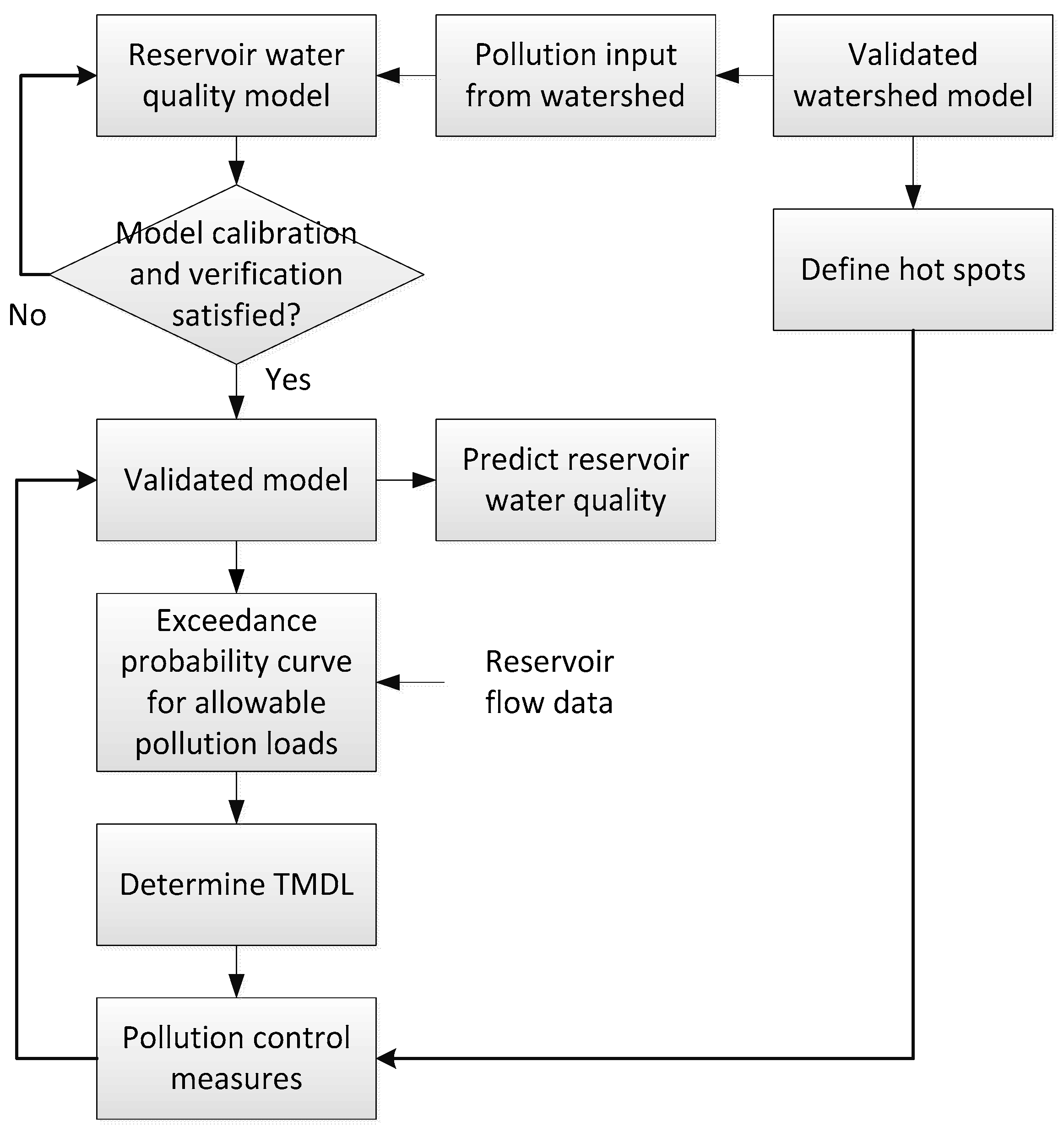
This study focused on reservoir TMDL and required a reservoir water quality model and a watershed model. A flowchart of this study is shown in Figure 1. The watershed model was used to model the nonpoint source pollution and the transportation of pollutants across the watershed. The reservoir water quality model was used to predict water quality changes in reservoirs. The pollutants generated from the watershed became the inputs of the reservoir water quality model. Before combining the two models, model calibration and the validation of the watershed model were conducted. When the quality of the pollutant input was acceptable, model calibration and validation of the reservoir model were implemented sequentially. The validated reservoir model illustrates the relationship between pollutant inputs from the watershed and the water quality changes in the reservoir. It was used to determine the allowable pollutant loadings under a required water quality standard. The main contribution of this study is that an exceedance probability curve of the allowable pollution loads under fixed and ideal water quality concentrations in a reservoir is suggested as a TMDL value. In addition, the validated watershed model can demonstrate the spatial distributions of pollutants and identify pollution hot spots, which can inform the design of pollution control measures based on the determined TMDL value. The reservoir and watershed models in the study flowchart are not the only models possible when using this approach. Users can select models according to their preferences and the available data to ensure that the results of the model are reliable.

2.2. Reservoir Model: Vollenweider Model

The reservoir water quality model used in this study is the Vollenweider model [15,16], which has been used widely to assess phosphorous (P) concentrations in lakes and reservoirs. The Vollenweider model is a one-dimensional mass-balance model that assumes that the change in the P concentration over time is equal to the input P concentration minus the output P concentration and the amount of P lost inside the waterbody. Based on this assumption, the P is completely mixed in the reservoir and the output P concentration is the same as the P concentration in the reservoir. In addition, P is lost when it settles in the sediment. The Vollenweider equation is as follows.
Δ P V Δ t = M ( P × Q ) ( P V × σ )
where PV = total mass of P in reservoir (g); P = P concentration (g/m3); V = reservoir water volume (m3); t = time; M = annual mass of P input (g/year); Q = annual volume of water outflow (m3/year); σ = settling coefficient (year−1).
The main problem encountered when using the Vollenweider model is that the settling coefficient is difficult to measure in different waterbodies. One of the most common solutions was developed by Kirchner and Dillon [17], who suggested that the proportion of P lost to sediment (Rp) can be estimated as R p = v / ( v + q s ) , where v is the settling velocity (m/year) and qs is the areal hydraulic load (m/year). The parameter qs is calculated from the total flow entering the reservoir (m3/year) divided by the surface area of the reservoir (m2). When incorporating this equation into the Vollenweider equation under the steady-state assumption, Equation (1) can be transformed to Equations (2) and (3).
Δ P V Δ t = M ( P × Q ) ( M × R p ) = 0
P = M ( 1 R p ) Q
In Equation (3), the P concentration is calculated based on the input P loads (M), outflow discharge (Q), and lost proportion (Rp). Rp is obtained by considering the settling velocity (v) and the actual inflow and reservoir surface area (A) data. In this study, M was generated from a validated watershed model. Inflow and outflow data and water surface area were obtained from official monitoring stations. Under ideal conditions, as the water volume changes, the water surface area also changes. However, we did not have precise surface area data for calculating qs, which is used to calculate Rp. Instead, a maximum water surface area was used. Using a fixed A affects the accuracy of qs, but its influence might be less than the influences of M and Q in the final TP concentration equation. This is a limitation of field-obtained data and is one factor affecting the precision of model simulation. The only unknown parameter was settling velocity (v). The parameter is adjusted and determined via model calibration and validation. Once we verified the settling velocity, the allowable M for a target P concentration was generated considering different inflow and outflow conditions. Finally, we obtained a curve of the allowable M for a target P concentration and determined the distribution of the curve using the exceedance probability.

2.3. Watershed Model: SWMM Model

M can be obtained using several methods, such as the simple export coefficient method or via a complex watershed model. In this study, the SWMM (Storm Water Management Model) was used because the monitored climate, flow, and water quality data were sufficient and because this model has been successfully applied in several cases in Taiwan [18,19]. In addition, the SWMM model includes an LID (low impact development) module, and it can assess the performance of different structural best management practice (BMP) facilities. The SWMM model was established by the U.S. Environmental Protection Agency (USEPA) and is freely available for downloading from their website. Before running the SWMM model, the GIS layers, including the watershed boundary, land use, digital elevation model (DEM), and river layers, are required. These GIS data are uploaded and combined using the BASINS (Better Assessment Science Integrating Point and Nonpoint Sources) platform to generate the necessary properties of the watershed for the SWMM model calculations. While the characteristics of the watershed are prepared, the rainfall data are inputted to simulate the hydrological performance. Model parameters or coefficients are determined by local references or through a calibration and validation process.
In the SWMM model, subwatersheds are hydrologic units of land in which the topography and drainage system elements direct surface runoff to a single discharge point. Each subwatershed is divided into pervious and impervious areas. The percentages of pervious and impervious area of the subwatershed are decided by the land use. Surface runoff can infiltrate the pervious subarea but not the impervious subarea. In the calculation of surface runoff, each subwatershed surface is treated as a nonlinear reservoir. Surface runoff occurs when the depth of water in the subwatershed exceeds the maximum depression storage, in which case the outflow is calculated by Manning’s equation. Therefore, Manning’s n for overland flow for both pervious and impervious areas is required. SWMM offers three infiltration methods: Horton infiltration, Green–Ampt infiltration, and Curve Number infiltration. In the present case study, we selected the Horton infiltration method. If users consider the effects of snow and groundwater, the snow-pack object and groundwater parameters need to be assigned. In this study, we did not include these two objects.
In the SWMM model, nonpoint source pollution is calculated from buildup and wash-off functions. The two functions calculate how many pollutants accumulate on dry days and wash away on wet days. Different functions are used for different land-use types, and the coefficients of the functions are confirmed through model validation. The detailed partitions in different phases and the transportation of pollutants are not included in this model. A more precise watershed model, GSSHA (Gridded Surface Subsurface Hydrologic Analysis), is suggested if more data are available [20].
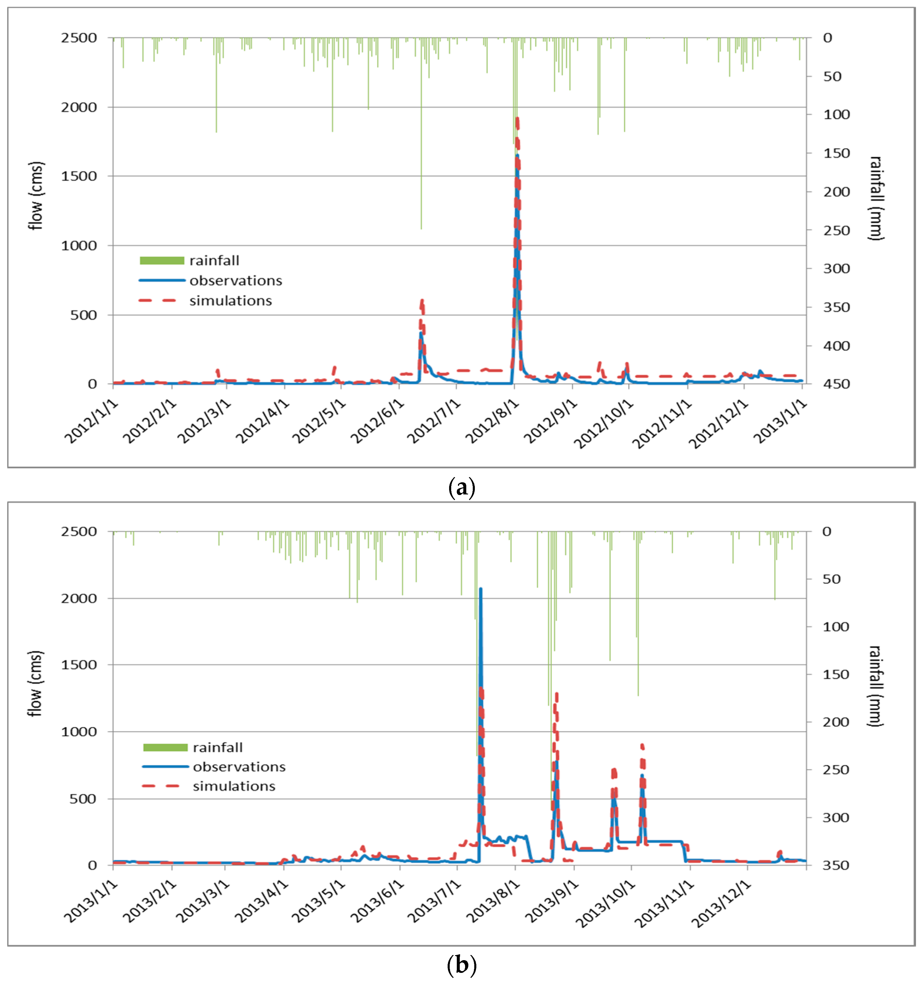
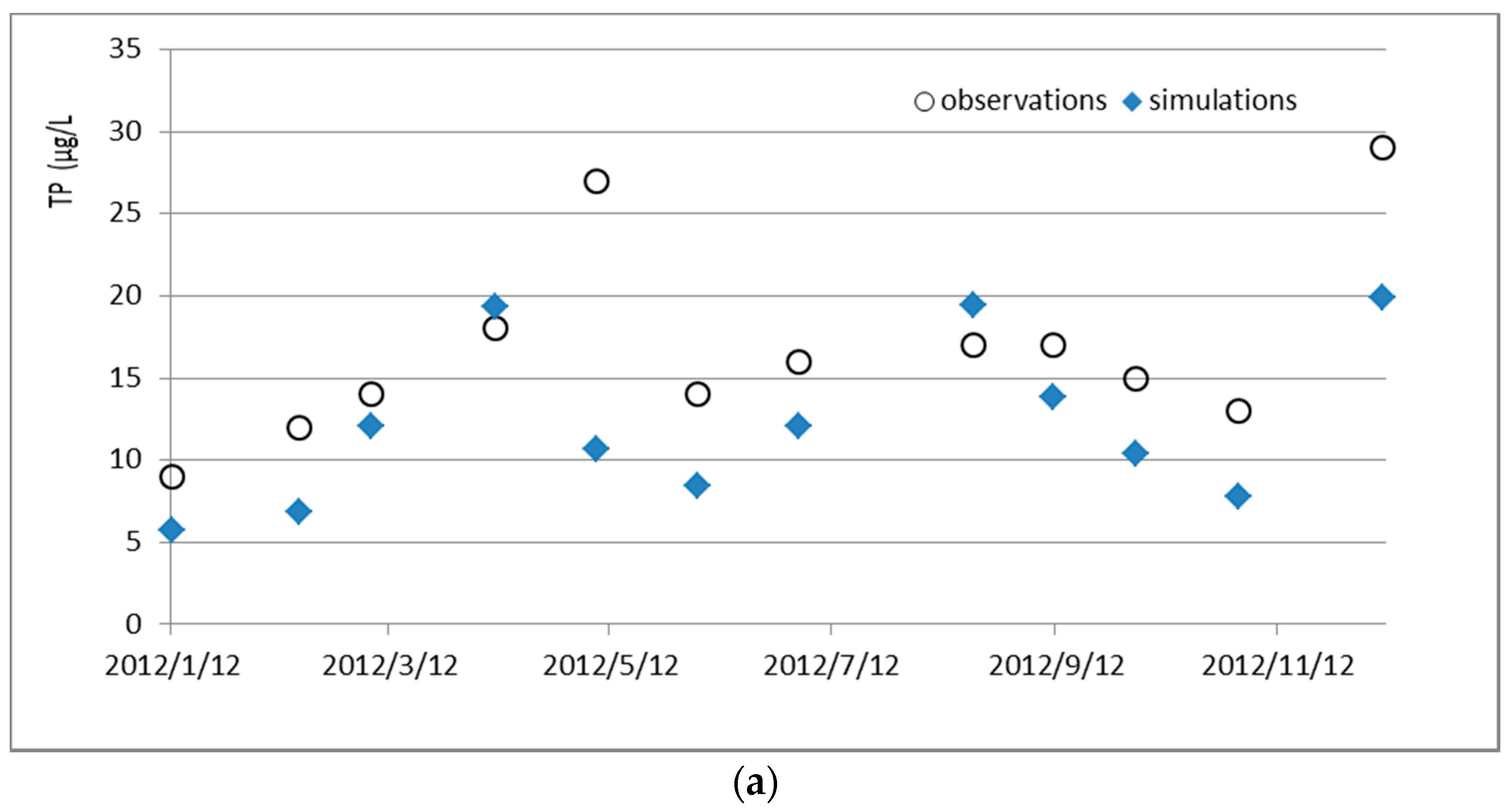
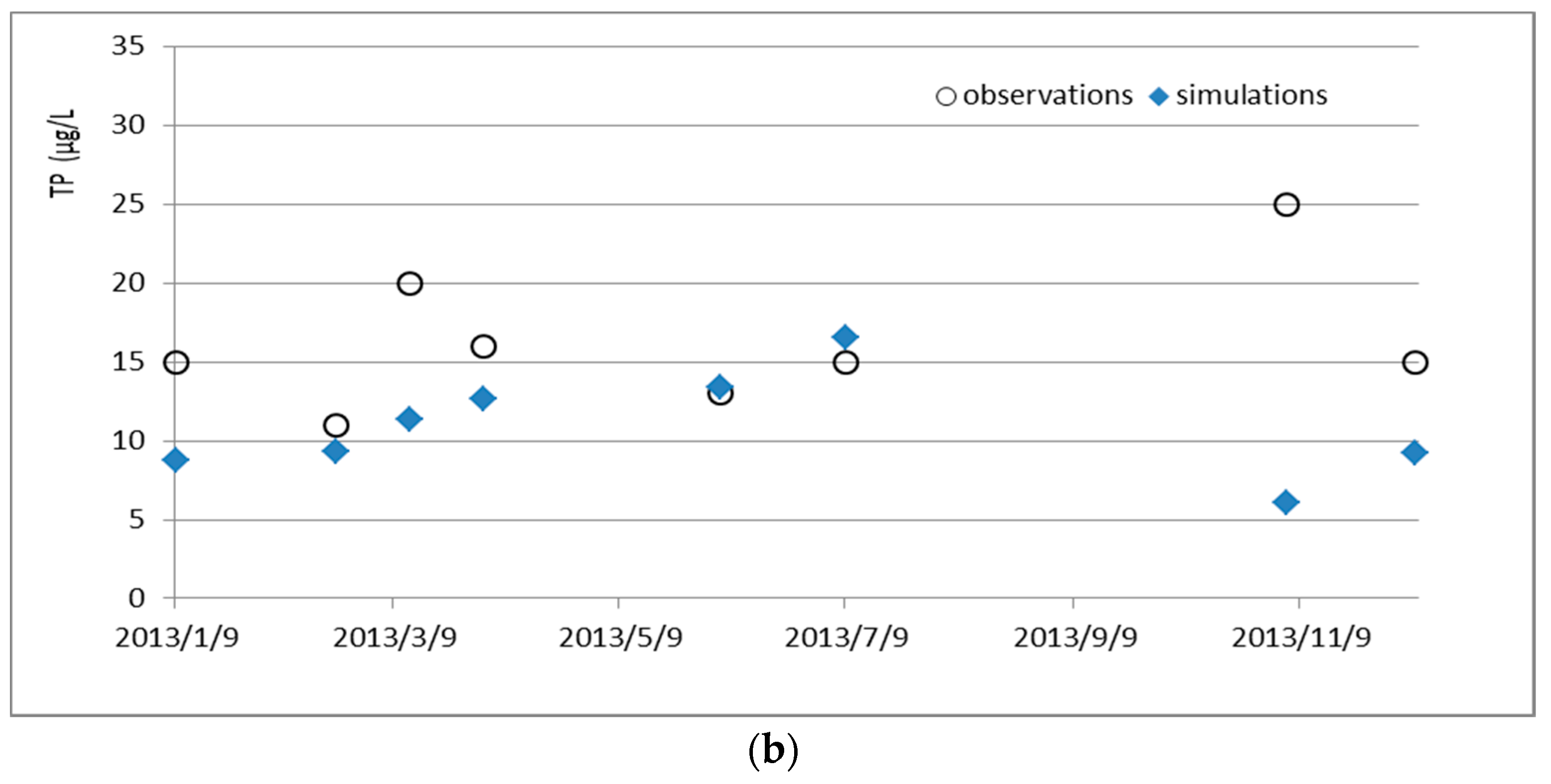
The SWMM model should be calibrated and validated to ensure its reliability before it is used to obtain input P loads for the Vollenweider model. Realistic flow and water quality data obtained from monitoring stations were collected to compare with the simulated data at the same locations. Several statistical analyses can be used, such as r (Pearson’s correlation coefficient), R2 (coefficient of determination), MAPE (mean absolute percentage error), and NSE (Nash–Sutcliffe efficiency) [21]. We used R2 and MAPE, which are commonly used in Taiwan, to determine the fitness of the model. Various model parameters need to be adjusted, and the parameters for flow and water quality are different. It is helpful to begin by considering the most sensitive model parameters. The most sensitive model parameters of the SWMM model are described by Chen et al. [19]. When the final model parameters are determined by model calibration and validation, the parameter values only fit the observed data. Although more observations might be helpful to obtain more realistic parameter values, in the present case, the parameter values introduce unavoidable uncertainty. Based on the results of model evaluation, we can adopt sufficiently accurate simulations, resulting in an acceptable level of model uncertainty. The unacceptable uncertainty should not be applied for decision-making.

3. Study Area

The Shiman Reservoir was constructed in 1964 and has a total water storage volume of 201.24 million m3, a water surface area of approximately 8 km2 and a watershed area of 736.4 km
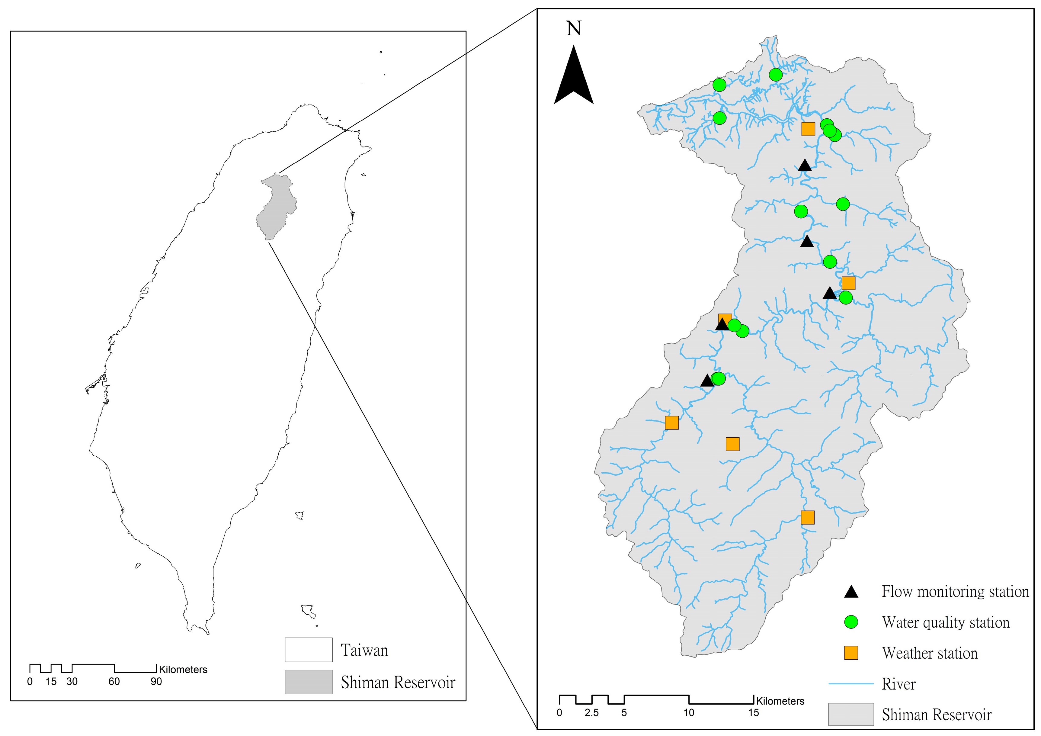
2. The Shiman Reservoir is a multiple-function reservoir that is used for drinking water, irrigation, electricity generation, flood control, and recreation. The reservoir provides drinking water for nearly 2 million people in Taoyuan City, Taiwan. It is located upstream of Dahan Creek in northern Taiwan (Figure 2). The elevation of the watershed ranges from 100 m to 3500 m; accordingly, the flow rate is high, and serious soil erosion occurs. In this reservoir, several efforts have been made to mitigate soil erosion and reduce the amount of sediment entering the reservoir. Previous reservoir management measures satisfactorily reduced the sediment in the reservoir. However, although the turbidity of the water was decreased, eutrophication continued to occur.
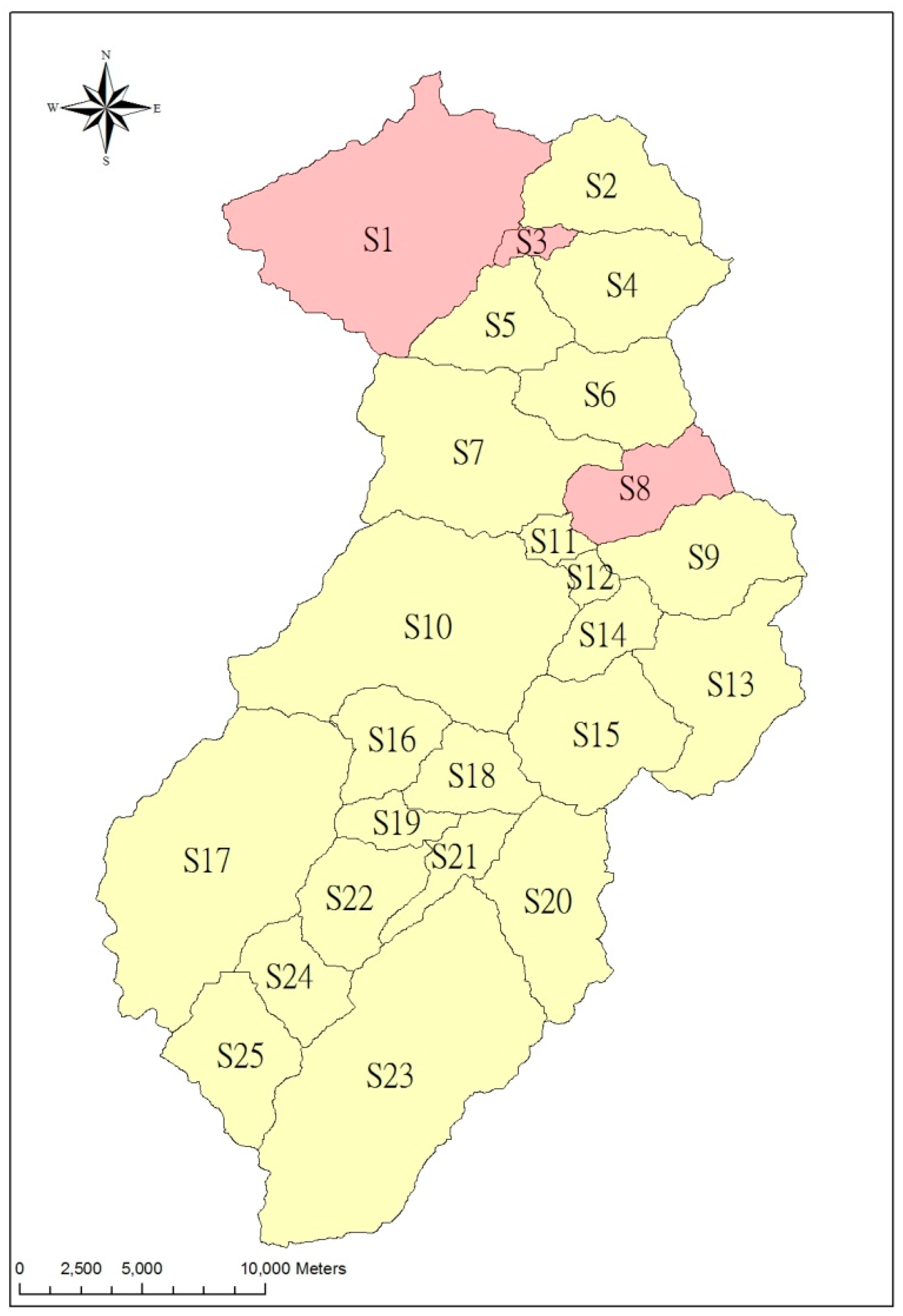
The monitoring stations in the watershed of the reservoir include 6 weather stations, 5 flow monitoring stations, and 13 water quality monitoring stations. The locations of these stations are shown in 
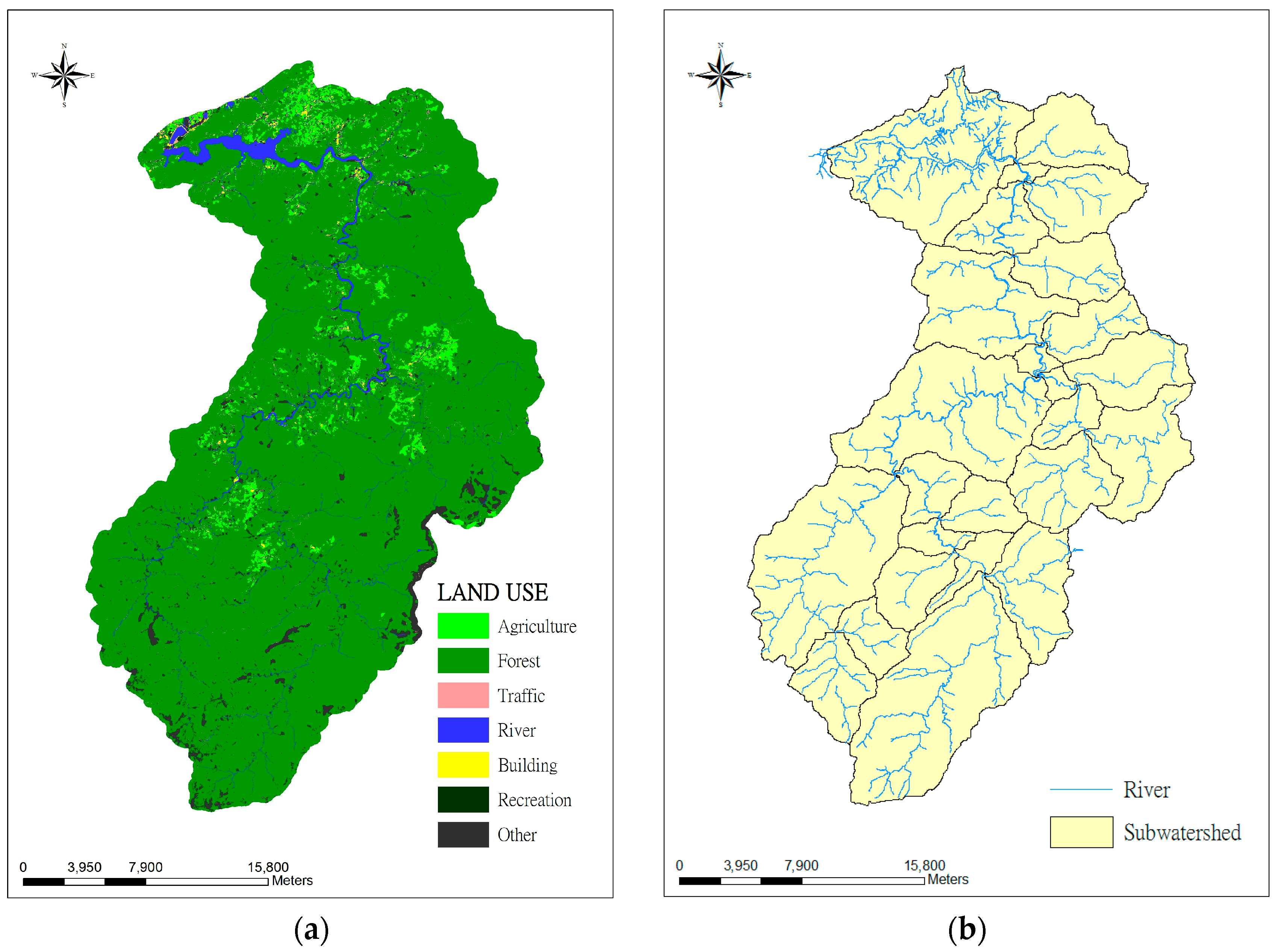
Figure 2. Rainfall data are required to apply a watershed model. Thus, the rainfall data from the 6 stations were merged using the Thiessen polygon method, in which the contributing area is divided and used as a weighting factor. The land-use and river distribution of the watershed is shown in Figure 3. The land use of the Shiman Reservoir watershed is 78.3% forest and 14.8% agricultural land. Only 0.4% of the total land area is used for residential use. The potential pollution sources are nonpoint source pollution from agricultural lands and point-source pollution from untreated domestic sewers. The increasing tourist population is also a threat to water quality because the sewage system is not distributed throughout the entire watershed.
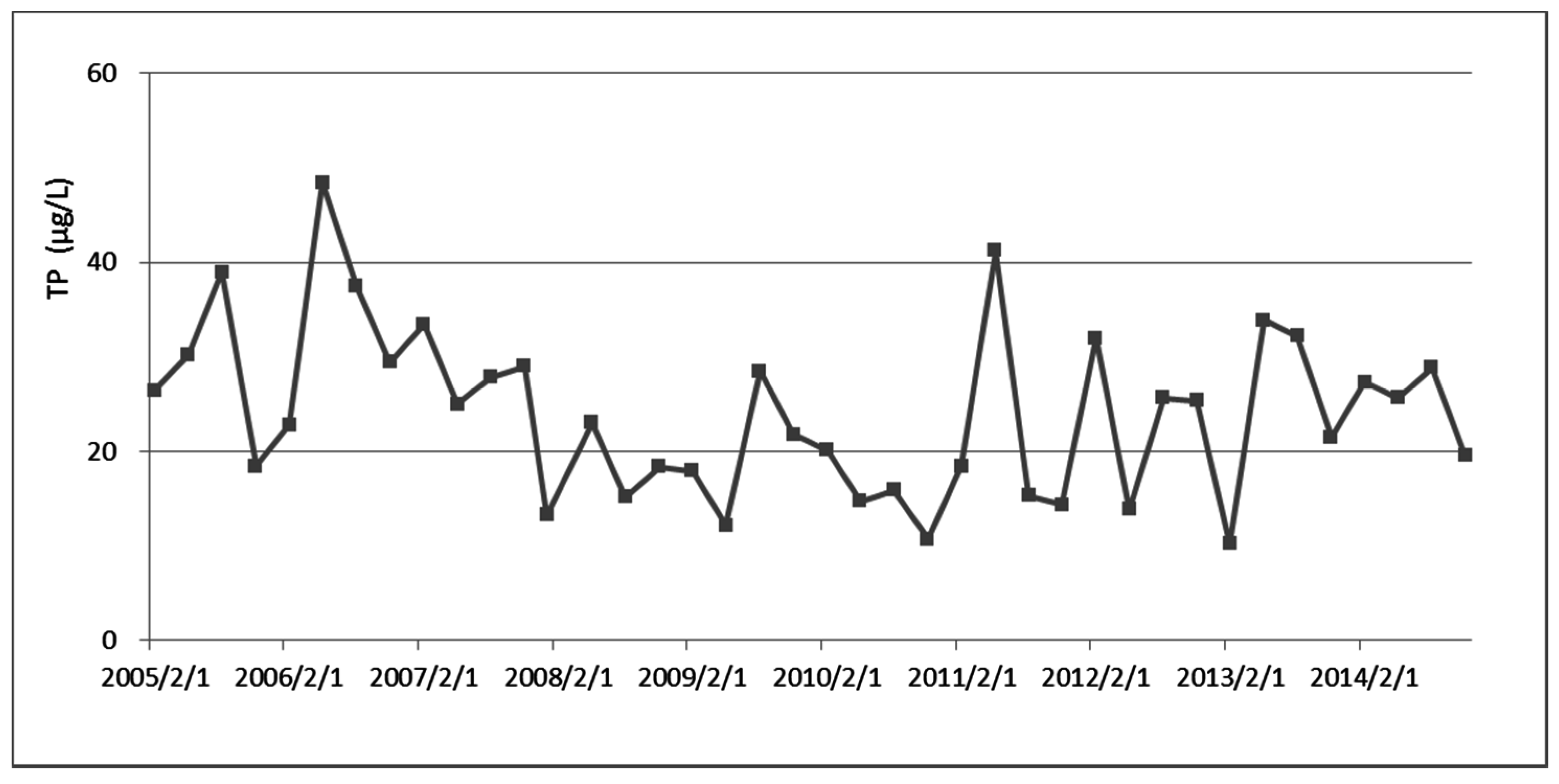
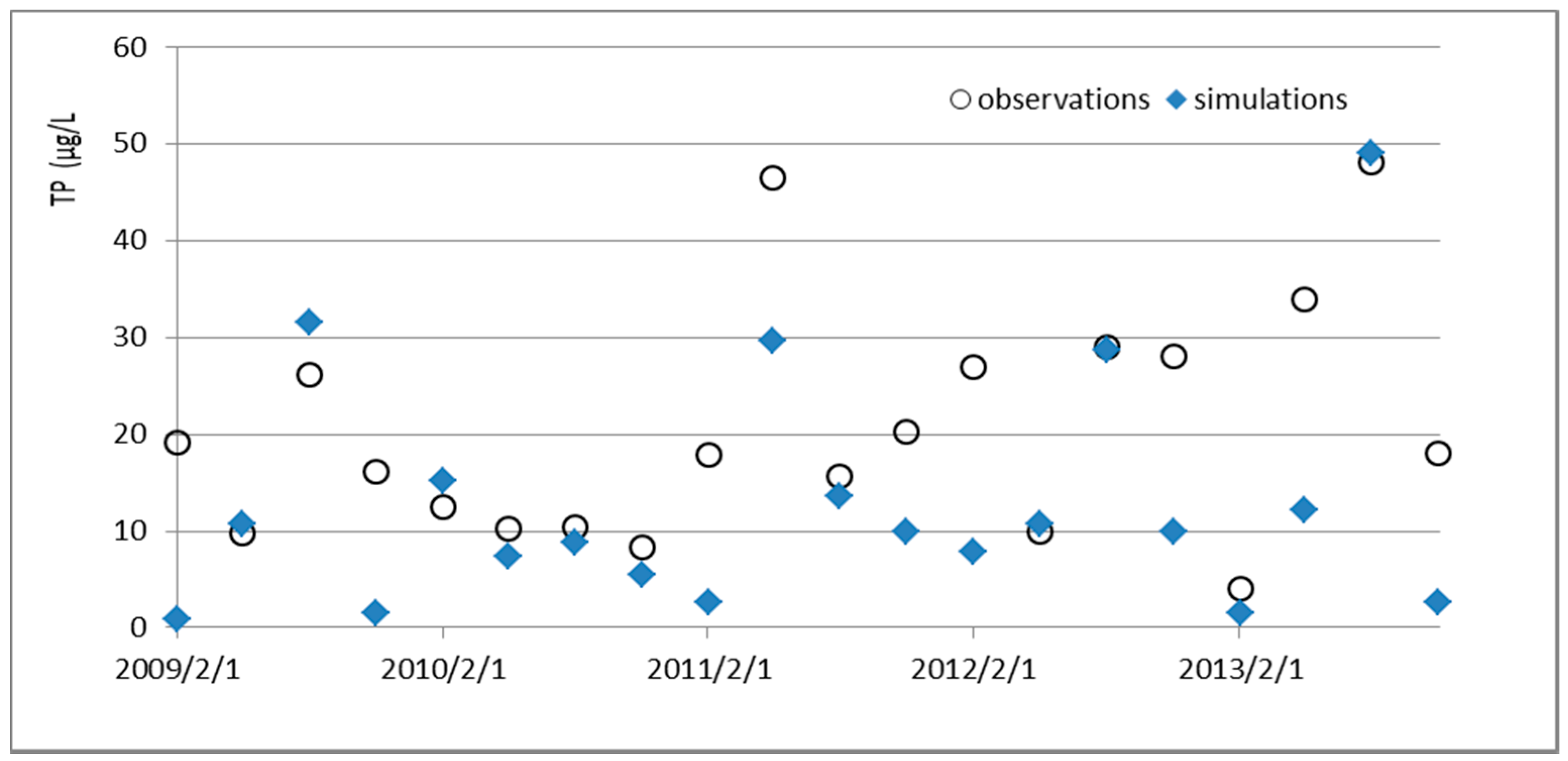
The average total nitrogen (TN)/TP ratio in the reservoir is 13.67, which indicates that TP is the most restricting factor in the reservoir. Thus, to control eutrophication, the TP input should be reduced. The standard TP concentration of the Shiman Reservoir is 20 μg/L. However, in the last 10 years, the maximum TP concentration reached as high as 48.4 μg/L, and the average TP concentration was 25.0 μg/L (Figure 4).

4. Results and Discussion

4.1. Watershed Model Calibration and Validation Results

The observed flow data consisted of continuous daily data, and the observed water quality consisted of monthly data. The water quality was sampled and analyzed once a month, yielding a total of 12 observed data sample sets in each year. The data from 2012 were used for model calibration to identify adequate model parameters, and the data from 2013 were used for model verification to verify the feasibility of the model parameters. Figure 5 presents the results of the flow simulation, and Figure 6 presents the results of the TP simulation.
In the model simulation process, flow is simulated before water quality. The R2 values obtained from the calibration and verification tests were 0.83 and 0.64, respectively. After the simulation of flow was deemed acceptable, the water quality simulation was implemented, and the model parameters for simulating flow no longer changed during the water quality simulation. The MAPEs for the TP simulation were 30.0% for calibration and 31.0% for validation. Although the MAPE values were considered acceptable, the R2 values for TP simulation were low: 0.38 for calibration and 0.18 for validation. However, the R2 value is focused on the correlation. Because the water quality data are not continuous like the flow data, the R2 value might not be appropriate for representing the simulation acceptance of water quality. The MAPE results indicate that the difference between simulations and observations is less than 50%, which is regarded as an acceptable percentage. Some important model parameters were validated and are summarized in Table 1.

4.2. Reservoir Model Calibration and Validation Results

In the Vollenweider model, all equation parameters are denoted from realistic data except for the settling velocity (v), which differs among different reservoirs, and no experimental value for the Shiman Reservoir was obtained. Therefore, this parameter must be verified before it is applied. Observed TP concentrations were compared with the simulated TP concentrations to determine the appropriate v value. The input TP mass was obtained using verified SWMM. The input data used in the Vollenweider model are summarized in Table 2. The TP concentration in the reservoir was sampled each season for a total of four observations per year. Therefore, we used 5-year data to calibrate and verify the model (Figure 7). Consequently, the verified settling velocity for the Shiman Reservoir was 10 m/year.

4.3. Determination of Maximum Allowable Daily Loads of TP

The main objective of this study was to determine the maximum allowable daily load of TP for reservoirs. When the target TP concentration is determined, the total TP input mass is determined from the input and outflow of the reservoir using the previously verified reservoir model. Thus, when we input realistic discharge values for the reservoir into the model, the allowable TP input mass that meets the target TP concentration is produced.
The required P concentration is 20 μg/L for the Shiman Reservoir. The allowable TP input mass at the fixed TP concentration of 20 μg/L is obtained using the previous 5 years of flow data, and its accumulative probability distribution is shown in Figure 8. In addition to the TP of 20 μg/L, a TP concentration of 24 μg/L is shown in the figure because a TP concentration greater than 24 μg/L is recognized as a eutrophic state based on the CTSI (Carlson Trophic State Index), which is officially used to represent eutrophication states in Taiwan. The allowable TP input mass at the exceedance probability of 50% means that the input mass could protect the reservoir by avoiding the TP concentration target at the probability level of 50%; we call this input mass M50. Therefore, M75 indicates that there is a 75% probability that this input mass could protect the reservoir and prevent TP concentrations greater than the target value. M90 provides a higher level of protection because the allowable input mass is more limited. The allowable TP input masses for different exceedance probabilities are listed in Table 3. We suggest that M50 can be used as the TMDL of the reservoir as a short-term strategy and that M75 or M90 can be used as a long-term strategy. The particular exceedance probability applied in any given case will depend on policy decision-making. For the Shiman Reservoir, the proposed allowable TP input mass is 22,209 kg/year (M50).
A simple average water volume should not be used to determine the reservoir TMDL because the water volume is controlled by manual operation and is not normally distributed (see Figure 8). For the Shiman Reservoir, considering an average water volume could indicate that the allowable pollution load is approximately 70,000 kg/year. This load would meet the TP standard at the 10% probability level, with the reservoir experiencing pollution or eutrophication >90% of the time. When considering the actual hydraulic conditions, the exceedance probability would provide feasible and objective information for determining the assimilative capacity of a reservoir.

4.4. Pollution Control Strategies and Their Performances for Improving Reservoir Water Quality

When determining the allowable TP input mass, the following procedure was used to allocate the input mass into the watershed and decrease the pollution content of the reservoir. Because it is a large watershed, the pollution hot spots in the reservoir are first defined as priority pollution control areas. The three following principles are used for defining these hot spots: the total contributed pollution loads, the percentages of point pollution sources, and the pollution load per land area. Of the 25 subwatersheds considered in this study, three subwatersheds were ranked as hot spots (Figure 9). The subwatersheds S1, S3, and S8 were characterized as areas of high pollution potential because they have high total pollution loads, a high percentage of point pollution sources, and high pollution loads per land area. At this stage, the subwatersheds with high potential pollution were identified. When detailing the sites and locations for best management practices (BMPs) and when determining load allocation, the advanced spatial optimization model might be needed, which includes cost-effectiveness and uncertainty considerations [22,23].
The current average TP concentration in the studied reservoir is 25 μg/L, and the current average TP input mass is 32,475 kg/year. If the target allowable TP input mass is 22,209 kg/year (M50), pollution should be reduced by 31.6%. Because the locations of the pollution hot spots have been defined, the required pollution reduction can be implemented in these areas first. The potential reduction of TP from point sources in the three hot spots is 1018 kg/year, and the potential reduction of TP from nonpoint sources is 2694 kg/year. The reduction of TP from point pollution sources could be achieved by improving domestic wastewater treatment. The reduction of TP from nonpoint sources could be achieved by using various BMPs, including structural and nonstructural measures. Therefore, controlling pollution at the three hot spots could decrease the TP from its current value of 25 μg/L to 22 μg/L. The TMDL and predicted TP concentration are shown in Figure 10. The control of hot spots can be regarded as a short-term management goal. If the goal of 20 μg/L is to be reached, pollution control measures must be implemented in the remaining subwatersheds.

5. Conclusions

Determining the allowable load of a waterbody is important for implementing TMDLs and affects the subsequent pollution control practices. However, it is difficult to determine the flow status in a reservoir because the inflow and outflow are not equal. In this study, we used the exceedance probability to demonstrate the relationships between water quality and allowable loads. The results of this study imply that allowable loads can be met (without exceeding the target water quality concentration). The concept of this study is simple and can be applied to any lake or reservoir. In this study, we suggest using M50, which represents an exceedance probability of 50%. For stricter limitations, M75 or M90 can be considered. Notably, using the average reservoir volume significantly overestimates the assimilative ability and might fail to protect the reservoir. The manual operation of the reservoir water level affects the water volume and TP concentration. Thus, we suggest that the average reservoir water volume should not be used to determine the allowable loads.
To determine the allowable loads, it is necessary to combine the watershed and reservoir models. The choice of model is not limited to the two models used in this study. We chose the SWMM and Vollenweider models because they have been successfully applied in other cases in Taiwan. Users of this approach can follow the flowchart in this study and select the appropriate models for their case studies. In this study, we provide a total pollution reduction and do not show the water improvement performance of each pollution control practice, such as different BMPs. If no feasible watershed model exists, the exceedance probability method can be used to determine the maximum allowable load of a reservoir by replacing the watershed results with actual observations of inflow pollution loads.

Acknowledgments

The authors would like to thank the Environmental Protection Administration of the Republic of China (Taiwan) for financial supports.

Author Contributions

All authors were involved in designing and discussing the study. Chi-Feng Chen drafted and finalized the manuscript. Lin-Yi Tsai and Chi-Hsuan Fan collected the necessary data and executed the model. Jen-Yang Lin coordinated the group and revised the manuscript. All authors have read and approved the final manuscript.

Conflicts of Interest

The authors declare no conflict of interest.

References

  1. United States Environmental Protection Agency (USEPA). Protocol for Developing Pathogen TMDLs; EPA 841-R-00-002; Office of Water (4503F): Washington, DC, USA, 2001.
  2. National Research Council (NRC). Assessing the TMDL Approach to Water Quality Management; Committee to Assess the Scientific Basis of the Total Maximum Daily Load Approach to Water Pollution Reduction; Water Science and Technology Board: Washington, DC, USA, 2001. [Google Scholar]
  3. Boyacioglu, H.; Alpaslan, M.N. Total maximum daily load (TMDL) based sustainable basin growth and management strategy. Environ. Monit. Assess. 2008, 146, 411–421. [Google Scholar] [CrossRef] [PubMed]
  4. Elshorbagy, A.; Teegavarapu, R.S.V.; Ormsbee, L. Total maximum daily load (TMDL) approach to surface water quality management: Concepts, issues, and applications. Can. J. Civ. Eng. 2005, 32, 442–448. [Google Scholar] [CrossRef]
  5. Kang, M.S.; Park, S.W.; Lee, J.J.; Yoo, K.H. Applying SWAT for TMDL programs to a small watershed containing rice paddy fields. Agric. Water Manag. 2006, 79, 72–92. [Google Scholar] [CrossRef]
  6. Wang, C.; Bi, J.; Ambrose, R.B. Development and application of mathematical models to support total maximum daily load for the Taihu Lake’s influent rivers, China. Ecol. Eng. 2015, 83, 258–267. [Google Scholar] [CrossRef]
  7. Borah, D.K.; Yagow, G.; Saleh, A.; Barnes, P.L.; Rosenthal, W.; Krug, E.C.; Hauck, L.M. Sediment and nutrient modeling for TMDL development implementation. Trans. ASABE 2006, 49, 967–986. [Google Scholar] [CrossRef]
  8. DePinto, J.V.; Freedman, P.L.; Dilks, D.M.; Larson, W.M. Models quantify the total maximum daily load process. J. Environ. Eng. 2004, 130, 703–713. [Google Scholar] [CrossRef]
  9. United States Environmental Protection Agency (USEPA). Options for Expressing Daily Loads in TMDLs; Office of Wetlands, Oceans & Watersheds: Washington, DC, USA, 2007.
  10. Mishra, P.K.; Deng, Z.Q. Sediment TMDL development for the Amite River. Water Resour. Manag. 2009, 23, 839–852. [Google Scholar] [CrossRef]
  11. Gaddis, E.J.B.; Voinov, A. Spatially explicit modeling of land use specific phosphorus transport pathways to improve TMDL load estimates and implementation planning. Water Resour. Manag. 2010, 24, 1621–1644. [Google Scholar] [CrossRef]
  12. Gulati, S.; Stubblefield, A.A.; Hanlon, J.S.; Spier, C.L.; Stringfellow, W.T. Use of continuous and grab sample data for calculating total maximum daily load (TMDL) in agricultural watersheds. Chemosphere 2014, 99, 81–88. [Google Scholar] [CrossRef] [PubMed]
  13. Steinman, A.D.; Ogdahl, M.E. TMDL reevaluation: Reconciling internal phosphorus load reductions in a eutrophic lake. Lake Reserv. Manag. 2015, 31, 115–126. [Google Scholar] [CrossRef]
  14. Havens, K.E.; Walker, W.W. Development of a total phosphorus concentration goal in the TMDL process for Lake Okeechobee, Florida (USA). Lake Reserv. Manag. 2002, 18, 227–238. [Google Scholar] [CrossRef]
  15. Vollenweider, R. Scientific Fundamentals of the Eutrophication of Lakes and Flowing Waters, with Particular Reference to Nitrogen and Phosphorus as Factors in Eutrophication; DAS/CSI/68.27; Organisation for Economic Co-Operation and Development (OECD): Paris, France, 1968. [Google Scholar]
  16. Vollenweider, R. Input-Output models with special reference to the phosphorus loading concept in limnology. Schweiz. Z. Hydrol. 1975, 37, 53–83. [Google Scholar]
  17. Kirchner, W.B.; Dillon, P.J. An empirical method of estimating the retention of phosphorus in lakes. Water Resour. Res. 1975, 11, 182–183. [Google Scholar] [CrossRef]
  18. Wang, C.W.; Chen, C.F.; Lin, J.Y. Effects of buffer strips on reducing nonpoint source pollution and improving water quality in Feitsui Reservoir. J. Chin. Soil Water Conserv. 2014, 45, 207–215. [Google Scholar]
  19. Chen, C.F.; Sheng, M.Y.; Chang, C.L.; Kang, S.F.; Lin, J.Y. Application of the SUSTAIN model to a watershed-scale case for water quality management. Water 2014, 6, 3575–3589. [Google Scholar] [CrossRef]
  20. Pradhan, N.R.; Downer, C.W.; Johnson, B.E. A Physics Based Hydrologic Modeling Approach to Simulate Non-point Source Pollution for the Purposes of Calculating TMDLs and Designing Abatement Measures. In Practical Aspects of Computational Chemistry III; Springer: New York, NY, USA, 2014; pp. 249–282. [Google Scholar]
  21. Moriasi, D.N.; Arnold, J.G.; Van Liew, M.W.; Bingner, R.L.; Harmel, R.D.; Veith, T.L. Model evaluation guidelines for systematic quantification of accuracy in watershed simulations. Trans. ASABE 2007, 50, 885–900. [Google Scholar] [CrossRef]
  22. Yang, G.; Best, E.P.H. Spatial optimization of watershed management practices for nitrogen load reduction using a modeling-optimization framework. J. Environ. Manag. 2015, 161, 252–260. [Google Scholar] [CrossRef] [PubMed]
  23. Zhou, F.; Dong, Y.; Wu, J.; Zheng, J.; Zhao, Y. An indirect simulation-optimization model for determining optimal TMDL allocation under uncertainty. Water 2015, 7, 6634–6650. [Google Scholar] [CrossRef]
Figure 1. Flowchart showing how the exceedance probability curve was produced for reservoir total maximum daily loads (TMDLs).
Water 08 00541 g001
Figure 2. The location of the Shiman Reservoir and the locations of the monitoring stations within the reservoir.
Water 08 00541 g002
Figure 3. The land use and rivers in the Shiman Reservoir watershed. The watershed was divided into 25 subwatersheds, which were used in the watershed model simulations. (a) The distribution of land use in the watershed; and (b) the results of watershed delineation.
Water 08 00541 g003
Figure 4. Total phosphorous (TP) concentrations in the Shiman Reservoir in 2005–2015. The standard TP concentration is 20 μg/L.
Water 08 00541 g004
Figure 5. The flow simulation results. (a) The model calibration using the 2012 data; (b) the model validation using the 2013 data.
Water 08 00541 g005
Figure 6. The TP simulation results. (a) The model calibration using the 2012 data, and (b) the model validation using the 2013 data.
Water 08 00541 g006aWater 08 00541 g006b
Figure 7. Validation of the Vollenweider model.
Water 08 00541 g007
Figure 8. The exceedance probability of the input TP loads. This probability is regarded as the protection level to ensure that the reservoir TP concentration remains below the target concentration under certain input loadings.
Water 08 00541 g008
Figure 9. The hot spots (the areas with the highest pollution potential) of the Shiman Reservoir subwatersheds: S1, S3, and S8.
Water 08 00541 g009
Figure 10. The predicted TMDL performance of the Shiman Reservoir and the relationships of the watershed TP loads and reservoir TP concentrations. For example, controlling the point source (PS) pollution in hot spots could reduce the TP load by 1018 kg/year and reduce the TP concentration from 25 to 24 μg/L. Subsequent control of nonpoint source (NPS) pollution in the hot spots could reduce the TP load by 2694 kg/year and result in a TP concentration of TP 22 μg/L. The target TP concentration is 20 μg/L, and the maximum allowable load is 22,209 kg/year.
Water 08 00541 g010
Table 1. Important SWMM (Storm Water Management Model) parameters used in this study.
ObjectParametersValidated ValueRange
Surface runoffManning’s n for pervious areas0.20.1–0.8
Manning’s n for impervious areas0.030.01–0.05
Infiltration (Horton infiltration)Max Infiltration (mm/h)2.70.25–25
Min Infiltration (mm/h)2.40.25–25
Decay Constant (1/h)40—none
Pollutant (TP)
Buildup (Power Function)Max. Buildup (kg)Agriculture: 395
Forest: 22
Urban: 288.5
Camp site: 22
Barren land: 140
0—none
Rate Constant (1/day/area)All land use: 10—none
Power ConstantAll land use: 0.50—none
Wash off (Event Mean Concentration)Wash-off exponentAll land use: 10—none
Wash-off pollutant concentration (mg/L)Agriculture: 270
Forest: 20
Urban: 228.5
Camp site: 20
Barren land: 111
0—none
Table 2. The input data and their sources for the Vollenweider model applied to the Shiman Reservoir, Taiwan.
ParametersDefinitionsValues/Sources
QinInflow discharge (m3/year)Actual monitoring data
QoutOutflow discharge (m3/year)Actual monitoring data
AReservoir surface area (m2)8,000,000
RpLoss percentage of P in the reservoirCalculated from v/(v + qs)
qsAreal hydraulic load (m/year)Calculated from Qin/A
MTotal TP input mass (g/year)Obtained from the verified SWMM
PTP concentration in the reservoir (g/m3)Calculation results from the Vollenweider model
vSettling velocity of P (m/year)10 (after model verification)
Table 3. The allowable TP input mass for exceedance probabilities of 25%, 50%, 75%, and 90% at the target TP concentrations of 20 μg/L and 24 μg/L.
Exceedance ProbabilitySymbolTP = 20 μg/LTP = 24 μg/L
Allowable TP Input Mass (kg/Year)Allowable TP Input Mass (kg/Year)
25%M2528,36334,036
50%M5022,20926,651
75%M7516,77620,131
90%M9013,03915,647

