Article

Effect of the Resolution of Tipping-Bucket Rain Gauge and Calculation Method on Rainfall Intensities in an Andean Mountain Gradient

1
Departamento de Recursos Hídricos y Ciencias Ambientales, Universidad de Cuenca, Cuenca 010150, Ecuador
2
Facultad de Ciencias Agropecuarias, Universidad de Cuenca, Cuenca 010150, Ecuador
*
Author to whom correspondence should be addressed.
Water 2016, 8(11), 534; https://doi.org/10.3390/w8110534
Submission received: 30 August 2016 / Revised: 26 October 2016 / Accepted: 2 November 2016 / Published: 16 November 2016

Abstract

:
A laser-optical disdrometer served as reference to assess the absolute percent bias of calculated rainfall intensity using the data of different-resolution tipping-bucket rain gauges classically applied by climatologists and hydrologists in the Andean region. Additionally, the impact of the calculation method (tip counting versus cubic spline interpolation) was examined. The combined effect was assessed for different rainfall intensity classes (0–0.99, 1–1.99, 2–4.99, and 5–10 mm·h−1) and timescales (5, 10, 30, and 60 min). Additionally, the variation in percent absolute bias of the Davis rain gauge, the collector most widely used in the study region, was defined with respect to the Texas rain gauge along an elevation gradient between 3300 and 4000 m a.s.l. Results reveal that the value of the percent absolute bias is largest for small rainfall intensities (≤2 mm·h−1) and short timescales (≤10 min), and decreases when the cubic spline interpolation is used. No relation was found between the error, the elevation, and rainfall depth along the gradient. Based on the research findings, it is recommended to measure precipitation in the high Andean mountain region with a high-resolution sensor and to consider cubic spline for the computation of intensities.

1. Introduction

Precipitation is a major component of the water cycle and is responsible for the deposition of fresh water on Earth—it provides the water for domestic, agricultural, and industrial uses, as well as aquatic and non-aquatic ecosystems, and its measurement is considered a most important task in hydrology [1]. Specifically, in the páramo eco-region of the northern Andes, a correct measurement of precipitation is essential given the economic, ecological, and social function of this ecosystem for the surrounding societies, and the overall fragility of the ecosystem. The páramo consists of a collection of neo-tropical alpine grasslands [2], covering an area in the northern Andes of 35,000 km2 [3] that is situated between 3000 and 4800 m above sea level (m a.s.l.) [4].
The water regulating function of the páramo is increasingly amended by natural and human processes (global environmental change) [2,5,6,7], and requires correct conservation, management, and accurate measurement of the temporal and spatial variability of rainfall in the area. Variability in precipitation is due to topographic (orientation, elevation, and slope of the mountains) and climatic (prevailing wind, distance from the sea) influences, altered by the moist air that get blocked by the mountains [8,9]. In fact, several studies in the northern Andes [10,11,12] have shown extreme spatio-temporal rainfall variability. For instance, as mentioned by Luteyn (1992) (as cited in [13,14]), annual rainfall depths in the Andean páramo ranges from 700 mm up to 3000 mm, while recent estimates for Ecuadorian and Peruvian páramos are between 1010 and 1390 mm [15]. Generally, in the eastern slopes of the Andes, maximum precipitation is found between 400 and 800 m [16], which gradually decreases with altitude because of orographic effects. However, in the western slopes maximum rainfall is found at middle altitudes between 2000 and 2500 m because of the rain shadow effect of precipitation originating from both the Amazon basin and the Pacific Coast [2].
Adequate measurement and characterization of precipitation, among other factors, form the basis for effective water resources management [17]. In response, many precipitation sensors for point measurements with various operating mechanisms have been developed; e.g., optical sensors, impact sensors, acoustic sensors, and tipping-bucket (TB) rain gauges; the latter are worldwide the most widely used rain collectors [1,18]. In fact, based on the information from a set of 20 catchments well-distributed in the northern and central Andes (monitoring network iMHEA, available online: http://imhea.condesan.org) [15], the most common brands of TB rain gauges used in the Andean region are, in descending order, the Davis Rain Collector II, Hobo-Onset Rain Gauge 3GR-M, and Texas Tipping Bucket Rain Gauge TE525.
According to the World Meteorological Organization, errors in TB rain gauges are generated by measurement, and can be systematic, random, and spurious in their nature [10,19]. Random errors, which cannot be avoided, are partly a result of the time-sampling effect, and are important due to their significance when intensities are calculated from data with a frequency of less than 15 min [20,21,22]. The deficiency of TB rain gauges under conditions of low-intensity rainfall [20,22,23,24], which is a characteristic of the Andean páramo ecoregion [25], is well-known. Liu et al. [26] compared rainfall measurements obtained from multiple instruments, and concluded that optical and impact sensors measure intensities accurately under light rainfall rates. To overcome the shortcomings of TB rain gauges, high-resolution sensors such as the laser-optical disdrometer are increasingly recommended [25]. Nevertheless, in addition to the lack of standard calibration methodology, the influence of wind (velocity and direction) and high intensity precipitation also affect laser-optical disdrometer measurements [27,28,29].
Few studies using TB rain gauges are related to the calculation of the rainfall intensity under conditions of low-intensity precipitation. The Tip Counting (TC) method [30] is straightforward and the intensity is derived by dividing the collected volume of rain by the time-interval between two successive tips. Since the cumulative rainfall curve is a monotonous increasing function of bucket tips, this function could be easily and more correctly approximated by an interpolation method, whose degree can be selected based on the softness of the required curve or the expected application. The advantages and disadvantages of using a first and second degree-interpolation approach was studied by [22]. Fitting the cumulative tipping curve with higher order interpolation techniques produces more continuous and smooth curves [31]. Specifically, the use of a third-degree interpolation such as the Cubic Spline Interpolation method [22] is currently used by the Satellite Validation Office of the Tropical Rainfall Measuring Mission (Available online: http://trmm.gsfc.nasa.gov/). However, application of the Cubic Spline algorithm requires separation of the recorded data in precipitation events [22]. An event of precipitation can be defined as the time span between two consecutive tips, or as the minimum required cumulative volume [22,31]. Additionally, to improve the accuracy of TB rain gauges, correction algorithms (based on the time of tipping) such as the backward linear interpolation have been developed [32,33,34].
Ciach [20] and Habib et al. [21] evaluated the errors of the rainfall intensities derived on a given location with collocated TB rain gauges. Results revealed high errors, up to 50%, depending on the rainfall intensity, timescale, and applied calculation method. Al-Wagdany [35] performed an evaluation of dual TB rain gauges; the high performance of the 0.1 mm resolution TB rain gauges was proven by collecting more storms with depth less than 1 mm. In addition, when using a third-degree interpolation, it was found that error depends on the event definition of precipitation for lower intensities only [22]. Finally, Padrón et al. [25] analyzed the advantages and disadvantages of TB rain gauges and a laser-optical disdrometer in the páramo region. The high resolution of the disdrometer produced accurate measurements of very low intensity rainfall, whereas for high-intensity rainfall (>5 mm·h−1) the measurements of TB rain gauges were more reliable.
Given the overall nature of low intensity nature rains in the wet páramo region of Ecuador, it is expected that the resolution of TB rain gauges and the estimation method used for the derivation of rainfall intensity considerably affect the accuracy of calculated rainfall intensity. In addition, considering that the uncertainty of rainfall intensities measured by tipping-buckets varies along its full spectrum (in fact, the lower the rainfall intensity, the higher the uncertainty), the authors decided to conduct the analysis over rainfall intensity classes instead of continuous data. Furthermore, since precipitation is affected by elevation, it is likely that the punctual estimation of error is insufficient, and it might be relevant to know how the errors vary along an altitudinal gradient. With respect to this, the objective of the study was the assessment of the errors in the calculation of rainfall intensities when using the most common brands and resolutions of TB rain gauges in a location and along an altitudinal gradient, both in the wet páramo ecoregion of the Andean Cordillera in Ecuador.
The first section of the paper presents the accuracy of the rainfall intensity derived from the precipitation data of three different resolution tipping-bucket (DRTB) rain gauges versus the rainfall intensity obtained using the rainfall data of a laser-optical disdrometer, considering respectively the effect of the method of calculation, the data-aggregation timescale, and the magnitude of the computed rainfall intensity. The second section of the manuscript examines the effect of elevation on calculated rainfall intensity using the data of the most common TB rain gauge (Davis Rain Collector II) versus the higher-precision Texas rain gauge. Lack of funding did not permit us to use a laser-optical disdrometer as a reference in each location along the altitudinal transect in this analysis. The Texas TB rain gauge compared to the laser-optical disdrometer showed an underestimation of the annual rainfall of 8% [25]. Further, the relationship between errors, altitude, and cumulative rainfall was examined.

2. Study Area

Two representative observatories in the wet páramo ecosystem, located at each side of the western branch of the Andean Cordillera, were used in the study. The first site, the Zhurucay ecohydrological observatory, is located on the western flank of the cordillera, and consists of a single flat monitoring site of 200 m2 equipped with three DRTB rain gauges (Davis, Onset, and Texas rain gauges with resolutions of 0.25, 0.2, and 0.1 mm, respectively), and one laser-optical disdrometer (resolution 0.01 mm). The installation height for all the rain gauges is 1 m, whereas the height of the laser-disdrometer is 1.5 m; the horizontal distance between each pair of TBs is 2 m. All the sensors were installed following the manufacturer’s and the World Meteorological Organization’s recommendations to assure accurate measurements and comparability of results with other studies [35,36,37]. The second observatory, the Quinuas ecohydrological observatory, is located on the eastern flank of the cordillera along the altitudinal gradient of the Cajas National Park, and has three monitoring sites located at different elevations and distances (approximately 5 km between the two nearest sites and 9 km between the more distant sites); each site was equipped with a pair of DRTB rain gauges. Installation considerations are the same as those applied in the Zhurucay observatory.

2.1. Zhurucay Observatory

The Zhurucay ecohydrological observatory is situated in the Zhurucay catchment, affluent to the Jubones river basin in the western Andes mountain range, near the continental divide [24], draining to the Pacific Ocean, and situated 85 km south-west of Cuenca city (3°03′ S, 79°14′ W). The observatory is a nested experimental catchment (7.53 km2) designed to study the ecohydrological responses to rainfall, the runoff generation processes, and the interactions between water and the ecosystem [38]. Within the Zhurucay basin a nearly flat site, at an elevation of 3900 m a.s.l. covered with tussock grass and cushion plants, is equipped with a meteorological station, a single disdrometer, several rain gauges (installed side-by-side, 2 m from each other), and an eddy covariance system. A nearby hillslope is equipped with an array of water and solute monitoring devices for monitoring overland and subsurface flow water and natural chemicals. The average air temperature during the study period (21 February 2011 to 19 March 2014) was 6.1 °C and the average recorded relative humidity was 92%. The wind speed showed seasonal behavior, with the highest wind-speed average values below 4.3 m·s−1.

2.2. Quinuas Observatory

The Quinuas eco-hydrological observatory in the headwaters of the Paute river basin, drains to the Amazon river, and consists of three monitoring sites: (i) Chirimachay (2°49′ S, 79°9′ W) at an elevation of 3298 m a.s.l.; (ii) Virgen del Cajas (2°47′ S, 79°11′ W) at an altitude of 3626 m a.s.l.; and (iii) Toreadora (2°47′ S, 79°13′ W) located at 3955 m a.s.l. In each monitoring site a meteorological station and two DRTB were installed side-by-side, spaced 2 m apart. The average temperatures in the subsequent sites were 8.7, 6.6, and 5.4 °C, and the average relative humidity 93.5%, 90.6%, and 92.1%, respectively. Wind speed depicted seasonal behavior, with the highest wind-speed average values lower than 2.1 m·s−1. It is to be expected that the wind speed, given the overall low value, did not affect the monitored values at either observatory.

2.3. Sensors

Three DRTB rain gauges and a disdrometer, with a different combination of sensors for each study area, were used for data collection. The main characteristics and resolution of the sensors, as supplied by the manufacturers, are given below. The complete denomination for each sensor includes a reference to the monitoring site (Table 1).
  • Davis Rain Collector II (Davis): The collecting diameter is 16.5 cm, and the rain gauge resolution 0.254 mm. The time (hh:mm:ss) of each tip was recorded.
  • Hobo Data Logging Rain Gauge—RG3-M (Onset): The collecting diameter is 15.39 cm, and the rain gauge resolution 0.2 mm. The time (hh:mm:ss) of each tip was recorded.
  • Rain Gauge Tipping Bucket TE525MM Rainfall sensor (Texas): The collecting diameter is 24.5 cm, and the rain gauge resolution 0.1 mm. The number of tips per minute was recorded.
  • Disdrometer-Thies Clima Laser Precipitation Monitor 5.4110.00.000 V2.4× STD (LPM): Rainfall amounts are generated using the measurement of the size and falling velocity of the raindrops. The resolution of the LPM is 0.01 mm and the laser measuring area is 45.6 cm2. Full information on the features and operation of the disdrometer is available in the LPM manual [27,29].
The comparative analysis between the three TB rain gauges and the disdrometer in the Zhurucay observatory was conducted in the period from 21 February 2011 to 19 March 2014, and between the Davis and Texas TB rain gauges placed along the altitudinal gradient in the Quinuas area in the period from 1 January 2014 to 5 February 2016. The intervals with available data and the percentage of missing data for each sensor are shown in Table 1.
All DRTB rain gauges were annually calibrated, consisting of a static calibration, which is referred to a database correction for the difference between the water volume that triggers a tip and the specified resolution of each TB rain gauge. Overall, the comparison of the static calibration (correction factor of the Davis vs. Texas rain gauge) shows in both study areas a higher underestimation (approximate relation 2:1) when the lower-cost TB rain gauge (Davis) was compared against the more efficient (in terms of material resistant to vibration, debris filter, etc.) rain gauge (Texas), which is almost three times more expensive. For example, the correction factors for the Davis and Texas rain gauge in Chirimachay were 7.6% and 3.4%, respectively.
On the other hand, as suggested by Shedekar et al. [39] and Vasvári [40], a dynamic calibration for the correction of the under-catch errors caused by the motion of the buckets during precipitation events, was unnecessary given the nature of the overall low rainfall rates in both study areas. It was not possible to apply correction algorithms to the database considering that only a fraction of the dataloggers of the rain gauges were programmed to record the time of tipping. For the LPM, a field calibration was not performed because the manufacturer provided a calibration report, but the clocks of the sensors were synchronized on every field visit. The quality of the collection of data of each of the sensors was controlled by checking homogeneity and by monitoring the functioning every fortnight. Figure 1 shows the rainfall intensity distribution for both study areas.

3. Methods

The rainfall intensities were calculated prior to the quantification of the accuracy of the DRTB rain gauges versus the laser-optical disdrometer in the Zhurucay observatory, and the Davis versus the Texas TB gauges in the Quinuas observatory. The error, expressed in terms of the percent of absolute bias of the DRTBs in the Zhurucay observatory, was assessed for different categories of rainfall intensity, timescales, and method used to calculate rainfall intensity. For the Quinuas observatory the percent absolute bias of the Davis TB rain gauge with respect to the Texas TB rain gauge was defined at each elevation as a function of rainfall intensity class and timescale. In this experiment, the effect of calculation method used for the definition of rainfall intensity was not considered, and the bias was calculated by applying a third-degree interpolation method.

3.1. Methods for Rainfall Intensity Calculation

Two different methods were used to calculate rainfall intensity: Tip Counting (TC) and Cubic Spline (CS). In the CS method, according to the studies of Wang et al. [22], Padrón et al. [25] and Nystuen [41], the event definition is based on the maximum time lapse between two consecutive tips recorded by the TB rain gauge of 0.1 mm-resolution, and if the time lapse between them is 30 min or less they are considered to belong to the same event. For the TB rain gauges with different resolutions, the maximum time lapse of each one was determined as a linear relation of the definition mentioned above. The number of precipitation events obtained are shown in Table 1.
The main issue of the CS method is that occasionally the calculated intensities can have negative magnitudes, a problem happening more frequently when the rainfall intensities are low. However, for Zhurucay and Quinuas, it occurred in less than 10% of the cases. To overcome this problem, a null intensity was adopted for all minutes with negative values. The solution caused a small difference (on average less than 5%) between the actual and calculated volume of rain. To eliminate this difference, the intensities were slightly adjusted by equally distributing the difference over all the other 1-min intensities, following the recommendations of [22].
For the LPM sensor, the intensities were obtained directly by integrating the volumes of all single droplets falling through the light beam produced by a laser-optical beaming source [29]. The CS method was not needed for the calculation of the rainfall intensity due to the excellent resolution of the LPM sensor (0.01 mm). The intensities were calculated per 1-min interval, but averaged and recorded every 5 min.

3.2. Intensity Magnitudes and Timescales of Data Aggregation

After calculating intensities, the intensity data were accumulated in four timescales, respectively 5, 10, 30, and 60 min, simply by aggregating the data. The timescales selected are the ones used in most studies and hydrological models. For instance, Nystuen [41] suggests that at least a 10-min timescale should be used for hydrological applications of the radar data; therefore, a 10-min timescale rainfall data coming from punctual ground measurements is needed to calibrate the radar. Another example is related to erosion models, which commonly employ 30-min timescale precipitation data. The rainfall intensity classes were defined based on their exceedance curves, following the recommendations of [26]. For both study areas, Zhurucay and Quinuas, the categories of 0–1, 1–2, 2–5, and 5–10 mm·h−1 were defined. The defined intensity categories were considered for each timescale to evaluate the effect of both timescale and intensity magnitude on the error.

3.3. Methodology to Calculate the Error

The percent absolute bias between two rain gauge measurements is expressed as:
Percent   absolute   b i a s = 1 y ¯ ( 1 n i = 1 n | x i y i | )
where x i and y i are the rainfall measurements registered by the TB rain gauges and the reference sensor, respectively, for the interval i; n is the number of intervals during which at least one of the sensors registered rainfall; and y ¯ is the average rainfall measurement of the reference sensor.
This indicator was used as measure to compare the accuracy of the calculated rainfall intensities using the TC and CS method and the data of the DRTB gauges [26,41].
For Zhurucay, the intensity given by the LPM was adopted as the reference, whose resolution (0.01 mm) is 10 times higher than the resolution of the most accurate Texas TB rain gauge used in this study, and at least 20 times higher than the widely applied Davis TB rain gauge in the Andes region. In Quinuas, the data of the Texas TB rain gauge was considered the reference for the computation of the percent absolute bias of the Davis TB rain gauge in each of the three monitoring sites along the altitudinal gradient.

3.4. Analyzing the Effect of the Andean Altitudinal Gradient on Cumulative Rainfall and Intensities

For the variation in errors along an altitudinal gradient in the eastern flank of the Andean Cordillera in Ecuador, the second objective of this study, the relation between errors, altitude, and amount of precipitation, was evaluated. Errors were calculated considering the magnitudes of intensity and timescales of the common TB rain gauge used in the Andes region (Davis Rain Collector II, resolution 0.254 mm) versus the Texas TB rain gauge. The hypothesis is that errors are expected to remain constant, independent of the position along the altitudinal gradient.

4. Results and Discussion

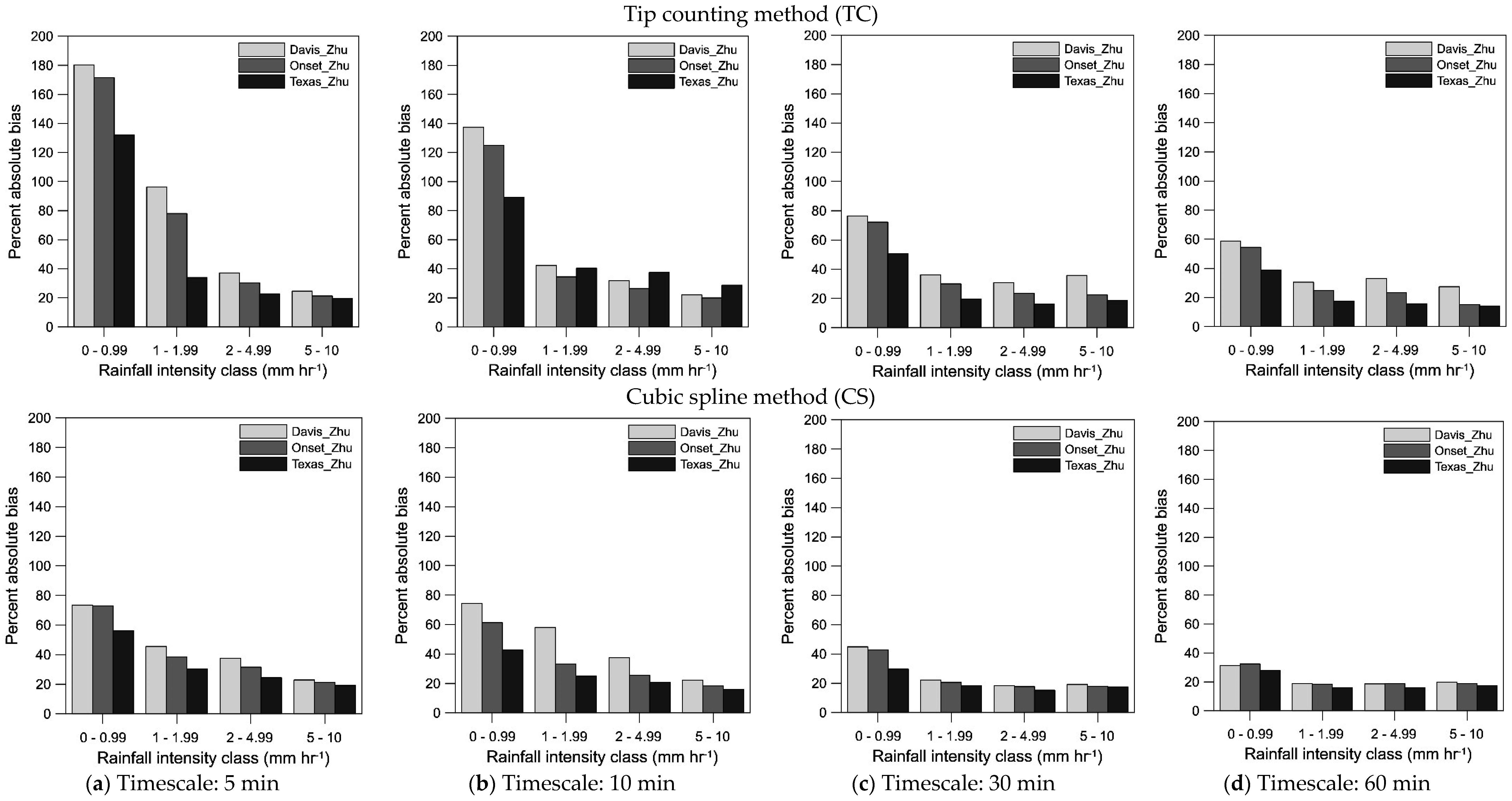
4.1. Effect of the Calculation Method for Rainfall Intensity, Rainfall Intensity Class, and Timescale on the Percent Absolute Bias

Figure 2 shows the value of the percent absolute bias of the DRTB gauges (Davis, Onset, and Texas) with respect to the LPM sensor in the Zhurucay observatory as a function of rainfall intensity, timescale, and rainfall intensity calculation method (TC or CS).
Results show that the error is inversely related to the timescale of data aggregation, with significant errors (up to 180%) for the timescales of 5 and 10 min. With respect to the magnitude of rainfall intensity, it was found that for the 5-min timescale, 95% of the rainfall intensities did not exceed 5 mm·h−1, 75% did not exceed 2 mm·h−1, and 50% did not exceed 1 mm·h−1. The error is highly dependent on the magnitude of the measured rainfall intensity, and on the method of calculation. Lower intensities (<2 mm·h−1) produced higher errors, which were significantly lower when the CS method was applied instead of the TC approach (maximum reduction of 100% and 50% for respectively the 0–1 and 1–2 mm·h−1 intensity classes).
The minimum Spearman correlation coefficients (ρ) between the calculated intensities and their references were respectively 0.85 and 0.87 for the TC and CS method. In fact, regardless of the method of calculation, the correlation is inversely related to the timescale of data, with higher correlations for the 30 and 60 min (up to 0.95) timescale. Hence, the error tends to increase when the timescale decreases. A reduction in error was observed when the timescale increases for both the TC and the CS methods, as shown in Figure 2. Furthermore, the data in this figure clearly illustrate that the percent absolute bias for the Davis_Zhu and Onset_Zhu rain gauges varies from 75% to 30% for rainfall intensities lower than 2 mm·h−1 and timescales of 5 and 10 min. For the Texas_Zhu rain gauge, percent absolute bias varies from 55% to 25%. Those results clearly show the difficulty in adequately measuring intensities with TB rain gauges in the páramo region, given the overall low rainfall intensities.

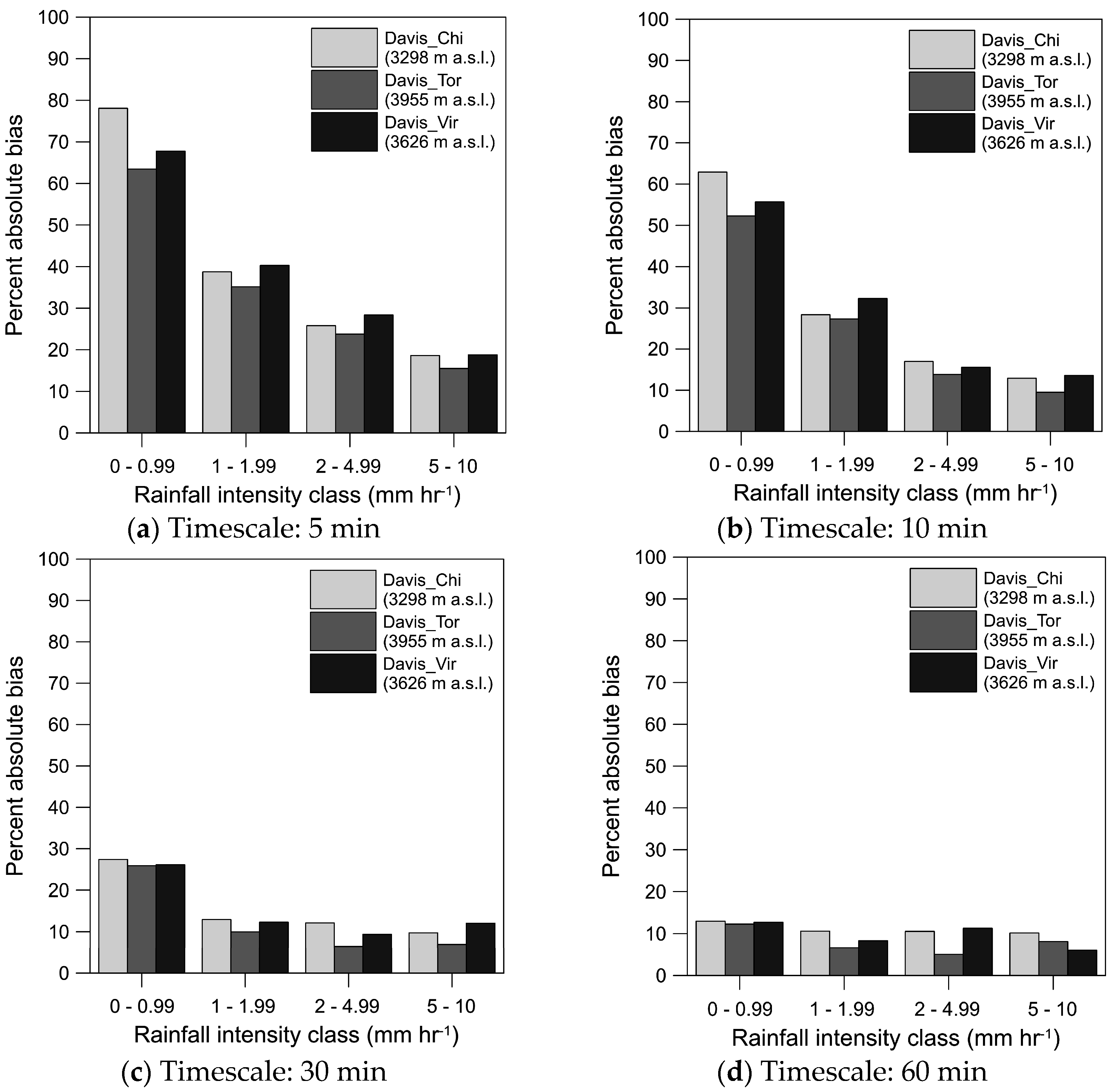
4.2. Effect of the Altitudinal Gradient

Figure 3 presents the notched box-whisker plot of daily rainfall (mm·day−1) constructed for 5-min rainfall measurements along an altitudinal gradient in the study area. The distribution of the daily rainfall in Toreadora (3955 m a.s.l.) corresponds very well with the distribution monitored in the Chirimachay site (3298 m a.s.l.) with 50% of daily rainfall less than or equal to 1.48 and 1.46 mm, 75% of the daily rainfall less than or equal to 4.55 and 4.99 mm, and 90% of the daily calculated rainfall depths less than or equal to 12 and 12.4 mm. The maximum recorded daily rainfall in both stations is respectively 27.76 and 26.92 mm. Daily rainfalls in the Virgen del Cajas site (3.626 m a.s.l.) are a bit lower with 50% of the events less than or equal to 1.05 mm, 75% of the daily rainfalls less than or equal to 3.76 mm·day−1, 90% less than or equal to 12.1 mm·day−1, and the maximum recorded daily rainfall depth was equal to 28.3 mm. The highest amount of rainfall that the lowest situated observation station (Chirimachay) received over the two-year study period was 2540 mm, which a bit higher than the total rainfall amount recorded in the highest situated station (Toreadora), 2407 mm. In the Virgen del Cajas station, situated at an elevation of 3620 m a.s.l. in between the two other stations, a total rainfall amount of 2140 mm was recorded. The total collected rainfall depth and distribution of daily rainfall depths in the three sites are not very different, supporting the hypothesis that there is no evidence of a significant difference in rainfall pattern along the altitudinal gradient.
Figure 4 shows the percent absolute bias of the Davis TB rain gauge with respect to the Texas TB rain gauge, used as reference along the altitudinal gradient. Analog to the findings in Zhurucay, significant errors were found at short timescales (5 and 10 min) and for low intensities (<2 mm·h−1). There is no relation between altitude, amount of precipitation, and error. In fact, comparing the three monitoring sites, results show that the range of errors for each timescale and intensity categories were lower than 20%. Moreover, similar error values (Davis compared to Texas rain gauges) were found when comparing the páramos of Zhurucay and Quinuas, indicating that there is not a clear influence of the altitudinal gradient on the magnitude of the error bias.
The average depth of rainfall events was 2 mm (63% of the events even less than 1 mm) and 1 mm, in the Zhurucay and Quinuas observatories. Furthermore, in Zhurucay, 80% of precipitation falls in the form of drizzle, whereas in Quinuas drizzle represents 95% of the precipitation. Notwithstanding, the overall low intensity of rainfall events in the study region, with storms of 1 mm or less, cannot be ignored in hydrological and meteorological models [35]. The study of [28] highlights that the use of TB rain gauges in the páramo region under-catches rainfall by not correctly intercepting drizzle rain. This issue also explains the high errors obtained when comparing intensities from TB rain gauges with the intensities from disdrometer data, regardless of the calculation method, and justifies for the study region the need for high-resolution precipitation monitoring sensors.
Ciach [20] found that the standard error for the TC method was three times the error for a linear interpolation method, considering a 10 mm·h−1 intensity and a 5-min timescale. Wang et al. [22] demonstrated that the CS algorithm is quantitatively better than the linear interpolation. It was found that in the páramo, the error for the TC method was 1.5 to 2 times the error for CS method, considering intensities lower than 10 mm·h−1 and a 5-min timescale. Consequently, the results of this study confirm that CS is a much more accurate method for calculating intensities.
Finally, contrary to the altitudinal distribution of the precipitation found by Rossenaar and Hofstede [16], the amount of precipitation did not equally decrease with increasing altitude. From this it might be concluded, as stated by Shi et al. [42], that in regions with large elevation variations, such as the Andes, high spatial variability of precipitation is likely dominated by local climate conditions (e.g., the orographic effect of the Andean Cordillera).

5. Conclusions

Analysis of the precipitation data, independent of the type of sensor, reveals the overall low intensity of precipitation events in the páramo ecosystem (50% of the rainfall intensities do not exceed 1 mm·h−1; 75% do not exceed 2 mm·h−1; and 95% of the intensities are less or equal to 5 mm·h−1). The error, measured by the percent absolute bias (without considering correction algorithms), is large for the TB rain gauges for rainfall intensities below 2 mm·h−1 and short timescales (5 to 10 min). The percent absolute bias of rainfall intensity for those intensities and timescales is considerably less when using the Cubic Spline (CS) method rather than the Tip Counting (TC) approach. The position of the rain gauge along an altitudinal gradient has no significant effect on the calculated error; in fact, there is no relation between altitude, cumulative rainfall depth, and error value.
Monitoring with TB rain gauges with a resolution of 0.1 mm or less results in a significant reduction of the uncertainty. Our findings support the suggestion that accurate monitoring of rainfall in the Andean region requires the use of high-resolution rainfall equipment. Implementation involves a step-wise replacement of the existing infrastructure of tipping-bucket rain gauges by high resolution laser precipitation sensors. A more accurate measurement of precipitation, a crucial input in most hydrological models, might lead to a better understanding of the complex hydrology of the páramo ecoregion. Nevertheless, despite a reduction of errors, uncertainty remains to be considered in decision-making of water management resources problems.

Acknowledgments

The research was funded by the Research Office of the University of Cuenca (DIUC) and the Empresa Pública Municipal de Telecomunicaciones, Agua potable, Alcantarillado y Saneamiento de Cuenca (ETAPA EP) via the project “Identification of hydro-meteorological processes that trigger extreme floods in the city of Cuenca using precipitation radar”. We would like to especially acknowledge the valuable support of Ryan Padrón regarding the correct use of the laser disdrometer and in providing constructive ideas. Thanks are due to DIUC for covering the costs associated with the dissemination of the results. The authors are grateful to the three anonymous reviewers whose detailed comments contributed greatly to the improvement of this paper.

Author Contributions

Paul Muñoz analyzed the data and wrote the manuscript. Jan Feyen contributed to the data analyses and provided a critical revision of the manuscript. Rolando Célleri designed and supervised the study, and provided a critical revision of the manuscript.

Conflicts of Interest

The authors declare no conflict of interest. The founding sponsors had no role in the design of the study; in the collection, analyses, or interpretation of data; in the writing of the manuscript, and in the decision to publish the results.

Abbreviations

The following abbreviations are used in this manuscript:
TBTipping Bucket
DRTBDifferent Resolution Tipping Buckets
TCTip Counting
CSCubic Spline.

References

  1. González, J.; Lajara, J.; Díaz, S. Errors Analysis in extreme rainfall recording due to tipping bucket rain gauge performance. In Proceedings of the 36th IAHR World Congress, The Hague, The Netherlands, 28 June–3 July 2015.
  2. Buytaert, W.; Célleri, R.; De Bièvre, B.; Cisneros, F.; Wyseure, G.; Deckers, J.; Hofstede, R. Human impact on the hydrology of the Andean páramos. Earth-Sci. Rev. 2006, 79, 53–72. [Google Scholar] [CrossRef] [Green Version]
  3. Dinerstein, E.; Graham, D.J.; Olsen, D.M.; Webster, A.; Primm, S.; Bookbinder, M.; Ledec, G. Una Evaluación del Estado de Conservación de las Eco-Regiones Terrestres de América Latina y el Caribe; Banco Internacional de Reconstrucción y Fomento/Banco Mundial: Washington, DC, USA; World Wildlife Fund: Washington, DC, USA, 1995. [Google Scholar]
  4. Sarmiento, L.; Lambí, L.D.; Escalona, A.; Márquez, N. Vegetation patterns, regeneration rates and divergence in an old field-succession of the high tropical Andes. Plant Ecol. 2003, 166, 63–74. [Google Scholar] [CrossRef]
  5. Célleri, R.; Feyen, J. The Hydrology of Tropical Andean Ecosystems: Importance, Knowledge Status, and Perspectives. Mt. Res. Dev. 2009, 29, 350–355. [Google Scholar] [CrossRef] [Green Version]
  6. Buytaert, W.; Cuesta-Camacho, F.; Tobón, C. Potential impacts of climate change on the environmental services of humid tropical alpine regions. Glob. Ecol. Biogeogr. 2011, 20, 19–33. [Google Scholar] [CrossRef]
  7. Messerli, B.; Viviroli, D.; Weingartner, R. Mountains of the world: Vulnerable water towers for the 21st century. Ambio 2004, 13, 29–34. [Google Scholar]
  8. Kumar, S.; Gill, G.S.; Santosh, S. Spatial Distribution of Rainfall with Elevation in Satluj River Basin: 1986–2010, Himachal Pradesh, India. Int. Lett. Chem. Phys. Astron. 2015, 57, 163. [Google Scholar] [CrossRef]
  9. Alijani, B. Effect of the Zagros Mountains on the spatial distribution of precipitation. J. Mt. Sci. 2008, 5, 218–231. [Google Scholar] [CrossRef]
  10. Buytaert, W.; Celleri, R.; Willems, P.; De Bièvre, B.; Wyseure, G. Spatial and temporal rainfall variability in mountainous areas: A case study from the south Ecuadorian Andes. J. Hydrol. 2006, 329, 413–421. [Google Scholar] [CrossRef] [Green Version]
  11. Celleri, R.; Willems, P.; Buytaert, W.; Feyen, J. Space-time rainfall variability in the Paute Basin, Ecuadorian Andes. Hydrol. Process. 2007, 21, 3316–3327. [Google Scholar] [CrossRef]
  12. Espinoza Villar, J.C.; Ronchail, J.; Guyot, J.L.; Cochonneau, G.; Naziano, F.; Lavado, W.; De Oliveira, E.; Pombosa, R.; Vauchel, P. Spatio-temporal rainfall variability in the Amazon basin countries (Brazil, Peru, Bolivia, Colombia, and Ecuador). Int. J. Climatol. 2009, 29, 1574–1594. [Google Scholar] [CrossRef]
  13. De Biévre, B.; Iñiguez, V.; Buytaert, W. Hidrología del Páramo. Importancia, propiedades y vulnerabilidad. In Investigaciones Biofísicas en el Páramo, No. 21; GTP/Abya Yala: Quito, Ecuador, 2006. [Google Scholar]
  14. Rollenbeck, R.; Bendix, J. Rainfall distribution in the Andes of southern Ecuador derived from blending weather radar data and meteorological field observations. Atmos. Res. 2011, 99, 277–289. [Google Scholar] [CrossRef]
  15. Ochoa-Tocachi, B.F.; Buytaert, W.; De Bièvre, B.; Célleri, R.; Crespo, P.; Villacís, M.; Llerena, C.A.; Acosta, L.; Villazón, M.; Guallpa, M.; et al. Impacts of land use on the hydrological response of tropical Andean catchments. Hydrol. Process. 2016, 30, 4074–4089. [Google Scholar] [CrossRef]
  16. Rossenaar, A.J.G.A.; Hofstede, R.G.M. Effects of burning and grazing on root biomass in the páramo ecosystem. In Páramo: An Andean Ecosystem Under Human Influence; Balslev, H., Luteyn, J.L., Eds.; Academic Press: London, UK, 1992; pp. 211–213. [Google Scholar]
  17. World Meteorological Organisation. World Hydrological Cycle Observing System Guidelines; World Meteorological Organisation: Geneva, Switzerland, 2015; p. 87. [Google Scholar]
  18. Lanza, L.G.; Vuerich, E. The WMO field intercomparison of rain intensity gauges. Atmos. Res. 2009, 94, 534–543. [Google Scholar] [CrossRef]
  19. Organización Meteorológica Mundial. Guía de Prácticas Hidrológicas; Organización Meteorológica Mundial: Geneva, Switzerland, 2008; OMM-NO. 168; p. 324. [Google Scholar]
  20. Ciach, G.J. Local random errors in tipping-bucket rain gauge measurements. J. Atmos. Ocean. Technol. 2003, 20, 752–759. [Google Scholar] [CrossRef]
  21. Habib, E.; Krajewski, W.F.; Kruger, A. Sampling Errors of Tipping-Bucket Rain Gauge Measurements. J. Hydrol. Eng. 2001, 6, 159–166. [Google Scholar] [CrossRef]
  22. Wang, J.; Fisher, B.L.; Wolff, D.B. Estimating rain rates from tipping-bucket rain gauge measurements. J. Atmos. Ocean. Technol. 2008, 25, 43–56. [Google Scholar] [CrossRef]
  23. Michaelides, S.C. Precipitation: Advances in Measurement, Estimation and Prediction; Springer Science & Business Media: Berlin, Germany, 2008. [Google Scholar]
  24. Nystuen, J.A.; Proni, J.R.; Black, P.G.; Wilkerson, J.C. A comparison of automatic rain gauges. J. Atmos. Ocean. Technol. 1996, 13, 62–73. [Google Scholar] [CrossRef]
  25. Padrón, R.S.; Wilcox, B.P.; Crespo, P.; Célleri, R. Rainfall in the Andean Páramo: New Insights from High-Resolution Monitoring in Southern Ecuador. J. Hydrometeorol. 2015, 16, 985–996. [Google Scholar] [CrossRef]
  26. Liu, X.C.; Gao, T.C.; Liu, L. A comparison of rainfall measurements from multiple instruments. Atmos. Meas. Tech. 2013, 6, 1585–1595. [Google Scholar] [CrossRef]
  27. Upton, G.; Brawn, D. An investigation of factors affecting the accuracy of Thies disdrometers. In Proceedings of WMO Technical Conference on Instruments and Methods of Observation (TECO-2008), St. Petersburg, Russia, 27–29 November 2008; pp. 1–9.
  28. Nešpor, V.; Sevruk, B. Estimation of wind-induced error of rainfall gauge measurements using a numerical simulation. J. Atmos. Ocean. Technol. 1999, 16, 450–464. [Google Scholar] [CrossRef]
  29. Lanzinger, E. Rainfall amount and intensity measured by the Thies laser precipitation monitor. In Proceedings of the WMO Technical Conference on Instruments and Methods of Observation (TECO-2006), Geneva, Switzerland, 7–14 December 2006; pp. 1–9.
  30. Williams, R.G.; Erdman, M.D. Low-cost computer interfaced rain gauge. Comput. Electron. Agric. 1987, 2, 67–73. [Google Scholar] [CrossRef]
  31. Sadler, E.J.; Busscher, W.J. High-intensity rainfall rate determination from tipping-bucket rain gauge data. Agron. J. 1989, 81, 930–934. [Google Scholar] [CrossRef]
  32. Peleg, N.; Ben-Asher, M.; Morin, E. Radar subpixel-scale rainfall variability and uncertainty: Lessons learned from observations of a dense rain-gauge network. Hydrol. Earth Syst. Sci. 2013, 17, 2195–2208. [Google Scholar] [CrossRef]
  33. Colli, M.; Lanza, L.G.; Chan, P.W. Co-located tipping-bucket and optical drop counter RI measurements and a simulated correction algorithm. Atmos. Res. 2013, 119, 3–12. [Google Scholar] [CrossRef]
  34. Costello, T.A.; Williams, H.J. Short duration rainfall intensity measured using calibrated time-of-tip data from a tipping bucket raingage. Agric. For. Meteorol. 1991, 57, 147–155. [Google Scholar] [CrossRef]
  35. Al-Wagdany, A.S. Evaluation of Dual Tipping-Bucket Rain Gauges Measurement in Arid Region Western Saudi Arabia. Arab. J. Sci. Eng. 2014, 40, 171–179. [Google Scholar] [CrossRef]
  36. World Meteorological Organisation. Guide to Meteorological Instruments and Methods of Observation; World Meteorological Organisation: Geneva, Switzerland, 2010. [Google Scholar]
  37. Tokay, A.; Wolff, D.B.; Wolff, K.R.; Bashor, P. Rain gauge and disdrometer measurements during the Keys Area Microphysics Project (KAMP). J. Atmos. Ocean. Technol. 2003, 20, 1460–1477. [Google Scholar] [CrossRef]
  38. Mosquera, G.M.; Lazo, P.X.; Célleri, R.; Wilcox, B.P.; Crespo, P. Runoff from tropical alpine grasslands increases with areal extent of wetlands. Catena 2015, 125, 120–128. [Google Scholar] [CrossRef]
  39. Shedekar, V.S.; King, K.W.; Fausey, N.R.; Soboyejo, A.B.O.; Harmel, R.D.; Brown, L.C. Assessment of measurement errors and dynamic calibration methods for three different tipping bucket rain gauges. Atmos. Res. 2016, 178–179, 445–458. [Google Scholar] [CrossRef]
  40. Vasvári, V. Calibration of tipping bucket rain gauges in the Graz urban research area. Atmos. Res. 2005, 77, 18–28. [Google Scholar] [CrossRef]
  41. Nystuen, J.A. Relative performance of automatic rain gauges under different rainfall conditions. J. Atmos. Ocean. Technol. 1999, 16, 1025–1043. [Google Scholar] [CrossRef]
  42. Shi, H.; Li, T.; Wei, J.; Fu, W.; Wang, G. Spatial and temporal characteristics of precipitation over the Three-River Headwaters region during 1961–2014. J. Hydrol. Reg. Stud. 2016, 6, 52–65. [Google Scholar] [CrossRef]
Figure 1. Rainfall intensity distribution in the páramos of Zhurucay and Quinuas.
Water 08 00534 g001
Figure 2. Percent absolute bias of the collocated tipping-bucket (TB) rain gauges Davis, Onset, and Texas with respect to the LPM sensor as a function of rainfall intensity class and timescale, respectively calculated with the tip counting (TC) (top) and the cubic spline (CS) method (bottom).
Water 08 00534 g002
Figure 3. Notched Box-Whisker plot (which displays the population range of the daily rainfall depths, showing respectively the minimum, maximum, median, lower quartile, and upper quartile, and the outliers (black dots).) of the daily rainfall distribution (mm·day−1) in three stations along an altitudinal gradient, for the experimental period of January 2014 to February 2016.
Water 08 00534 g003
Figure 4. Percent absolute bias calculated with the CS method of the Davis with respect to the Texas TB rain gauge for different rainfall intensity classes and timescales, along an altitudinal gradient.
Water 08 00534 g004
Table 1. Sensors, available data intervals, and data gap percentage of the sensors used in each study area.
Study AreaSensorAvailable DataNumber of Events% Missing Data
SinceTo
Zhurucay observatoryDavis_Zhu21/02/201114/02/20149534
Onset_Zhu21/02/201104/01/201411337
Texas_Zhu21/02/201119/03/201416584
LPM21/02/201101/10/2012 4
09/11/201219/03/2014
Quinuas observatoryDavis_Chi22/01/201405/02/20166815
Texas_Chi22/01/201405/02/201611150
Davis_Tor16/01/201406/04/201557311
09/05/201529/06/2015
29/07/201505/02/2016
Texas_Tor16/01/201405/02/201612050
Davis_Vir20/01/201419/08/20155035
Texas_Vir20/01/201405/02/201610440

