Article

Spatio-Temporal Analysis of Water Quality Parameters in Machángara River with Nonuniform Interpolation Methods

by
Iván P. Vizcaíno
1,*,
Enrique V. Carrera
1,
Margarita Sanromán-Junquera
2,
Sergio Muñoz-Romero
2,
José Luis Rojo-Álvarez
2 and
Luis H. Cumbal
3
1
Departamento de Eléctrica y Electrónica, Universidad de las Fuerzas Armadas ESPE, Av. General Rumiñahui s/n, P.O. Box 171-5-231B, Sangolquí, Ecuador
2
Department of Signal Theory and Communications and Telematic Systems and Computation, Universidad Rey Juan Carlos, Camino del Molino S/N, 28942 Fuenlabrada, Madrid, Spain
3
Centro de Nanociencia y Nanotecnología, Universidad de las Fuerzas Armadas ESPE, Av. General Rumiñahui s/n, P.O. Box 171-5-231B, Sangolquí, Ecuador
*
Author to whom correspondence should be addressed.
Water 2016, 8(11), 507; https://doi.org/10.3390/w8110507
Submission received: 25 July 2016 / Revised: 24 October 2016 / Accepted: 28 October 2016 / Published: 4 November 2016

Abstract

:
Water quality measurements in rivers are usually performed at intervals of days or months in monitoring campaigns, but little attention has been paid to the spatial and temporal dynamics of those measurements. In this work, we propose scrutinizing the scope and limitations of state-of-the-art interpolation methods aiming to estimate the spatio-temporal dynamics (in terms of trends and structures) of relevant variables for water quality analysis usually taken in rivers. We used a database with several water quality measurements from the Machángara River between 2002 and 2007 provided by the Metropolitan Water Company of Quito, Ecuador. This database included flow rate, temperature, dissolved oxygen, and chemical oxygen demand, among other variables. For visualization purposes, the absence of measurements at intermediate points in an irregular spatio-temporal sampling grid was fixed by using deterministic and stochastic interpolation methods, namely, Delaunay and k-Nearest Neighbors (kNN). For data-driven model diagnosis, a study on model residuals was performed comparing the quality of both kinds of approaches. For most variables, a value of k = 15 yielded a reasonable fitting when Mahalanobis distance was used, and water quality variables were better estimated when using the kNN method. The use of kNN provided the best estimation capabilities in the presence of atypical samples in the spatio-temporal dynamics in terms of leave-one-out absolute error, and it was better for variables with slow-changing dynamics, though its performance degraded for variables with fast-changing dynamics. The proposed spatio-temporal analysis of water quality measurements provides relevant and useful information, hence complementing and extending the classical statistical analysis in this field, and our results encourage the search for new methods overcoming the limitations of the analyzed traditional interpolators.

1. Introduction

Pollution is related to the introduction into the environment of substances, from anthropogenic or natural origin, which are harmful or toxic to humans and ecosystems. Pollution usually alters the chemical, physical, biological, or radiological integrity of soil, water, and living species, resulting in alterations of the food chain, with effects on human health [1,2]. In particular, water pollution is mainly due to the increment in urban and industrial density. Growing population waste poses a threat to public health and jeopardizes the continuous use of water reserves [3]. For example, contamination of watercourses is a consequence of wastewater discharge, from municipal, industrial, or farming runoffs [4]. Typically, urban wastewater is a complex mixture containing water (usually over 99%) mixed with organic and inorganic compounds, both in suspension and dissolved with very small concentrations (mg/L) [5]. Globally, two million tons of wastewater are discharged into the world waterways [6]. Wastewater Treatment Plants (WWTPs) are used to combat water pollution of rivers in communities (municipalities) reducing suspended solids and the organic load to accelerate the natural process of water purification [3,7].
On the other hand, several properties and factors are usually considered in the water quality analysis and in the monitoring of pollution water sources in order to assess the impact of water pollution on flora, fauna, and humans. Water appearance, color or turbidity, temperature, taste, and smell often describe the physical properties of drinking water, whereas the water chemical characterization includes the analysis of organic and inorganic substance concentrations. Microbiological features are related to pathogenic agents (bacteria, viruses, and protozoa), which are relevant to public health and usually modify the water chemistry. In addition, radiological factors could be also considered in areas where water comes into contact with radioactive substances [8]. Other specifications such as water hardness, pH, acidity, oils, and fats can also be taken into account in the water quality analysis.
Water quality monitoring focuses on programmed sampling, measurement, and recording of regulated water quality parameters. The water quality management in rivers can be more efficient when: (1) monitoring of rivers is continuous, hence its seasonal behavior can be characterized; (2) the sampling period is based on the spatio-temporal dynamics (trends or patterns) of the measured variables; (3) the choice of the sampling sites takes into account the basin irregularities; and (4) other factors at the study area are taken into consideration, such as population and industrial growth. Measurements are not usually taken uniformly at determined locations and times during the monitoring campaigns, and the pollutant concentrations in river waters do not follow linear variations. Therefore, the use of mathematical models with basic physics (that govern the transport process of pollution) and linear models can be complemented with data-driven models for modeling the river contaminants dynamics, in the sense of trends and spatio-temporal structures [9].
For these reasons, several scientific works have scrutinized different spatio-temporal analysis of water quality from a statistical point of view, in order to understand their behavior and help to generate water decontamination designs in a more efficient way. Siyue et al. analyzed up to 41 sites at the Han River (China) during 2005 and 2006 in order to explore the spatio-temporal variations in the basin [10]. Cluster methods and analysis of variance (ANOVA) grouped the 41 sampling sites into five statistically significant clusters. Results showed that dissolved inorganic nitrogen and nitrates had large spatial variability, while nitrogen had a relatively higher concentration in wet seasons compared with dry seasons, and phosphorous had the opposite trend. On the other hand, Serre et al. used the Bayesian maximum entropy to analyze spatio-temporal variability of water quality parameters in the case of phosphate estimation along the Raritan River basin (New Jersey, USA) between 1990 and 2002 [11]. The database consisted of 1305 phosphate measurements at 55 monitoring stations. Their results showed that the spatio-temporal analysis improves the purely spatial analysis when the water samples are noisy and scarce. In addition, Duan et al. proposed a statistical multivariate analysis including cluster analysis, discriminant analysis and principal component analysis/factor analysis to distinguish spatio-temporal variation of water quality and contaminants [12]. Fourteen parameters were studied in 28 sites of Eastern Poyang Lake Basin, Jiangxi Province of China from January 2012 to April 2015. This work also pointed out the spatio-temporal analysis as a tool to help in the optimization of the water quality monitoring programs. The impact of wastewater was also scrutinized in a detailed anthropogenic study of the Henares River (Spain) [13]. The Henares River runs through residential, industrial, and farming areas. Thus, strategic points were chosen along the river, with five stations upstream of a WWTP, and five stations downstream. Six monitoring campaigns were carried out between April and June 2010, assembling 36 water samples altogether. Descriptive statistics, such as frequency or mean of pollutant concentration and uni-dimensional graphical representations were used to analyze their spatial and temporal evolution, showing the influence of the wastewater discharge and of the farm areas’ proximity. For example, high concentrations of polycyclic aromatic hydrocarbons, which are usually adsorbed on the river sediments, still continued along the Henares River regardless of season. Note that all these results point out the relevance of the observable dynamics of these pollutants with respect to time and space. This work pointed out the importance of the spatio-temporal analysis in order to visualize the trends of some compounds in the rivers, which could determine a possible relationship between river water contamination and wastewater effluent discharges.
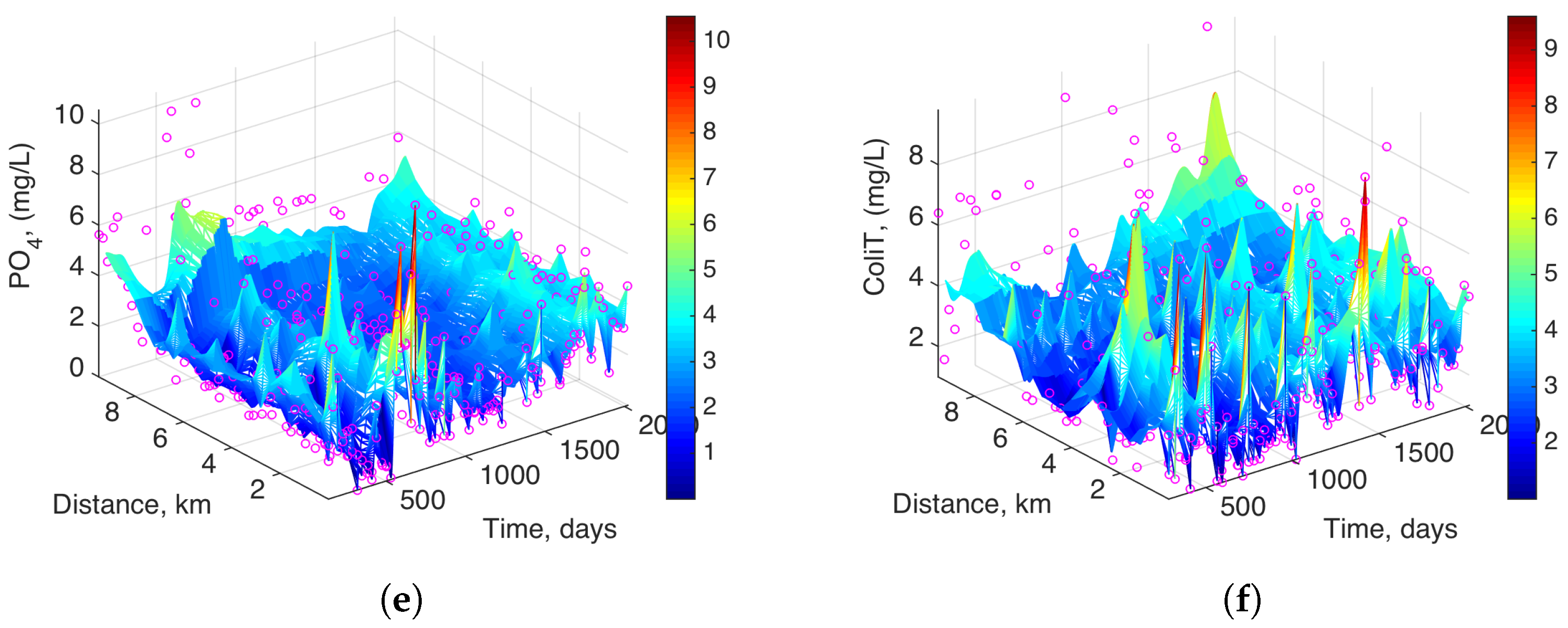
However, and to the best of our knowledge, the variability of measurements jointly expressed in space and time has not been explored for analyzing the spatio-temporal distributions of water quality variables. In the present work, we propose scrutinizing the scope and limitations of state-of-the-art interpolation methods aiming to estimate the spatio-temporal dynamics (in terms of trends and structures) of relevant variables for water quality analysis usually taken in rivers. For visualization purposes, the absence of measurements at intermediate points in an irregular spatio-temporal sampling grid is fixed by using deterministic and stochastic interpolation methods, namely, Delaunay and k-Nearest Neighbors (kNN). For data-driven model diagnosis, a study on model residuals is performed, allowing for comparison of the model quality for both kinds of approaches.
These methods are here applied to pollution measurements at the Machángara River and its tributaries in Quito, Ecuador. Whereas several previous studies of Machángara River pollution have been made since 1977 [14], they have conducted statistical analysis on specific variables such as phosphates, pesticides, nitrates, and hydrocarbons, but a more detailed and complete view of the wastewater dynamics can still be addressed.
The rest of this paper is as follows. In Section 2, the materials and methods are explained, including the mathematical description of the interpolation algorithms and details of the database used for this analysis. In Section 3, results are presented for a number of measured variables, the algorithmic performance is benchmarked, a comparative analysis is made on the data-driven residuals of the models with both methods, and the analysis on several environmental variables and their spatio-temporal dynamics is described. In Section 4, the results are discussed, and in Section 5, the main conclusions are presented.

2. Materials and Methods

2.1. Study Area

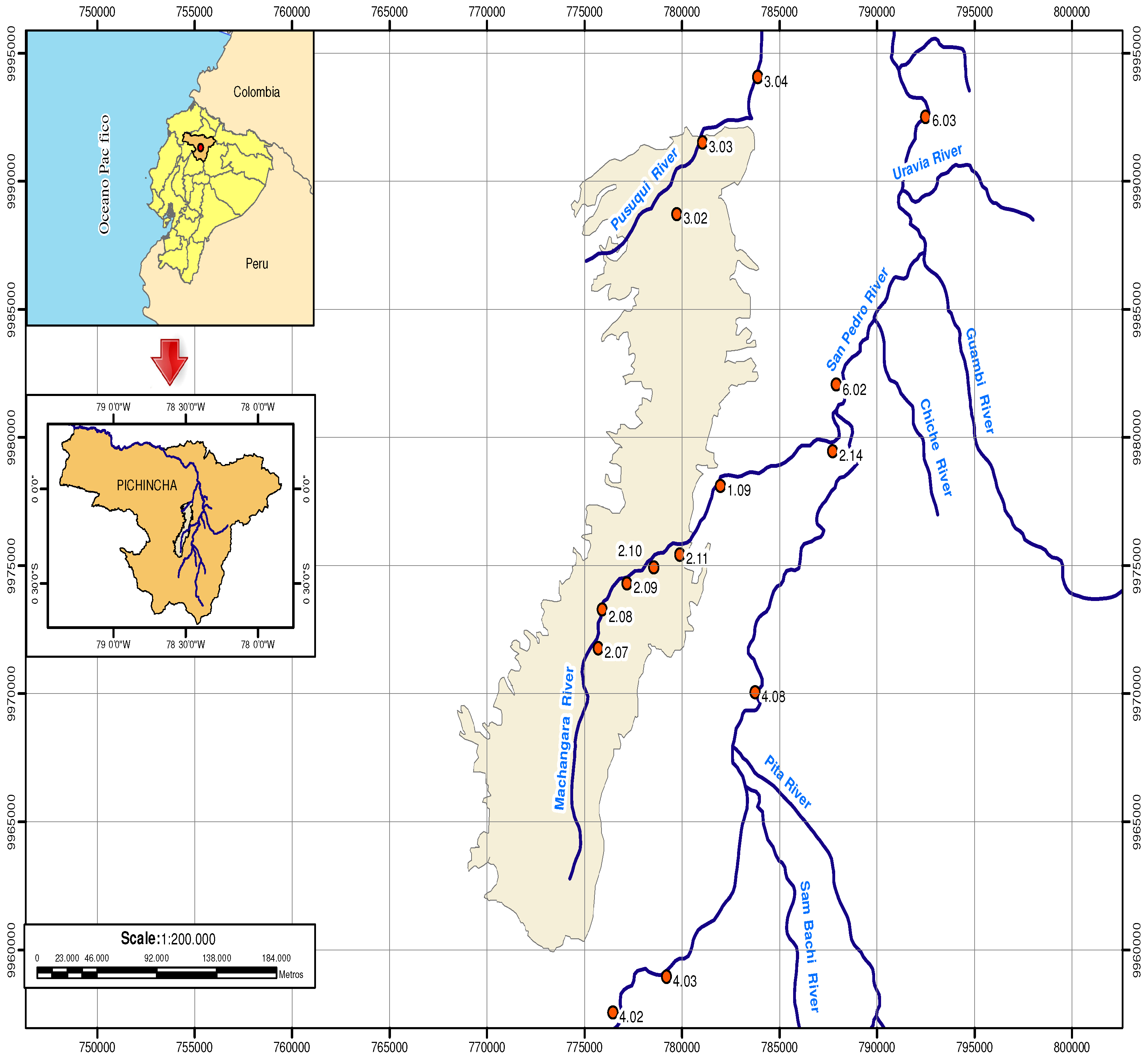
Quito, the capital of Ecuador, is located at approximately 2815 m above sea level, at UTMWGS84 coordinates with latitude 9973588.50 [00°13 47 S] and longitude 776529.41 [78°31 30 W], as depicted in Figure 1, and it had an average temperature of 14 °C between 2002 and 2007. The Machángara River was chosen for this study because it is the main wastewater collector of Quito. This river runs through the city from south to north, collecting wastewater at a distance of approximately 22 km, and it receives about 75% of the city waste. Along the river pathway, 25 water quality monitoring stations are installed [14,15]. For our work, six stations were chosen in the upstream section of the River, within a reach of about 10 km, in order to monitor large amounts of wastewater. The identification of the monitoring stations is shown in Table 1, and the water quality parameters to be analyzed are described in Table 2.
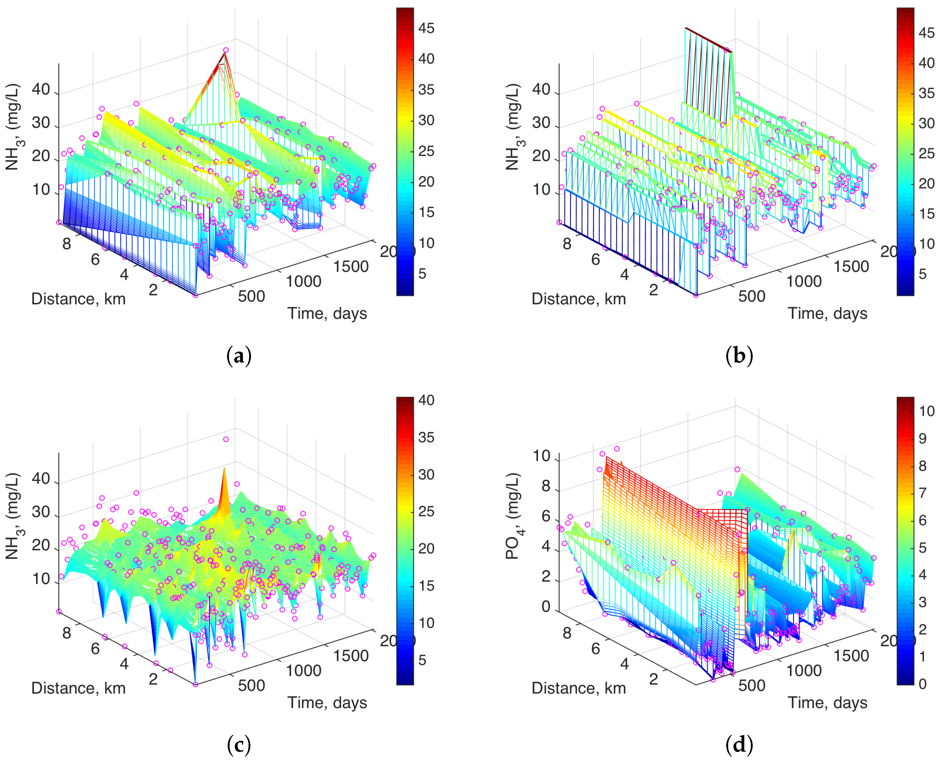
Sixty-four monitoring campaigns were carried out to measure 15 water quality parameters between 2002 and 2007. Note that a value of each parameter is usually collected in each campaign. However, some water quality parameters are sometimes not collected, and also more than one value can be registered in several campaigns. The number of water quality measurements available for each variable is shown in Table 3. In the same time period, rainfall measurements were conducted at one weather station near the study area, and these measurements were assembled to compare rainfall with water quality variables at the Machángara River.
The preprocessing of the water quality database required the design of the following modules in Matlab™ (R2014b, TheMathWorks Inc., Natick, MA, USA): (1) station selection, which allowed the graphical selection of water quality monitoring stations from a map of Quito and those measurements; and (2) model estimation with smoothing interpolation methods and its representations, which allows us to work with the database of the selected monitoring stations in specific sections along the Machángara River. The latter module also helped to calculate the Mean Absolute Error (MAE) for the two studied interpolation algorithms, namely, Delaunay and kNN algorithms.

2.2. Interpolation Algorithms

Our aim in the present work is to show that statistical interpolation can yield relevant information on the underlying dynamics of the analyzed variables, which can complement the current knowledge and analysis of measurements themselves. The proposed interpolation techniques not only improve data visualization, but they also allow the identification of trends and structures that are consistently supported by measurements being close in time or space. The result of such an interpolation process can provide an enhanced information view for assisting water analysts. Note that we are actually working here with two conventional and well-known approaches, namely, deterministic interpolation (given by Delaunay) and statistical interpolation (given by kNN). The first one does not provide more than just a grid visualization of time-spatial data, and the second one is well known in the machine learning literature for being able to provide us with the dynamics or trends in the underlying evolution of the measured variables. As a result, these trends are more easily and consistently observed in statistical interpolation approaches, especially when noise and perturbations are clearly present in the measurements. Note that, in this case, the interpolation process can be seen as a smoothing estimation process, which identifies the consistent trends and separates them from the system perturbations, as estimated by the model residuals.
In studies about multi-dimensional variables, it can be useful to search for dependencies among them; therefore, the construction of mathematical models should be able to describe those existing relationships. Regression models can explain the dependency relationship between a response variable and one or more independent or explanatory variables in such a way that these models can estimate new values from a new unobserved set of measurements from the explanatory variables.
The use of nonparametric regression is sometimes suitable when a response is difficult to obtain in terms of physical models or when the measuring methods are expensive. The main objective of the interpolation is to estimate one or more unknown independent variables from a given set of simultaneously measured samples from the independent variables and the response variable.
An intermediate goal in this work is to fill up the regular grid in the quantitative representation of water quality measurements at those times when no monitoring campaigns were conducted, and in those spaces of rivers where there are no monitoring stations. The interpolation methods used in this work were Delaunay Triangulation and kNN.

2.2.1. Interpolation with Delaunay Triangulation

The interpolation with Delaunay triangulation has been used in digital cartography for the generation of digital terrain models [16]. The starting point of this method is a cloud of three-dimensional (3D) points, usually irregularly spatial distributed, which allows us to represent surfaces digitally. This triangulation approximates surfaces by irregular and planar triangles that connect the 3D points. In this work, we do not use the 3D spatial coordinates of the points as input space, but instead we pursue a representation for two-dimensional input spaces given by the time and location (in terms of the distance along the river path), where a measurement was taken.
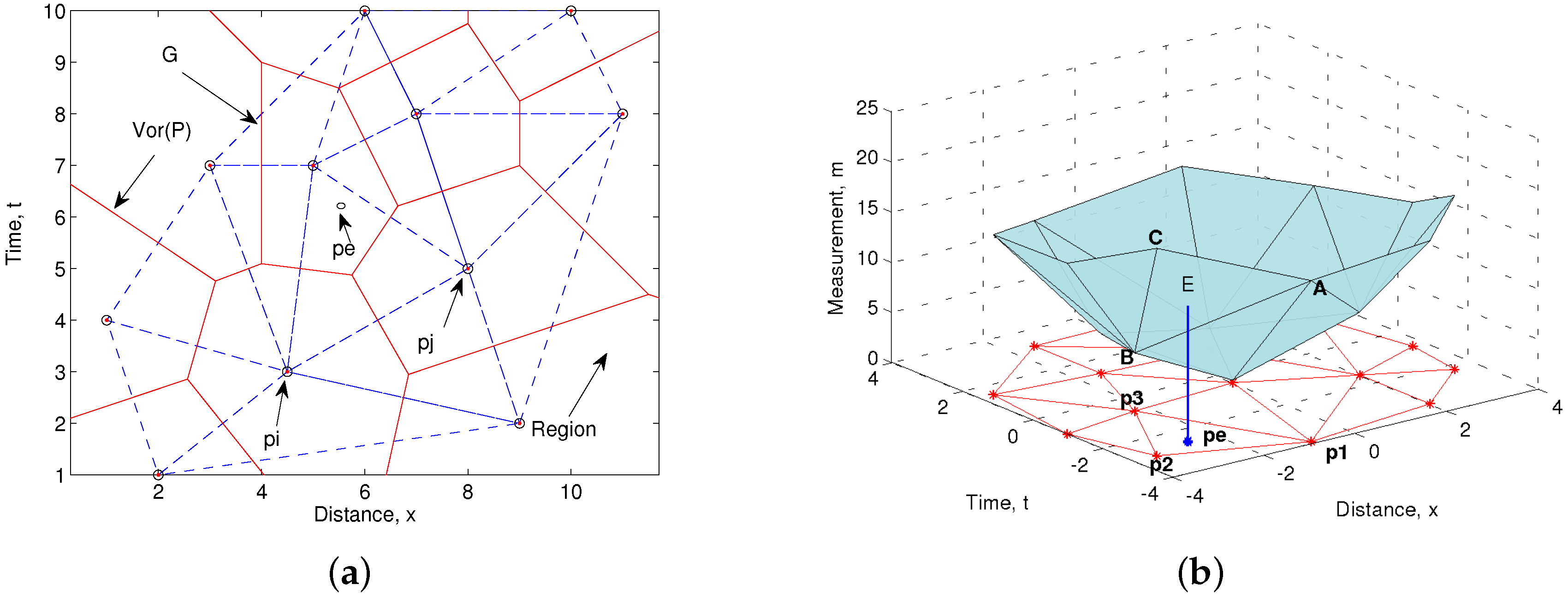
The Delaunay interpolation method is based on Voronoi diagrams and Delaunay triangulation, which uses the Euclidean distance as interpolation criterion [17]. Given two points in the spatio-temporal plane ( x , t ) , denoted as p 1 = ( x 1 , t 1 ) and p 2 = ( x 2 , t 2 ) , the Euclidean distance among them is
d i s t ( p 1 , p 2 ) : = ( x 1 x 2 ) 2 + ( t 1 t 2 ) 2 .
Let P = { p 1 , p 2 , . . . , p n } be a set of n distinct points (or sites) in the spatio-temporal plane. The Voronoi diagram of P is the subdivision of the plane in n cells (Figure 2a), one for each site in P. The condition is that a point p e lies in the cell corresponding to a site p i if and only if d i s t ( p e , p i ) < d i s t ( p e , p j ) for each p j P with j i . The Voronoi diagram of P is denoted by V o r ( P ) , and it indicates only the edges and vertices of the subdivision p i [17]. Graph G has a node for every Voronoi cell equivalent for every site, and the union of external edges for each G conforms a polygon Pol.
Figure 2b shows the measurements (m axe) of a variable which forms a polyhedron of irregular triangles where the measurements are the vertices. Note that bold uppercases are used to represent points (vertices of irregular triangles which form a polyhedron) defined in the coordinates ( x , t , m ) , while the projections of these vertices in the plane ( x , t ) are represented by bold lowercases. For example, samples represented by points A , B , and C form a triangle polyhedron, and when it is projected in the plane ( x , t ) , a new triangle with p 1 , p 2 , and p 3 vertices is formed. The estimated value, m E ^ , at a new point E = ( x E , t E ) , is obtained two-fold: (1) a Delaunay triangle, which encloses the point E , is found; and (2) m E ^ is computed as the results of applying the values x E and t E in the plane equation defined by the points A , B and C in the linear interpolation, and as the m E value of the nearest neighbor vertex in the nearest interpolation.

2.2.2. kNN Interpolation

The kNN rule is among the simplest statistical learning tools in density estimation, classification, and regression. Trivial to train and easy to code, the nonparametric algorithm is surprisingly competitive and fairly robust to errors when using cross-validation procedures [18]. The fitting is made by using only those measurements close to the target point p e . A function of weights assigned to each p i is based on the distance from p e .
The usual calculation methods of known distances are Euclidean, Manhattan, Minkowski, weighted Euclidean, Mahalanobis, and Cosine, among others. The Mahalanobis distance between two points p 1 and p 2 is defined as
d i s t M ( p 1 , p 2 ) = ( p 1 p 2 ) 1 ( p 1 p 2 ) ,
where ∑ is the covariance matrix. Mahalanobis distance has advantageous properties compared to the use of Euclidean distance, namely, it is invariant to changes in scale, and it does not depend on measurements units. By using matrix 1 , we consider correlations between variables and redundancy effect. The estimation function of p e is represented by f ^ ( p e ) , and it is estimated according to Distance Weighted Nearest Neighbor algorithm as
f ^ ( p e ) = i = 1 k w i f ( p i ) i = 1 k w i ,
where f ( p i ) represents the samples near p e , and w i is the weights function that is defined in terms of Mahalanobis distance as
w i = 1 d i s t M ( p e , p i ) 2 .

2.3. Performance Measures

The goal of any data-driven methodology is to estimate (learn) a useful model of the unknown system from available data. A criteria related to usefulness is the prediction accuracy (generalization), related to the capability of the model to provide accurate estimates for future data. In the learning problem, the goal is to estimate a function by using a finite number of training samples. The availability of a finite number of training samples implies that any estimate of an unknown function is often inaccurate. In regression learning problems, we can obtain a measurement of the performance in terms of the generalization capabilities of the model, with the goal of minimizing the empirical risk as described below [19].
Given D = ( x i , t i , m i ) i = 1 n as the training set, the pairs ( x i , t i ) are identified as inputs and ( m i ) as outputs, where x represents the distance, t is time, and m is any water quality measurement. The basic goal of supervised learning is to use the training set D to learn a function f ^ (in the hypothesis space H) that evaluates at a new pair ( x , t ) and estimates its associated value ( m ) .
In order to measure the quality of f ^ function, we use a loss function denoted by l ( f ^ , D ) . The estimation for a given ( x , t ) is f ^ ( x , t ) , and the true value is ( m ) . One of the loss functions used in this paper is the absolute error loss, which can be written as
l ( f ^ , D ) = | f ^ ( x , t ) m | .
Given a function f ^ , a loss function l, and a probability distribution g over ( x , t ) , the generalization error (also called actual error) of f ^ is defined as
R g e n [ f ^ ] = E D l ( f ^ , D ) ,
which is also the expected loss on a new example which has been randomly drawn from the distribution.
In general, we do not know g and cannot compute R g e n [ f ^ ] . Therefore, we use the empirical error (or risk) of f ^ as
R e m p [ f ^ ] = 1 n i = 1 n l ( f ^ , D i ) ,
and when the loss function is the absolute error loss, the empirical error is
R e m p [ f ^ ] = 1 n i = 1 n | f ^ ( x i , t i ) m i | ,
which is the risk function used in this work, but from now on, we will use for it MAE, [20,21],
M A E = R e m p [ f ^ ] .
Therefore, predictive performance of regression models can be estimated by using standard metrics such as the regression MAE.
The loss function can be calculated using the validation data, which are sensitive to the choice of the validation set. This is a problem when the data set is small, and, in these cases, the cross validation technique allows more efficient use of available data [22]. For statistical result evaluation, the k-fold cross-validation method was used here, where data are partitioned into k subsets or folds, D 1 , D 2 , , D k that are generally of the same size. A D i partition serves for testing and the remaining ones for training. On the first iteration, D 1 is used for the test and the remaining D 2 , D 3 , , D k for training. Therefore, k iterations are carried out until D k are tested, and the others are used for training. Each data set sample is used once for training and after that just for testing. Leave-one-out is a special case of k-fold cross-validation where k is set to number of initial tuples. That is, only one sample is “left out” at a time for the test set. Therefore, in this work, we have used Leave-One-Out for the estimation of the MAE in the two interpolation algorithms used here, called Delaunay (either with linear or with nearest criterion) and kNN (with Mahalanobis distance).

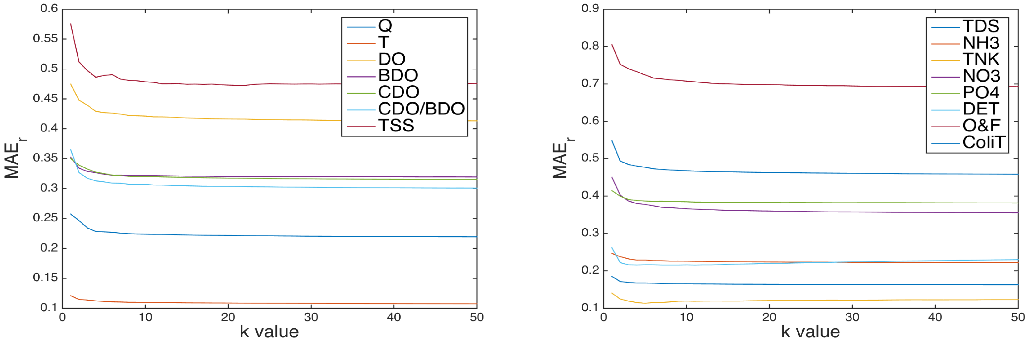
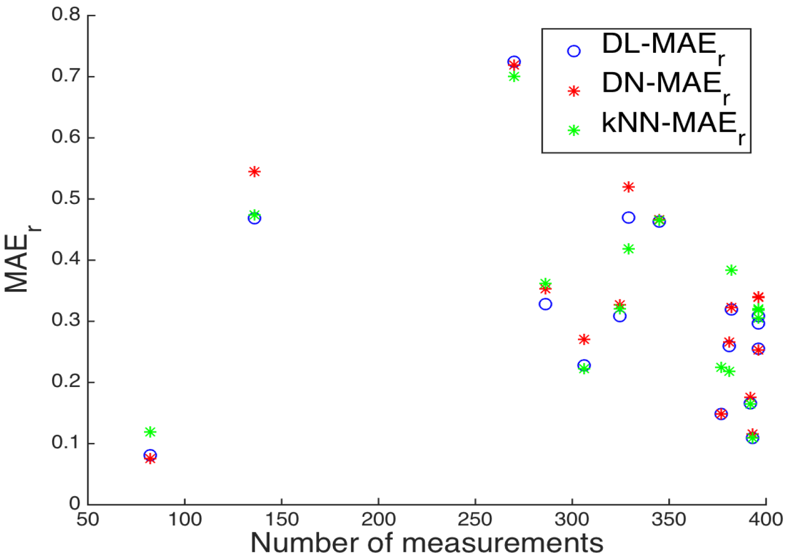
2.4. Behavior of Interpolation Errors

Given that the interpolation error depends on the analyzed variable, the number of measurements, and the interpolation method, it is advisable to use a relative error of the MAE value. Following [23], in this work, we use
M A E r = M A E u ,
where MAE r is the relative error of MAE, and u is the average value of each variable of water quality.
On the other hand, the MAE obtained by the kNN algorithm for different variables of water quality depends on the k parameter, which takes different values due to the nature of each variable.

3. Results

In this section, the performance of the interpolation algorithms is analyzed, based on data from monitoring campaigns conducted in irregular time periods and non-uniform distances between stations. This is a usual situation, which can be due to logistical problems or bad weather conditions, among other factors.

3.1. Free Parameter k and Algorithm Comparisons

In order to establish a comparison between deterministic and statistical interpolation, we started by scrutinizing the value of k to be used as a free parameter in the kNN algorithm. Figure 3 shows the changes of MAE r with respect to k. It can be observed that we almost always need few neighbors for yielding a value close to the minimum MAE. As errors decrease very slowly after some point, and for computational simplicity, we decided to use k = 15 for all the kNN variable models. On the other hand, Figure 4 shows the variability of MAE r with respect to the normalized number of measurements. It can be observed that MAE r is reduced by increasing the number of available samples, though a extremely reduced number of available samples sometimes can yield an apparently reduced error, probably due to the poor representation of the dynamics in these cases.
Table 3 presents the MAE of each variable obtained with each interpolation algorithm (with k = 15 for kNN). Note that MAE values are significantly different among water quality variables, and because of that, we also included the relative MAE (MAE r ). The average value of MAE r was 0.31 for Delaunay-linear, 0.33 for Delaunay-nearest, and 0.32 for kNN, which, roughly speaking, shows that about two thirds of the variations are jointly explained by the underlying dynamics.
We also analyzed which interpolation method provides with the best estimation of the dynamics (i.e., trends or patterns) for the observed variables. Figure 5a shows the interpolation of NH 3 with Delaunay-linear, which also resembles the one obtained by applying Delaunay-nearest shown in Figure 5b. Both interpolation techniques present a typical step-like view of the interpolated variable. On the other hand, Figure 5c shows the interpolation results of NH 3 with the kNN method. In this later case, data dynamics are better observed because of the improved smoothing, allowing us to easily see spatial and temporal trends. As another example, Figure 5d shows PO 4 interpolation with Delaunay-linear, while Figure 5e shows a noticeable smoothing when the kNN method is used. Again, the kNN technique shows more clearly some spatial trends for the PO 4 variable. Figure 5f shows another example of the ColiT interpolation when using the kNN method, displaying the dynamics of some trends and consistent peaks on it. Interpolation errors of each method on each variable are detailed in Table 3.
Figure 6a shows the rainfall in the study area during the period 2002–2007 recorded by a nearby weather station. This information is included for comparison of some of the water quality variables in the same figure. The variables in Figure 6 are Q, T, DO, BOD/COD, and TNK, whose representations are drawn in elevation view for better visual observation of their spatio-temporal dynamics. As far as Figure 5 and Figure 6 show eight variables of a total of 15 water quality parameters of Machángara River, the seven remaining variables that are not represented are BOD, COD, TDS, TSS, NO 3 , DET, and O&F. It should be noted that those representations exhibit a similar smoothing compared to the eight variables previously represented when using the kNN method.

3.2. Analysis of the Spatio-Temporal Model Residuals

In the previous section, it was not clear which interpolation method performed better just in terms of averaged error. For a fair benchmarking, we proposed making an analysis on the spatio-temporal distribution of the model residuals. Taking into account that the leave-one-out residual was obtained for each method in each sample, Figure 7 displays the difference in terms of Absolute Error ( A E ) between kNN and Delaunay methods for six different variables. Blue markers represent the difference of A E ( Δ A E = A E D e l a u n A E k N N ) when Delaunay obtains worse performances than kNN (i.e., for the case A E D e l a u n A E k N N > 0 ) and red markers are shown otherwise (i.e., for the case Δ A E = A E k N N A E D e l a u n ).
From Figure 7, several ideas can be summarized. Although the largest differences (due to outliers or atypical measurements) can be obtained for both methods in some cases, as seen in (e,f), outliers are better treated by kNN in most of the cases, as seen in (a–d). In addition, kNN works better for some given variables, which are (a,b), and (d), whereas its performance can degrade compared to Delaunay in cases such as (e), or it can be similar in cases such as (f).
If we compare these results with the observations and estimation in Figure 5, it can be concluded that kNN works better for outliers and for slow-dynamics variables with smooth changes, whereas fast-dynamics variables can be over-smoothed by this method, and, then its model residuals are not capable of improving the trivial interpolation made by Delaunay.

3.3. Evolution of Water Quality Measurements

Flow rate (Q). Figure 6b shows the Machángara River flow rate, and it depends on several factors, namely, the tributaries formed by streams coming from the Pichincha volcano (Quito is a city located between the slopes of a volcano and the Machángara River), the runoffs due to rainfall in the upper basin of Quito, and the wastewater from domestic and industrial discharges in the central and the southern parts of the city. Additionally, Quito does not have independent pipes for domestic, industrial, or runoff water, but rather this wastewater is a composition of all them. Figure 8 represents the average of the maximum values of flow rates for each year from 2002 to 2007 of a total of 19 major tributaries upstream of the Machángara River. Figure 8 shows two peaks ( m 3 / s ) that are present at about 500 days (2003) and 1250 days (2005), whereas we can see a decrease of the flow rate at 800 days (2004), likely due to the scarcity of rains. Although this represents an annually averaged measurements of flow rates, this plot and the rainfall one (Figure 6a) could better explain the evolution of water discharges into the river as shown in Figure 6b. In this last figure, two flow rate peak at about 500 and 1500 days are displayed, which could be due to rainfall and flow rate of the Machángara River’s tributaries. The changes in the total flow could affect the behavior of other water quality characteristics.
Dissolved Oxygen (DO). Figure 6c shows that DO increases in space after about 2 km, and in time especially after January 2006 (1460 days). Figure 6d shows a temperature increase in the river´s water at the last station (9.49 km). As temperature increases, oxygen solubility decreases. Therefore, dissolved oxygen should be lower (see Figure 6c). In addition, it can be observed that DO increases during the last 600 days between ST3 and ST5. In this section, the Machángara River has a lot of stones and debris. This condition may cause an intensive crush of water against these materials, hence producing a large amount of small water bubbles. It is well known that as water bubbles get smaller, the liquid–gas interface area increases, and thus oxygen can be dissolved at a higher rate. As a result, DO should be also higher. In addition, temperatures in the last 600 days in those stations showed a slight decrease which could also contribute to the increase of DO.
Temperature (T). Water temperature, shown in Figure 6d, is another relevant parameter in the study of the river water quality. It mainly depends on temperature of domestic and industrial discharges, rainfall, and environmental temperature. The spatio-temporal distribution shows two main effects, namely, an increase in the space after 8 km, and an increase after 6 km only present after 1750 days (October 2006). This temperature change in the last 300 days could be two-fold: (1) in general, the ambient temperature has increased in the last years due to the global warming effect, and the water of the Machángara River (shallow river) has also received the global impact increasing its temperature; and (2) population close to the river has also increased in that period of time. In fact, Quito’s population was 1,842,202 inhabitants in 2001, while it was 2,239,191 in 2010, a growth rate of 2.41% per year [24]. Thus, hot water for personal care, washing kitchen utensils, and cleaning activities in hospitals and industries are discharged in the river.
Biodegradability index (BOD/COD). Organic matter biodegradability can be estimated by the ratio between BOD and COD [25]. According to [26], the organic matter biodegradability is classified as follows:
  • If BOD/COD ≥ 0.4, then organic matter is very degradable.
  • If BOD/COD ∈ (0.2, 0.4), then organic matter is moderately degradable.
  • If BOD/COD ≤ 0.2, then organic matter is little degradable.
Figure 6e shows the BOD/COD ratio where there is a relatively stable value with distance. In the time period between 800 and 1200 days, there were several industries in the study area, which used to discharge a high amount of non-biodegradable liquid compounds. To investigate the pollution impact caused by their water discharges directly into the Machángara River in the time period of 2002 to 2007, there were taken into account a total of 54 representative industries of all cities upstream of the river, and there were two important industrial zones that had 15 industries (27.78%), mainly textiles (dyes) and food and beverage (dyes). The municipal authorities of Quito assessed industries that met wastewater treatment regulations before discharging them into river. Results showed that industries meeting water quality standards were 75% in 2005, 63% in 2006 and 69% in 2007. It is most likely that industries that did not meet environmental regulations contributed to a high load of non-biodegradable compounds discharged into the river. Unfortunately, there is no more information from the other years.
Total Nitrogen Kjeldahl (TNK). This variable is the sum of ammonia (NH 3 ) and ammonium (NH 4 + ), and the maximum allowed value in Ecuador is 40 mg/L according to [27]. Figure 6f shows the TKN variation, which is in this case constrained to about the last 400 days of measurements. In general, there is a sustained level near the limit, both below and above it, for most of the available monitored periods.

4. Discussion

Since topography is stable with time, it can be treated with deterministic interpolation (such as the Delaunay algorithm). However, water dynamics can not be determined accurately by just deterministic interpolation, except for simple visualization purposes. Our work shows that statistical interpolation is capable of estimating the water dynamics with moderate model orders and distinguishing between dynamics, given by the spatio-temporal trends present in the model, and perturbations of a very different nature, given by the model residuals (including system perturbations, measurement errors, outliers and atypical values, and other uncertainty sources). Despite the main relevance of system knowledge to improve the water quality, our motivation for this work has been given by the idea that current system knowledge is partly guided by measurements. In addition, spatio-temporal statistical interpolation of measurements can enhance the information that can be extracted from the data for helping to improve the knowledge on the sources of pollution.
In many previous works, (i.e, [10,13]) databases built in no longer than two years were used. Alternatively, in this work, we used a five-year monitoring database, which allowed for a significant amount of records of water quality parameters similar to the work described in [11,28]. Our database consisted of 64 monitoring campaigns and 4867 water quality records. This allowed us to build interpolation grids with a spatial resolution of 400 m and a temporal resolution of one day. We obtained a simple to adjust k value by using the kNN algorithm where a stable and close to minimum MAE was achieved. This simplicity allowed us to construct a spatio-temporal grid with the measured water quality parameters and the data processed by nonuniform interpolation methods.
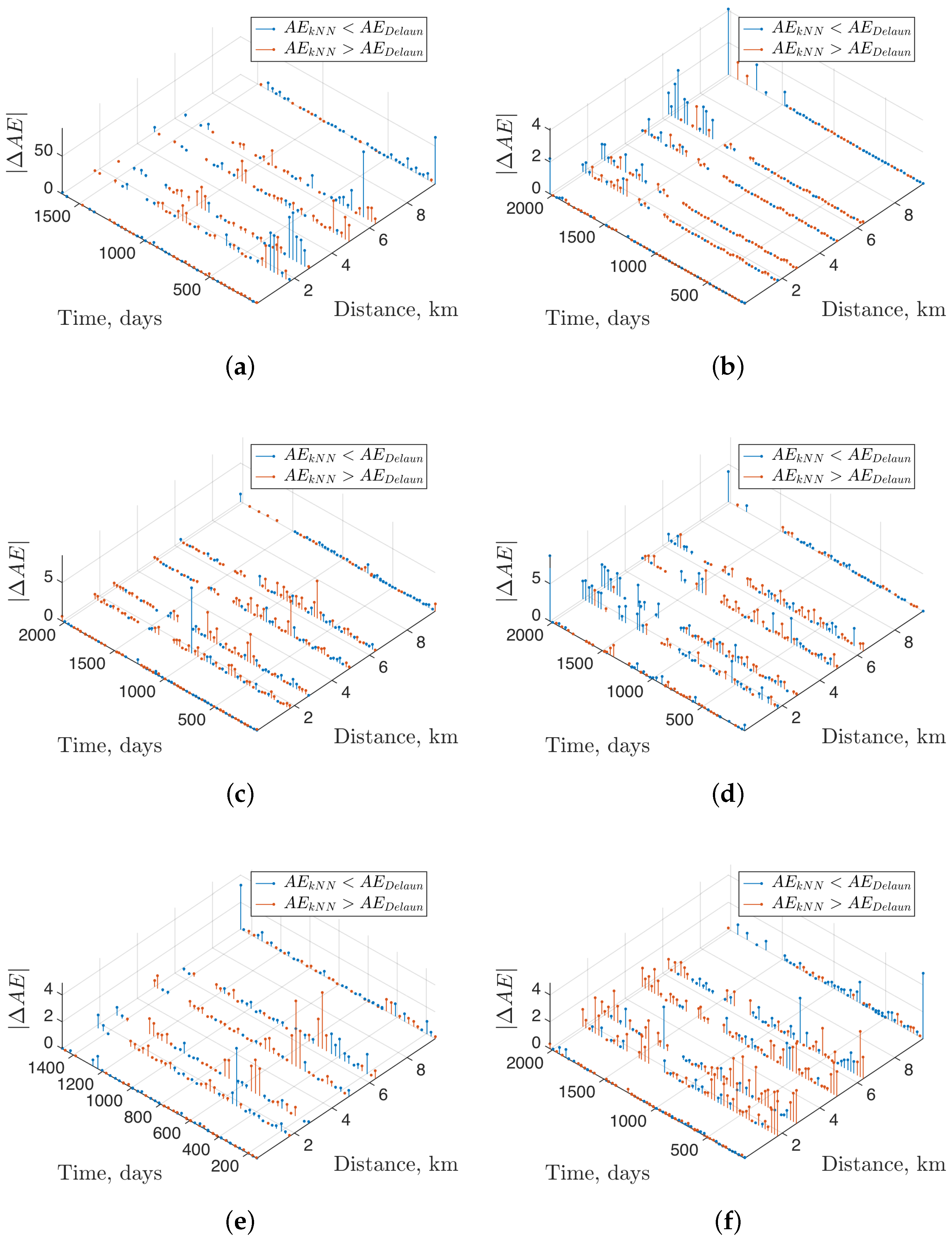
When analyzing the model residuals for comparison between kNN and Delaunay interpolation, we found that kNN estimation provides acceptable estimation of the variable dynamics in the presence of atypical samples, and in slow-dynamics variables, whereas it can present some over-smoothing effects on fast-changing variables. This suggests that, whereas conventional interpolation algorithms can provide acceptable estimation capabilities, further interpolation algorithms should be designed for overcoming their current limitations.
The MAE obtained for phosphates in [11] was 0.466 by using Bayesian methods, while, in this work, it is 1.08 when using kNN. This difference could be due to different water quality datasets, and, therefore, it does not stand for a straight comparison. However, we consider this previous work as comparable to ours in terms of estimation techniques. While [29] presents only the nitrate dynamics of the Turia River (Valencia Spain), in this paper we show nitrogen and other variables with good spatio-temporal resolution.

5. Conclusions

The proposed spatio-temporal analysis of water quality measurements using interpolation algorithms for measurements from campaigns can provide useful and relevant information on their dynamics, in the sense of trends and structure. This can complement the current knowledge from the experience and from physical models and help extend it. New methods of interpolation are encouraged to overcome the limitations of conventional interpolation methods in this scenario. While a secondary target, visualization of these trends provides a way of visually inspecting the data models, and residual visualization can provide data quality measurement of the estimation model under use and its uncertainty.
Water quality values resulting from the application of the smoothing interpolation algorithms, especially for those places that are difficult to reach and for irregular time periods, can also provide relevant information for designers of wastewater treatment plants. For example, it can be used for other sections of the Machángara River and make studies about inter-dependence between water quality variables, (e.g., nitrates and phosphates).
The database used in this work corresponds to a period between 2002 and 2007, a time period when few hydrology monitoring stations existed for capturing the rainfall in the city or near the study zone. Even today, there are no more water quality monitoring stations than those ones constructed in 2002–2007. The major contributors of wastewater in the Machángara River are domestic and industrial discharge, and furthermore, in our city, there were no separate pipes for rainfall and wastewater (and still today there are not yet any). For these reasons, in our study, we especially missed having denser spatial sampling rates (stations), as well as the always desirable increase in time sampling rates (measurement campaigns).
A limitation of this study is the lack of time records (the hour of the day) in which the water samples were collected and analyzed. Variables such as water temperature, concentrations of detergents, phosphates, oils and fats are not constant during the 24 h, since they depend on discharge of domestic and industrial wastewater and meteorological conditions. Therefore, conducting an extended study considering smaller time periods between samples for 24 h each day could provide us with useful information for studies on the uses of water than could be characterized by time and population type.

Acknowledgments

This work was supported in part by the Universidad de las Fuerzas Armadas ESPE under Grant 2015-PIC-004 and has also been partly supported by Research Grants PRINCIPIAS (TEC2013-48439-C4-1-R) and FINALE (TEC2016-75161-C2-1-R) from the Spanish Government and PRICAM (S2013/ICE-2933) from Comunidad de Madrid. The authors thank the Metropolitan Water Company of Quito, Ecuador, for providing the Machángara River water quality data.

Author Contributions

Iván P. Vizcaíno, Enrique V. Carrera, José Luis Rojo-Álvarez and Luis H. Cumbal conceived and designed the experiments. Iván P. Vizcaíno, Sergio Muñoz-Romero and Margarita Sanromán-Junquera performed the experiments. Enrique V. Carrera, Luis H. Cumbal and José Luis Rojo-Álvarez supervised the experiments. Iván P. Vizcaíno wrote the paper, and all authors contributed with changes in all sections.

Conflicts of Interest

The authors declare no conflicts of interest.

References

  1. Van der Perk, M. Soild and Water Contamination from Molecular to Catchment Scale, 1st ed.; Taylor and Francis/Balkema: Leiden, The Netherlands, 2006. [Google Scholar]
  2. Duan, W.; Takara, K.; He, B.; Luo, P.; Nover, D.; Yamashiki, Y. Spatial and temporal trends in estimates of nutrient and suspended sediment loads in the Ishikari River, Japan, 1985 to 2010. Sci. Total Environ. 2013, 461–462, 499–508. [Google Scholar] [CrossRef] [PubMed]
  3. Duan, W.; He, B.; Takara, K.; Luo, P.; Nover, D.; Sahu, N.; Yamashiki, Y. Spatiotemporal evaluation of water quality incidents in Japan between 1996 and 2007. Chemosphere 2013, 93, 946–953. [Google Scholar] [CrossRef] [PubMed]
  4. Heinke, G.G. Ingeniería Ambiental, 2nd ed.; Prentice Hall Hispanoamericana, S.A.: Upper Saddle River, NJ, USA, 1999; pp. 421–424. [Google Scholar]
  5. Tebbutt, T.H.Y. Principles of Water Quality Control, 5th ed.; Butterworth-Heinemann an Imprint of Elsevier Science: Oxford, UK, 1998; pp. 21–22. [Google Scholar]
  6. Corcoran, E.; Nellemann, C.; Baker, E.; Bos, R.; Osborn, D. Sick Water? The Central Role of Wastewater Management in Sustainable Development; Savelli, H., Ed.; Birkeland Trykkeri AS: Birkeland, Norway, 2010. [Google Scholar]
  7. Meneses, M.; Concepción, H.; Vilanova, R. Joint Environmental and Economical Analysis of Wastewater Treatment Plants Control Strategies: A Benchmark Scenario Analysis. Sustainability 2016, 8, 360. [Google Scholar] [CrossRef]
  8. Thangarajan, M. Groundwater Resource Evaluation, Augmentation, Contamination, Restoration, Modeling and Management; Springer: Dordrecht, The Netherlands; Capital Publishing Company: New Delhi, India, 2007; pp. 12–17. [Google Scholar]
  9. Taalohi, M.; Tabatabaee, H. Predicting Bar Dam Water Quality using Neural-Fuzzy Inference System. Indian J. Fundam. Appl. Life Sci. 2014, 4, 630–636. [Google Scholar]
  10. Li, S.; Liu, W.; Gu, S.; Cheng, X.; Xu, Z.; Zhang, Q. Spatio temporal dynamic of nutrients in the upper Han River basin, China. Hazard. Mater. 2009, 162, 1340–1346. [Google Scholar] [CrossRef] [PubMed]
  11. Serre, M.; Carter, G.; Money, E. Geostatistical space/time estimation of water quality along the Raritan river basin in New Jersey. Dev. Water Sci. 2004, 55, 1839–1852. [Google Scholar]
  12. Duan, W.; He, B.; Nover, D.; Yang, G.; Chen, W.; Meng, H.; Zou, S.; Liu, C. Water Quality Assessment and Pollution Source Identification of the Eastern Poyang Lake Basin Using Multivariate Statistical Methods. Sustainability 2016, 8, 133. [Google Scholar] [CrossRef]
  13. Gomez, M.; Herrera, S.; Solé, D.; García-Calvo, E.; Fernández-Alba, A. Spatio temporal evaluation of organic contaminants and their transformation products along a river basin affected by urban, agricultural and industrial pollution. Sci. Total Environ. 2012, 420, 134–145. [Google Scholar] [CrossRef] [PubMed]
  14. Empresa Pública Metropolitana de Agua Potable Quito. Estudios de Factibilidad y Diseños Definitivos del Plan de Descontaminación de los Ríos de Quito Informe No.1 “Revisión de la Información Existente y Diagnóstico”; Technical Report; Empresa Pública Metropolitana de Agua Potable Quito: Quito, Ecuador, 2009.
  15. Municipio del Distrito Metropolitano de Quito. Plan de Desarrollo 2012–2022. Consejo Metropolitano de Planificación. Quito, Ecuador; Municipio del Distrito Metropolitano de Quito: Quito, Ecuador, 2011; pp. 14–26.
  16. Priego de los Santos, J.; Porres de la Haza, M. La Triangulación Delaunay Aplicada a los Modelos Digitales del Terreno; Universidad Politécnica de Valencia: Valencia, Spain, 2002; pp. 1–8. [Google Scholar]
  17. De-Berg, M.; Cheong, O.; Van-Kreveld, M.; Overmars, M. Computational Geometry, Algorithms and Applications, 3rd ed.; Springer: Berlin/Heidelberg, Germany, 2008; pp. 196–198. [Google Scholar]
  18. Karl, S.; Truong, Q. An Adaptable k-Nearest Neighbors Algorithm for MMSE Image Interpolation. IEEE Trans. Image Process. 2009, 18, 1976–1987. [Google Scholar]
  19. Cherkassky, V.; Mulier, F. Learning From Data: Concepts, Theory, and Methods, 2nd ed.; Wiley-Interscience: Hoboken, NJ, USA, 2007; pp. 61–64. [Google Scholar]
  20. Elisseeff, A.; Pontil, M. Leave-one-out error and stability of learning algorithms with applications. Mach. Learn. Res. 2002, 55, 71–97. [Google Scholar]
  21. Mukherjee, S.; Niyogi, P.; Poggio, T.; Rifkin, R. Statistical Learning: Stability Is Sufficient For Generalization and Necessary and Sufficient for Consistency of Empirical Risk Minimization; Massachusetts Institute of Technology: Cambridge, MA, USA, 2004. [Google Scholar]
  22. Rogers, S.; Girolami, M. A First Course in Machine Learning, 1st ed.; Chapman & Hall/CRC: New York, NY, USA, 2011; pp. 29–31. [Google Scholar]
  23. Uriel-Jiménez, E.; Aldás-Manzano, J. Análisis Multivariante Aplicado; Thomson Editores Spain Paraninfo S.A.: Madrid, Spain, 2005; pp. 56–57. [Google Scholar]
  24. Instituto Nacional de Estadísticas y Censos. Base de Datos Censo 2010; INEC: Quito, Ecuador, 2010.
  25. Tien, M.; Lai, J.; Jin, H. Estimating the Biodegradability of Treated Sewage Samples Using Synchronous Fluorescence Spectra. Sensors 2011, 11, 7382–7394. [Google Scholar]
  26. Martín, I.; Betancourt, J. Guía Sobre Tratamientos de Aguas Residuales Urbanas para PequeñOs NúCleos de PoblacióN. Mejora de la Calidad de los Efluentes, 1st ed.; Daute Diseño, S.L.: Las Palmas, Spain, 2006. [Google Scholar]
  27. Presidencia de la República del Ecuador. Norma de Calidad Ambiental y de Descarga de Efluentes: Recurso Agua; Technical Report; Presidencia de la República del Ecuador: Quito, Ecuador, 2012.
  28. Clement, L.; Thas, O.; Vanrolleghem, P.A.; Ottoy, J.P. Spatio-temporal statistical models for river monitoring networks. Water Sci. Technol. 2006, 53, 9–15. [Google Scholar] [CrossRef] [PubMed]
  29. Capella, J.; Bonastre, A.; Ors, R.; Peris, M. In line river monitoring of nitrate concentration by means of a Wireless Sensor Network with energy harvesting. Sens. Actuators 2013, 177, 419–427. [Google Scholar] [CrossRef]
Figure 1. Monitoring station location at the Machángara River. The station name and numeric codes were provided by the Metropolitan Water Company of Quito, Ecuador.
Water 08 00507 g001
Figure 2. Representation and nomenclature of the elements in our Delaunay interpolation: (a) Delaunay triangulation and Voronoi diagram; and (b) obtaining a polyhedral from a set of sample points.
Water 08 00507 g002
Figure 3. Behavior of MAE r for different k values.
Water 08 00507 g003
Figure 4. MAE r for different normalized numbers of measurements. DL-MAE r is for Delaunay linear, DN-MAE r is for Delaunay nearest, and kNN-MAE r is for kNN method.
Water 08 00507 g004
Figure 5. Results of Delaunay and kNN Interpolation methods: (a) NH 3 with Delaunay linear; (b) NH 3 with Delaunay nearest; (c) NH 3 with kNN; (d) PO 4 with Delaunay linear; (e) PO 4 with kNN; and (f) ColiT with kNN.
Water 08 00507 g005aWater 08 00507 g005b
Figure 6. Spatio-temporal variation: (a) rainfall level in Quito from 2002 to 2007 at `La Tola’ monitoring station; (b) Q; (c) DO; (d) T; (e) BOD/COD; (f) TNK.
Water 08 00507 g006
Figure 7. Spatio-temporal distributions for | Δ A E | = | A E k N N A E D e l a u n | : (a) O&F; (b) DET; (c) BOD/COD; (d) DO; (e) NO 3 ; and (f) PO 4 .
Water 08 00507 g007
Figure 8. Average of the maximum values of flow rates for each year (from 2002 to 2007) depicted when time is shown in days.
Water 08 00507 g008
Table 1. Monitoring Stations of Machángara River. ST1 is the first station and d is the distance from each station with respect to the first one. Each monitoring station name is followed by the original code provided by the Metropolitan Water Company of Quito, Ecuador.
Station NameCoded (km)
R. Mch. El Recreo (2.07)ST10.00
R. Mch. Villaflora (2.08)ST21.75
R. Mch. El Sena (2.09)ST32.75
R. Mch. El Trébol (2.10)ST44.91
R. Mch. Las Orquídeas (2.11)ST56.31
Q. El Batán (1.09)ST69.49
Table 2. Studied water quality parameters for the case study of the Machángara River.
VariableAcronymUnits
Flow rateQm 3 /s
TemperatureT C
Dissolved OxygenDOmg/L
Biochemical Oxygen DemandBODmg/L
Chemical Oxygen DemandCODmg/L
BOD/COD ratioBOD/COD
Total Dissolved SolidsTDSmg/L
Total Suspended SolidsTSSmg/L
AmmoniaNH 3 mg/L
Total NitrogenTNKmg/L
NitrateNO 3 mg/L
PhosphatesPO 4 mg/L
DetergentsDETmg/L
Oils and FatsO&Fmg/L
Total Escherichia coliColiTmg/L
Table 3. Interpolation errors for each variable with nonuniform interpolation methods.
VariableNo.MAEMAErMAEMAErMAEMAEr
Measur.(Dela_lin)(Dela_lin)(Dela_nea)(Dela_nea)(k = 15)(k = 15)
Q3060.600.230.710.270.580.22
T3931.880.112.000.121.880.11
DO3291.160.471.280.521.030.42
BOD39647.240.3152.140.3449.140.32
COD396106.990.30122.360.34114.960.32
BOD/COD3960.660.250.650.250.790.30
TSS136122.540.47142.420.55123.940.47
TDS39251.180.1754.340.1850.930.16
NH 3 3773.090.153.080.154.660.22
TNK822.900.082.700.084.250.12
NO 3 2860.590.330.630.350.650.36
PO 4 3820.900.320.910.321.080.38
DET3810.270.260.270.270.220.22
O&F27010.710.7210.640.7210.370.70
ColiT3451.530.461.540.471.540.46
Average324 0.31 0.33 0.32
Note: Mean Absolute Error (MAE) and relative error of MAE (MAEr) for Delaunay linear (Dela_lin), Delaunay nearest (Dela_nea) and k-Nearest Neighbors (kNN) methods.

