Article

Rainfall Characteristics and Regionalization in Peninsular Malaysia Based on a High Resolution Gridded Data Set

1
Faculty of Civil Engineering, Universiti Teknologi Malaysia, Johor Bahru 81310, Malaysia
2
Department of Irrigation and Drainage, Jalan Sultan Salahuddin, Kuala Lumpur 50626, Malaysia
3
School of Environment and Natural Resource Sciences, Universiti Kebangsaan Malaysia, Bangi 43600, Malaysia
4
Centre for Environmental Sustainability and Water Security, Research Institute for Sustainable Environment, Universiti Teknologi Malaysia, Johor Bahru 81310, Malaysia
5
UNESCO-IHE Institute for Water Education, Westvest 7, Delft 2611 AX, The Netherlands
6
World Water Assessment Programme (WWAP), UNESCO Villa La Colombella—Località di Colombella Alta, Perugia 06134, Italy
*
Authors to whom correspondence should be addressed.
Water 2016, 8(11), 500; https://doi.org/10.3390/w8110500
Submission received: 14 September 2016 / Revised: 18 October 2016 / Accepted: 25 October 2016 / Published: 2 November 2016
(This article belongs to the Special Issue Advances in Hydro-Meteorological Monitoring)

Abstract

:
Daily gridded rainfall data over Peninsular Malaysia are delineated using an objective clustering algorithm, with the objective of classifying rainfall grids into groups of homogeneous regions based on the similarity of the rainfall annual cycles. It has been demonstrated that Peninsular Malaysia can be statistically delineated into eight distinct rainfall regions. This delineation is closely associated with the topographic and geographic characteristics. The variation of rainfall over the Peninsula is generally characterized by bimodal variations with two peaks, i.e., a primary peak occurring during the autumn transitional period and a secondary peak during the spring transitional period. The east coast zones, however, showed a single peak during the northeast monsoon (NEM). The influence of NEM is stronger compared to the southwest monsoon (SWM). Significantly increasing rainfall trends at 95% confidence level are not observed in all regions during the NEM, with exception of northwest zone (R1) and coastal band of west coast interior region (R3). During SWM, most areas have become drier over the last three decades. The study identifies higher variation of mean monthly rainfall over the east coast regions, but spatially, the rainfall is uniformly distributed. For the southwestern coast and west coast regions, a larger range of coefficients of variation is mostly obtained during the NEM, and to a smaller extent during the SWM. The inland region received least rainfall in February, but showed the largest spatial variation. The relationship between rainfall and the El Niño Southern Oscillation (ENSO) was examined based on the Multivariate ENSO Index (MEI). Although the concurrent relationships between rainfall in the different regions and ENSO are generally weak with negative correlations, the rainfall shows stronger positive correlation with preceding ENSO signals with a time lag of four to eight months.

1. Introduction

Delineating climatic zones facilitates the investigation of the general climate characteristics of the region, and helps improve understanding of climate variability across a range of spatial and temporal scales. It plays an important role in gaining knowledge of water balance dynamics on various scales for water resources planning and management [1,2,3]. At low latitudes, where temperatures vary little within and over years, climate differences are largely determined by differences in rainfall patterns. Climatic boundaries are often plotted according to mean monthly rainfall, varying gradually except where the gradients steepen on mountain slopes or along seacoasts [4]. Distinction between zones is always arbitrary and relies on the cartographical convenience. For example, the climatic regions are grouped according to the same category of isohyet range, the climatic zones boundaries are not clear and are always subjectively determined [4]. Thus, an objective quantitative climatic classification is essential for discovering definite and distinctive climate zones boundaries using the climatic data.
The relationship between monsoon seasons and rainfall of Peninsular Malaysia was studied by Lim [5]. He delineated rainfall regions based on 29 rainfall stations and assessed pentad rainfall patterns that could be grouped roughly into five rainfall regions. These results became the reference for the researchers in investigating rainfall distribution across the country [6,7,8,9]. Bishop [10] who researched on integration of land use and climatic data, believed that this could produce good region classification. However, his efforts generated some doubts over certain regions, which were mainly attributed to the reliability of climatic data used in his research. He recommended that a more sophisticated statistical analysis procedure and better data sets be applied to overcome the uncertainty in defining the climatic regions.
With the defined climatic regions, the knowledge of past rainfall distribution and patterns can be assessed in order to qualify the nature of changes in time and space. In the past, most of the hydroclimatic studies focused on rainfall distribution and patterns of change over time. For example, Nieuwolt [11] adopted an agricultural rainfall index to quantify rainfall variability over time. Researchers further investigated the temporal and spatial characteristics of rainfall during 1990s, but often restricted their analyses to small catchments, e.g., an urbanized area [12] or a forested catchment [13].
Peninsular Malaysia has undergone development at a rapid pace over last decades. Thus, the overall picture of country water resources distribution has become important for future water resources planning and management. However, a comprehensive regional study of rainfall patterns is still very limited. The mean annual rainfall maps, derived from long-term monthly records (1950–1990) by the Economic Planning Unit [14,15], are only able to show the spatial distribution of average rainfall in the country instead of high temporal and spatial variability of rainfall patterns. Regional trends of rainfall distribution also have not received much attention from researchers.
The climate over Peninsular Malaysia is subjected to pronounced interannual variability which modulates hydrological variability, including floods and droughts [16,17,18]. The relation between Malaysian rainfall anomalies, sea surface temperature and El Niño-Southern Oscillation (ENSO) were studied by Tangang and Juneng [17] and Juneng and Tangang [19,20]. The global warming/temperature trends and variations were investigated by Tangang et al. [21] and Ng et al. [22]. However, these studies were based solely on station observations which have insufficient spatial coverage [23], biases associated with the gauge measurement process and homogeneity of rainfall time series [24], and problems of missing data [23]. The need for data with better accuracy and space-time resolution has been emphasized by many researchers [12,25,26,27].
The development of gridded rainfall data sets [27] can provide better spatio-temporal coverage across a region. It is also timely to reassess the climatic regions as defined by Lim [5] and Bishop [10], and investigate regional rainfall trends and distribution to update the understanding of the spatial and temporal variability in the country and support further water resource planning and management.
The aim of this study is two-fold. First, to delineate climatic regions using clustering algorithm based on the daily gridded rainfall data set for Peninsular Malaysia. Second, to explore the regional characteristics of rainfall distribution through trend analysis and analysis of spatial rainfall variability on annual and monsoon-seasonal basis for different climatic regions.

2. Materials and Methods

2.1. Study Area

Peninsular Malaysia is located in the tropics between 1° and 7° north and between 99° and 105° east. The total area of 132,000 km2 is composed of highlands, floodplains and coastal zones. The Titiwangsa range forms the backbone of the Peninsula, running approximately south-southeast from southern Thailand over a distance of 480 km and separating the eastern part from the western part. Surrounding the central high regions are the coastal lowlands. In general, the Peninsula experiences a warm and humid tropical climate all year round, with uniform temperatures ranging from 25 °C to 32 °C. Rainfall is characterized by two rainy seasons associated with the southwest monsoon (SWM) from May to September and the northeast monsoon (NEM) from November to March [7,16,28].

2.2. Data Sources

The rainfall data used in this study is the gridded data set described by Wong et al. [27] for a period of 31 years from 1976 to 2006. The daily rainfall data originates from four data sources, i.e., the automatic station database of the Department of Irrigation and Drainage (DID), the Malaysian Meteorological Department (MMD), the Global Summary of the Day (GSOD) that archived at the National Climatic Data Center of the National Oceanic and Atmospheric Administration (NOAA/NCDC) was transmitted over the Global Telecommunication System of the World Meteorological Organisation (WMO-GTS), and additional Global Energy and Water Balance Experiment (GEWEX) research programme Asian Monsoon Experiment (GAME) data which also originate from MMD. The combination of all data sources brings an average of 123 daily point observations with maxima of 167 in years 2001 and 2003.

2.3. Methodology

Rainfall regions are delineated from annual rainfall cycles based on monthly climatological values using a clustering algorithm. The delineated regions were then analyzed statistically to assess the spatio-temporal rainfall distribution. Rainfall trends were investigated using Mann-Kendall nonparametric trend detection method. The spatial variability of annual and monsoon rainfall of all regions is calculated. The relationship and influence of El Ninõ-Southern Oscillation (ENSO) over the delineated regions is assessed by using the Multivariate ENSO Index (MEI) indicator.

2.3.1. Data Interpolation

The rainfall is interpolated directly from point observation values. The input data stations are mostly located at elevations below 300 m above sea level (m.a.s.l) with relatively few stations at higher altitudes between 1000 and 2000 m.a.s.l. Analysis of the available data did not reveal a clearly identifiable orographic relationship in daily rainfall between the station time series. The available rainfall data have been interpolated into daily grids with 0.05 degree resolution (approximately 5.5 km). The interpolation scheme is based on an adaption of Shepard’s [29] angular distance weighting (ADW) procedure.

2.3.2. Climatic Regions Delineation

Zones of different annual rainfall cycles based on monthly climatological values were identified using a clustering algorithm. The identification of groups or clusters is based on the similarity between data properties. There are several algorithms developed for this purpose. Here, a non-hierarchical K-means clustering algorithm [30] coupled to an empirical orthogonal function (EOF) analysis was applied.
There are 4289 rainfall grid cells in the study areas. Hence, the size of monthly rainfall climatological data matrix is 4289 × 12. In order to reduce the dimensionality of the data and to filter the random noise, the EOF analysis [31] was applied to the monthly rainfall climatological matrix. The EOF analysis is also commonly known as principal component analysis (PCA) in statistical literature [32]. A Monte-Carlo randomization test suggests a cut-off point at the sixth principal component which describes a total of ~98% of the cumulative variance in the data matrix. The resulting data matrix (4289 × 6) was subjected to the non-hierarchical K-means clustering algorithm.
The K-means clustering algorithm minimizes the Euclidean distance between the data items and the cluster centroid by partitioning the data into k non-overlapping regions. Each of the data items is represented by six values corresponding to the six principal components selected earlier. The algorithm iteratively minimizes the total intra-cluster variance (V) described by the following:
V = i = 1 k x j C i ( x j μ i ) 2
where Ci shows the ith cluster (i = 1, 2, …, k) and μi is the centroid of all the cluster points x j C i . The algorithm however requires the number of clusters, k, to be set a priori. Here, the algorithm was applied to the 4289 data items, setting the value of k from 3 to 10. The validity of the optimum number of cluster was then determined by the silhouette width [33] for each data items is calculated as:
S ( i ) = b ( i ) a ( i ) max { a ( i ) , b ( i ) }
where a(i) is the averaged Euclidean distance of the i data item to all other data items in the same cluster, b(i) is the minimum of the averaged distance of i data item to all data items in the other clusters. The averaged silhouette width, S ¯ evaluates the quality of the clustering solution by considering both compactness (distance between data items within the same cluster) and separation (distance between data items in two neighboring clusters). The closer S ¯ value is to 1, the better the grouping.

2.3.3. Trend Detection

The annual and monsoon seasonal averaged time series of rainfall of the climatic regions were analyzed using the Mann-Kendall nonparametric trend detection test [34,35]. The Mann-Kendall method has been widely used and tested to be an effective method to evaluate the presence of a statistically significant trend in climatological and hydrological time series [2,36,37,38]. In the trend test, the null hypothesis H0 is that there is no trend in the series (the data are independent and identically distributed). The alternative hypothesis H1 is that a trend exists in the data. The Kendall S-statistic is obtained from comparison between all possible (x, y) pairs of data and is given by:
S = i = 1 n 1 j = i + 1 n sgn ( x i x j ) sgn ( y i y j )
where, the sign function is defined (for any variable u) as
sgn ( u ) = { 1   if   u < 0       0   if   u = 0 + 1   if   u > 0
Under the null hypothesis, the statistic S is approximately normally distributed with zero mean and variance given by
Var ( S ) = n ( n 1 ) ( 2 n + 5 ) i = 1 n t i i ( i 1 ) ( 2 i + 5 ) 18
where ti is the number of ties of extent i in either the x or y data. The summation term in the numerator is used only if the data series contains tied values. The standardized test statistic Z is obtained as
Z = { S + 1   Var ( S ) if   S < 0 0 if   S = 0 S 1   Var ( S ) if   S > 0
The test statistic Z is used to measure the significance of a trend. In a two sided test, H0 should be accepted if |Z| is greater than Zα/2, where α represents the chosen significance level (e.g., 5% with Z0.025 = 1.96) then the null hypothesis is rejected implying that the trend is significant. A positive Z value indicates an upward trend, whereas a negative Z value indicates a downward trend. If a significant trend is present, the average rate of increase or decrease can be obtained from the slope of a simple linear regression.

2.3.4. Spatial Variation of Rainfall

Assessment of spatial variation is based on computation of the spatial variance within a particular delineated gridded region, as
σ 2 = 1 n i = 1 n ( x i x ¯ ) 2
where x ¯ is the average areal rainfall and, xi is the rainfall depth in each grid cell. The average areal rainfall and the spatial variance are computed for each region. The coefficient of variation of rainfall which is used to characterize the monthly spatial variability of rainfall is defined as the standard deviation divided by the average areal rainfall.

2.3.5. Rainfalls Correlation Analysis with El Ninõ-Southern Oscillation (ENSO)

The influence of ENSO over the delineated regions in Peninsular Malaysia is assessed by correlating the rainfall time series with the Multivariate ENSO Index (MEI). The MEI is based on six observed variables over the tropical Pacific Ocean, i.e., sea-level pressure, zonal and meridional components of the surface wind, sea surface temperature, surface air temperature, and total cloudiness fraction of the sky [39]. Negative values of the MEI represent the cold ENSO phase, i.e., La Niña, while positive MEI values represent the warm ENSO phase (El Niño). This index was chosen because it is less vulnerable to errors compared to station-based or single variable field based indices (e.g., Southern Oscillation Index, SOI) and has more robust key features in spatial variations and seasonal cycle [39].
To examine the relationship between the interannual rainfall and ENSO, each regional monthly rainfall index is correlated with the MEI time series concurrently. To further explore potential lagged influence of ENSO on NEM and SWM rainfall, the monsoon seasonal rainfall index is created to allow for comparison with the monthly MEI values preceding the seasons. The lag is defined by the time distance between the first month of monsoon season and monthly MEI value. For example, the correlation between the NEM rainfall and MEI at one month lag is the correlation coefficient value between the NEM, which is aggregated from November(0) to March(1)) rainfall and MEI value in October(0). The lagged correlation coefficient values were calculated with a lag time of 0–8 months (MEI leads the rainfall) as well as each individual monsoon month considered.

3. Results and Discussion

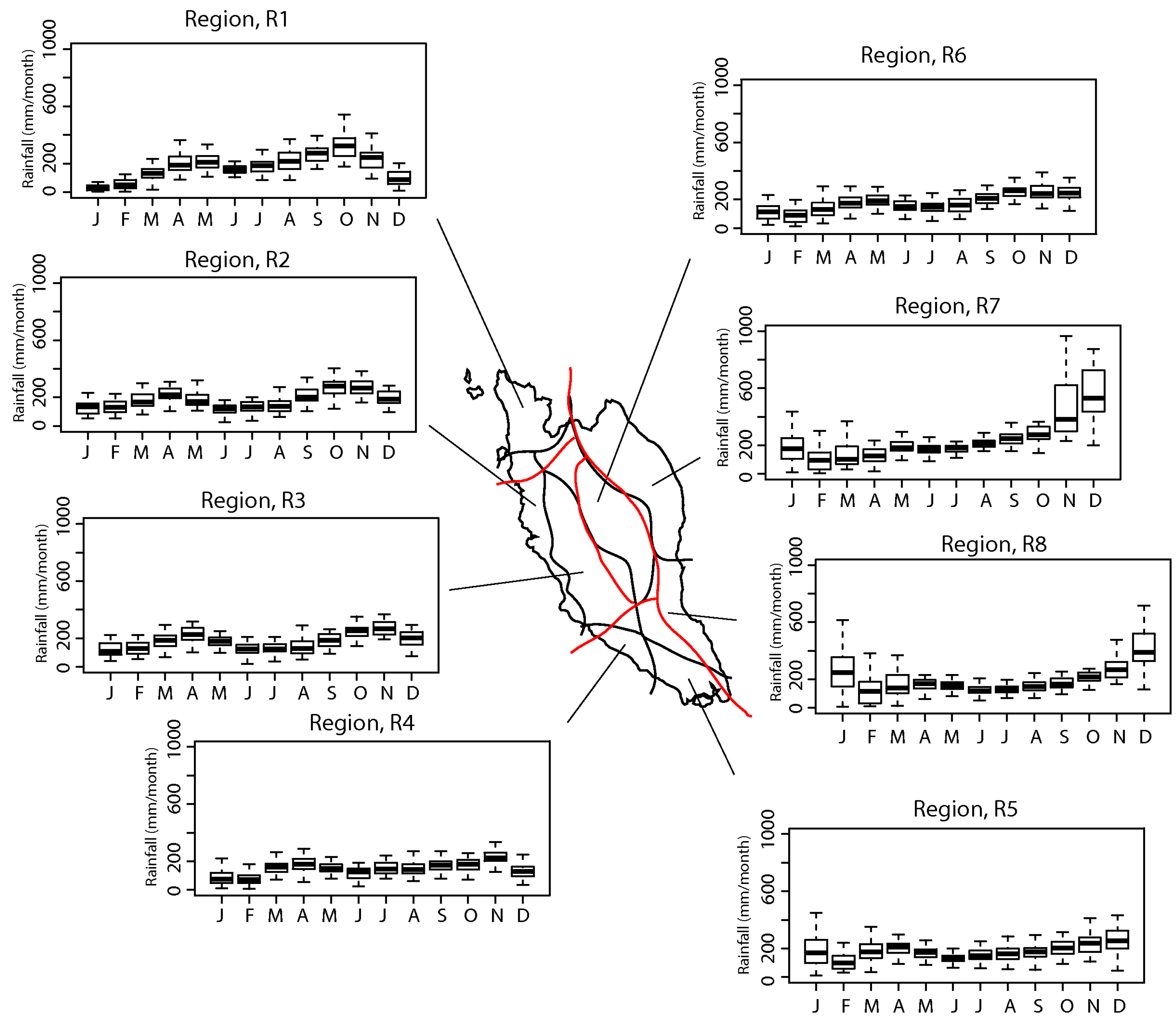
3.1. Characteristics of Delineated Climatic Regions

Table 1 shows the averaged silhouette width, S ¯ suggesting a best grouping of eight different regions for a maximum S ¯ value of 0.53. The eight delineated rainfall zones are shown in Figure 1. The classification patterns are generally consistent with Lim [5] that classified subjectively the Peninsular Malaysia rainfall into five different zones based on pentad data. The general similarity appears to be the existence of the northwest zone and the central interior rainfall zone over the central mountainous valley areas of Peninsular Malaysia. However, there exist some differences over the southern part of Peninsular Malaysia where current clustering algorithm further delineates the southwest zone of Lim [5] into two different rainfall zones. This rainfall characteristic is also observed by Dale [40] who reported the existence of a distinctive Port Dickson-Muar coastal rain belt in conjunction with other four larger rainfall zones. In addition, the east coast zone is further divided north-south into the northeastern zone and southeastern zone. The latter covers a large part of Johor state. Another difference between the current analysis and that of Lim [5] is the east-west separation of the west coast zone which is represented by region R6 (refer to Figure 1).
An examination of the rainfall zonation patterns and the regional topographic structure suggests that the delineation is closely associated with the topographic characteristics. The temporal variation of rainfall over Peninsular Malaysia is generally characterized by a bimodal annual cycle, i.e., a primary peak occurring during the autumn transitional period and a secondary peak during the spring transitional period as shown in Figure 1. However, over the east coast regions (R7), the rainfall appears to have a single peak during the NEM. This region received 2940 mm/year of mean annual rainfall, 52% and 33% of which occurred during NEM and SWM periods, respectively, as shown in Table 2. The monsoons contribute 85% of the total annual rainfall in this region. During the NEM, the dry northeasterly cold surge winds become moist during the passage over the South China Sea. The interaction with the land along the east coast area creates deep convection clouds and rainfall during the NEM [41,42,43]. The difference between the northeast zone (R7) and southeast zone (R8) appears to be the higher monsoon rainfall during November–December over the northeastern coast region (see Figure 1). Based on numerical experiments, Juneng et al. [43] argued that the higher elevation in the interior parts of the north-eastern coast of Peninsular Malaysia (in R7) plays a crucial role in providing additional lifting and enhances convection and rainfall while interacting with the mesoscale circulations. Over the south of the eastern region (R8), the rather flat terrain allows the storm systems to reach further inland [43], hence resulting in higher inland rainfall.
Over the southwestern coast of Peninsular Malaysia, the bi-modal seasonal variation of the rainfall is significantly weaker. The terrain is relatively flat to undulating compared to the northern regions. The seasonal rainfall cycle shows that the southern area (R5) of the southwest zones has a rainfall peak in December and maintains a high amount of rainfall in January. Over the northern parts of the southwest zones (R4), rainfall peaks in November and decreases sharply in January the following year. The monsoon rainfall contributes 80% to the mean annual of 1807 mm/year (see Table 2). Note that this zone lies at the edge of the central mountain range (Titiwangsa mountain range) and the local meteorology may interact with the land-sea breeze to nurture storm intensity system over this part of Peninsular Malaysia [44,45].
The west coast region of Peninsular Malaysia, which is characterized by strong bi-modality, is delineated into the coastal band (R2) and the interior zone (R3). The seasonal variations of these two zones show similarity with two rainfall peaks during the monsoon transitional periods. The meteorology during this time of the year is dominated by strong diurnal variations [46] with high frequency of rainfall occurrence in the evening hours. However, the interior zone, which is characterized by rough terrain of the Titiwangsa mountain range, has a sharper drop in monthly rainfall after the annual peaks. The diurnal rainfall cycle over the Straits of Malacca is largely dominated by land-sea breeze forcing [44,45]. The blockage by the high north-south oriented terrain structures (Titiwangsa range) limits the in-land penetration of the sea breezes. This results in minor differences of rainfall climatology over this lower coastal band (R2) of the west coast region. The contribution of monsoon rainfall for both zones (R2 and R3) is relatively equal (see Table 2), but region R2 has higher annual rainfall of 2229 mm/year, compared to R3 with 2154 mm/year.
The northwest zone (R1) also shows a bimodal annual rainfall distribution. However, the primary peak during the autumn transitional period in October is higher compared to the secondary peak during the spring transitional period in April/May. The primary monthly rainfall peak drops dramatically and reaches at minimum level in January. Another significant difference that delineates this zone from the rest of the west coast region is the relatively high amount of rainfall received during the May–July months (>200 mm/month). This is likely due to the exposure of the northern region to the southwest monsoon wind influence. On the other hand, the rest of the west coast areas are shielded by the mountain ranges in Sumatra during this time of the year. Geographically, the northwest zone has a relatively flat topography separated from the rest of the regions by high and rough terrains in the northern parts of Peninsular Malaysia. The R6 region in the central interior part of the country received 2174 mm of mean annual rainfall, 79% of which occurred during the NEM and SWM (see Table 2). The reduction of rainfall amount in this region compared to the west coastal regions during NEM is due to the Titiwangsa mountain range, that appears to block the westward progression of the climatic system and therefore inhibits excessive rainfall over the central interior zone [43]. According to Nieuwolt [47], the rainfall produced in this region is mainly due to local convection caused by intense heating of land surface.

3.2. Rainfall Trends

Most climatic regions do not show any significant trends at the 95% confidence level as indicated in Table 3. The west coast interior region (R3) and south of eastern region (R8) were the only two regions with significant (at 90% confidence level) positive trends in the total annual rainfall. During SWM monsoon, most of the areas are drier over the years, in particular the northwest region (R1) which shows significant trends at the 95% confidence level, i.e., a −5.1 mm/season/year of rainfall declining trend. In contrast, significant increasing trends at the 95% confidence level have been found in the NEM rainfall for the northwest (R1) and west coast interior region (R3) of the Peninsula. During the NEM, the northwest (R1) and west coast interior regions (R3) show large increasing rainfall trends, i.e., 7.5 mm/season/year and 6.7 mm/season/year, respectively.
Focusing on monthly rainfall trend, Table 4 shows that all regions, with exception of the northern parts of the southwest zones (R4), have a significant increasing trend with at least 90% confidence level in January. It is noted that although most of the monthly rainfall throughout the NEM do not exhibit a significant trend at 95% confidence level, the monthly rainfall is at an increasing trend over years (with exception of regions R4 to R8 in November, R4 and R5 in February). On the other hand, most of the monthly rainfall for SWM (May to September) no trend was found, but the monthly rainfall is in decreasing condition over the years. It is interesting to note that although the monthly rainfall does not necessary show significant trends, the consistent sign of changes throughout the seasons resulted in significant trends (at 95% confidence level) when the seasonal means were analyzed.

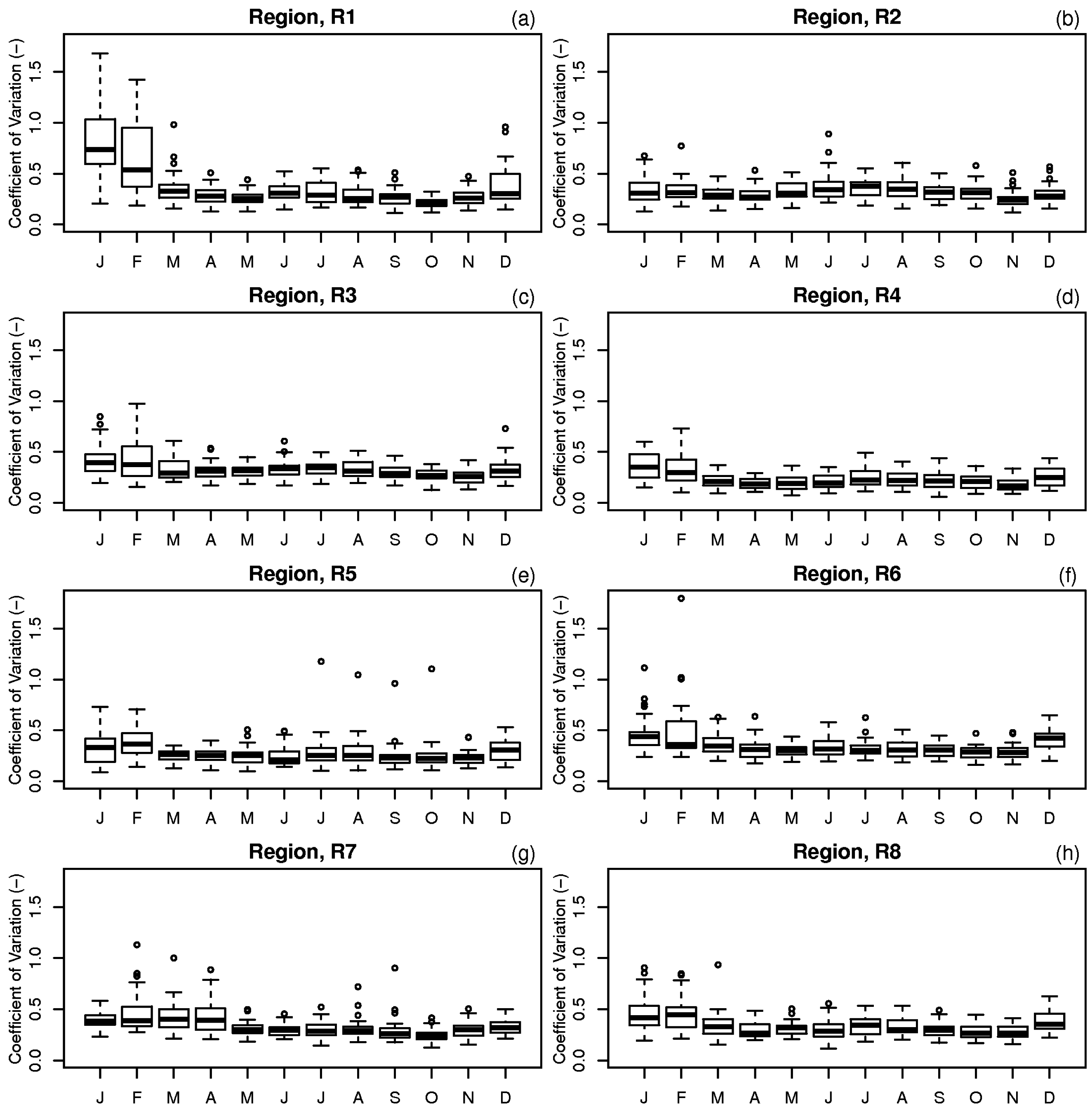
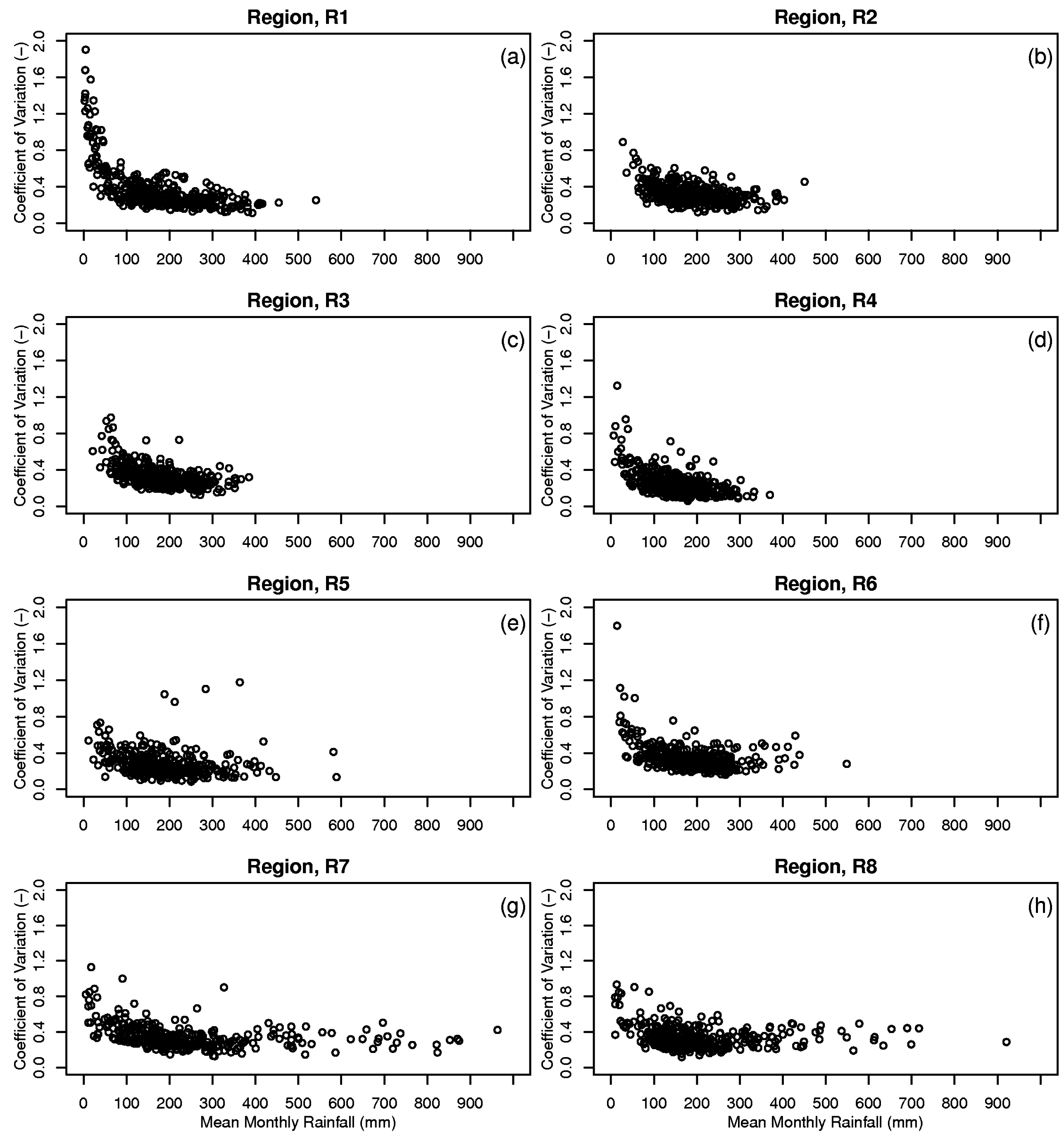
3.3. Spatial Variability

Figure 2 shows the mean monthly spatial variability for the eight climatic regions. It is noted that the spatial rainfall variation is more uniform throughout the year in the east coast regions (R7 and R8) as shown in Figure 2g,f, although both regions have the largest variation in mean monthly rainfall as indicated in Figure 1. The southwestern coast (R4 and R5) and west coast (R2 and R3) regions receive smaller amounts of monthly rainfall, but the spatial variation differs, particularly during monsoons. For the inland region (R6), the largest spatial variability occurs in February, the month with the smallest rainfall amount of 94 mm/month (refer to Figure 1). The larger range of coefficients of variation is most visible for all regions during the NEM, when the largest amount of rainfall is received over the east coast region (see Table 1), and to a smaller extent during the SWM.
The northern region (R1) shows the largest interquartile range (0.19) and mean monthly coefficients of variation (0.38) compared to the other regions. In contrast, the northern part of the southwest region (R4) has a smaller interquartile range (0.13) and lowest mean monthly coefficients of variation (0.25), indicating that the areal rainfall is more uniformly distributed. The calculated median values of the coefficients of variation are close to the mean values for all regions, which suggest that the spatial rainfall variation is symmetrically distributed.
Figure 3 shows the coefficients of variation as a function of the spatial mean monthly rainfall for each climatic region. The relative coefficients of variation generally decreases exponentially with increasing mean monthly rainfall before reaching about 150 mm/month. The coefficients of variation remain fairly constant at 0.30 for mean monthly rainfall exceeding 150 mm/month. This implies the rainfall is more uniformly distributed across the region when the average rainfall amount is high. It is usually associated with heavy monsoon rainfall over the east coast of Peninsular Malaysia [43].
The topography and monsoon winds are likely the main factors controlling the magnitude of the spatial rainfall variation in the country. The Titiwangsa Range is a mountain range that forms the backbone of the Peninsula. During the northeast monsoon (NEM), stronger winds blow to the exposed areas, e.g., the east coast of Peninsular Malaysia [28,43,48], thus these areas receive substantial high amount of rainfall. Higher wind speeds promote more evaporation, which destabilizes the boundary layer and triggers deep convection, and hence, increases rainfall [49]. The inland and west coast areas, which are sheltered by mountain ranges, are relatively free from its influence. On the other hand, the southwest monsoon (SWM) wind speed is generally lighter. It tends to be wetter at the west coast of Peninsular Malaysia compared to the inland and east coast areas. The presence of mountain ranges separating the eastern and western parts of the Peninsula could be the best reason explaining the differences between the rainfall distributions of each region. The relatively flat landscape of the southern region (R5) and east coast regions (R7 and R8) result in reduced spatial rainfall variability.

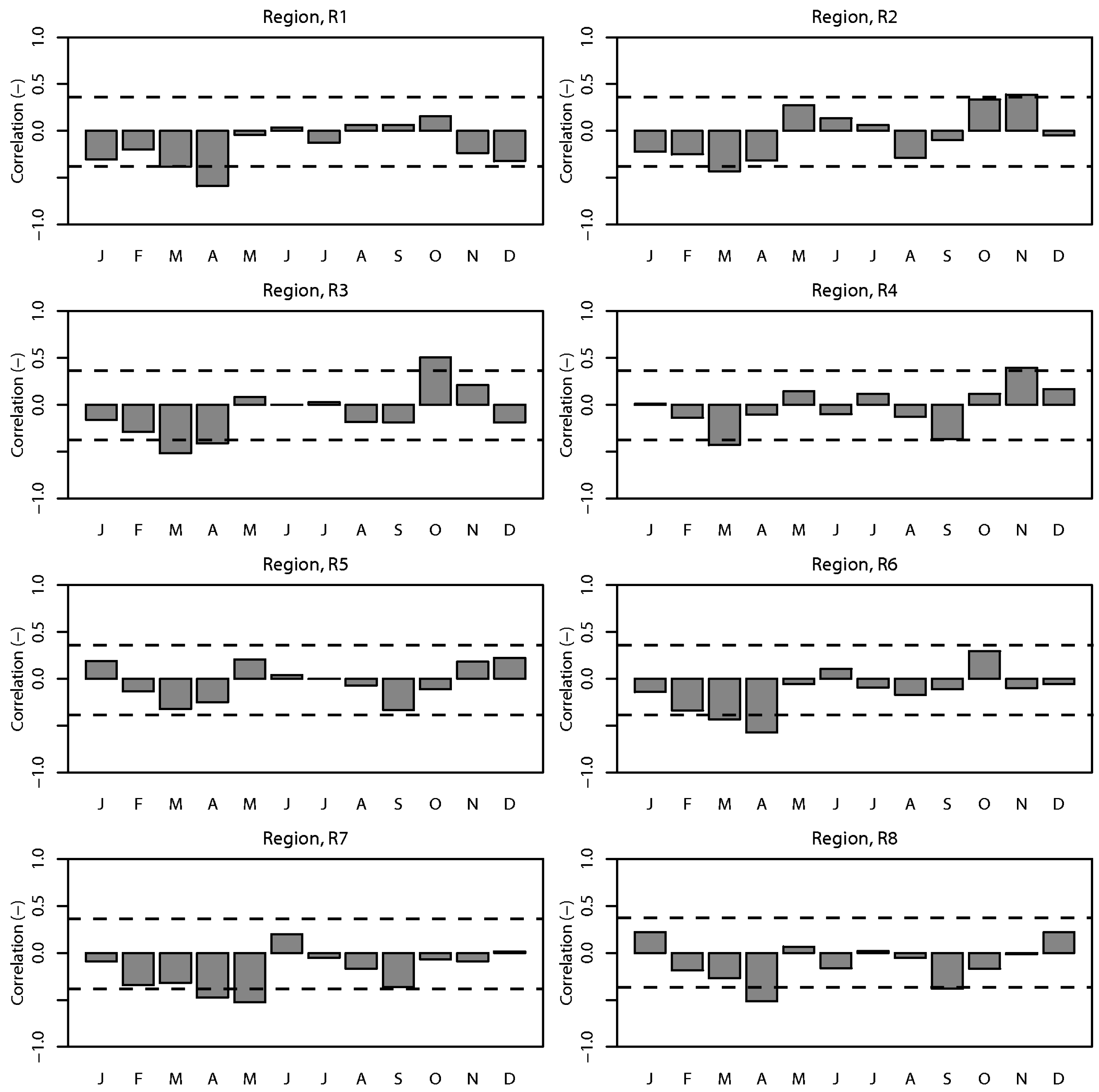
3.4. Influence of ENSO

The evolution of the ENSO [19,50] may have implications on the rainfall distribution over the Peninsula. The 31-year long-term rainfall anomaly for Peninsular Malaysia was, as a whole, found to be rather weakly and insignificantly (at 95% level) correlated (−0.19) with MEI. In addition, the monthly rainfall of all eight regions generally showed weak concurrent relationships with MEI. Figure 4 shows the correlation coefficients between the rainfalls over the Peninsula and MEI on monthly basis. The most obvious monthly rainfall-MEI correlation (−0.58) was seen in April during the inter-monsoon season. The relationships between monthly rainfalls and MEI of each region were also relatively weak (see Figure 5). These weak relationships are found to be consistent with findings of Juneng and Tangang [19]. The impact of ENSO on rainfall anomalies over the maritime continent has shown considerable spatial variation throughout the different phases of ENSO. During the SWM months, ENSO signature is largely confined to the south of the equator, induced by the interaction between the regional anomalous circulation and the background flow. This anomalous circulation is maintained by the regional feedback processes between the regional seas and the atmosphere. Hence the impact does not extend far northward to the Peninsular Malaysia. During the NEM months, the ENSO signature is shifted northeastward due to the establishment of the northwestern Pacific anticyclone/cyclone anomalies as the Rossby wave response to the surface heating/cooling. Due to the location of this anomalous circulation in the northwestern Pacific, the impact is largely confined to the northern Borneo and southern Philippines, but does not extend far westward to the Malay Peninsula. Thus, the concurrent impact of ENSO is generally weaker over the Peninsular Malaysia.
A lagged correlation analysis to determine potential lag/lead relationship between monsoon rainfall and MEI is presented in Table 5, showing the lagged correlation between monthly NEM rainfall and MEI for the eight climatic regions. The months of NEM rainfall are mostly correlated negatively with MEI during the NEM months, i.e., from November to March, suggesting modulation of drier conditions during the warm phase of ENSO events during ENSO mature months. The northwest zone (R1), west coast interior zone (R3) and central interior part (R6) of Peninsular Malaysia are correlated negatively with MEI at 95% level of significance. It is interesting to note that the NEM rainfalls posed positive correlation at 95% level of significance with MEI, with a delay of between five and eight months. The correlation magnitude is generally larger compared to the concurrent coefficient values. This means any ENSO (La Niña or El Niño) events could affect Peninsular Malaysia with a time lag of between five and eight months. The lagged correlation between monthly rainfalls of SWM and MEI was found to have similar correlation results as shown in Table 6 where monthly rainfalls are mostly correlated negatively with the MEI indicator during SWM monsoon months, with few regions (as highlighted in dark grey colour in Table 6) posting negative correlation at 95% level of significance in August and September. Generally, the monthly rainfalls of SWM monsoon correlated positively with MEI at 95% level of significance, with a delay of 4–8 months. The analysis clearly shows that the influence of ENSO on rainfall in Peninsular Malaysia is delayed by several months before posing implications to rainfall distributions, especially during SWM. The stronger lagged impact of ENSO on Peninsular rainfall may be explained by the capacitor effect [51] of ENSO which sees the tropical Indian Ocean acting as a heat capacitor during the decaying of a warm ENSO event. It is noted that after the dissipation of El Nino in the spring over the equatorial Pacific, the sea surface temperature over the tropical Indian Ocean remains anomalously warm. This causes the tropospheric temperature to increase by a moist adiabatic adjustment in deep convection, emanating a baroclinic Kelvin wave into the Pacific [51]. Numerical experiment by Xie et al. [51] suggests that this generates low pressure on the equator and anomalous anticyclone over the western north Pacific. The sea surface temperature over the South China Sea is anomalously warm and this promotes deep convective activities over the region. Hence, together with the lower pressure, the increases the rainfall anomalously over the region as shown by the positive lagged correlations in Table 6. Conventionally, the warm ENSO phases are associated with dry rainfall anomalies over Malaysia [17] during the development of ENSO events and this relationship was used to forecast the seasonal rainfall anomalies in the country [20]. The lagged positive relationship found in this study is an important consideration in predicting seasonal rainfall anomalies over Peninsular Malaysia with a longer lead time.

4. Conclusions

Statistically, Peninsular Malaysia can be differentiated into eight distinct rainfall regions. The results are generally in line with Lim [5] who classified subjectively the regional rainfall into five different zones based on pentad rainfall data. The differences between the current analysis and that of Lim [5] are (i) the east-west separation of the west coast zone; (ii) two different rainfall zones over south-west zone; and (ii) the east coast zone is divided into the northeastern zone covering parts of the states of Kelantan, Terengganu and Pahang, and southeastern zone covering large parts of Johor state.
The delineated rainfall zones are closely associated with the geography and topographic characteristics. The temporal variation of rainfall over the Peninsula is generally characterized by a bimodal distribution, i.e., a primary peak occurring during autumn transitional period and a secondary peak during the spring transitional period, except in the east coast zones with a single pronounced rainfall peak during the NEM. Generally, the NEM influence is relatively stronger and contributes more rainfall over all regions than the SWM. Significant increasing trends at the 95% confidence level have been found in the NEM rainfall for the northwest and west coast interior regions. The opposite is true during the SWM where most areas get drier due to decreases of rainfall over the year.
The east coast regions receive high monthly rainfall compared to other regions, but the rainfall is uniformly distributed spatially. For the southwestern coast and west coast regions, the spatial variation is more pronounced during monsoon periods, especially for NEM rainfalls. The larger range of the coefficients of variation is most visible during the NEM, and to a smaller extent during the SWM. The NEM also brings the largest amount of rainfall to the east coast region. It is noted that the inland regions, which received less rainfall in February, showed the largest spatial variation. The topography and monsoon winds are the main factors controlling the spatial rainfall variation in the country.
The relationship between monthly time series and MEI throughout the study period (31 years) showed a weakly negative correlation in the concurrent monthly rainfall and MEI for all regions. The influence of ENSO showed a correlation lag in the range of a 4–8 month period. Such delays may have implications for the rainfall distribution over the country, especially during NEM and SWM.
The results presented in this study demonstrate the advantages of using high quality gridded data sets in understanding hydrological regimes over Peninsular Malaysia. With a consistent spatio-temporal pattern of the data set, various precipitation indices can be properly defined, offering new insights to different hydrological regimes over the regions in the future. In addition, the enhanced understanding of the spatial and temporal rainfall variability is useful for more effective planning and management of water resources.

Acknowledgments

The authors thank the Department of Irrigation and Drainage Malaysia (DID), Malaysia Meteorological Department (MMD), and NOAA/NCDC for providing the data. Special thanks are also dedicated to Universiti Teknologi Malaysia for the financial support from Vote number RJ130000.7809.4F910.

Author Contributions

Chee Loong Wong and Juneng Liew designed the analytical framework and analyzed the data; Chee Loong Wong wrote the paper; Zulkifli Yusop, Tarmizi Ismail, Raymond Venneker and Stefan Uhlenbrook provided valuable comments on the papers.

Conflicts of Interest

The authors declare no conflict of interest. The founding sponsors had no role in the design of the study; in the collection, analyses, or interpretation of data; in the writing of the manuscript, nor in the decision to publish the results.

References

  1. Sato, Y.; Ma, X.; Xu, J.; Matsuoka, M.; Zheng, H. Analysis of long-term water balance in the source area of the Yellow river basin. Hydrol. Process. 2008, 22, 1618–1629. [Google Scholar] [CrossRef]
  2. Yang, D.; Li, C.; Hu, H.; Lei, Z.; Yang, S.; Kususa, T.; Koike, T.; Musiake, K. Analysis of water resources variability in the Yellow river of china during the last half century using historical data. Water Resour. Res. 2004, 40, W06502. [Google Scholar] [CrossRef]
  3. Abbaspour, K.C.; Rouholahnejad, E.; Vaghefi, S.; Srinivasan, R.; Yang, H.; Kløve, B. A continental-scale hydrology and water quality model for europe: Calibration and uncertainty of a high-resolution large-scale SWAT model. J. Hydrol. 2015, 524, 733–752. [Google Scholar] [CrossRef]
  4. Thornthwaite, C.W. An approach toward a rational classification of climate. Geogr. Rev. 1948, 38, 55–94. [Google Scholar] [CrossRef]
  5. Lim, J.T. Rainfall minimum in peninsular Malaysia during the northeast monsoon. Mon. Weather Rev. 1976, 104, 96–99. [Google Scholar] [CrossRef]
  6. Deni, S.M.; Jemain, A.A.; Ibrahim, K. Fitting optimum order of markov chain models for daily rainfall occurrences in peninsular Malaysia. Theor. Appl. Climatol. 2009, 97, 109–121. [Google Scholar] [CrossRef]
  7. Suhaila, J.; Jemain, A.A. Investigating the impacts of adjoining wet days on the distribution of daily rainfall amounts in peninsular Malaysia. J. Hydrol. 2009, 368, 17–25. [Google Scholar] [CrossRef]
  8. Suhaila, J.; Yusop, Z. Spatial and temporal variabilities of rainfall data using functional data analysis. Theor. Appl. Climatol. 2016. [Google Scholar] [CrossRef]
  9. Deni, S.M.; Suhaila, J.; Wan, Z.W.Z.; Jemain, A.A. Spatial trends of dry spells over peninsular Malaysia during monsoon seasons. Theor. Appl. Climatol. 2009, 99, 357–371. [Google Scholar] [CrossRef]
  10. Bishop, I.D. Provisional climatic regions in peninsular Malaysia. Pertanika 1984, 7, 19–24. [Google Scholar]
  11. Nieuwolt, S. Tropical rainfall variability—The agroclimatic impact. Agric. Environ. 1982, 7, 135–148. [Google Scholar] [CrossRef]
  12. Desa, M.N.; Niemczynowicz, J. Temporal and spatial characteristics in Kuala Lumpur, Malaysia. Atmos. Res. 1996, 42, 263–277. [Google Scholar] [CrossRef]
  13. Noguchi, S.; Nik, A.R. Rainfall characteristics of tropical rain forest and temperate forest: Comparison between bukit tarek in peninsular Malaysia and hitachi ohta in Japan. J. Trop. For. Sci. 1996, 9, 206–220. [Google Scholar]
  14. Economic Planning Unit. Masterplan for the Development of Water Resources in Peninsular Malaysia 2000–2050; Economic Planning Unit, Prime Minister’s Department: Kuala Lumpur, Malaysia, 1999.
  15. Department of Irrigation and Drainage. Review of the National Water Resources Study (2000–2050) and Formulation of National Water Resources Policy; Department of Irrigation and Drainage Malaysia: Kuala Lumpur, Malaysia, 2011.
  16. Tangang, F.T. Low frequency and quasi-biennial oscillations in the Malaysian precipitation anomaly. Int. J. Climatol. 2001, 21, 1199–1210. [Google Scholar] [CrossRef]
  17. Tangang, F.T.; Juneng, L. Mechanism of Malaysian rainfall anomalies. J. Clim. 2004, 17, 3616–3622. [Google Scholar] [CrossRef]
  18. Chan, N.W. Impacts of disasters and disaster risk management in Malaysia: The case of floods. In Resilience and Recovery in Asian Disasters: Community Ties, Market Mechanisms, and Governance; Aldrich, D.P., Oum, S., Sawada, Y., Eds.; Springer: Tokyo, Japan, 2015; pp. 239–265. [Google Scholar]
  19. Juneng, L.; Tangang, F.T. Evolution of enso-related rainfall anomalies in southeast Asia region and its relationship with atmosphere-ocean variations in indo-pacific sector. Clim. Dyn. 2005, 25, 337–350. [Google Scholar] [CrossRef]
  20. Juneng, L.; Tangang, F.T. Level and source of predictability of seasonal rainfall anomalies in Malaysia using canonical correlation analysis. Int. J. Climatol. 2008, 28, 1255–1267. [Google Scholar] [CrossRef]
  21. Tangang, F.T.; Juneng, L.; Ahmad, S. Trend and interannual variability of temperature in Malaysia: 1961–2002. Theor. Appl. Climatol. 2006, 89, 127–141. [Google Scholar] [CrossRef]
  22. Ng, M.W.; Camerlengo, A.; Khairi, A.A.W. A study of global warming in Malaysia. Jurnal Teknol. 2005, 42, 1–10. [Google Scholar]
  23. Moten, S. Multiple time scales in rainfall variability. J. Earth Syst. Sci. 1993, 102, 249–263. [Google Scholar]
  24. Groisman, P.Y.; Legates, D.R. Documenting and detecting long-term precipitation trends: Where are we and what should be done. Clim. Chang. 1995, 31, 601–622. [Google Scholar] [CrossRef]
  25. Yatagai, A.; Alpert, P.; Xie, P. Development of a daily gridded precipitation data set for the middle east. Adv. Geosci. 2008, 12, 1–6. [Google Scholar] [CrossRef]
  26. New, M.; Todd, M.; Hulme, M.; Jones, P. Precipitation measurements and trends in the twentieth century. Int. J. Climatol. 2001, 21, 1899–1922. [Google Scholar] [CrossRef]
  27. Wong, C.L.; Venneker, R.; Jamil, A.B.M.; Uhlenbrook, S. Development of a gridded daily hydrometeorological data set for peninsular Malaysia. Hydrol. Process. 2011, 25, 1009–1020. [Google Scholar] [CrossRef]
  28. Camerlengo, A.; Demmler, M.I. Wind-driven circulation of peninsular Malaysia’s eastern continental shelf. Sci. Mar. 1997, 61, 203–211. [Google Scholar]
  29. Shepard, D. A Two-dimensional Interpolation Function for Irregularly-spaced Data. In Proceedings of the 1968 23rd ACM National Conference, New York, NY, USA, 27–29 August 1968; ACM: New York, NY, USA, 1968; pp. 517–524. [Google Scholar]
  30. MacQueen, J.B. Some Methods for Classification and Analysis of Multivariate Observations. In Proceedings of the Fifth Berkeley Symposium on Mathematical Statistics and Probability, Oakland, CA, USA, 21 June–18 July 1965; University of California Press: Berkeley, CA, USA, 1967; Volume 1, pp. 281–297. [Google Scholar]
  31. Von Storch, H.; Zwiers, F.W. Statistical Analysis in Climate Research; Cambridge University Press: Cambridge, UK, 1999. [Google Scholar]
  32. Joliffe, I.T. Principal Component Analysis; Springer: New York, NY, USA, 1986; p. 271. [Google Scholar]
  33. Rousseeuw, P.J. Silhouettes: A graphical aid to the interpretation and validation of cluster analysis. J. Comput. Appl. Math. 1987, 20, 53–65. [Google Scholar] [CrossRef]
  34. Kendall, M.G. Rank Correlation Methods; Hafner: New York, NY, USA, 1948. [Google Scholar]
  35. Mann, H.B. Non-parametric test against trend. Econometrika 1945, 13, 245–259. [Google Scholar] [CrossRef]
  36. Zhang, X.; Harvey, K.D.; Hogg, W.D.; Yuzyk, T.R. Trends in canadian streamflow. Water Resour. Res. 2001, 37, 987–998. [Google Scholar] [CrossRef]
  37. Liu, Q.; Yang, Z.; Cui, B. Spatial and temporal variability of annual precipitation during 1961–2006 in yellow river basin, China. J. Hydrol. 2006, 361, 330–338. [Google Scholar] [CrossRef]
  38. Burn, D.H.; Elnur, M.A.H. Detection of hydrologic trends and variability. J. Hydrol. 2002, 255, 107–122. [Google Scholar] [CrossRef]
  39. Wolter, K.; Timlin, M.S. El niño/southern oscillation behaviour since 1871 as diagnosed in an extended multivariate enso index (mei.Ext). Int. J. Climatol. 2011, 31, 1074–1087. [Google Scholar] [CrossRef]
  40. Dale, W.L. The rainfall of Malaya, Part I. J. Trop. Geogr. 1959, 13, 23–37. [Google Scholar]
  41. Chang, C.P.; Harr, P.A.; Chen, H.J. Sypnotic disturbancess over the equatorial south china sea and western maritime continent during boreal winter. Mon. Weather Rev. 2005, 113, 489–503. [Google Scholar] [CrossRef]
  42. Salimum, E.; Tangang, F.T.; Juneng, L. Simulation of heavy precipitation episode over eastern peninsular Malaysia using mm5: Sensitivity to cumulus parameterization schemes. Meteorol. Atmos. Phys. 2010, 107, 33–49. [Google Scholar] [CrossRef]
  43. Juneng, L.; Tangang, F.T.; Reason, C.J.C. Numerical case study of an extreme rainfall event during 9–11 December 2004 over the east coast of peninsular Malaysia. Meteorol. Atmos. Phys. 2007, 98, 81–98. [Google Scholar] [CrossRef]
  44. Joseph, B.; Bhatt, B.C.; Koh, T.Y.; Chen, S. Sea breeze simulation over the malay peninsular in an intermonsoon period. J. Geophys. Res. 2008, 113, D20122. [Google Scholar] [CrossRef]
  45. Sow, K.S.; Juneng, L.; Tangang, F.T.; Hussin, A.G.; Mahmud, M. Numerical simulation of a severe late afternoon thunderstorm over peninsular Malaysia. Asmos. Res. 2011, 99, 248–262. [Google Scholar] [CrossRef]
  46. Varikoden, H.; Samah, A.A.; Babu, C.A. Spatial and temporal characteristics of rain intensity in the peninsular malaysia using trmm rain rate. J. Hydrol. 2010, 387, 312–319. [Google Scholar] [CrossRef]
  47. Nieuwolt, S. Diurnal rainfall variation in Malaya. Ann. Assoc. Am. Geogr. 1968, 58, 313–326. [Google Scholar] [CrossRef]
  48. Lim, E.S.; Das, U.; Pan, C.J.; Abdullah, K.; Wong, C.J. Investigating variability of outgoing longwave radiation over peninsular Malaysia using wavelet transform. J. Clim. 2013, 26, 3415–3428. [Google Scholar] [CrossRef]
  49. Back, L.E.; Bretherton, C.S. The relationship between wind speed and precipitation in the pacific itcz. J. Clim. 2005, 18, 4317–4328. [Google Scholar] [CrossRef]
  50. Cheang, B.K. Interannual variability of monsoons in malaysia and its relationship with ENSO. J. Earth Syst. Sci. 1993, 102, 219–239. [Google Scholar]
  51. Xie, S.-P.; Hu, K.; Hafner, J.; Tokinaga, H.; Du, Y.; Huang, G.; Sampe, T. Indian Ocean capacitor effect on Indo-western Pacific climate during the summer following El Niño. J. Clim. 2009, 22, 730–747. [Google Scholar] [CrossRef]
Figure 1. Box and whisker plot of areal average mean monthly rainfall (1976–2006) of the eight delineated rainfall regions in Malaysia. The solid line is the median, the height of the box is the difference between the third and first quartiles (IQR). The zones delineated by Lim [5] are shown in red lines.
Water 08 00500 g001
Figure 2. Box and whisker plot of mean monthly coefficients of spatial variations (1976–2006) of the eight delineated rainfall regions (Panel a to h). The solid line is the median, the height of the box is the difference between the third and first quartiles (IQR). Any data observation which lies 1.5 IQR lower than the first quartile or 1.5 IQR higher than the third quartile is considered an outlier in the statistical sense, indicated by open circles.
Water 08 00500 g002
Figure 3. Mean monthly rainfall coefficients of variation over the eight delineated rainfall regions (Panel a to h) for the period of 1976–2006.
Water 08 00500 g003
Figure 4. The correlation of concurrent monthly rainfall (mm/month) and Multivariate El Ninõ-Southern Oscillation (ENSO) Index (MEI) for Peninsular Malaysia. The dotted line indicates significance at 95% level.
Water 08 00500 g004
Figure 5. The correlation of concurrent monthly rainfall (mm/month) and Multivariate ENSO Index (MEI) of eight distinct climatic regions. The dotted line indicates significance at 95% level.
Water 08 00500 g005
Table 1. Averaged silhouette width, S ¯ indicates better grouping if closer to one.
K, Non-Overlapping Regions345678910
Averaged silhouette width, S ¯ 0.350.410.430.460.430.530.500.48
Table 2. Rainfall contributions in Peninsular Malaysia for the period of 1976–2006.
RegionMean Elevation (m) (min, max)Annual Rainfall (mm/Year)Standard DeviationNortheast Monsoon (Nov.–Mar.) RainfallSouthwest Monsoon (May–Sep.) RainfallTotal Monsoon Rainfall
mm/Year%mm/Year%mm/Year%
R1272
(0, 860)
211844056726103548160275
R2116
(0, 773)
22293149224180636172877
R3326
(16, 1475)
21543479214276535168678
R474
(0, 189)
18074647053974341144880
R550
(0, 183)
220660410044579435179881
R6457
(68, 1280)
21743298683986839173679
R7266
(0, 1044)
294032115305299333252385
R8128
(0, 352)
238355012685373530200484
Table 3. Annual and monsoons rainfall trends (mm/year) of eight distinct climatic regions for the period of 1976–2006.
RegionAnnualNEMSWM
R16.37.5−5.1
R23.74.3−1.5
R37.76.70.0
R42.13.1−1.8
R57.14.9−0.8
R65.85.0−1.0
R713.311.4−1.1
R89.15.8−0.3
Notes: Light grey indicates significant rainfall (mm) trend at 90% confidence level; Dark grey indicates significant rainfall (mm) trend at 95% confidence level; NEM: northeast monsoon; SWM: southwest monsoon.
Table 4. Monthly rainfall trends (mm/month) of eight distinct climatic regions.
RegionJan.Feb.Mar.Apr.MayJun.Jul.Aug.Sep.Oct.Nov.Dec.
R11.31.32.50.7−3.50.8−0.80.5−2.02.60.22.8
R21.60.3−0.20.1−1.70.3−0.30.5−0.20.31.71.5
R32.20.21.20.8−1.00.3−0.10.50.4−0.71.62.5
R42.0−1.31.1−0.2−0.3−0.2−0.61.1−2.00.1−0.93.1
R55.6−1.11.5−0.2−0.0−0.90.00.8−0.71.1−0.41.5
R62.20.21.70.3−1.40.9−0.90.9−0.60.1−0.52.8
R75.02.43.5−0.4−0.61.1−1.40.0−0.21.0−1.24.2
R85.80.11.1−0.1−0.5−0.1−0.20.9−0.40.8−0.32.0
Notes: Light grey indicates significant monthly rainfall (mm/month) trend at 90% confidence level; Dark grey indicates significant monthly rainfall (mm/month) trend at 95% confidence level.
Table 5. Correlation coefficient values between the NEM rainfall and the MEI at various concurrent and leading months.
RegionMar.Apr.MayJun.Jul.Aug.Sep.Oct.Nov.Dec.Jan.Feb.Mar.
R10.2320.2150.2690.053−0.118−0.222−0.267−0.342−0.435−0.478−0.489−0.537−0.536
R20.4890.5630.5850.4530.2300.045−0.051−0.057−0.153−0.223−0.243−0.284−0.287
R30.3080.3440.3480.2030.002−0.143−0.244−0.236−0.319−0.393−0.394−0.444−0.470
R40.2930.3920.4080.4140.2800.1460.0300.055−0.023−0.087−0.071−0.114−0.128
R50.3960.4390.3950.3630.2590.1660.1000.1470.0590.0450.0560.012−0.011
R60.5420.5270.5590.3000.048−0.106−0.212−0.265−0.383−0.394−0.401−0.486−0.478
R70.4260.4510.5230.3350.1530.046−0.036−0.112−0.247−0.2350.201−0.258−0.264
R80.5380.5820.5890.5290.3410.2220.1450.1360.0220.0400.052−0.007−0.016
Notes: Light grey indicates significant correlation coefficient at 90% confidence level; Dark grey indicates significant correlation coefficient at 95% confidence level.
Table 6. Correlation coefficient values between the SWM rainfall and the MEI at various concurrent and leading months.
RegionSep.Oct.Nov.Dec.Jan.Feb.Mar.Apr.MayJun.Jul.Aug.Sep.
R10.3950.4110.3810.3980.4050.3550.3300.2800.2550.2180.086−0.024−0.090
R20.4620.4230.4250.4510.4480.4190.4010.3800.3820.2130.040−0.117−0.219
R30.3730.3230.2850.3410.3320.2650.2500.2530.2490.061−0.128−0.249−0.308
R40.5270.4500.3710.3890.3710.3280.3220.2880.201−0.060−0.205−0.375−0.464
R50.5760.5630.5390.5900.6370.5890.5650.5580.4650.201−0.085−0.270−0.321
R60.2920.2790.2120.2520.2540.2230.2420.2090.2050.040−0.156−0.280−0.326
R70.3560.3460.2630.2580.2250.2170.2020.054−0.035−0.189−0.335−0.472−0.499
R80.5050.4460.3400.3810.3900.3290.2940.2390.130−0.094−0.254−0.378−0.423
Notes: Light grey indicates significant correlation coefficient at 90% confidence level; Dark grey indicates significant correlation coefficient at 95% confidence level.

