
Simulation and Prediction of Climate Variability and Assessment of the Response of Water Resources in a Typical Watershed in China

Abstract
:1. Introduction
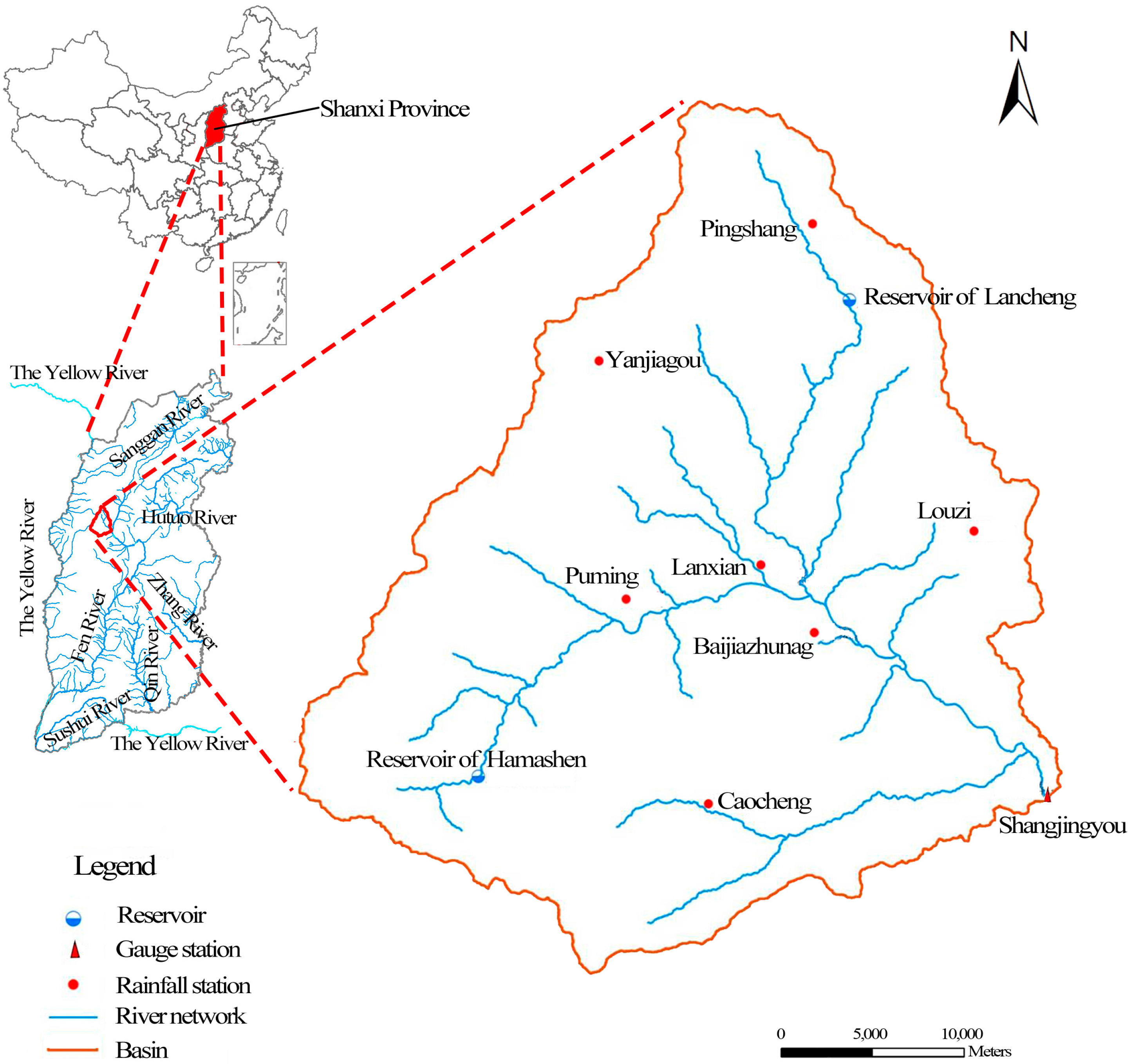
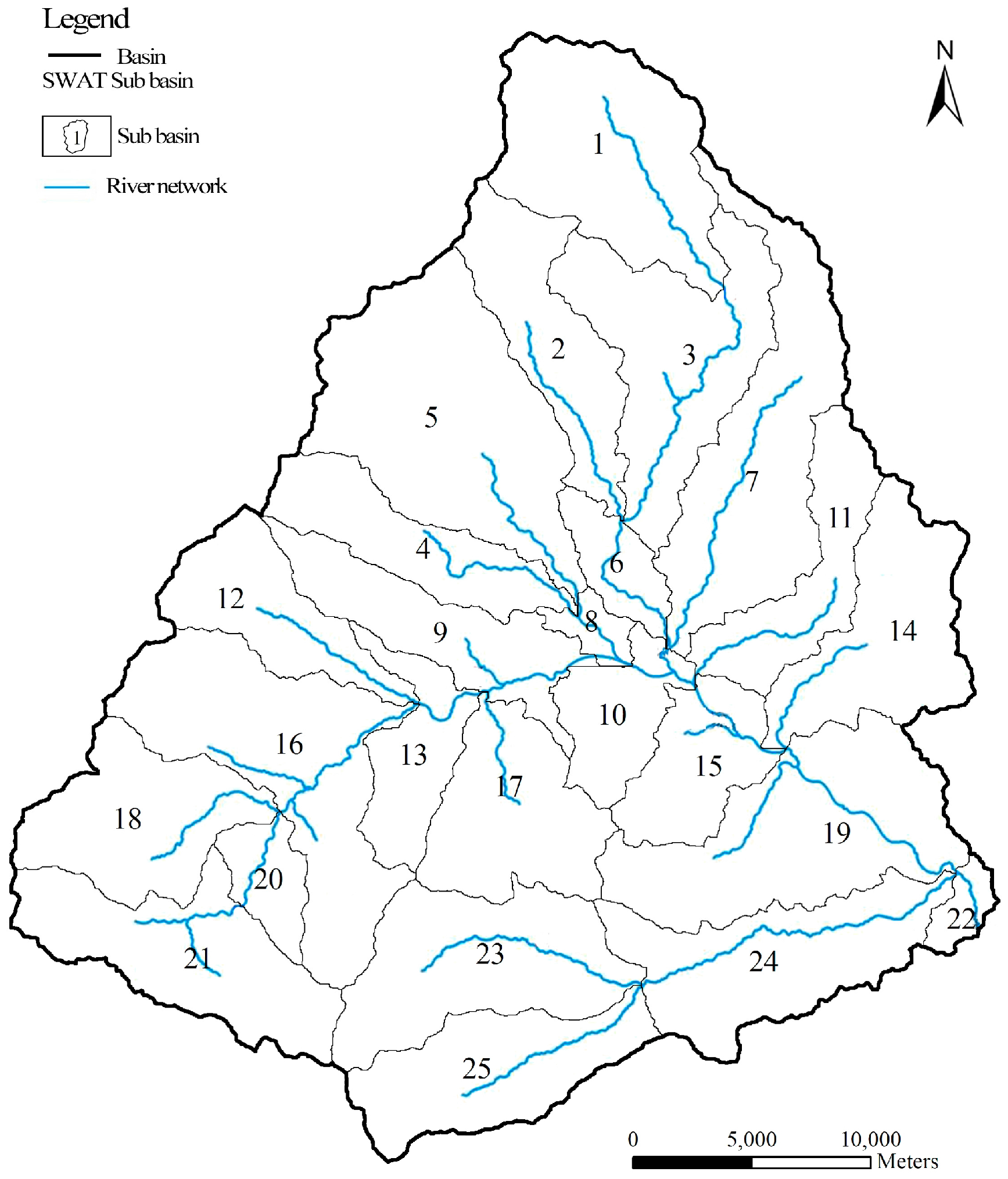
2. Study Area
3. Methodology and Materials
3.1. SWAT (Soil and Water Assessment Tool) Model
3.2. Model Setup
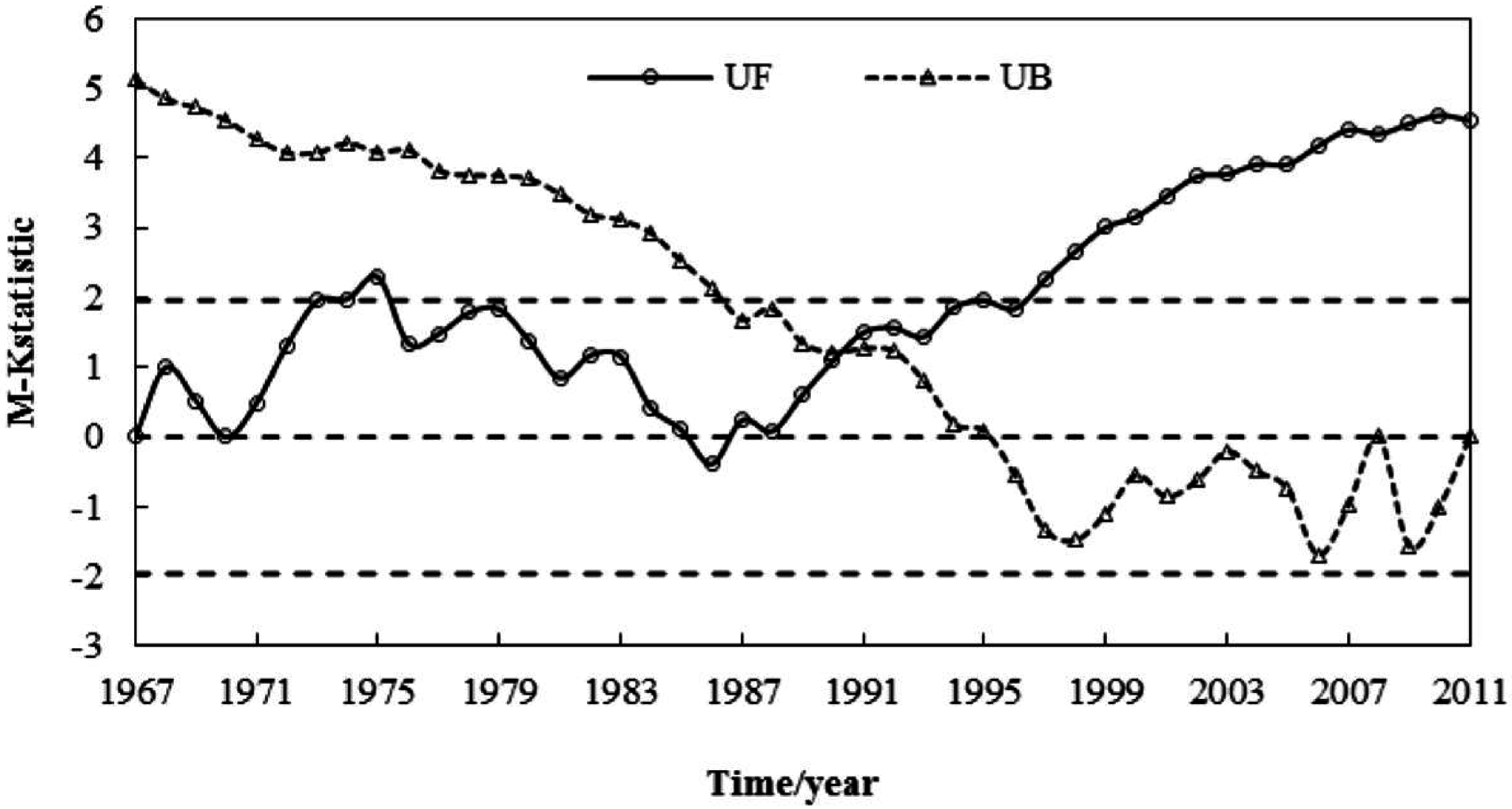
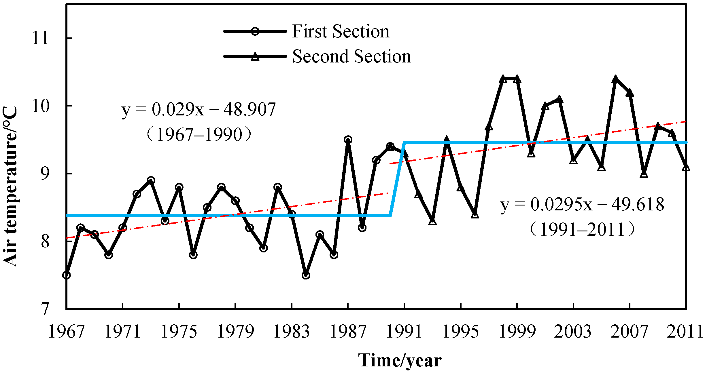
3.2.1. Data Collection and Analysis
3.2.2. Characterization and Delineation of Hydrological Response Units
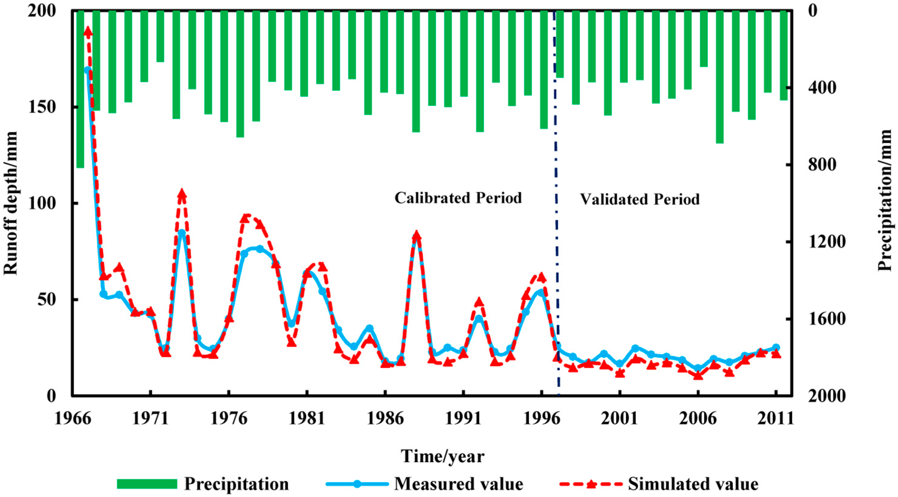
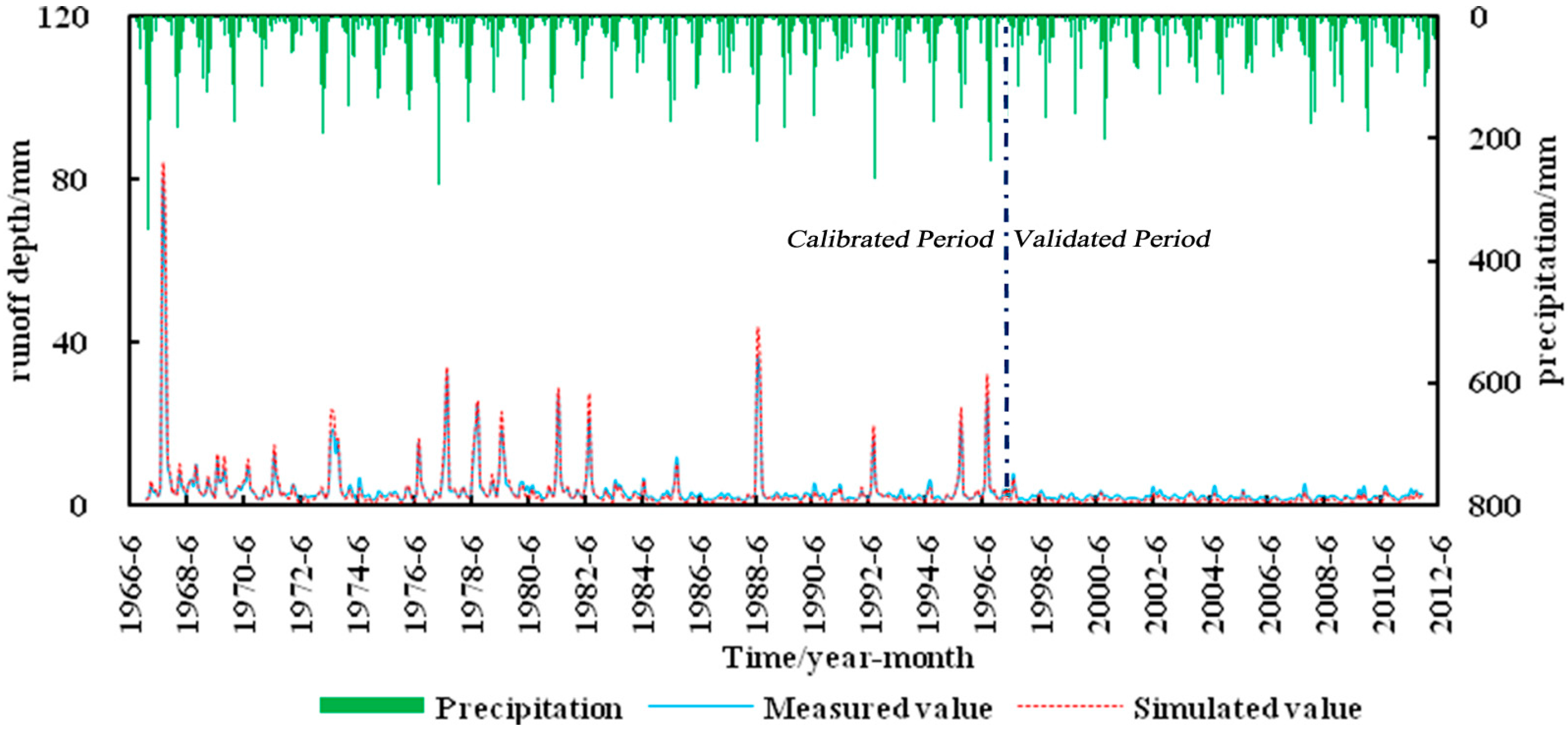
3.2.3. Model Calibration and Validation
3.3. Scenarios of Climate Change
3.3.1. Design of the Climate Scenarios
3.3.2. Methods of Sensitivity Analysis
4. Results and Discussion
4.1. SWAT Model Calibration and Validation Results
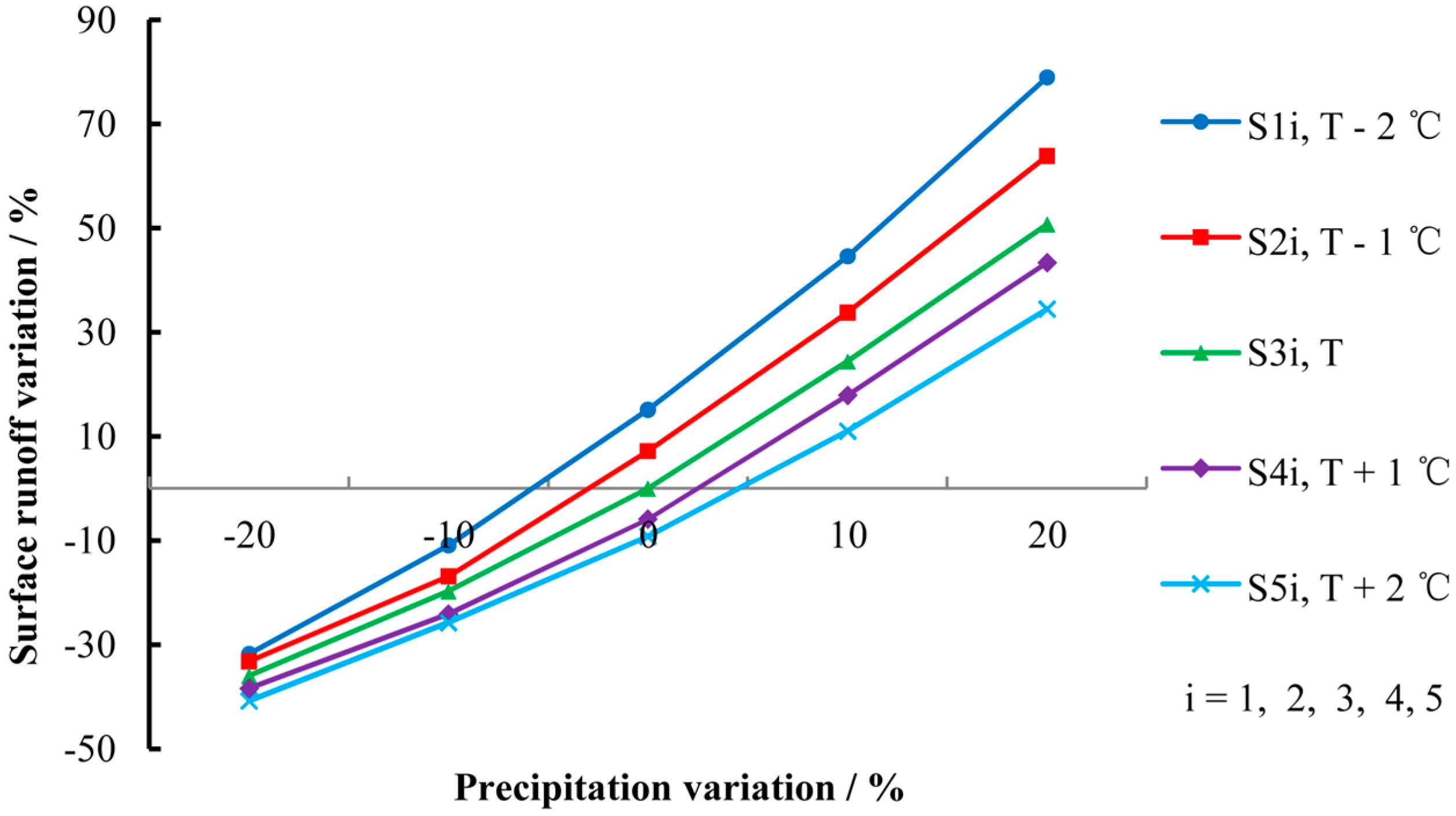
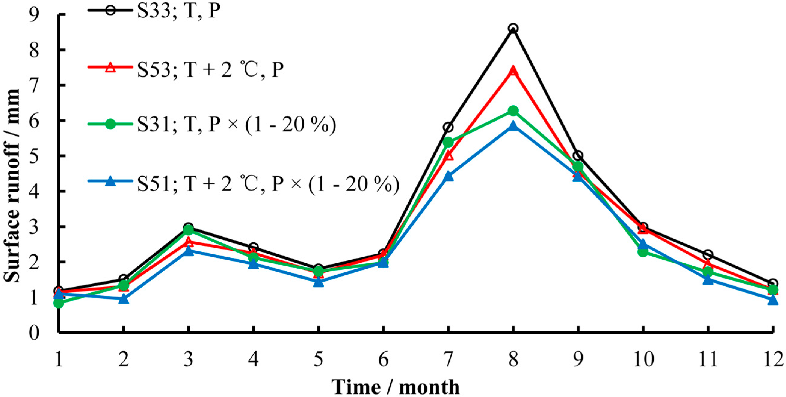
4.2. Sensitivity Analysis of Surface Runoff
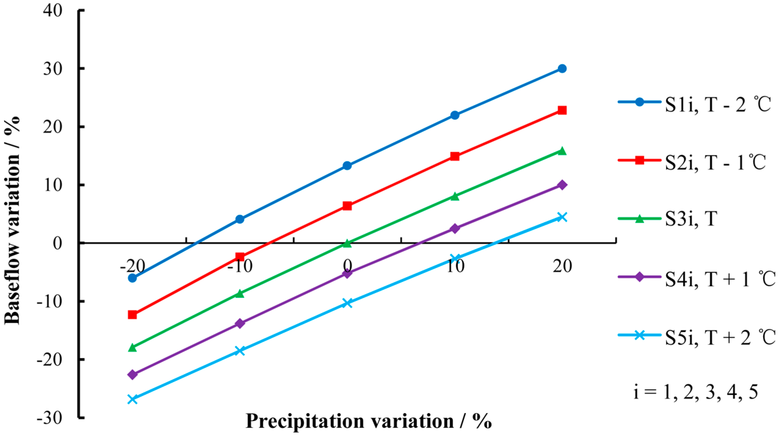
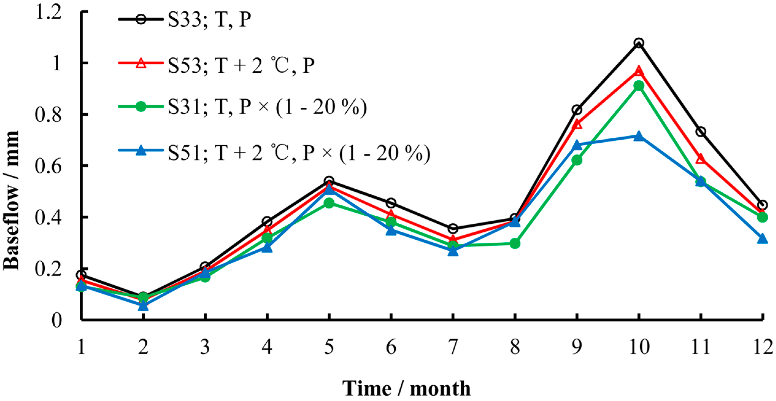
4.3 Sensitivity Analysis of Baseflow
5. Conclusions
Acknowledgments
Author Contributions
Conflicts of Interest
References
- Palazzoli, I.; Maskey, S.; Uhlenbrook, S.; Nana, E.; Bocchiola, D. Impact of prospective climate change on water resources and crop yields in the Indrawati basin, Nepal. Agric. Syst. 2015, 133, 143–157. [Google Scholar] [CrossRef]
- Xu, Y.P.; Zhang, X.J.; Ran, Q.H.; Tian, Y. Impact of climate change on hydrology of upper reaches of Qiantang River Basin, East China. J. Hydrol. 2013, 483, 51–60. [Google Scholar] [CrossRef]
- Luo, Y.Z.; Ficklin, D.L.; Liu, X.M.; Zhang, M.H. Assessment of climate change impacts on hydrology and water quality with a watershed modeling approach. Sci. Total Environ. 2013, 450–451, 72–82. [Google Scholar] [CrossRef] [PubMed]
- Iensen, I.R.R.; Schultz, G.B.; Santos, I.D. Simulation of hydrosedimentological impacts caused by climate change in the Apucaraninha River watershed, southern Brazil. In Proceedings of the Symposium Held in New Orleans, Louisiana, USA, 11–14 December 2014.
- Githui, F.; Gitau, W.; Mutua, F.; Bauwens, W. Climate change impact on SWAT simulated streamflow in western Kenya. Int. J. Climatol. 2009, 29, 1823–1834. [Google Scholar] [CrossRef]
- Füssel, H.-M. Review and Quantitative Analysis of Indices of Climate Change Exposure, Adaptive Capacity, Sensitivity, and Impacts. 2010. Available online: https://openknowledge.worldbank.org/handle/10986/9193 (accessed on 20 July 2015).
- Karamouz, M.; Goharian, E.; Nazif, S. Reliability Assessment of the water supply systems under uncertain future extreme climate conditions. Earth Interact. 2013, 17, 1–27. [Google Scholar] [CrossRef]
- Fowler, H.J.; Kilsby, C.G.; O’Connell, P.E. Modeling the impacts of climatic change and variability on the reliability, resilience, and vulnerability of a water resource system. Water Resour. Res. 2003, 39, 2503–2512. [Google Scholar] [CrossRef]
- Liu, Y.; Ren, L.L.; Hong, Y.; Zhu, Y.; Yang, X.L.; Yuan, F.; Jiang, S.H. Sensitivity analysis of standardization procedures in drought indices to varied input data selections. J. Hydrol. 2016, 538, 817–830. [Google Scholar] [CrossRef]
- Zhang, L.H.; Yan, J.P.; Liu, L.S. Climate change and drought and flood disasters trend in Shanxi. J. Arid Land Resour. Environ. 2013. (In Chinese) [Google Scholar] [CrossRef]
- Ning, T.; Guo, Z.S.; Guo, M.C.; Han, B. Soil water resources use limit in the loess plateau of China. Agric. Sci. 2013, 14, 100–105. [Google Scholar] [CrossRef]
- Lv, Z.M.; Li, Z.; Li, J.J.; Dai, R.R. Verifying the applicability of PRECIS-simulated precipitation on the Loess Plateau. Acta Ecol. Sin. 2016, 36. (In Chinese) [Google Scholar] [CrossRef]
- Kang, N.; Yang, Y.G.; Li, H.J.; Li, J.C. A study on water environmental carrying capacity of typical mining area in Loess Plateau. Bull. Soil Water Conserv. 2015, 35, 274–280. (In Chinese) [Google Scholar]
- Tan, H.B.; Jin, B.; Wang, R.A.; Zhang, Y.D.; Liu, Z.H. Climate change, human activity and water resources issues in loess hilly areas in Pingliang. Water Resour. Prot. 2015, 31, 45–51. (In Chinese) [Google Scholar]
- Zeng, S.D.; Xia, J.; She, D.X.; Du, H.; Zhang, L.P. Impacts of climate change on water resources in the Luan River basin in North China. Water Int. 2012, 5, 552–563. [Google Scholar] [CrossRef]
- Goharian, E.; Burian, S.; Bardsley, T.; Strong, C. Incorporating Potential Severity into Vulnerability Assessment of Water Supply Systems under Climate Change Conditions. J. Water Resour. Plann. Manag. 2015. [Google Scholar] [CrossRef]
- Asefa, T.; Clayton, J.; Adams, A.; Anderson, D. Performance evaluation of a water resources system under varying climatic conditions: Reliability, resilience, vulnerability and beyond. J. Hydrol. 2014, 508, 53–65. [Google Scholar] [CrossRef]
- Miller, W.P.; Piechota, T.C.; Gangopadhyay, S.; Pruitt, T. Development of streamflow projections under changing climate conditions over Colorado River basin headwaters. Hydrol. Earth Syst. Sci. 2011, 15, 2145–2164. [Google Scholar] [CrossRef]
- Liu, M. Simulation and Prediction of Climate Change in Eastern China and Assessment of the Response of Hydrology and Water Quality in a Typical Watershed. Ph.D. Thesis, Zhejiang University, Hangzhou, China, April 2015. [Google Scholar]
- York, C.; Goharian, E.; Burian, S. Impacts of large-scale stormwater green infrastructure implementation and climate variability on receiving water response in the Salt Lake City area. Am. J. Environ. Sci. 2015, 11, 278–292. [Google Scholar] [CrossRef]
- Maurer, E.P.; Brekke, L.; Pruitt, T.; Duffy, P.B. Fine-resolution climate projections enhance regional climate change impact studies. Eos Trans. Am. Geophys. Union 2007, 88, 504. [Google Scholar] [CrossRef]
- Dudula, J.; Randhir, T.O. Modeling the influence of climate change on watershed systems: Adaptation through targeted practices. J. Hydrol. 2016. [Google Scholar] [CrossRef]
- Sood, A.; Muthuwatta, L.; McCartney, M.A. SWAT evaluation of the effect of climate change on the hydrology of the Volta River basin. Water Int. 2013, 38, 297–311. [Google Scholar] [CrossRef]
- Kirby, J.M.; Mainuddin, M.; Mpelasoka, F.; Ahmad, D.; Palash, W.; Quadir, M.E.; Shah-Newaz, S.M.; Hossain, M.M. The impact of climate change on regional water balances in Bangladesh. Clim. Chang. 2016, 135, 481–491. [Google Scholar] [CrossRef]
- Zahabiyoun, B.; Goodarzi, M.R.; Massah Bavani, A.R.; Azamathulla, H.M. Assessment of climate change impact on the Gharesou River Basin using SWAT hydrological model. Clean–Soil Air Water 2013, 41, 601–609. [Google Scholar] [CrossRef]
- Krysanova, V.; White, M. Advances in water resources assessment with SWAT—An overview. Hydrol. Sci. J. 2015, 60, 771–783. [Google Scholar] [CrossRef]
- Krysanova, V.; Arnold, J.G. Advances in ecohydrological modelling with SWAT—A review. Hydrol. Sci. J. 2008, 53, 939–947. [Google Scholar] [CrossRef]
- Gassman, P.W.; Sadeghi, A.M.; Srinivasan, R. Applications of the SWAT modle special section: Overview and insights. J. Environ. Qual. 2014, 43, 1–8. [Google Scholar] [CrossRef] [PubMed]
- Li, Z.; Liu, W.Z.; Zhang, X.C.; Zheng, F.L. Impacts of land use change and climate variability on hydrology in an agricultural catchment on the Loess Plateau of China. J. Hydrol. 2009, 377, 35–42. [Google Scholar] [CrossRef]
- Han, F.; Ren, L.; Zhang, X.; Li, Z. The WEPP Model application in a small watershed in the Loess Plateau. PLoS ONE 2016, 11, e0148445. [Google Scholar] [CrossRef] [PubMed]
- Zhu, Q. Research on Water Resources Responses to Climate Changes in Lanhe Watershed based on SWAT Model. Master’s Thesis, Taiyuan University of Technology, Taiyuan, China, June 2013. [Google Scholar]
- Gao, Z.Q. GM(1,2) time-lag model of mid-long term runoff forecasting on Lanhe River. J. Taiyuan Univ. Technol. 2006, 37, 71–73. (In Chinese) [Google Scholar]
- Liu, Y. Analysis on the hydrological characteristics of Lanhe watershed. Sci-Tech Inf. Dev. Econ. 2008, 18, 135–136. (In Chinese) [Google Scholar]
- Neitsch, S.L.; Arnold, J.G.; Kiniry, J.R.; Srinivasan, R.; Williams, J.R. Soil and Water Assessment Tool User’s Manual. Available online: http://swat.tamu.edu/media/1294/swatuserman.pdf (accessed on 3 June 2014).
- Neitsch, S.L.; Arnold, J.G.; Kiniry, J.T.; Williams, J.R. Soil and Water Assessment Tool. Theoretical Documentation Version 2009. Available online: http://swat.tamu.edu/media/99192/swat2009-theory.pdf (accessed on 3 June 2014).
- Moriasi, D.N.; Wilson, B.N.; Douglas-Mankin, K.R.; Arnold, J.G.; Gowda, P.H. Hydrologic and water quality models: Use, Calibration, and Validation. Trans. ASABE 2012, 55, 1241–1247. [Google Scholar] [CrossRef]
- Arnold, J.G.; Kiniry, J.R.; Srinivasan, R.; Williams, J.R.; Haney, E.B.; Neitsch, S.L. Soil and Water Assessment Tool Input/Output Documentation. Available online: http://swat.tamu.edu/media/69296/SWAT-IO-Documentation-2012.pdf (accessed on 3 June 2014).
- Moriasi, D.N.; Gitau, M.W.; Pai, N.; Daggupati, P. Hydrologic and water quality models: Performance measures and evaluation criteria. Trans. ASABE 2015, 58, 1763–1785. [Google Scholar]
- Malagó, A.; Venohr, M.; Gericke, A.; Vigiak, O.; Bouraoui, F.; Grizzetti, B.; Kovacs, A. Modelling nutrient pollution in the Danube River Basin: A comparative study of SWAT, MONERIS and GREEN models. Publ. Off. Eur. Union 2015. [Google Scholar] [CrossRef]
- Gassman, P.W.; Sadeghi, A.M.; Srinivasan, R. Applications of the SWAT model special section: Overview and insights. J. Environ. Qual. 2014, 43, 1–8. [Google Scholar] [CrossRef] [PubMed]
- Qiao, L.; Zou, C.B.; Will, R.E.; Stebler, E. Calibration of SWAT model for woody plant encroachment using paired experimental watershed data. J. Hydrol. 2015, 523, 231–239. [Google Scholar] [CrossRef]
- Bouslihim, Y.; Kacimi, I.; Brirhet, H.; Khatati, M.; Rochdi, A.; Pazza, N.E.A.; Miftah, A.; Yaslo, Z. Hydrologic modeling using SWAT and GIS, application to subwatershed Bab-Merzouka (Sebou, Morocco). J. Geogr. Inf. Syst. 2016, 8, 20–27. [Google Scholar] [CrossRef]
- Arnold, J.G.; Allen, P.M.; Bernhardt, G. A comprehensive surface groundwater flow model. J. Hydrol. 1993, 142, 47–69. [Google Scholar] [CrossRef]
- Vrochidou, A.-E.K.; Tsanis, I.K.; Grillakis, M.G.; Koutroulis, A.G. The impact of climate change on hydrometeorological droughts at a basin scale. J. Hydrol. 2013, 476, 290–301. [Google Scholar] [CrossRef]
- Koutroulis, A.G.; Tsanis, I.K.; Daliakopoulos, I.N.; Jacob, D. Impact of climate change on water resources status: A case study for Crete Island, Greece. J. Hydrol. 2013, 479, 146–158. [Google Scholar] [CrossRef]
- Liuzzo, L.; Noto, L.V.; Arnone, E.; Caracciolo, D.; Loggia, G.L. Modification in water resources availability under climate changes: A case study in a Sicilian basin. Water Resour. Manag. 2015, 29, 1117–1135. [Google Scholar] [CrossRef]
- Neupane, R.P.; White, J.D.; Alexander, S.E. Projected hydrologic changes in monsoon-dominated Himalaya Mountain basins with changing climate and deforestation. J. Hydrol. 2015, 525, 216–230. [Google Scholar] [CrossRef]
- Kannan, N.; White, S.M.; Worrall, F.; Whelan, M.J. Sensitivity analysis and identification of the best evapotranspiration and runoff options for hydrological modeling in SWAT-2000. J. Hydrol. 2007, 332, 456–466. [Google Scholar] [CrossRef]
- Arnold, J.G.; Moriasi, D.N.; Gassman, P.W.; Abbaspour, K.C.; White, M.J.; Srinivasan, R.; Santhi, C.; Harmel, R.D.; van Griensven, A.; van Liew, M.W.; et al. SWAT: Model use, calibration, and validation. Trans. ASABE 2012, 55, 1494–1508. [Google Scholar] [CrossRef]
- Jung, Y.W.; Oh, D.; Kim, M.; Park, J.W. Calibration of LEACHN model using LH-OAT sensitivity analysis. Nutr. Cycl. Agroecosyst. 2010, 87, 261–275. [Google Scholar] [CrossRef]
- Song, W.X.; Jiang, S.H.; Yang, C.S.; Wang, L.M. Impact of SCE-UA and SCEM-UA on improved HYMOD model. Water Resour. Power 2013, 31, 17–20. (In Chinese) [Google Scholar]
- Setegn, S.G.; Melesse, A.M.; Haiduk, A.; Webber, D.; Wang, X.; McClain, M.E. Modeling hydrological variability of fresh water resources in the Rio Cobre watershed, Jamaica. Catena 2014, 120, 81–90. [Google Scholar] [CrossRef]
- Van Liew, M.W.; Veith, T.L.; Bosch, D.D.; Arnold, J.G. Suitability of SWAT for the conservation effects assessment project: A comparison on USDA-ARS experimental watersheds. J. Hydrol. Eng. 2007, 12, 173–189. [Google Scholar] [CrossRef]
- Gan, R.; Luo, Y.; Zuo, Q.T.; Sun, L. Effects of projected climate change on the glacier and runoff generation in the Naryn River Basin, Central Asia. J. Hydrol. 2015, 523, 240–251. [Google Scholar] [CrossRef]
- Malagò, A.; Pagliero, L.; Bouraoui, F.; Franchini, M. Comparing calibrated parameter sets of the SWAT model for the Scandinavian and Iberian peninsulas. Hydrol. Sci. J. 2015, 60, 949–967. [Google Scholar] [CrossRef]
- Moriasi, D.N.; Arnold, J.G.; Van liew, M.W.; Bingner, R.L.; Harmel, R.D.; Veith, T.L. Model evaluation guidelines for systematic quantification of accuracy in watershed simulations. Trans. ASABE 2007, 50, 885–900. [Google Scholar] [CrossRef]
- Jankowfsky, S.; Branger, F.; Braud, I.; Rodriguez, F.; Debionne, S.; Viallet, P. Assessing anthropogenic influence on the hydrology of small peri-urban catchments: Development of the object-oriented PUMMA model by integrating urban and rural hydrological models. J. Hydrol. 2014, 517, 1056–1071. [Google Scholar] [CrossRef]
- Loliyana, V.D.; Patel, P.L. Trend analysis of climatic variables and their impact on stream flow using NAM model. In Proceedings of the 36th IAHR World Congress, Hague, The Netherlands, 28 June–3 July 2015.
- Liu, Z.P.; Wang, Y.Q.; Shao, M.G.; Jia, X.X.; Li, X.L. Spatiotemporal analysis of multiscalar drought characteristics across the Loess Plateau of China. J. Hydrol. 2016, 534, 281–299. [Google Scholar] [CrossRef]
- Du, S.Q.; Gu, H.H.; Wen, J.H.; Chen, K.; Rompaey, A.V. Detecting Flood Variations in Shanghai over 1949–2009 with Mann-Kendall Tests and a Newspaper-Based Database. Water 2015, 7, 1808–1824. [Google Scholar] [CrossRef]
- Chatterjee, S.; Bisai, D.; Khan, A. Detection of approximate potential trend turning points in temperature time series (1941–2010) for Asansol Weather Observation Station, West Bengal, India. Atmos. Clim. Sci. 2014, 4, 64–69. [Google Scholar] [CrossRef]


| Temperature | Precipitation (P) | ||||
|---|---|---|---|---|---|
| P × (1 − 20%) | P × (1 − 10%) | P | P × (1 + 10%) | P × (1 + 20%) | |
| T − 2 °C | S11 | S12 | S13 | S14 | S15 |
| T − 1 °C | S21 | S22 | S23 | S24 | S25 |
| T | S31 | S32 | S33 | S34 | S35 |
| T + 1 °C | S41 | S42 | S43 | S44 | S45 |
| T + 2 °C | S51 | S52 | S53 | S54 | S55 |
| Test Statistic | Calibration Period (1967–1996) | Validation Period (1997–2011) | ||
|---|---|---|---|---|
| Annual Runoff | Monthly Runoff | Annual Runoff | Monthly Runoff | |
| R2 | 0.95 | 0.84 | 0.9 | 0.78 |
| Ens | 0.78 | 0.72 | 0.74 | 0.67 |
| PBIAS | 0.6% | −9.1% | 22.1% | 18.8% |
| Parameters | File Suffixes | Lower and Upper Bound | Calibrated Value | Parameter Definition |
|---|---|---|---|---|
| CN2 | *.mgt | −25%~25% | 18% | SCS runoff curve number |
| SOL_AWC | *.sol | −25%~25% | 20% | Available water capacity of soil layer |
| SLOPE | *.hru | −25%~25% | 24% | Average slope of subbasin |
| SOL_K | *.sol | −25%~25% | 18% | Saturated hydraulic conductivity |
| ESCO | *.hru | 0.00~1.00 | 0.0067 | Soil evaporation compensation factor |
| SOL_Z | *.sol | −25%~25% | 24% | Depth from soil surface to bottom of layer |
| CANMX | *.hru | 0.00~10.00 mm | 0.023 mm | Maximum canopy storage |
| ALPHA_BF | *.gw | 0.00~1.00 | 0.97 | Base flow Alpha factor |
| Surface Runoff | Temperature | Precipitation | ||||
|---|---|---|---|---|---|---|
| −20% | −10% | 0 | 10% | 20% | ||
| Volume (103 m3) | T − 2 °C | 29,616.6 | 38,671.6 | 49,965.5 | 62,769.5 | 77,679.7 |
| T − 1 °C | 28,971.5 | 36,066.1 | 46,520.6 | 58,070.9 | 71,113.9 | |
| T | 27,787.2 | 34,830.7 | 43,411.0 | 53,998.2 | 65,430.8 | |
| T + 1 °C | 26,731.8 | 32,937.0 | 40,846.3 | 51,174.6 | 62,246.1 | |
| T + 2 °C | 25,682.0 | 32,228.5 | 39,396.4 | 48,188.3 | 58,345.4 | |
| Baseflow | Temperature | Precipitation | ||||
|---|---|---|---|---|---|---|
| −20% | −10% | 0 | 10% | 20% | ||
| Volume (103 m3) | T − 2 °C | 6076.0 | 6728.8 | 7323.5 | 7885.8 | 8402.9 |
| T − 1 °C | 5668.8 | 6308.7 | 6877.5 | 7426.9 | 7937.5 | |
| T | 5306.8 | 5907.9 | 6463.8 | 6987.4 | 7491.5 | |
| T + 1 °C | 5003.0 | 5571.8 | 6127.7 | 6625.4 | 7110.2 | |
| T + 2 °C | 4731.5 | 5268.0 | 5798.0 | 6289.3 | 6754.7 | |
© 2016 by the authors; licensee MDPI, Basel, Switzerland. This article is an open access article distributed under the terms and conditions of the Creative Commons Attribution (CC-BY) license (http://creativecommons.org/licenses/by/4.0/).
Share and Cite
Jin, H.; Zhu, Q.; Zhao, X.; Zhang, Y. Simulation and Prediction of Climate Variability and Assessment of the Response of Water Resources in a Typical Watershed in China. Water 2016, 8, 490. https://doi.org/10.3390/w8110490
Jin H, Zhu Q, Zhao X, Zhang Y. Simulation and Prediction of Climate Variability and Assessment of the Response of Water Resources in a Typical Watershed in China. Water. 2016; 8(11):490. https://doi.org/10.3390/w8110490
Chicago/Turabian StyleJin, Hua, Qiao Zhu, Xuehua Zhao, and Yongbo Zhang. 2016. "Simulation and Prediction of Climate Variability and Assessment of the Response of Water Resources in a Typical Watershed in China" Water 8, no. 11: 490. https://doi.org/10.3390/w8110490