Innovative Analysis of Runoff Temporal Behavior through Bayesian Networks

Abstract

Hydrological series are largely characterized by a strong random component in their behavior. More noticeable changes in the behavior patterns of rainfall/runoff temporal series are recently being observed. These modifications are not a trivial issue, especially in regards to peculiarities, non-linearities, diffused influences or higher time orders of dependence. This study mainly aimed to analyze the temporal dependence of an annual runoff series dynamically. This approach comprises a coupling between classic techniques (Autoregressive Moving Average Model, ARMA) and novel ones, based on Artificial Intelligent for hydrological research (Bayesian Networks, BNs). An ARMA model was built to provide reliable data to populate BNs. Then, causal reasoning, through Bayes’s theorem, allows the identification of the logic structure of temporal dependences within time series. Furthermore, the resultant conditional probability permits the quantification of the relative percentage of annual runoff change, and provides the right time order of dependence. This research introduces an original methodology able to build a logic structure for a stochastic analysis of temporal behavior. This approach also aimed to provide a powerful and graphic modeling method for improving the understanding of the dynamic runoff series temporal behavior. This was successfully demonstrated in two unregulated river basin stretches, belonging to the Duero river basin which is the largest basin in Spain.

1. Introduction

Meteorological events, mainly precipitation patterns and temperature records, and their subsequent hydrological effects are increasingly variable in a particular territory. Traditional temporal and spatial behavior patterns are being ever more modified over the world. In this sense, extreme events such as floods or droughts, among others, are more frequent in recent times [1,2,3,4]. There is a consequent strong necessity for powerful and reliable tools to build accurate models that reproduce the past and present hydrological behavior and forecast the future hydrological behavior of a river system. However, in order to build tools for dynamically analyzing the present behavior, as well as predicting the future, the historical behavior should be more deeply understood. In this sense, it has been recently shown that stationarity in hydrological time series is not as strict as in historical records. This fact, due to the increase of extreme events occurrence, means that the tools needed for prediction need to be much more flexible and powerful. For instance, a possible implication may be the need of designing tools able to deal with non-normal probability distributions.

Temporal behavior of hydrological analysis has been studied for some considerable time. Nowadays, many of those concepts and methodologies are valid benchmarks in stochastic hydrology [5,6]. Those concepts involve temporal–spatial correlation, statistical properties, including droughts and storage statistics, as well as trends, shifts and seasonality testing. Furthermore, time series analysis has been used for several applications such as filling in missing data, extending records, building mathematical models to generate synthetic hydrologic records, and detecting trends and shifts in hydrologic records, among others [7,8,9].

Nevertheless, a more complete and accurate time series analysis is needed, mainly because of the need to enhance the stochastic analysis. In this sense, traditional techniques describe the average temporal behavior of the time series largely deterministically or with some slight stochastic component. Additionally, it is necessary to have tools and/or methods that are able to analyze the influence of time steps on following ones within the time series, in a dynamic way. Furthermore, it is important to more accurately quantify the temporal dependency of time series to characterize water management scenarios and behavior patterns more realistically. This will allow a better assessment of water availability, and therefore, an optimum dimensioning of hydraulic infrastructures such as reservoirs.

This study aimed to dynamically analyze the temporal dependence of a runoff data series within a hydrological time series and to provide an estimation of the right time order (model order) of a hydrological time series. This is done through a hybrid method that comprises a combination of traditional techniques, (ARMA models), and new approaches based on Artificial Intelligent (Bayesian Networks).

Since this study comprises two river basins under different conditions (meteorological, morphodynamics, hydrological, hydraulic, etc.) this analysis will be useful for extrapolating to other similar basins. This research demonstrates that the proposed methodology can be an appropriate complement to traditional approaches.

Hydrological series are largely characterized by a strong random component in their intrinsic behavior [10]. A more sustainable and efficient management of basin water resources necessarily involves a deeper knowledge of time series’ behavior [7,9]. This comprises, among other factors, an analysis of the temporal evolution as well as the temporal dependence of hydrological variables such as precipitation, stream flows or total runoff [11,12].

It is well known that every model is an abstraction of the reality [13]. In this context, different approaches for hydrological modelling have been proposed since the middle of last century [14]. Therefore, in order to define an appropriate hydrological stochastic model, the main problem will be obtaining representative patterns of basin behavior. This definition should be largely based on features such as a goodness of fit, building lower complexity model (parsimonious model) and the maintenance of the statistical properties observed in the time series, among others [13,15]. Results from this model can be expressed in terms of probability for the involved stochastic processes.

Traditionally, stochastic hydrology models have been classified in two large groups: Parametric (PM) and nonparametric (NP). Among parametric models, the Autoregressive models (AR) [4,16,17,18], and Autoregressive Moving Average models (ARMA) have had great acceptance, as seen in [19,20,21,22,23]. Generally, these models have been applied to stationary time series [24,25], usually used for modeling low-order annual hydrologic time series, and they are characterized by their simplicity and versatility [22]. Furthermore, the hybridization with NP ensures that non-stationary and higher order series can be also modelled.

Nonparametric models have been mainly developed in the last decades [8,26,27]. These models not make a priori assumptions about probability distributions [28,29]. Relevant examples are the index sequential method [30], moving block bootstrap [27], kernel based methods [31] and k-nearest neighbor resampling (KNNR, [32]). Theoretical background on parametric and nonparametric models can be consulted in-depth on [25,33].

Currently, the high capacity of data processing, thanks to advances in computer technology, has allowed the emergence of innovative alternatives based on Artificial Intelligence (AI). These approaches are interesting because of the following reasons: first, the a priori information of the process is not needed [24,34,35]; then, they allow the use of field raw-data [35]; they are able to process a great amount of data from dynamic and nonlinear systems, so they are useful for identifying physical relationships which are not completely understood [36]; and finally, it is relatively simple to define the relationship in sophisticated systems [37].

In the field of water resources and management, Bayes’s theorem, implemented through Bayesian Networks (BN) and derivative techniques such as Dynamic Bayesian Networks (DBNs) have been widely used in the last decade. BNs have been frequently and successfully applied to environmental studies [37,38,39], and to deal with problems within the water resources management field [40,41,42,43,44].

Innovative applications of Bayes’s theorem to hydrological forecasting have recently successfully emerged [45,46,47,48]. These applications quantify the uncertainty in post-process deterministic streamflow forecasts [49]. In this sense, an interesting point of view is suggested in Wang et al. [48], where BNs are applied to reduce uncertainties in flood prediction by real-time correction. Nevertheless, the application of Bayes’s theorem purely in the context of temporal dependence–independence over runoff time series is still quite an unexplored field.

In this sense, BNs belong to probabilistic graphic models [50,51]. They deserve particular attention because they are extremely useful to define logical relationships among variables into complex models by means of causal reasoning, as it happens in water resources management. They also incorporate an advantage over other techniques, particularly interesting for this kind of study, because they allow the quantification of the variables’ relationship strength through Bayes’s theorem expressed as conditional probability [41].

From a theoretical point of view, a BN consists of three main elements: (1) a set of variables that represent the factors relevant to a particular system; (2) the relationships between these variables that quantify the links between variables; and (3) the set of conditional probability tables (CPTs) that quantify the links between variables and are used to calculate the node states [50]. The first two elements form a Bayesian Diagram and the addition of the third forms a full network. BNs permit the computation of probability distributions over subsets of their variables’ conditional. Mathematical fundamentals and formal aspects in Bayes’s theorem are discussed in detail in [37,51].

Furthermore, BNs allow an analysis of the temporal behavior of a series, time step by time step. This last property has important consequences because it allows a dynamic tool of the simulated process. Finally, the theoretical background of all approaches is extensively covered in the abovementioned references.

On the other hand, recent researches suggest that the hybridization between classic models, such as ARMA, with novel AI models, provide more accurate results in the modeling of complex natural processes such as hydrological behavior [24,52,53,54]. This last issue has inspired this research.

This manuscript is organized as follows. First, Section 1 comprises the Introduction and the state of the art where the main techniques, approaches and new tendencies on stochastic Hydrology are described. Section 2 shows a description of case studies, data and the applied methodology. Section 3 is dedicated to showing the main results drawn from the research. Finally, Section 4 addresses the conclusions and discussion generated from the study.

2. Materials and Methods

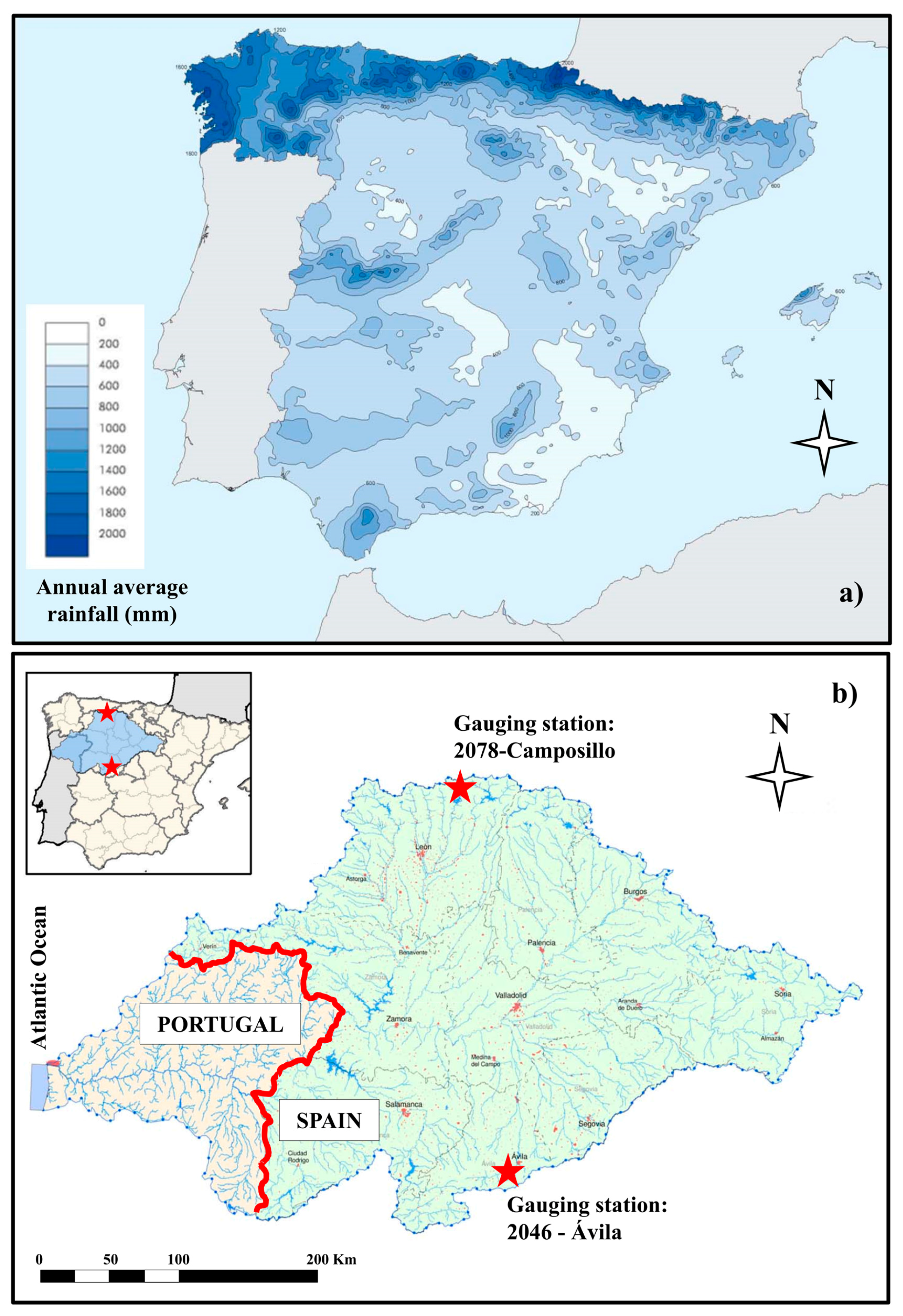
2.1. Study Areas

Water resources in Spain are characterized by an extreme variability, between the wet north, and the dry south. This has produced large irregularities among periods of droughts and rainfalls, as well as an increasing occurrence of extreme events (flooding and droughts), with an overall impact on the society [55].

In Spain, the rainfall distribution offers an irregular behavior, with a positive gradient with respect to latitude and southern asymmetry (Figure 1a). Furthermore, it increases with altitude and it is also closely linked to its strong orography.

Case studies are defined by gauging stations which are located upstream of the first regulating reservoirs. Consequently, these case studies comprise unregulated rivers stretches. The selection process was based on the annual average rainfall and rainfall variability north–south. Therefore, taking into account that annual average rainfall in Spain is 666 mm [56], two sub-basins were chosen (Figure 1b). First, in the Adaja sub-basin in the south, annual rainfall is lower than the average. Second, gauging station Ávila (code number 2046), the Porma sub-basin in the north, has an annual rainfall higher than the average. Gauging station Camposillo (code number 2078).

2.1.1. Adaja River

This case covers the whole upper basin of the Adaja river, also known as Ambles valley, where this river comprises the main riverbed. The study area occupies a central position within Iberian Peninsula with an area of 770.51 km², according to gauging station 2046-Avila.

Regarding climatic features, the zone is defined as cold Mediterranean, high continental, with moderately warm summers and severe winters. Mean annual temperature is 11 °C and the average annual rainfall is about 400 mm. Rainfall is presented as scarce and irregular. The key morphometric parametric are a main channel length of 47.09 km and a time of concentration of 13.58 h. Notice that the considered time of concentration is the legal requirement in Spain, which has the following formulation:

$$T_c=0.3·L_c·J_c^{-0.19}$$

(1)

where T_c is the time of concentration expressed in hours, L_c is the length of the main channel in kilometers, and J_c is the average slope of the main channel in meter/meter (dimensionless value).

2.1.2. Porma River

This basin is located in the northern and wet part of Spain. The analyzed area is placed in the southern slope of the Cantabrian range, in the north of the León province. The area of study, taking into account the gauging station 2078-Camposillo, has an extension of 140.16 km². From the hydrological point of view, Porma river is characterized by a pluvio-nival hydrological regime, with an annual average rainfall of around 1430 mm, and an average yearly temperature of 8.8 degrees Celsius (°C). From a morphometric point of view, the sub-basin is characterized by a main channel length of 17.99 km and a low time of concentration of about 5.24 h.

2.2. Data Description

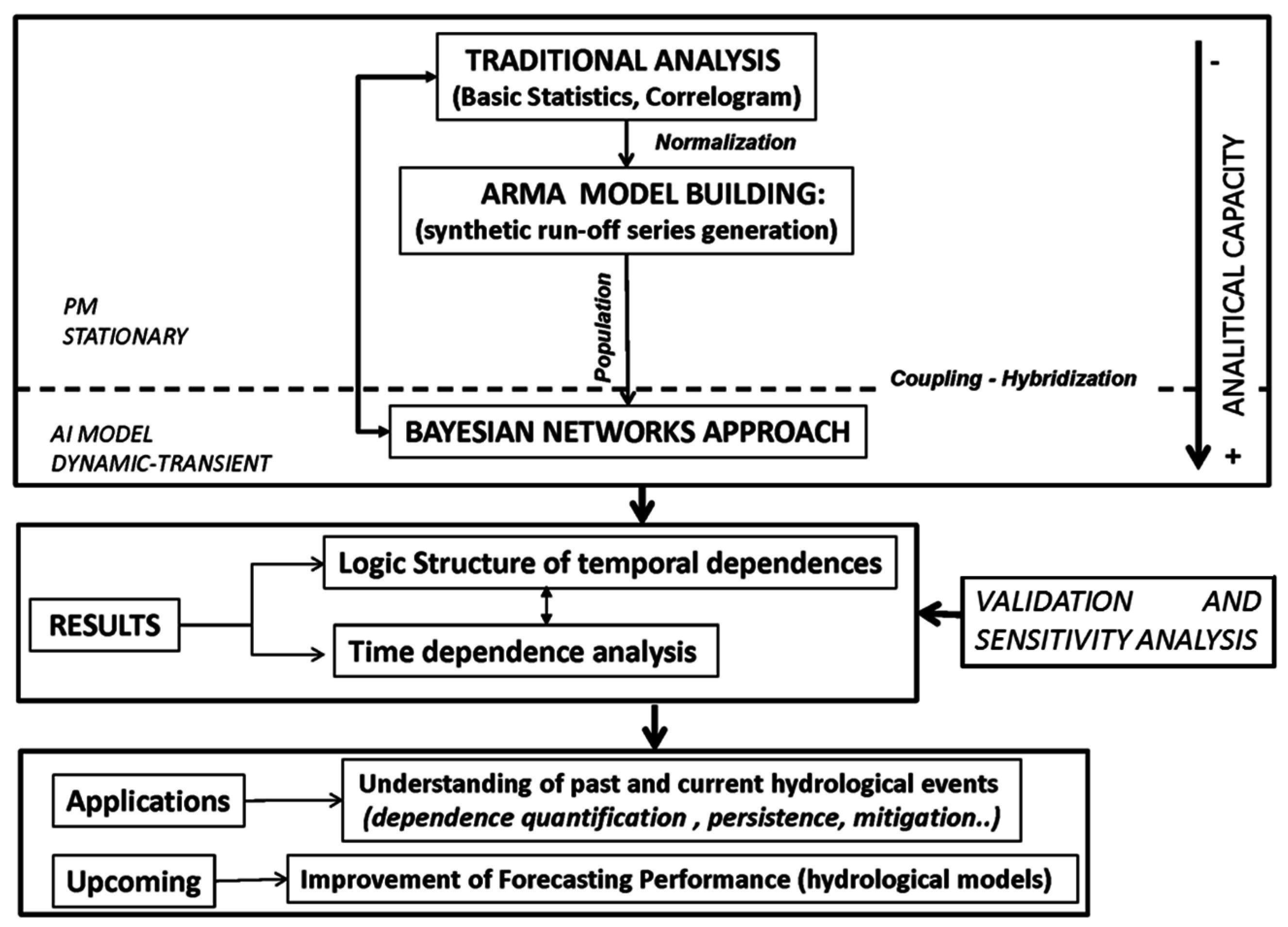
Annual runoff time series were obtained through the network of gauging stations belonging to Duero river basin Authority, the largest river basin in Iberian Peninsula. As the case studies are unrelated to each other, there are two different time periods of analysis for each sub-basin. In both cases, there are not missing data in the time series.

2.3. Methodology

The proposed methodology (Figure 2) starts with an analysis of basic statistics of the time series that also comprises the generation of correlograms. Then, an ARMA model was built to generate reliable equiprobable synthetic runoff series that populate the causal reasoning process. This was done through Bayes’s theorem that allowed the identification of the logic structure of a Bayesian Network (BN) that represents the complex relationships of time series temporal dependences. Synthetic series from the previous ARMA model populated the BNs. Finally, the right time order (model order) estimation for runoff series, obtained by BNs, was checked by a suitability identification of the time order by means of Risk Simulator software [57]. This analysis was developed considering the main criteria for appropriate model selection, such as Schwarz Criteria or Akaike Information Criterion, both based on Information Theory. However, the selection was made considering exclusively the Schwarz Criteria, because Akaike information Criteria tends to select higher time orders and less parsimonious models [58].

From a numeric point of view, Bayes’s theorem allows the calculation of the conditional probability. Consequently, prior (first time step) and posterior probability distributions of runoff for each time step (year) are generated at the population stage. A conditional probability statement is of the following type: if the variable B is in state b₁, then from either evidence or experience, we know that, as a result, the probability of the variable A in state a1, is x. The notation for this statement is:

$$P\left(a_1|b_1\right)=x$$

(2)

The expression P(A|B) denotes a Conditional Probability Table (CPT) containing numbers P(a_i|b_j). This probability distribution of B, written as P(B), together with the values given in the CPT can be used to calculate the resulting (a posteriori) probability distribution for P(A). To obtain this distribution BNs use the fundamental Bayes’s theorem.

$$P\left(B|A\right)=P\left(A|B\right)P\left(B\right)/P\left(A\right)$$

(3)

Here, the term P(A|B) is an expression of the joint probability for the variables A and B. Bayes’s theorem can be used to obtain the table P(B|A), which is the CPT showing the likely state of the variable B given the variable A, which is the reverse of the previous situation, also called back propagation of probability.

Furthermore, the resultant conditional probability permits the quantification of the relative percentage of annual runoff change, as well as providing the right time order of dependence. This approach is done time step by time step (dynamically), in contrast to other traditional approaches.

2.3.1. Stage 1. Traditional Time Analysis

First, a traditional time analysis, which mainly comprised basic statistics parameters, such as mean, standard deviation and variation and skewness coefficients, and a temporal correlation analysis through correlograms, was performed.

2.3.2. Stage 2. ARMA Model Building

It is well known that an Autoregressive Moving Average (ARMA) (p,q) is the extension of the AR model that uses two components to model the temporal correlation in time series.

An ARMA model comprises two components. The first component (p) is the autoregressive (AR) that uses a number of series delays. Consequently, p is the first term of an ARMA equation and represents the temporal dependence delay within a series. For instance, an annual series with p = 2 means that there are 2 years of temporal dependence. In other words, data depend on what happened up to 2 years earlier. The second component is the term (q) moving average (MA) that uses delays of the forecast errors to improve this process. Finally, an ARMA model is expressed as follows:

$$y_t=\mu +{\displaystyle \sum }_{j=1}^p{\theta }_j\left(y_{t-j}-\mu \right)+{\epsilon }_t-{\displaystyle \sum }_{j=1}^q{\theta }_j{\epsilon }_{t-j}$$

(4)

where μ is the mean of the time series, θ represents the correlation coefficient, y_t is the value of the temporal series at a certain time step j, q is the number of time steps and ε_t represents the historical residuals.

Generally, hydrological data are characterized by biased probability distributions that need to be normalized [26], because ARMA models assume Gaussian distributions for their variables [8,25]. This is made by normalizing functions but this is not enough to guarantee the normality. For this reason, and according to [25] (p. 93), the skewness test for normality was developed. The Skewness Coefficient test was applied to the historical series and both series (Adaja and Porma) show positive a skewness coefficient, outside the Snedecor and Cochran limits, for a confidence level of 95%, (the Adaja sub-basin: $1.23\notin \left[-0.56,0.56\right]$, the Porma sub-basin $0.98\notin \left[-0.75,0.75\right]$). Consequently, this test is negative which means that both series are not normal and they should be normalized for generating the ARMA models.

In order to take advantage of the BNs’ analytical potential, the generation of synthetic series were developed through a parsimonious ARMA (1,1) model. Given that BNs building requires that variables are connected consecutively, the analysis with the ARMA (1,1) model is appropriate because it is developed with the highest freedom degree. Thus, relationships among variables are not previously conditioned (“p” part of the ARMA model). Synthetic series were generated according to the general framework of [25]. All synthetic series have the same length as the historical records for each sub-basin. In order to avoid the boundary effect within ARMA modelling technical jargon, this generation process is called “non-conditioned”, in which a warm-up period of 20 years was established for both sub-basins.

The quality of the synthetic data generated by the ARMA models was assessed. This was done through the Kolmogorov–Smirnov–Lilliefors correction test, where goodness of fit between historical data and synthetic data was checked [59,60].

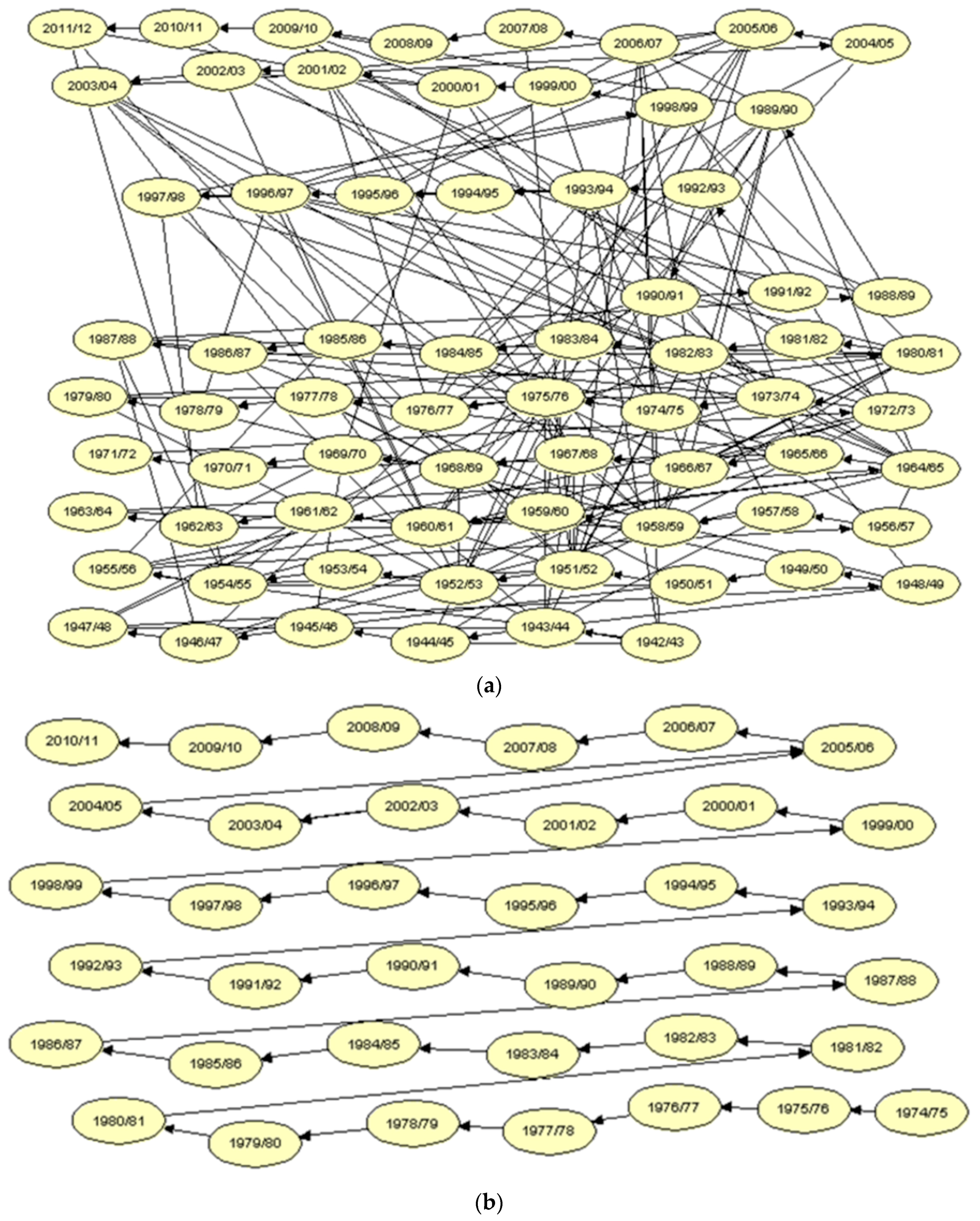
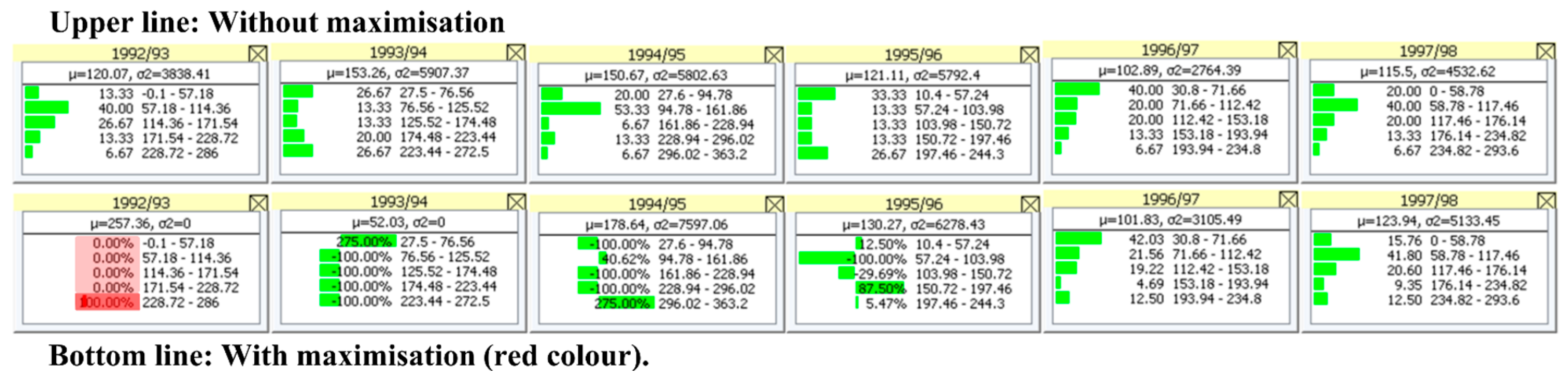
2.3.3. Stage 3. Bayesian Networks Building

The Bayesian approach is populated and trained from 200 synthetic annual runoff series that were previously generated through an ARMA model. The BN model automatically generates probabilistic distributions of runoff data for each year, as well as a logic structure, according to its internal dependences relationships (dependences and independences) in the data. This was done through Learning Wizard of HUGIN Expert (V 7.3).

This stage was started by building the logic structure that represents the complex temporal dependences between time steps (years) which are the decision variables within the BN. The dependence between consecutive years (Time Steps) seems obvious but the identification and assessment of time order dependences larger than one (non-consecutive years) is less trivial (Figure 3).

The logic structure is largely driven by the fact that each decision variable is assigned to each year of the respective data series. In this sense, BNs models comprise a set of variables, covering the whole period of the temporal series that interact year by year. The partition for every single variable was based on five intervals with the same range. Thus, Bayes’s theorem is propagated over time, using the conditional probability and calculating probability distributions for each year.

Figure 3 shows the logic structure for both basins where the noticeable independent nature of Adaja river basin’s temporal behavior is represented through the relationships among variables. Each arrow connecting non-consecutive years represents an independent relationship measured by a p-value. The p-value threshold is set at 0.1 which means that up to 10% of relationships of independence between decision variables are shown. It can also be seen that the complexity of independence connections is much higher for the Adaja sub-basin (a) than for the Porma sub-basin (b) for the same p-value threshold.

3. Results

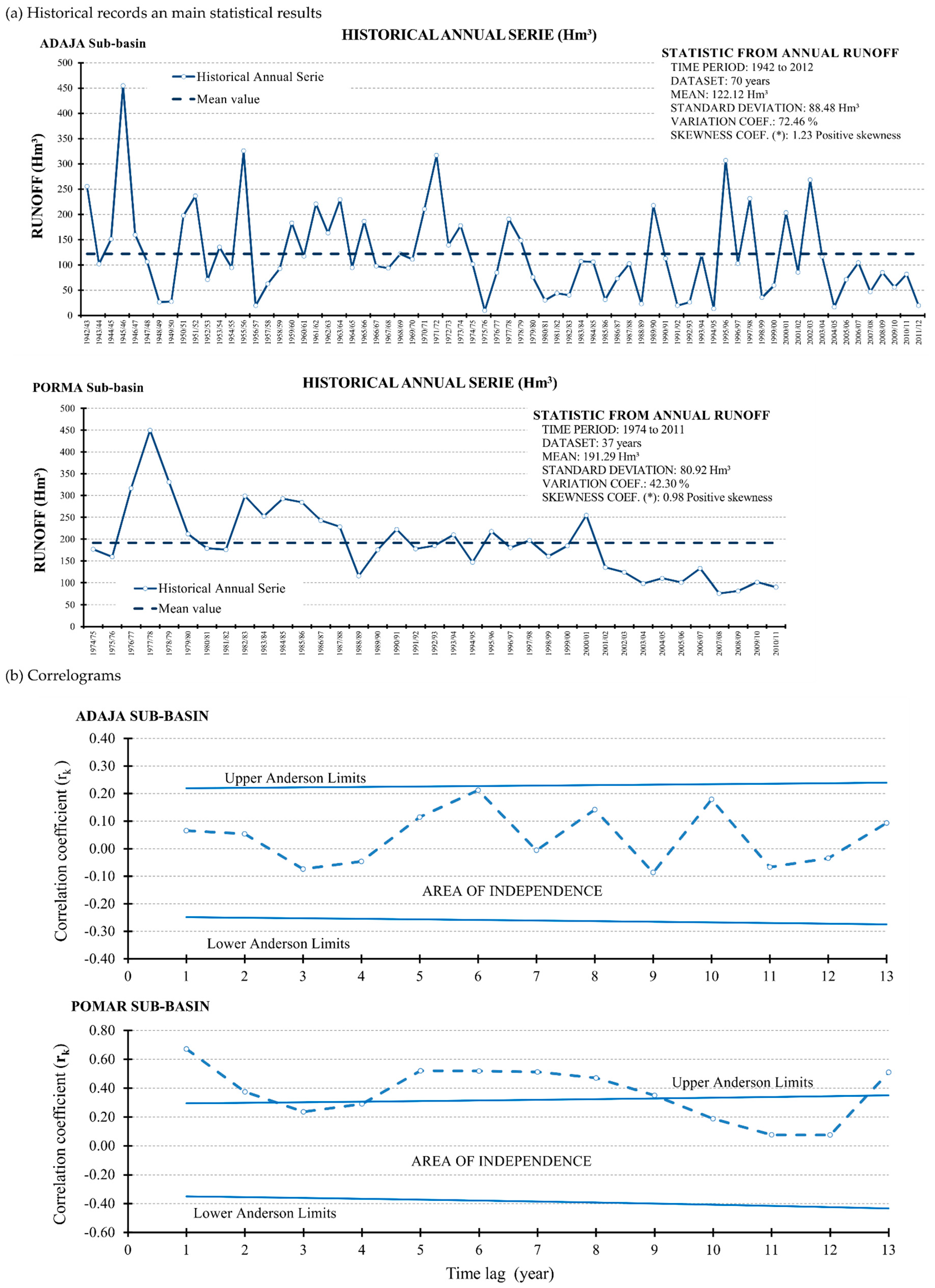
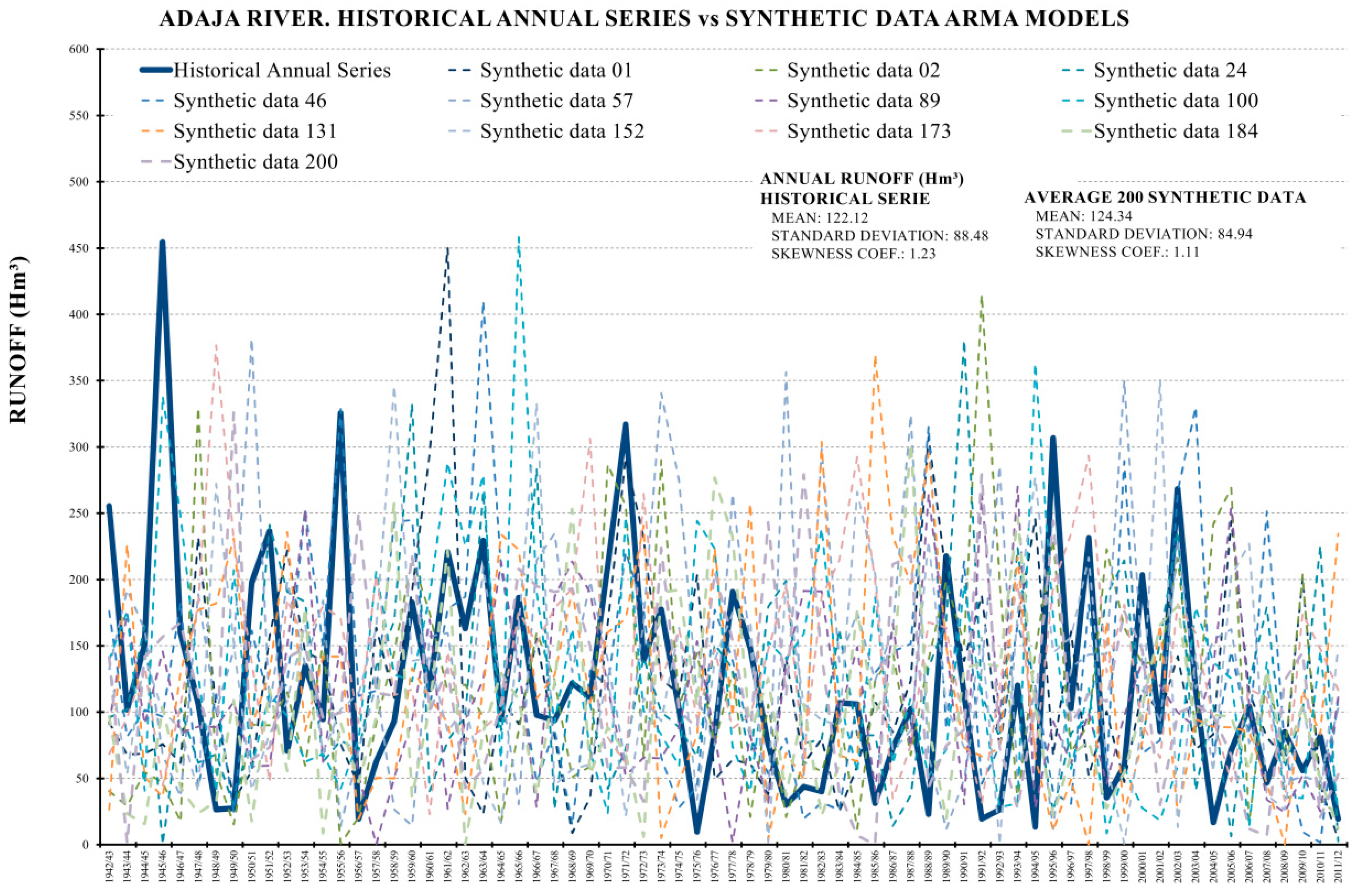
3.1. Traditional Time Analysis and Synthetic Series Prior Analyses

Figure 4a,b shows the main results drawn from the descriptive statistical analysis (Stage 1). This comprises a basic and prior stage for the subsequent BN development and analysis.

In the case of the Adaja sub-basin, all analyzed correlation coefficients (r_k = 1 to 13) are within Anderson limits which means that the series has a pure independent and continuous temporal behavior. In contrast, the Porma sub-basin correlation coefficients for certain time orders (lags) are outside Anderson limits which comprise variable or discontinuous dependence/independence behavior. The first lag interval reaches time lag 2, and it comprises a dependent behavior in the short term. Following lags (interval 5 to 9 and 13), shows a dependent and discontinuous behavior in the medium term. Both temporal behaviors should not be taken absolutely because the dependence/independence analysis through correlograms provides an average behavior and static analysis.

It is remarkable that the ARMA model preserved the main features of the historical series, such as mean and standard deviation (see

Table 1. Porma Sub-basin. (a) Goodness of fit results of synthetic series vs historical series made by Lilliefors corrected Kolmogorov–Smirnov test. Note: Test significance level (α) 5% (p-value). (*) Lilliefors significance correction. ** Lower bound of the true significance; (b) Autoregressive Moving Average Model (ARMA) models.

(a)	Porma Sub-Basins. Synthetic Series
Synthetic annual runoff series	01	02	07	18	27	62	94	104
Test Statistic	0.102	0.099	0.098	0.098	0.094	0.085	0.139	0.144
Asymp. Sig (2-tailed), p-value (*)	0.200 **	0.200 **	0.200 **	0.200 **	0.200 **	0.200 **	0.069	0.052
Synthetic annual runoff series	145	152	161	181	192	196	197	200
Test Statistic	0.101	0.139	0.101	0.126	0.139	0.072	0.103	0.115
Asymp. Sig (2-tailed), p-value (*)	0.200 **	0.069	0.200 **	0.147	0.069	0.200 **	0.200 **	0.200 **
(b)	Porma Sub-Basins. ARMA Models
Annual runoff series	01	02	07	18	27	62	94	104
Mean	173.85	186.84	205.07	182.69	169.84	243.98	203.08	223.99
Standard deviation	44.05	60.03	62.94	59.75	71.36	82.29	71.65	110.60
Skewness Coefficient	1.09	0.77	0.83	1.00	1.09	0.99	0.79	1.65
Annual runoff series	145	152	161	181	192	196	197	200
Mean	193.57	224.43	151.63	163.53	248.38	176.28	154.97	186.27
Standard deviation	49.51	101.10	50.49	63.23	105.83	83.20	53.64	75.93
Skewness Coefficient	0.86	0.96	0.99	0.91	1.30	0.80	0.89	1.21
	Average of All Annual Runoff Series				Historical Records
Mean	192.59				191.29
Standard deviation	74.66				80.92
Skewness Coefficient	0.88				0.98

and Figure 5). In order to analyze the goodness of fit of historical series and each synthetic series, a Kolmogorov–Smirnov–Lilliefors was developed. This test shows a very high goodness of fit. Furthermore, correlation coefficients of synthetic series preserve the same nature, regarding the temporal behavior, as the ones for historical series.

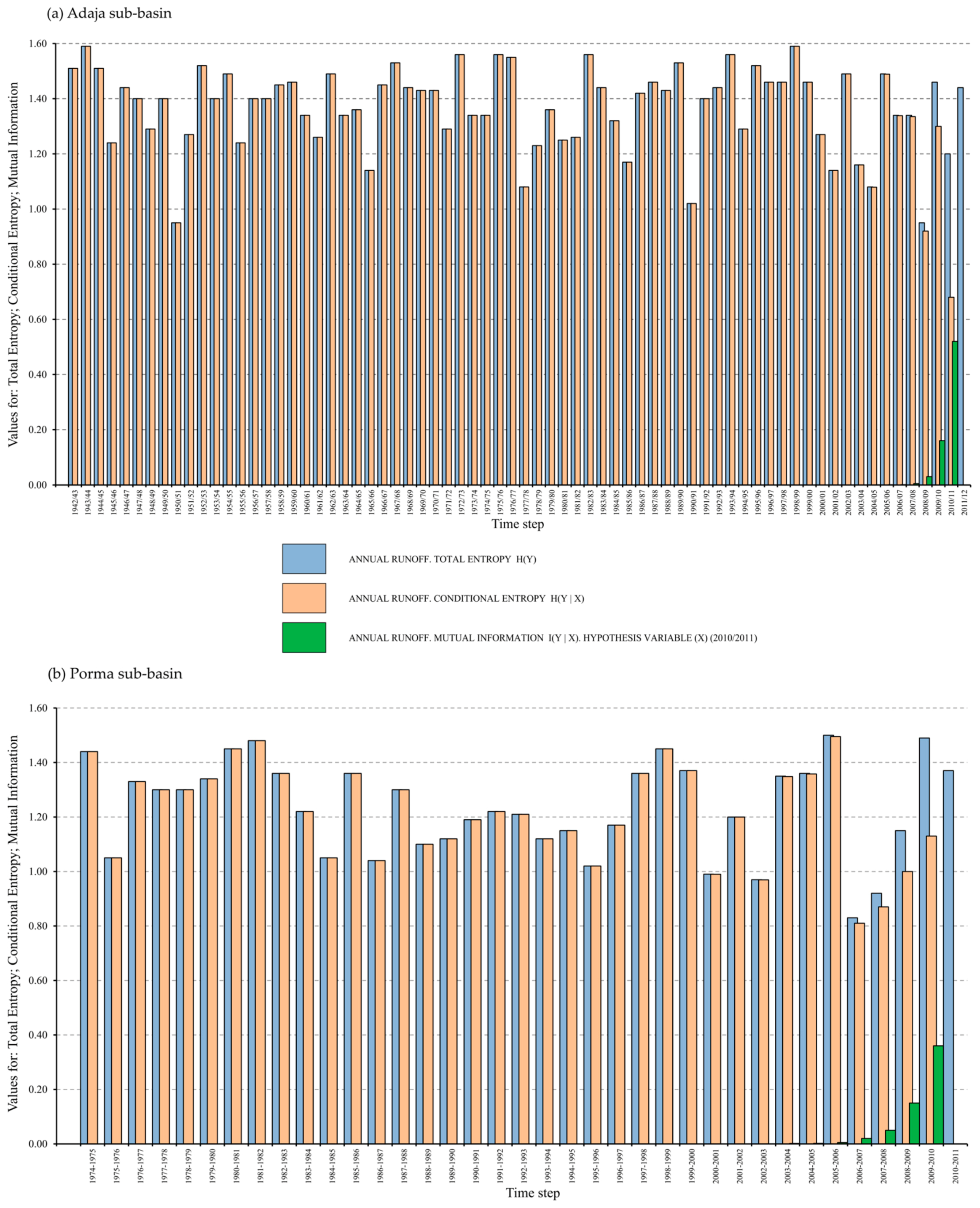
3.2. Hydrological Interpretation. Time Dependence Analysis

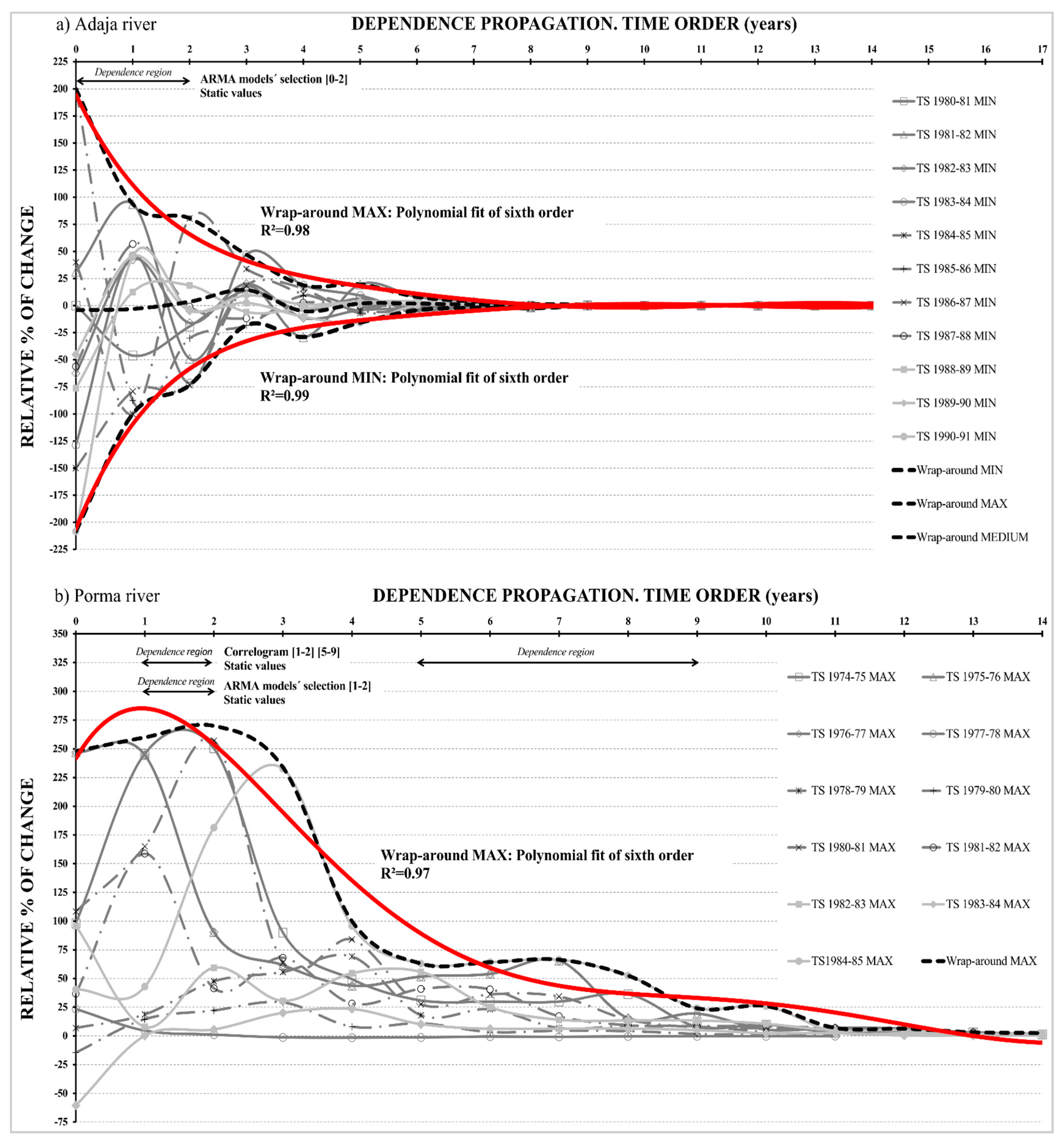
The temporal dependence analysis was developed through the relative percentage of runoff change estimation that a time step dynamically produces on the following ones. This was made in two ways. First, it was developed through the maximization of the highest interval of the probability distribution belonging to a year (Time Step) (Figure 6; maximization of the whole probability distribution); Second, it was developed by means of the analysis of the dependence propagation function (Figure 7; wrap-around MAX and MIN). In order to achieve a good understanding of this research methodology, results shown in Figure 7 should be seen as a whole, through the analysis of wrap-around MAX and MIN functions (wrap-around shapes).

3.2.1. Adaja River

In this case, the maximization of the highest intervals of probability distribution does not generate a logical or related impact on following years along the whole time period. This is demonstrated by the absence of a general common behavior or recognizable pattern on the influence that different time steps apply on the following ones (Figure 6). Therefore, time dependence analysis shows a pure independent temporal behavior.

On the other hand, as can be appreciated in Figure 7a, an analysis of the propagation function of dependence shows two wrap-around results. Here, the area under the wrap-around MAX (positive area) and the area above the wrap-around MIN (negative area) is essentially compensated (symmetric graph), which gives a total result of null temporal dependence. Furthermore, it is worth emphasizing that:

• Resulting symmetry on the shapes of wrap-around MAX and MIN practically coincides with the x-axis.
• Both wrap-around MAX and MIN tend (or decay) to zero rapidly (Figure 7a).
• There exists a very high goodness of fit of the shapes’ MAX and MIN of 0.98 and 0.99 respectively, measured by coefficient of determination R².
• This fit corresponds to a sixth order function for all time steps.

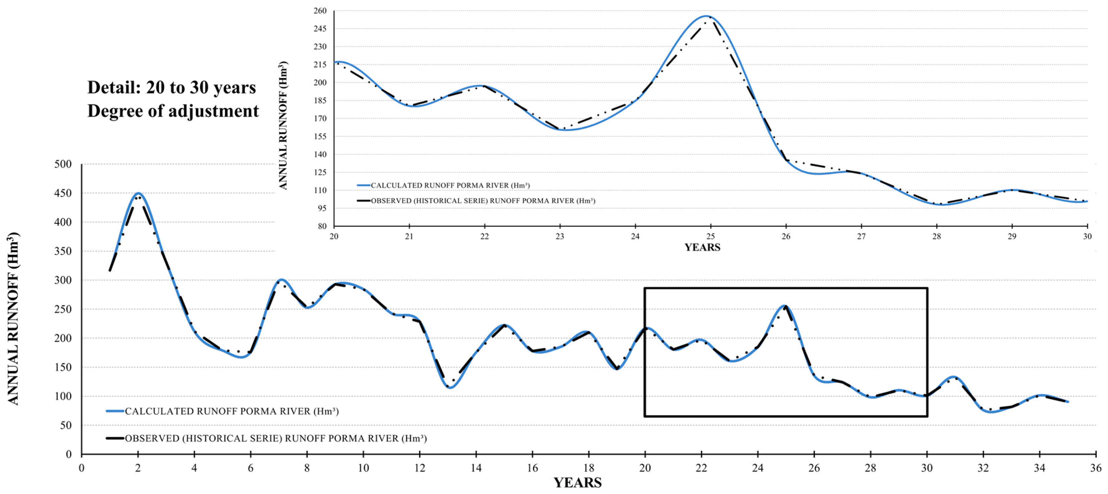
In this sense, the dynamic analysis of the dependence propagation (Figure 6 and Figure 7a) leads to an interpretation of the independent temporal behavior of time series which is from the beginning and is continuous. In contrast, the analysis carried out by the correlograms (Figure 4b) shows some cases (time lags 6 and 10) where the rk is very close to the limit and it can provide some doubts on the independent nature of the river basin. This different performance is due to the average result that the correlograms provide, in contrast to the dynamic and specific analysis that the BN provides.

3.2.2. Porma River

In this case, there is a non-insignificant variability on the change (dependence) that a particular time step applies on the following ones. According to the BN approach, dependence Time Order is placed in the range or region from 1 to 5 in the short-term (Figure 7b). The asymptotic behavior of the dependence over time is also remarkable. Here, the attenuation and convergence of all series in 0 takes place in a much longer time period than the previous case (Adaja river). This behavior of the time series could indicate an influence in the medium term.

Figure 7b shows that the wrap-around MAX (positive area) is clearly dominant, in contrast to the negative area which is practically null. Consequently, the distribution between positive and negative areas is not balanced (asymmetric graph). Furthermore, the shape and the high goodness of fit (R² = 0.97) of the wrap-around MAX (sixth order) for all time steps (Figure 7b) is significant. This shape is very representative of the general behavior of the analysis and it is the mathematical way to quantify and define the dependence. The fact that the dependence decay (mitigation) is not continuous (Figure 7b) is also remarkable. The dependence persistence and decay (mitigation) can be also observed in Figure 7b by analyzing the dependence behavior over time. In this sense, all series converge in 0 (y-axis), providing a very detailed way for the analysis of the dependence persistence-mitigation in the medium-term (13 years). A double dependence behavior can be clearly seen. Firstly, a continuous and rapid decay of dependence (or dependence mitigation from time order [1,2] up to time order 5. Secondly, a slight increase begins from time order 5 that smoothly concludes in time order 13. This continuous and differentiated behavior (from 1 up to 13) may indicate a temporal dependence, persistent in the short and medium term, which is not detected by a correlogram (see Figure 4b, independent behavior in the intervals [3,4] and [10,11,12]). However, in a correlogam, there is also a lag (Time order) range where dependence raises between lags 5 and 9, as shown in Figure 4b, that noticeably coincides with a slight raise in dependence analysis though the BN approach (Figure 7b).

On the other hand, in this case study, there are also two points of indeterminacy in the correlograms analysis. The first one is for time lag 4 and the second one for time lag 9. In both of them, the indeterminacy may be caused by the same aforementioned reasons as in the Adaja case study. The analysis of dependence propagation removes these indeterminacy points, improving and deepening the knowledge of temporal behavior of a hydrological series.

3.3. Time Order (Model Orden) Suitability Analysis

A suitability analysis of different time orders’ ARMA models was done by means of Risk Simulator software [57]. This should be taken as another way of validating the calculated results via BN models.

Table 2. Suitability identification of time order through ARMA modelling. Note: Results ordered according to Schwarz Criteria.

Sub-Basins	ARMA Model	Schwarz Criteria	Akaike Information Criteria
Adaja	p = 0, q = 1	11.792	11.669
	p = 1, q = 1	11.981	11.795
	p = 2, q = 0	12.083	11.895
	p = 1, q = 0	12.245	12.121
	p = 0, q = 2	12.580	12.394
	p = 2, q = 0	12.764	12.573
Porma	p = 2, q = 0	11.025	10.720
	p = 0, q = 2	11.026	10.733
	p = 2, q = 2	11.206	10.698
	p = 1, q = 0	11.224	11.025
	p = 1, q = 1	11.308	11.010

shows the main results for each case study. Furthermore,

Table 3. Comparison of time order suitability analysis from applied techniques. (*) Static (**) Dynamic.

Sub-Basins	Technique
	Correlogram (*)	BNs (**)	Suitability Analysis. “p” Part of ARMA Models (*)
Adaja	Full independent	0 (Independent)	[0–2] (*)
Porma	[1–2] and [5–9] Discontinuous dependent behavior	[0–13] Continuous dependent behavior	[1–2] (*) Particular dependent behavior

summarizes the time order suitability analysis from the different techniques. The ARMA models’ selection through Risk Simulator software agrees with the BNs’ approach results. In this sense, for the Adaja sub-basin, the ARMA model that best fits the indicates that the temporal basin behavior is independent. In fact, the ARMA model that fits better is ARMA (0,1). On the other hand, for the Porma river basin, this analysis provides a selection of models where the right time order is around 2, which coincides with the analysis from the BN in the short term. Due to the aforementioned technical reasons and to the fact of letting the temporal analysis have the maximum freedom, decision variables should be connected consecutively in BN building. Consequently, the ARMA models built for Adaja and Porma rivers were ARMA (1,1). Temporal behavior of the runoff series in the medium term cannot be validated through ARMA models’ selection. Consequently, in order to analyze the internal coherence of temporal behavior in the medium term, an analysis of all series for each river basin was developed. As more equiprobable data series are available, this analysis becomes a more useful way to check the internal coherence of a temporal behavior data series.

Table 2 shows a summary of the results (temporal dependence behavior) obtained from all applied techniques.

3.4. Consistency and Quality Assessment of the BNs Model and Its Analysis

After developing the model’s structure, estimating the conditional probabilities and getting the results, the BN and its analysis needs to be evaluated. Given that this is a pure quantitative BN model, its evaluation should include assessments of predictive accuracy and sensitivity analysis. Predictive accuracy refers to a quantitative evaluation of the model, by comparing model predictions with observed data [62].

Capturing and reproducing the real behavior patterns of temporal hydrological series is a crucial issue for prediction. This was developed by means of the comparison of the results drawn from BNs versus raw runoff observed data, directly drawn from gauging stations. Thus, the internal consistency and quality of this causal analysis is tested in the short and medium term. Figure 8 shows the results for Porma river. In order to obtain comparable information between both ways, probabilistic distributions were converted into deterministic data by means of multiplying the dependence among variables $\left(1-p_{value}\right)$ by the corresponding historical value (datum from gauge station).

This is expressed in general terms as:

$${\left[Deterministi{c}_{value}\right]}_{tlag{}_y}^{tla{g}_{y-n}}={\left[\left(1-p_{value}\right)\right]}_{tla{g}_i}^{tla{g}_{i-n}}·HS$$

(5)

where $\left(1-p_{value}\right)$ is the dependence rate, HS is the historical value, y represents the considered year, and n is the number of years from the year used to calculate the series’ beginning.

The fact that this method is able to reproduce so accurately a single time series, after raw gauge stations data had passed through several stages (basic statistic study, generation of synthetic series through ARMA model and generation of BN model), makes the whole approach much more robust and reliable as well as validating the whole process.

Sensitivity analysis can be performed using two types of measures: entropy and Shannon’s measure of mutual information [50]. The entropy measure is based on the assumption that the uncertainty or randomness of a variable X, characterized by probability distribution P(x), can be represented by the entropy function H(X):

$$H\left(X\right)=-{\displaystyle \sum }_{x\notin X}P\left(x\right)logP\left(x\right)$$

(6)

Entropy of a probability distribution can be defined as a measure of the associated uncertainty to that random process that this distribution describes. Consequently, a score of the uncertainty/certainty level of events can be made attending to this entropy, H(X).

Reducing H(X) by collecting information, in addition to the current knowledge about the variable X, is interpreted as reducing the uncertainty about the true state of X [63]. The entropy measure therefore enables an assessment of the additional information required to specify a particular alternative. Shannon’s measure of mutual information is used to assess the effect of collecting information about one variable (Y) on reducing the total uncertainty about variable X, using:

$$I\left(Y.X\right)=H\left(Y\right)-H(Y\mid \mathrm{X})$$

(7)

where $I\left(Y.X\right)$ is the mutual information between variables. This measure reports the expected degree to which the joint probability of X and Y diverges from what it would be if X were independent of Y. If $I\left(Y.X\right)=0$, X and Y are mutually independent [50].

$H(Y\mid X)$ is conditional entropy which means the uncertainty that remains about Y, when X is known to be x.

This has been very useful in this research because the temporal dependence analysis, shown in Figure 7 (Section 3.2), has been satisfactorily compared with this analysis. The fact that two variables, that represent the annual runoff of two years, have a mutual information ≠ 0 shows that they are dependent [50]. On the contrary, in that case that the mutual information is 0, they are independent. This analysis represents another way for characterizing and quantifying the temporal dependence and behavior of a hydrological series.

An assessment of the entropy associated to each variable, the conditional entropy and mutual information for each variable and connection were developed for Adaja and Porma rivers using HUGIN expert software (Figure 9). This analysis reasonably agrees with the analysis and results interpretation developed in Section 3.2. Thus, Porma river presents around 13–14 years (time lag) where mutual information is not cero and consequently, variables are, to some extent, dependent. The fact that this time lag coincides with the dependence temporal analysis shown in Figure 7 is remarkable. For the Adaja river basin, this analysis also coincides with the previous analysis and the time lag of non-null mutual information is around 9 years. It is important to make clear that, given the extremely low values of the mutual information for the Adaja river basin, this result does not invalidate the conclusion about its independent nature.

A sensitivity analysis of this BN is made by means of the assessment of Total Entropy, which, in turn, is the summation of Mutual Information and Conditional Entropy (Figure 9). If two variables that represent the annual runoff of two years have a mutual information = 0, they are independent. In other words, they are not temporally connected. On the contrary, if the mutual information is ≠ 0, this means that they are dependent. In Figure 9, blue bars represent the value for Total Entropy, orange bars represent the value for Conditional Entropy and green bars represent the value for Mutual Information. Notice that those time steps that are independent have the same value for Total Entropy and Conditional Entropy, and the value for Mutual information is cero. On the other hand, when there is some dependence between time steps, there is a non-null value for mutual information.

4. Discussion and Conclusions

Causality and conditional probability has been demonstrated in this research to be very useful in the analysis of the temporal behavior of runoff series. According to the new tendencies on hydrological research, BNs can be hybridized or coupled with traditional techniques, providing the engineer and scientist with robust and powerful tools. Due to the aforementioned BNs’ properties, this technique can be categorized within the Artificial Intelligent discipline.

Traditional techniques such as a correlogram, PM and NP models have been extensively used over the last decades. The application of BNs for hydrological temporal analysis has been demonstrated to be suitable due to the following reasons. First, the inherent uncertainty/randomness of hydrological processes is well captured and assessed by this technique, because apart from the definition of probability distributions with their basic statistics, several tests (Entropy, Mutual Information, Conditional Entropy, p-value, $1-p_{value}$), belonging to Information Theory, can be applied; second, the dynamic nature of temporal analysis is properly incorporated because of the flexibility and modularity of BNs; and finally, recent observed increasing variability in hydrological patterns could be much more properly analyzed and incorporated through BNs because the real knowledge increases.

Furthermore, another advantage is the fact that BNs’ application does not require that the relationships between model variables are defined mathematically before establishing the analysis. BNs, through Bayesian observational inference via the Bayesian theorem, calculate prior and posterior probability functions. This advantage ensures that the performance working with non-stationary hydrological time series is much more accurate.

On the other hand, it is known that a correlogram comprises a static picture and average result of the temporal behavior of a hydrological series. This fact provokes the existence of indeterminacy points when it comes to defining the temporal dependence/independence of time series (see Section 3.1 and Figure 4b). In this sense, BNs have allowed, by means of the dynamic and specific analysis of the temporal dependences, time step by time step, the removal of this indeterminacy (Figure 4b). This is possible because the attention can be focused on a particular time step and this provides a more accurate analysis. Furthermore, the dynamic analysis that causal reasoning delivers allows quantifying and establishing thresholds of dependence relationships (Figure 3).

Furthermore, the BNs’ application has allowed the detection of non-trivial dependence relationships (time lag >1). Also, the analytical potential of BNs has been demonstrated when the functions for propagation of the dependence were defined (Figure 7). Consequently, from parsimonious and non-conditioned ARMA (1,1) models that populated and trained the BNs, dependence of relationships was detected in the short and medium term.

Causality and conditional probability through BNs is aimed here to assess the influence of time (time step) on the rest of the time series (rest of time steps). Therefore, every year (time step) becomes a decision variable into the BNs system. It is remarkable that, within the BN, a little change in the probabilities of runoff can condition or affect a great runoff volume, corresponding to following years. This is very useful and novel because it allows the assessment of the dependence persistence and/or the dependence propagation (mitigation or attenuation) of a series, by means of analyzing the intensity of probability propagation. Likewise, it is possible to assess the dependence of one time step on the previous ones through the back-probability propagation, in other words, past information will provide prior knowledge of the future.

Consequently, this pure quantitative BN model becomes a predictive model for forecasting purposes. Its evaluation includes assessments of predictive accuracy and sensitivity analysis. Predictive accuracy refers to a quantitative evaluation of the model, by comparing model predictions with observed data. On the other hand, sensitivity analysis was carried out through the assessment of the Entropy and Mutual information of each decision variable. Thus, the internal consistency and quality of this causal analysis is tested.

It is also necessary to remark the reasonable coherence in the short-term between time orders obtained from a correlogram, suitability analysis via ARMA models and the one obtained through BNs. Additionally, the main contribution of this approach is that it allows the assessment of the temporal dependence in the medium term. This is an innovation over traditional techniques where the short term can be assessed by means of a correlogram and ARMA models, and the long term can be evaluated through Hurst coefficient.

Dependence quantification is a concept that has not been sufficiently studied. It is well known that a correlogram provides an idea of temporal dependence intensity through the correlation coefficient. However, it seems necessary to have tools that allow the quantification of that dependence more accurately. Causal reasoning through BNs allows the quantification of that dependence for every single time step of a hydrological series. In this sense, upcoming research studies will aim to provide a sort of indicator of the rate of dependence for different river basins. Of course, this rate will be dynamic as it will change as the series develops over time. This dependence rate might be expressed in Hm³ units for annual runoff series. Consequently, this could provide a useful technique, primarily for water management, because it would improve the knowledge on the water resources’ availability in a river basin. Furthermore, it would generate more accurate information in order to achieve a better planning and dimensioning of water infrastructures, especially in unregulated rivers, for instance, in the optimization of reservoir operation rules. All of this would lead to defining more realistic water management scenarios. Future research lines will also aim to generate stochastic forecast or predictive models through identifying and quantifying patterns of change, as well as identifying and solving the functions that drive the dependence of a certain series, considering the uncertainty.

Integrated and sustainable water management demands approaches such as causal reasoning-BNs that improve existing knowledge and enhance the analytic capacity.

References

1. Reihan, A.; Kriauciuniene, J.; Meilutyte-Barauskiene, D.; Kolcova, T. Temporal Variation of Spring Flood in Rivers of the Baltic States. Hydrol. Res. 2012, 43, 301–314. [Google Scholar] [CrossRef]
2. Yang, C.; Yu, Z.; Hao, Z.; Zhang, J.; Zhu, J. Impact of Climate Change on Flood and Drought Events in Huaihe River Basin, China. Hydrol. Res. 2012, 43, 14–22. [Google Scholar] [CrossRef]
3. Pulido-Velazquez, D.; Luis Garcia-Arostegui, J.; Molina, J.; Pulido-Velazquez, M. Assessment of Future Groundwater Recharge in Semi-Arid Regions under Climate Change Scenarios (Serral-Salinas Aquifer, SE Spain). Could Increased Rainfall Variability Increase the Recharge Rate? Hydrol. Process. 2015, 29, 828–844. [Google Scholar] [CrossRef]
4. Bogner, K.; Liechti, K.; Zappa, M. Post-Processing of Stream Flows in Switzerland with an Emphasis on Low Flows and Floods. Water 2016, 8, 115. [Google Scholar] [CrossRef]
5. Hurst, H.E. Long-Term Storage Capacity of Reservoirs. Trans. Am. Soc. Civ. Eng. (ASCE) 1951, 116, 770–808. [Google Scholar]
6. Box, G.E.; Jenkins, G.M. Time Series Analysis: Forecasting and Control; Holden-Day: San Francisco, CA, USA, 1976; p. 575. [Google Scholar]
7. Akintug, B.; Rasmussen, P.F. A Markov Switching Model for Annual Hydrologic Time Series. Water Resour. Res. 2005, 41, W09424. [Google Scholar] [CrossRef]
8. Kim, T.W.; Valdes, J.B. Synthetic Generation of Hydrologic Time Series Based on Nonparametric Random Generation. J. Hydrol. Eng. 2005, 10, 395–404. [Google Scholar] [CrossRef]
9. Stojkovic, M.; Prohaska, S.; Plavsic, J. Stochastic Structure of Annual Discharges of Large European Rivers. J. Hydrol. Hydromech. 2015, 63, 63–70. [Google Scholar] [CrossRef]
10. Andreu, J. Capítulo 1: Reflexiones sobre la planificación hidrológica. In Conceptos y Métodos Para la Planificación Hidrológica, 1st ed.; Sauquillo Herraiz, A., Ed.; Centro Internacional de Métodos Numéricos en Ingeniería (CIMNE): Barcelona, Spain, 1993; pp. 2–3. [Google Scholar]
11. Wang, W.; Chau, K.; Cheng, C.; Qiu, L. A Comparison of Performance of several Artificial Intelligence Methods for Forecasting Monthly Discharge Time Series. J. Hydrol. 2009, 374, 294–306. [Google Scholar] [CrossRef]
12. Romano, E.; del Bon, A.; Petrangeli, A.B.; Preziosi, E. Generating Synthetic Time Series of Springs Discharge in Relation to Standardized Precipitation Indices. Case Study in Central Italy. J. Hydrol. 2013, 507, 86–99. [Google Scholar] [CrossRef]
13. Díaz Caballero, F.F. Selección de Modelos Mediante Criterios de Información en Análisis Factorial: Aspectos Teóricos y Computacionales; Granada University: Granada, Spain, 2011; p. 28. [Google Scholar]
14. Todini, E. History and Perspectives of Hydrological Catchment Modelling. Hydrol. Res. 2011, 42, 73–85. [Google Scholar] [CrossRef]
15. Myung, I.J. The Importance of Complexity in Model Selection. J. Math. Psychol. 2000, 44, 190–204. [Google Scholar] [CrossRef] [PubMed]
16. Kendall, D.R.; Dracup, J.A. A Comparison of Index-Sequential and Ar(1) Generated Hydrologic Sequences. J. Hydrol. 1991, 122, 335–352. [Google Scholar] [CrossRef]
17. Lin, G.F.; Lee, F.C. Assessment of Aggregated Hydrologic Time-Series Modeling. J. Hydrol. 1994, 156, 447–458. [Google Scholar] [CrossRef]
18. Zhao, X.; Chen, X. Auto Regressive and Ensemble Empirical Mode Decomposition Hybrid Model for Annual Runoff Forecasting. Water Resour. Manag. 2015, 29, 2913–2926. [Google Scholar] [CrossRef]
19. Burlando, P.; Rosso, R.; Cadavid, L.G.; Salas, J.D. Forecasting of Short-Term Rainfall using ARMA Models. J. Hydrol. 1993, 144, 193–211. [Google Scholar] [CrossRef]
20. Karthikeyan, L.; Kumar, D.N. Predictability of Nonstationary Time Series using Wavelet and EMD Based ARMA Models. J. Hydrol. 2013, 502, 103–119. [Google Scholar] [CrossRef]
21. Mohammadi, K.; Eslami, H.R.; Kahawita, R. Parameter Estimation of an ARMA Model for River Flow Forecasting using Goal Programming. J. Hydrol. 2006, 331, 293–299. [Google Scholar] [CrossRef]
22. Salas, J.D. Analysis and modeling of hydrologic time series. In The McGraw Hill Handbook of Hydrology, 1st ed.; Maidment, D.R., Ed.; McGraw-Hill: New York, NY, USA, 1993; Chapter 19; pp. 1–72. [Google Scholar]
23. Salas, J.D.; Boes, D.C.; Smith, R.A. Estimation of ARMA Models with Seasonal Parameters. Water Resour. Res. 1982, 18, 1006–1010. [Google Scholar] [CrossRef]
24. Nourani, V.; Kisi, O.; Komasi, M. Two Hybrid Artificial Intelligence Approaches for Modeling Rainfall-Runoff Process. J. Hydrol. 2011, 402, 41–59. [Google Scholar] [CrossRef]
25. Salas, J.; Delleur, J.; Yevjevich, V.; Lane, W.L. Applied Modeling of Hydrologic Time Series, 1st ed.; Water Resources Publications: Littleton, CO, USA, 1980; p. 484. [Google Scholar]
26. Lee, T.; Salas, J.D.; Prairie, J. An Enhanced Nonparametric Streamflow Disaggregation Model with Genetic Algorithm. Water Resour. Res. 2010, 46, W08545. [Google Scholar] [CrossRef]
27. Vogel, R.M.; Shallcross, A.L. The Moving Blocks Bootstrap versus Parametric Time Series Models. Water Resour. Res. 1996, 32, 1875–1882. [Google Scholar] [CrossRef]
28. Srinivas, V.V.; Srinivasan, K. Hybrid Moving Block Bootstrap for Stochastic Simulation of Multi-Site Multi-Season Streamflows. J. Hydrol. 2005, 302, 307–330. [Google Scholar] [CrossRef]
29. Srivastav, R.K.; Srinivasan, K.; Sudheer, K.P. Simulation-Optimization Framework for Multi-Season Hybrid Stochastic Models. J. Hydrol. 2011, 404, 209–225. [Google Scholar] [CrossRef]
30. Ouarda, T.B.M.J.; Labadie, J.W.; Fontane, D.G. Indexed Sequential Hydrologic Modeling for Hydropower Capacity Estimation. J. Am. Water Resour. Assoc. 1997, 33, 1337–1349. [Google Scholar] [CrossRef]
31. Sharma, A.; Tarboton, D.G.; Lall, U. Streamflow Simulation: A Nonparametric Approach. Water Resour. Res. 1997, 33, 291–308. [Google Scholar] [CrossRef]
32. Lall, U.; Sharma, A. A Nearest Neighbor Bootstrap for Resampling Hydrologic Time Series. Water Resour. Res. 1996, 32, 679–693. [Google Scholar] [CrossRef]
33. Rajagopalan, B.; Salas, J.D.; Lall, U. Stochastic methods for modeling precipitation and streamflow. In Advances in Data-Based Approaches for Hydrologic Modeling and Forecasting; Berndtsson, R., Sivakumar, B., Eds.; World Scientific: Singapore, 2010; Chapter 2; pp. 17–52. [Google Scholar]
34. Adarnowski, J.F. Development of a Short-Term River Flood Forecasting Method for Snowmelt Driven Floods Based on Wavelet and Cross-Wavelet Analysis. J. Hydrol. 2008, 353, 247–266. [Google Scholar] [CrossRef]
35. Zounemat-Kermani, M.; Teshnehlab, M. Using Adaptive Neuro-Fuzzy Inference System for Hydrological Time Series Prediction. Appl. Soft Comput. 2008, 8, 928–936. [Google Scholar] [CrossRef]
36. Aqil, M.; Kita, I.; Yano, A.; Nishiyama, S. A Comparative Study of Artificial Neural Networks and Neuro-Fuzzy in Continuous Modeling of the Daily and Hourly Behaviour of Runoff. J. Hydrol. 2007, 337, 22–34. [Google Scholar] [CrossRef]
37. Molina, J.; Pulido-Velazquez, D.; Luis Garcia-Arostegui, J.; Pulido-Velazquez, M. Dynamic Bayesian Networks as a Decision Support Tool for Assessing Climate Change Impacts on Highly Stressed Groundwater Systems. J. Hydrol. 2013, 479, 113–129. [Google Scholar] [CrossRef]
38. Chan, T.U.; Hart, B.T.; Kennard, M.J.; Pusey, B.J.; Shenton, W.; Douglas, M.M.; Valentine, E.; Patel, S. Bayesian Network Models for Environmental Flow Decision Making in the Daly River, Northern Territory, Australia. River Res. Appl. 2012, 28, 283–301. [Google Scholar] [CrossRef]
39. Molina, J.L.; Bromley, J.; Garcia-Arostegui, J.L.; Sullivan, C.; Benavente, J. Integrated Water Resources Management of Overexploited Hydrogeological Systems using Object-Oriented Bayesian Networks. Environ. Model. Softw. 2010, 25, 383–397. [Google Scholar] [CrossRef]
40. Mamitimin, Y.; Feike, T.; Doluschitz, R. Bayesian Network Modeling to Improve Water Pricing Practices in Northwest China. Water 2015, 7, 5617–5637. [Google Scholar] [CrossRef]
41. Castelletti, A.; Soncini-Sessa, R. Bayesian Networks and Participatory Modelling in Water Resource Management. Environ. Model. Softw. 2007, 22, 1075–1088. [Google Scholar] [CrossRef]
42. Henriksen, H.J.; Barlebo, H.C. Reflections on the use of Bayesian Belief Networks for Adaptive Management. J. Environ. Manag. 2008, 88, 1025–1036. [Google Scholar] [CrossRef] [PubMed]
43. Malekmohammadi, B.; Kerachian, R.; Zahraie, B. Developing Monthly Operating Rules for a Cascade System of Reservoirs: Application of Bayesian Networks. Environ. Model. Softw. 2009, 24, 1420–1432. [Google Scholar] [CrossRef]
44. Varis, O.; Fraboulet-Jussila, S. Water Resources Development in the Lower Senegal River Basin: Conflicting Interests, Environmental Concerns and Policy Options. Int. J. Water Resour. Dev. 2002, 18, 245–260. [Google Scholar] [CrossRef]
45. Bennett, J.C.; Wang, Q.J.; Pokhrel, P.; Robertson, D.E. The Challenge of Forecasting High Streamflows 1–3 Months in Advance with Lagged Climate Indices in Southeast Australia. Nat. Hazards Earth Syst. Sci. 2014, 14, 219–233. [Google Scholar] [CrossRef] [Green Version]
46. Pokhrel, P.; Robertson, D.E.; Wang, Q.J. A Bayesian Joint Probability Post-Processor for Reducing Errors and Quantifying Uncertainty in Monthly Streamflow Predictions. Hydrol. Earth Syst. Sci. 2013, 17, 795–804. [Google Scholar] [CrossRef]
47. Aviles, A.; Celleri, R.; Solera, A.; Paredes, J. Probabilistic Forecasting of Drought Events using Markov Chain- and Bayesian Network-Based Models: A Case Study of an Andean Regulated River Basin. Water 2016, 8, 37. [Google Scholar] [CrossRef]
48. Wang, Q.J.; Robertson, D.E.; Chiew, F.H.S. A Bayesian Joint Probability Modeling Approach for Seasonal Forecasting of Streamflows at Multiple Sites. Water Resour. Res. 2009, 45, W05407. [Google Scholar] [CrossRef]
49. Zhao, T.; Wang, Q.J.; Bennett, J.C.; Robertson, D.E.; Shao, Q.; Zhao, J. Quantifying Predictive Uncertainty of Streamflow Forecasts Based on a Bayesian Joint Probability Model. J. Hydrol. 2015, 528, 329–340. [Google Scholar] [CrossRef]
50. Pearl, J. Probabilistic Reasoning in Intelligent Systems: Networks of Plausible Inference; Morgan Kaufmann: San Francisco, CA, USA, 1988. [Google Scholar]
51. Jensen, F.V. An Introduction to Bayesian Networks; UCL Press: London, UK, 1996. [Google Scholar]
52. See, L.; Openshaw, S. A Hybrid Multi-Model Approach to River Level Forecasting. Hydrol. Sci. J. 2000, 45, 523–536. [Google Scholar] [CrossRef]
53. Sang, Y.; Shang, L.; Wang, Z.; Liu, C.; Yang, M. Bayesian-Combined Wavelet Regressive Modeling for Hydrologic Time Series Forecasting. Chin. Sci. Bull. 2013, 58, 3796–3805. [Google Scholar] [CrossRef]
54. Jain, A.; Kumar, A.M. Hybrid Neural Network Models for Hydrologic Time Series Forecasting. Appl. Soft Comput. 2007, 7, 585–592. [Google Scholar] [CrossRef]
55. MAGRAMA. 2016. Available online: http://www.magrama.gob.es/es/agua/temas/seguridad-de-presas-y-embalses/desarrollo (accessed on 11 November 2015).
56. MAGRAMA. 2016. Available online: http://sig.magrama.es/saih/ (accessed on 14 August 2016).
57. Mun, J. Modeling Risk: Applying Monte Carlo Risk Simulation, Strategic Real Options, Stochastic Forecasting, and Portfolio Optimization; John Wiley & Sons: Hoboken, NJ, USA, 2010. [Google Scholar]
58. Peña, D. Análisis de Series Temporales; Alianza Editorial: Madrid, Spain, 2005. [Google Scholar]
59. Steinskog, D.J.; Tjostheim, D.B.; Kvamsto, N.G. A Cautionary Note on the use of the Kolmogorov-Smirnov Test for Normality. Mon. Weather Rev. 2007, 135, 1151–1157. [Google Scholar] [CrossRef]
60. Öztuna, D.; Elhan, A.H.; Tüccar, E. Investigation of Four Different Normality Tests in Terms of Type 1 Error Rate and Power Under Different Distributions. Turk. J. Med. Sci. 2006, 36, 171–176. [Google Scholar]
61. HUGIN. Hugin Expert A/S. 2010, 7.3. Available online: http://www.hugin.com (accessed on 20 May 2016).
62. Pollino, C.A.; Woodberry, O.; Nicholson, A.; Korb, K.; Hart, B.T. Parameterisation and Evaluation of a Bayesian Network for use in an Ecological Risk Assessment. Environ. Model. Softw. 2007, 22, 1140–1152. [Google Scholar] [CrossRef]
63. Barton, D.N.; Saloranta, T.; Moe, S.J.; Eggestad, H.O.; Kuikka, S. Bayesian belief networks as a meta-modelling tool in integrated river basin management—Pros and cons in evaluating nutrient abatement decisions under uncertainty in a Norwegian river basin. Ecol. Econ. 2008, 66, 91–104. [Google Scholar] [CrossRef]
Figure 1. (a) Annual average rainfall distribution in Spain; (b) Duero river basin and location of case studies. Note: The gauging stations 2046 and 2078 are used to define both unregulated sub-basins.
Water 08 00484 g001
Figure 2. General methodology.
Water 08 00484 g002
Figure 3. Bayesian Network Logic structure. (a) Adaja sub-basin; (b) Porma sub-basin. Note: Threshold level of independence (p-value) 0.10 (up to 10% of relationships of independence between decision variables are shown).
Water 08 00484 g003
Figure 4. (a) Historical records and main statistical result (*) Classic Skewness Coefficient; (b) Correlograms that are generated from historical series. Probability limits at the 95% confidence level for an independent variable, according to Anderson limits methodology.
Water 08 00484 g004
Figure 5. Adaja case study. Comparison of annual runoff synthetic series vs. historical record.
Water 08 00484 g005
Figure 6. Output of BNs Simulation for the Adaja sub-basin (Max 1992/1993 year). Results expressed as relative percentage of change (dynamic and causal dependence) in intervals. Software: HUGIN Expert (V 7.3) [61].
Water 08 00484 g006
Figure 7. Temporal behavior results from the BN approach. (a) Adaja river; (b) Porma river. Note: Temporal dependence expressed as relative percentage of change.
Water 08 00484 g007
Figure 8. Predictive accuracy test of the temporal behavior by BNs. BN (calculated) vs. Historical runoff series (Observed).
Water 08 00484 g008
Figure 9. Sensitivity analysis of the BN model and analysis: Entropy, Conditional Entropy and Mutual Information. (a) Adaja sub-basin; (b) Porma sub-basin.
Water 08 00484 g009