Numerical Modeling of Water Thermal Plumes Emitted by Thermal Power Plants

Abstract

This work focuses on the study of thermal dispersion of plumes emitted by power plants into the sea. Wastewater discharge from power stations causes impacts that require investigation or monitoring. A study to characterize the physical effects of thermal plumes into the sea is carried out here by numerical modeling and field measurements. The case study is the thermal discharges of the Presidente Adolfo López Mateos Power Plant, located in Veracruz, on the coast of the Gulf of Mexico. This plant is managed by the Federal Electricity Commission of Mexico. The physical effects of such plumes are related to the increase of seawater temperature caused by the hot water discharge of the plant. We focus on the implementation, calibration, and validation of the Delft3D-FLOW model, which solves the shallow-water equations. The numerical simulations consider a critical scenario where meteorological and oceanographic parameters are taken into account to reproduce the proper physical conditions of the environment. The results show a local physical effect of the thermal plumes within the study zone, given the predominant strong winds conditions of the scenario under study.

1. Introduction

In recent years, coastal water bodies have experienced extensive environmental impact. Despite regulations, sea pollution in coastal areas has continued to alter physical, chemical, and biological water properties [1,2]. The main source of pollution at the coast is industrial activity and specifically the discharge from power plants.

According to the U.S. Geological Survey, power plants use more water than any other industry [3]. The main source of electricity in Mexico is thermal power plants that use water for cooling and then discharge that water to a heat sink at an increased temperature. The heat sink could be the ocean. When discharged, the heated water mixes into the water body to generate a thermal plume, which can cause environmental impacts [4]. This anomaly in temperature can significantly disrupt the aquatic ecosystem [5]. On the other hand, the efficiency of the power plant’s cooling systems can be compromised if the thermal plume recirculates through the intake. For these reasons, the thermal dispersion of such plumes must be evaluated to identify the main driving parameters and the influence area within the water body.

The monitoring of the thermal plume of power plants has been carried out by several techniques, e.g., measurements with oceanographic buoys and cruises, satellites, and numerical modeling. The use of satellites is a well-developed technique for monitoring and recording surface water temperature and provides a synoptic view of the temperature in large water bodies [6,7]. The use of numerical modeling for water quality studies has increased, especially as a complement to the other techniques. The viability of numerical modeling is mainly due to both the progress in multidisciplinary modeling in recent decades and the progress in computing technologies and programming performance, which makes possible the computation of complex phenomena with high resolution and reduced processing times. Some recent works that study thermal plume dispersion, specifically from power plants, through numerical modeling can be consulted in [4] and [8,9].

This paper presents a study of a thermal plume dispersion into the sea caused by a power plant. The methodology is based on field measurements and numerical simulations. The case study is the thermal plume of the Presidente Adolfo López Mateos Power Plant (CTPALM), operated by the Federal Electricity Commission of Mexico (CFE). For the CFE, it is important to monitor the plume dispersion to better manage the possible physical effects on the coast caused by the temperature increase of the seawater. Predictions from numerical simulations are compared against measurements for calibration and validation. The results show the influence area and the directionality of the thermal plume under a specific extreme weather condition.

2. Materials and Methods

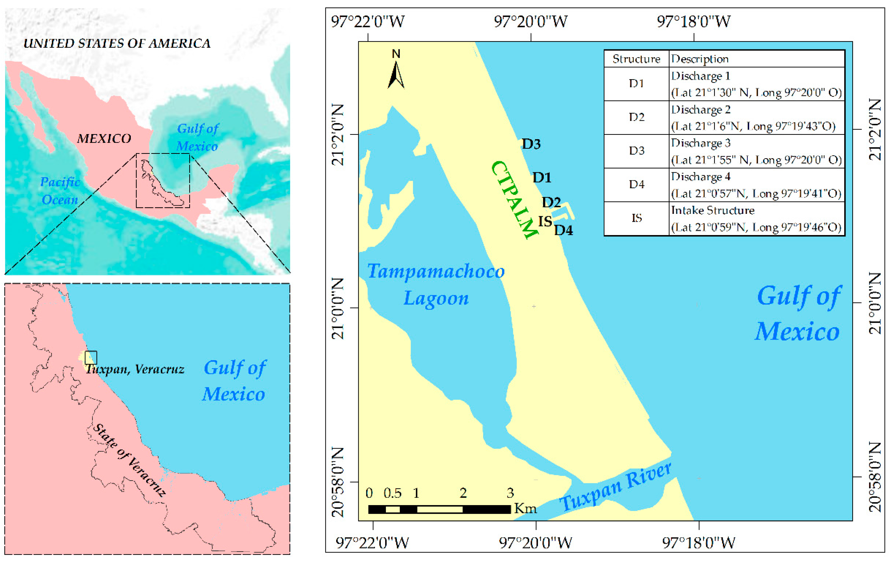
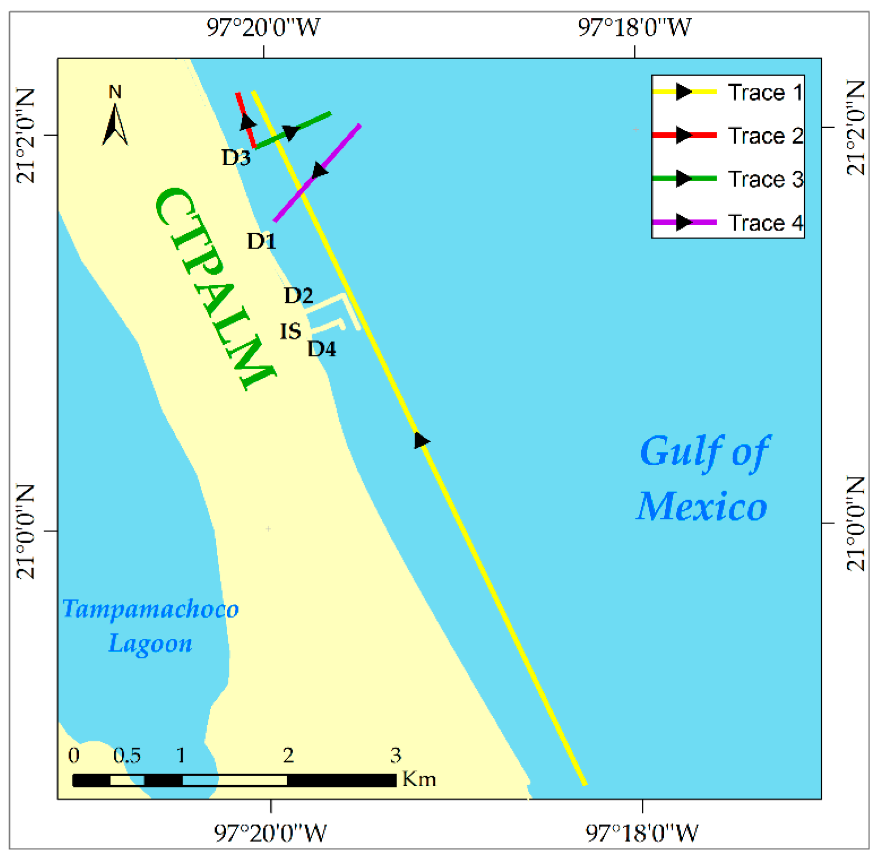
2.1. Case Study

The CTPALM is one of the most important power plants of Mexico, producing 8000 GWh per year approximately [10]. The plant uses about 90 m³/s of seawater of the Gulf of Mexico (GM) for cooling, then the water is returned to the GM with a temperature increase of about 5 °C through four discharge channels. Figure 1 shows the CTPALM, the location of its four discharges (marked as D1, D2, D3, and D4), and the intake structure (IS). The power plant is situated 18 km from Tuxpan City, Veracruz, Mexico, in a region where a river–lagoon–sea system interacts and comprises the discharge of the Tuxpan River, the Tampamachoco Lagoon, and the coast [11].

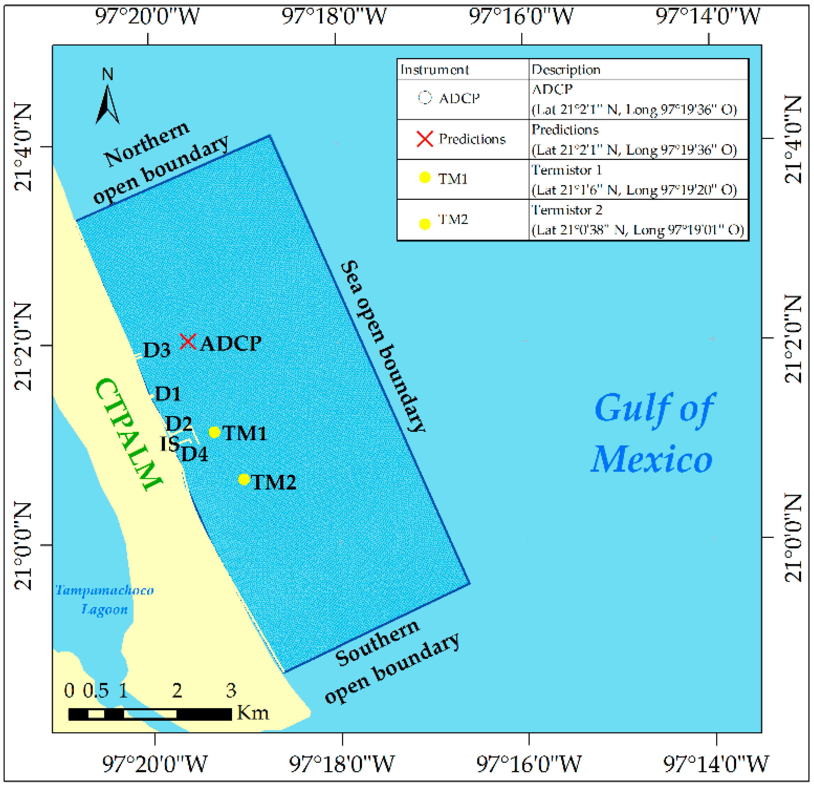
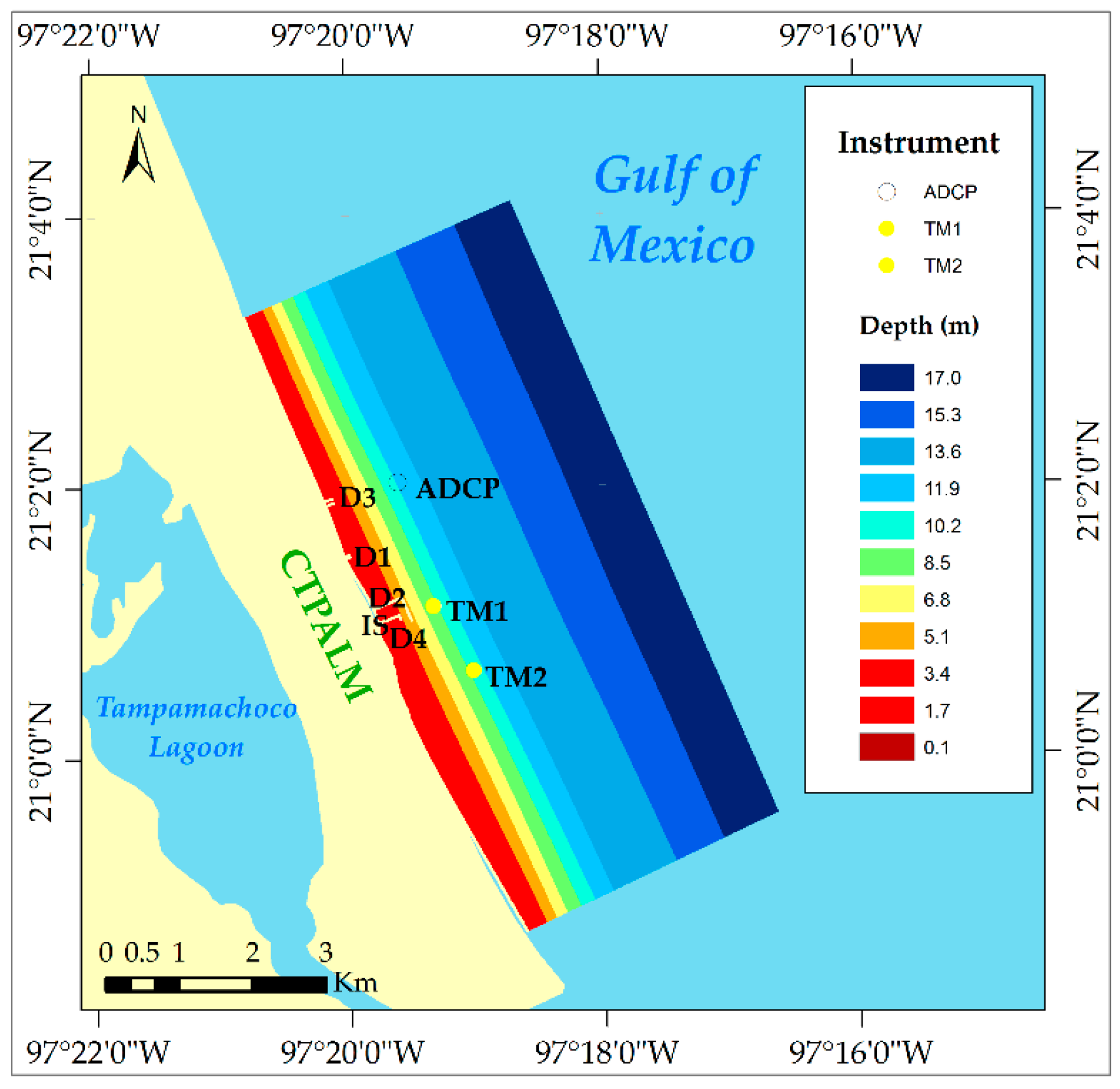
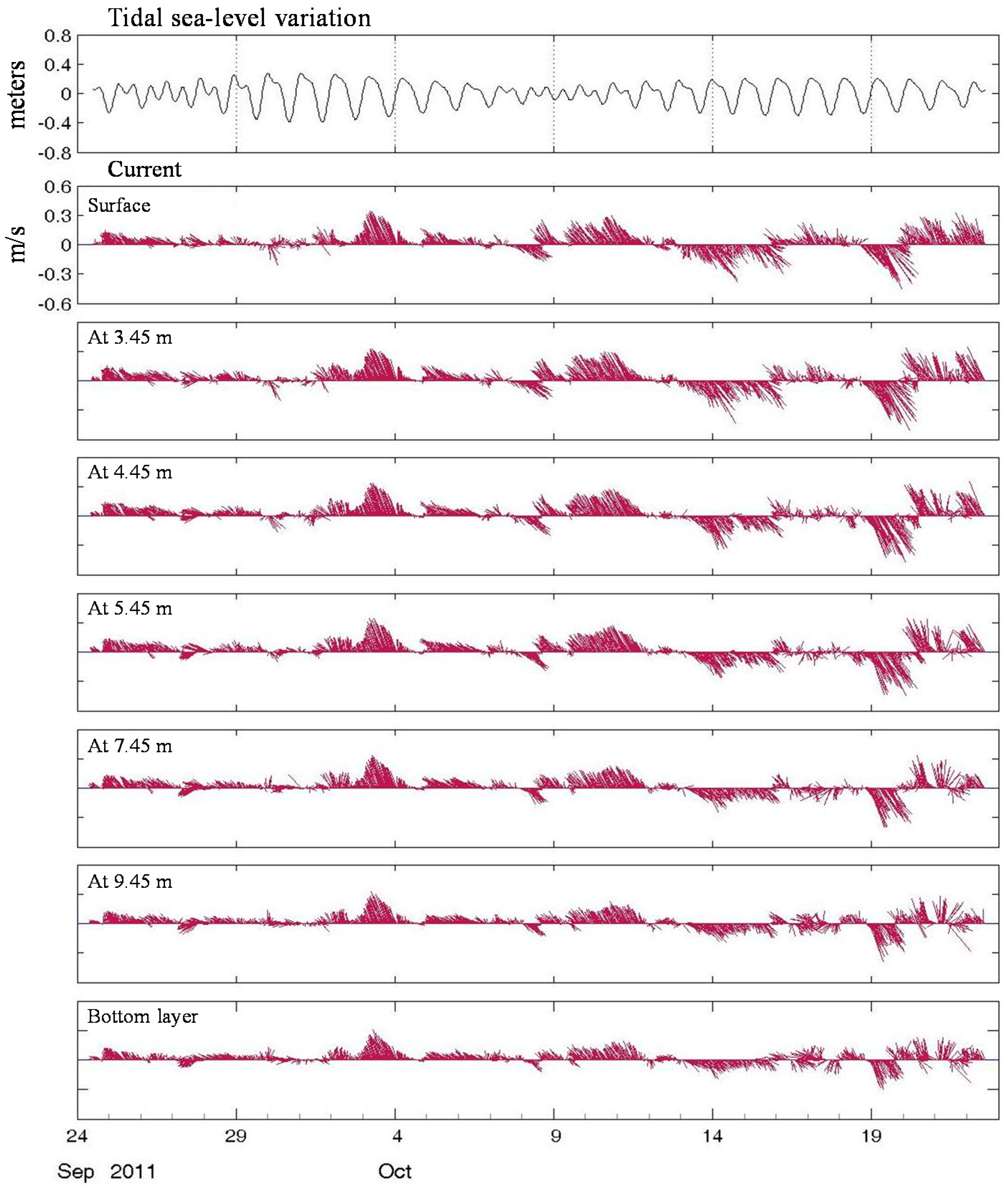
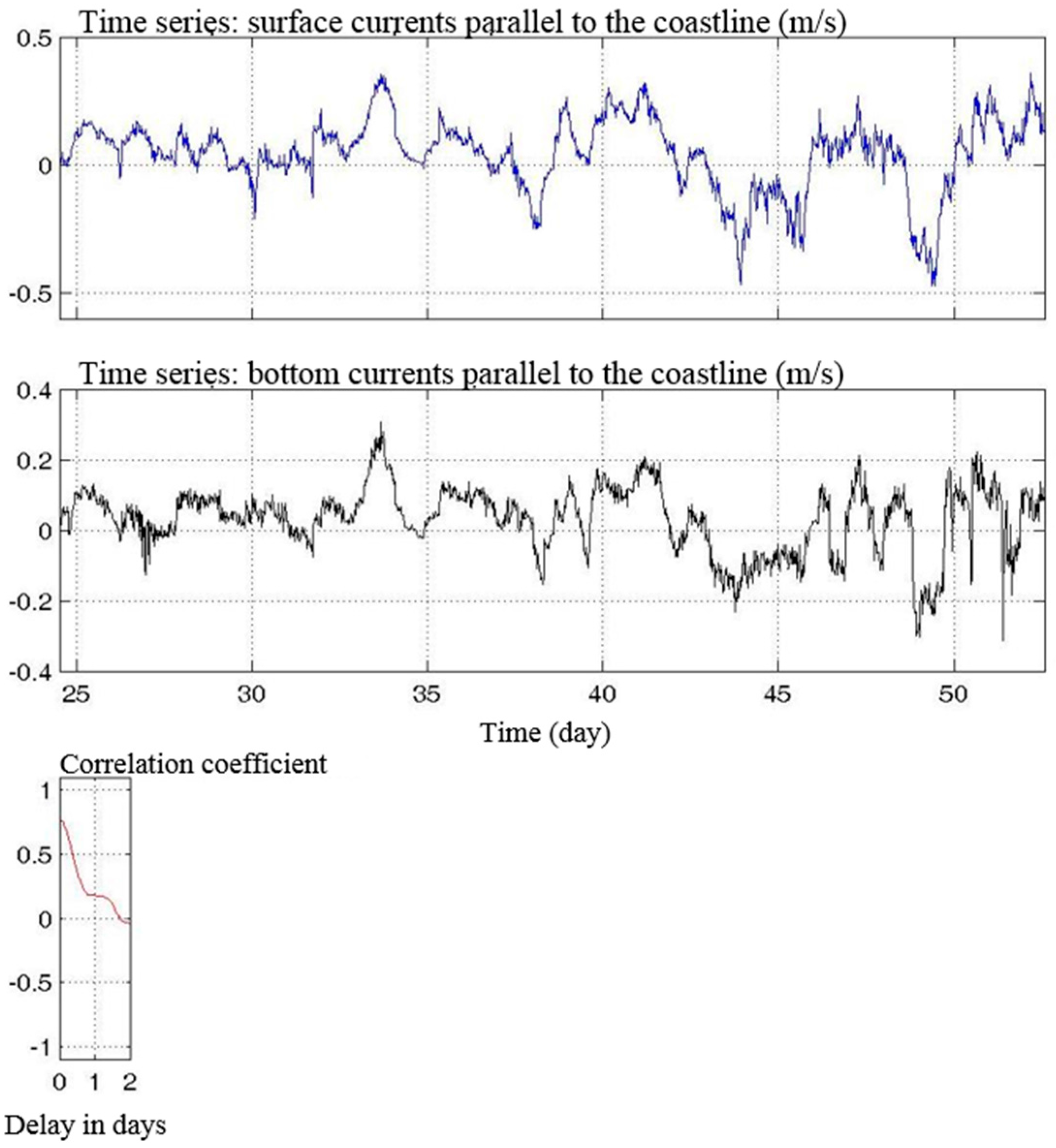
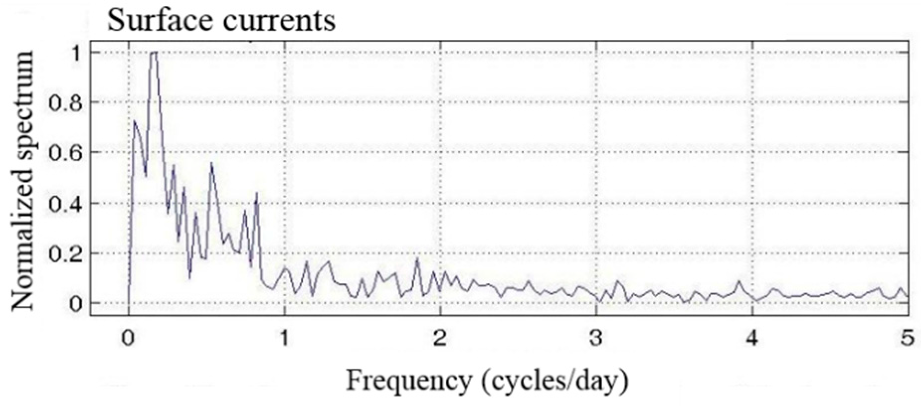
2.2. Field Measurements

Information about the physical parameters prevailing in the study zone was obtained by field investigation and bibliographic compilation. Some information was provided by the CFE and the National Water Commission of Mexico (CONAGUA). The field investigation was conducted in October 2011, when the prevailing weather conditions correspond to a season known as Nortes in Mexico. In these latitudes, the Nortes season coincides with winter, approximately from October to February. This season is characterized by a series of cold fronts that generate strong winds and sudden changes in weather, especially along the coast of the GM. In this region, the force of a cold front is able to drive the mass of water in the direction of its movement, which is generally from northwest to southeast. A decrease in the air temperature and the seawater temperature is also an effect of the passage of a cold front.

The field investigation was planned to provide real-time and long-term measurements. Various instruments were installed inshore just in front of the power plant at many observation points. The parameters measured were currents, tides, seawater temperature, and bathymetry. The data were used to identify the driving forces of the study area and to implement the numerical model.

To measure currents and sea level variations, an Acoustic Doppler Profiler (ADCP) was used. The instrument is a SonTek ADCP, high-performance, 3D water current profiler, with a frequency of 500 kHz, equipped with a pressure sensor. The ADCP was mounted on the seafloor at a depth of 12.15 m, about 1 km seaward, directly in front of Discharge 3 (see Figure 2).

The bathymetry along the coast in front of the power plant was measured using an echo sounder with GPS, for points distributed in a rectangular mesh. The depth measured by the sounder was corrected for the astronomical tidal conditions. Figure 3 shows the bathymetry of the study zone, which is characterized by contour lines parallel to the shoreline, with a relatively smooth gradient perpendicular to the shore.

Time series of seawater temperature were measured at two different points located in front of the power plant. A mooring with two thermistors was installed at each point, one thermistor at 3 m depth (surface) and the other at 7 m depth (bottom), approximately. The location of each mooring is shown in Figure 2. To observe the influence of the four thermal discharges of the CTPALM in the sea at the sea surface, four thermal traces were performed using boat-based CTD on 14 October 2011, during the passage of a cold front. The first trace was oriented parallel to the shoreline from the Tuxpan River discharge to a point near Discharge 3; the second trace was also oriented parallel to the shoreline starting at a point near Discharge 3 and extending approximately 750 m northward; the third trace was oriented perpendicular to the shoreline starting at a point near Discharge 3 and extending seaward approximately 700 m; and the fourth trace was also oriented perpendicular to the shoreline starting further out in the sea and returning coastward to a point near Discharge 1 (see Figure 4). These measurements were taken up to 0.1 m depth at most, in the course of the traces.

2.3. Numerical Model

The numerical model used here is the Delft3D-FLOW model. This model was developed by Deltares Institute of Netherlands and has been applied around the world for many studies. The numerical model simulates unsteady flow in water bodies and can be applied in a two-dimensional or three-dimensional mode, depending on the vertical structure of the flow under study. The system of equations consists of the horizontal equations of motion, the continuity equation, and the transport equations for conservative constituents. In the horizontal direction, Delft3D-FLOW uses orthogonal curvilinear co-ordinates whereas in the vertical direction uses a σ or a Z co-ordinate system. In combination with an appropriate set of initial and boundary conditions, the system of equations is solved on a finite difference staggered grid. Specific details about the time integration method, the particular spatial discretization of the advection terms, turbulence modeling, and more model scopes can be consulted in [12,13,14,15,16,17,18,19,20], respectively. Moreover, some recent similar works to the present one can be consulted in [21,22,23].

2.4. Implementation of the Numerical Model

The computational domain implemented for the numerical simulations is shown in Figure 2. The surface covers a coastal front of 9 km and extends 3.7 km seaward. The intake structure of the CTPALM, together with its four discharges, is located on the coastal line boundary. The northern, southern, and eastern boundaries are considered sea open boundaries. The discrete domain consists of a two-dimensional curvilinear grid of $290\times 128$ cell elements (see Figure 2). The use of a two-dimensional grid is justified by a barotropic vertical flow structure, observed in the study zone with the aid of the ADCP measurements (see Section 3.1). The elements are quasi-rectangular with an approximate size of 30 m in each horizontal dimension. A maximum aspect ratio of 1.5 is obtained in some regions near the coastal line.

For the numerical simulations the sea level variation measured with the ADCP is imposed at the eastern open boundary and free flow is considered at the northern and southern open boundaries. The initial velocities are set to zero and the temperature is imposed uniform according with the data of the thermistors. This same initial temperature is also imposed at the sea open boundaries. The constant flow rates and constant temperatures considered in the simulation for both the intake structure and the four discharges were provided by the CFE. The physical parameters used for the numerical simulations are shown in

Table 1. Initial conditions and physical parameters used for the numerical simulations.

Parameter	Value	Time Variation
Initial velocities	0 m/s
Initial temperature	29.2 from thermistors
Temperature at open boundaries	29.2 from thermistors	Fluctuation, according to the thermistors’ signal
Discharge 1	50.058 m3/s	Constant
Temperature of Discharge 1	34.89 °C	Constant
Discharge 2	4.432 m3/s	Constant
Temperature of Discharge 2	33.58 °C	Constant
Discharge 3	30.087 m3/s	Constant
Temperature of Discharge 3	34.55 °C	Constant
Discharge 4	1.43 m3/s	Constant
Temperature of Discharge 4	32.57 °C	Constant
Suction flow rate at intake	90 m3/s	Constant

.

Winds are assumed to be uniformly distributed over the study area and vary in accordance with data reported for the study period by the weather station 766400 (owned by CONAGUA), located in Tuxpan City at Lat. 20.95° N and Long. 97.4° W. Other climatological parameters such as air temperature and relative humidity were also obtained from the weather station and are used in the Delft3F-FLOW heat flux model.

The time period for the numerical simulations was defined with the aid of the ADCP velocity measurements and existing climatological data. The simulation time period began on 13 October and ended on 15 October 2011. During this period, the cold front Number 6 of the 2011 Nortes season was reported by the CFE. This meteorological phenomenon affected the nearshore current direction, which completely changed from northwest to southeast during the occurrence of this event, as discussed in Section 3.1. This scenario was selected for this study because it is an extraordinary event characterized by strong winds and occurred within a relatively short time window, causing sudden weather changes. The discrete time step is set to 12 s for all the numerical simulations.

3. Results and Discussion

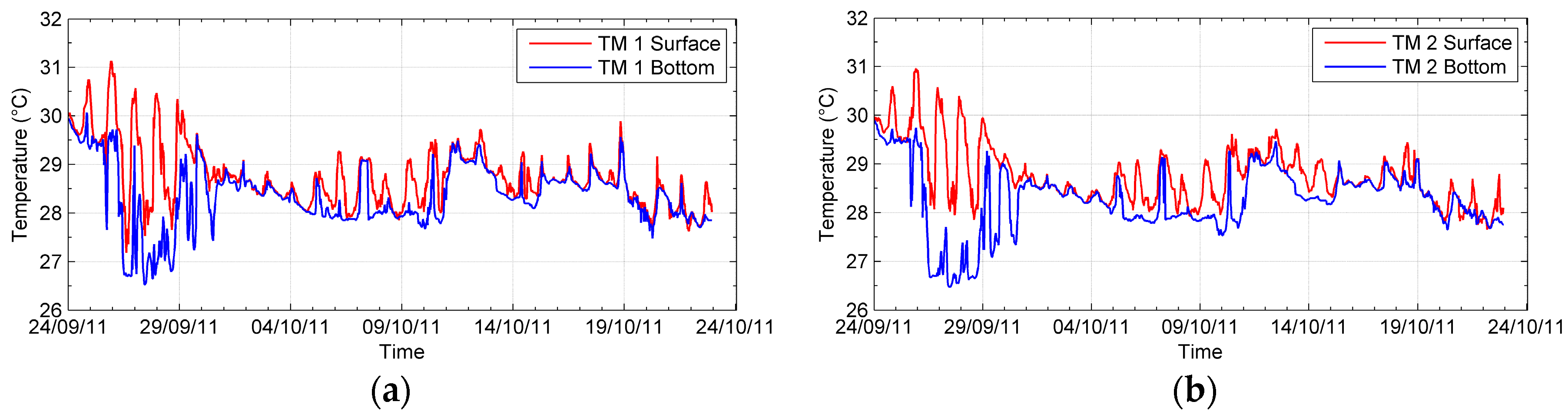
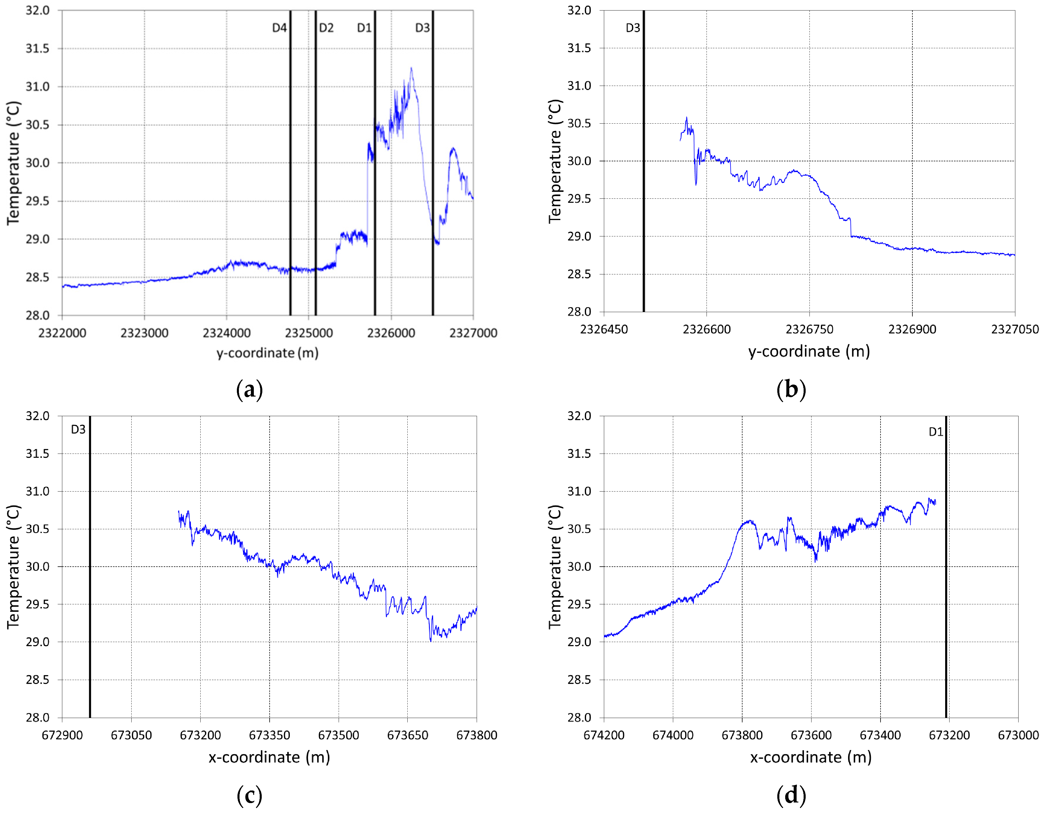
3.1. Results of the Field Measurements

The ADCP measurements of the flow velocity time series at different layers and sea level variations are shown in Figure 5. Data of the ADCP reveal two significant features: the similarity of the currents through the water column, and the directionality of flow. Regarding the similarity, vertical homogeneity is evident and can be attributed to both the shallow depth of the zone and the absence or low impact of water mass flow with different physical or chemical properties. Regarding the directionality, two naturally preferred directions were observed, northwest and southeast, presumably attributable to the shoreline alignment. After a correlation analysis between the velocity of the upper layer and the velocity of the lower layer, a barotropic structure can be deduced (see Figure 6). Regarding the variability of cycle rates of the currents, a signal analysis shows that the velocity series are dominated by low frequencies, much lower than the frequency of the astronomical tide, where the higher one is around 0.016 cycles/day of a period of 25.6 days (see Figure 7). Accordingly, during the period of measurements the evolution of the currents is not dependent on tides; it must be attributable to processes having lower frequencies such as regional mass density flow or the recurrence of cold fronts.

In Figure 8, the time series of temperature measured with thermistors are shown. The time series show some deviation between the surface and the bottom temperatures the first days of measurements, which can be attributed to the cold fronts. However, the temperature measurements confirm that the flow structure is adequately mixed, because there are no significant differences between the surface and the bottom temperatures. A gradual decrease of the seawater temperature, characteristic of the transition between autumn and winter, was observed in the time series data.

The sea surface temperature measured with CTD along each of the four traces of Figure 4 is shown in Figure 9. In each of the four traces, a temperature increase can be observed as the boat approaches the point of discharge. The first trace shows a minimum temperature of about 28.4 °C and a peak of 31.3 °C, which yields a maximum observed temperature increase of 2.9 °C (see Figure 9a). The peak observed in first trace corresponds to the heat of Discharge 1, which is the most important source of heat of the power plant. The second peak of about 30.2 °C is evidence of the heat emitted by Discharge 3, the second most important source of heat. The other traces show lower temperature increases of about 1.8 °C (see Figure 9b–d), reaching temperatures up to 30.9 °C. These last three traces hardly shown the heat emitted by Discharges 1 and 3. The traces perpendicular to the shoreline have a quasi-linear temperature decay seaward for the first 1000 m (see Figure 9c,d). Based on the temperature decay lengths observed along the traces with CDT, an influence area of the thermal plumes can be approximated. By considering a reference seawater temperature of 28.66 °C, which is the average of the temperature measured with thermistors TM 1 and TM 2 during the simulation time period, the first and second traces show a decay length of about 2840 m, parallel to the shoreline, while the third and fourth traces show a decay length of about 1000 m, perpendicular to the shoreline. This yields a rectangular surface of 2.84 km², which is assumed to be the approximate sea surface area of the thermal plumes.

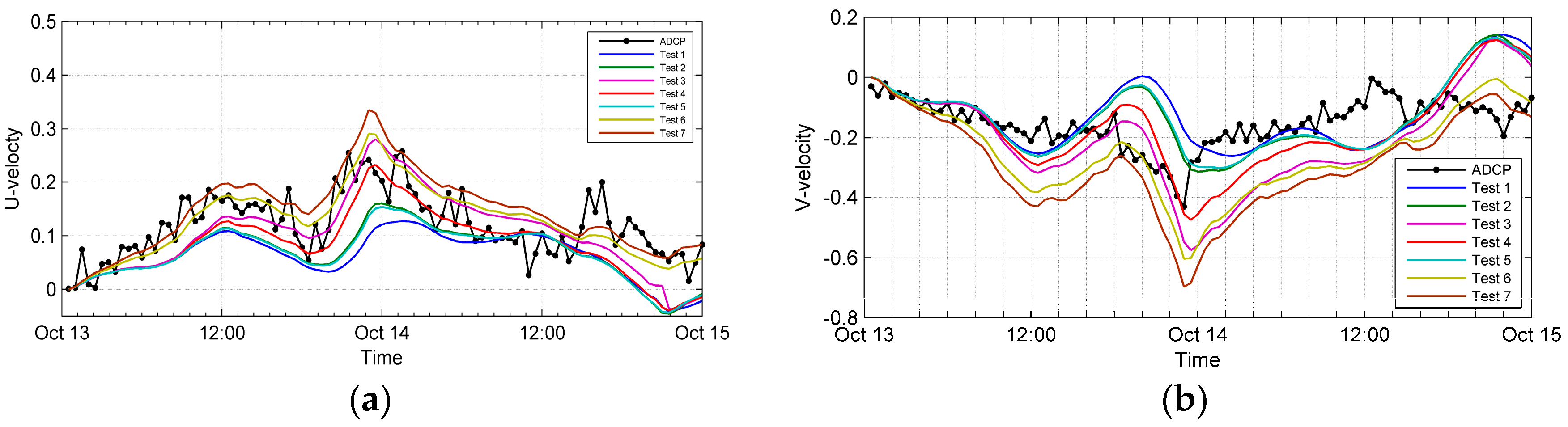
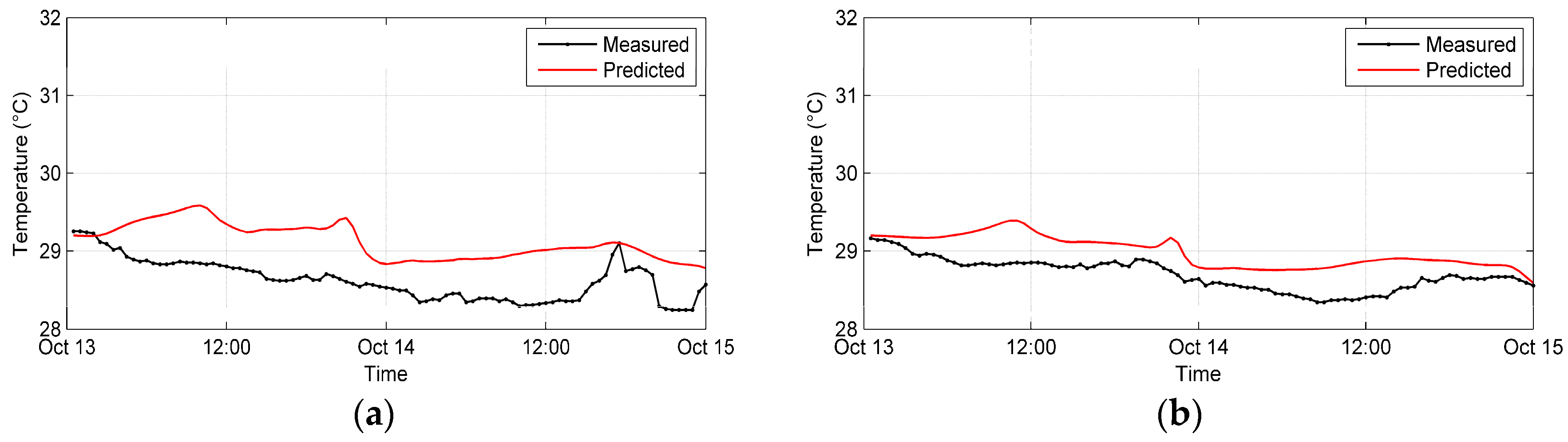
3.2. Calibration and Validation of the Numerical Simulations

Numerical simulations were performed to calibrate and validate the numerical model. The calibration of the dynamic field consisted of a trial wind drag coefficient $C_d$ and Manning coefficient $n$, adjusted in subsequent simulations until the pattern of the predicted depth-averaged horizontal velocities best matched that measured with ADCP over the simulation time period. There is not a specific strategy to define the values of $C_d$; it is a trial and error process in which each result was compared against measurements and then validated. The Manning coefficient has been prescribed according to the literature for different boundary types. Both coefficients were considered to be uniform over the study area and the wind drag coefficient was imposed as a function of wind speed. The parameters used in the calibration tests are presented in

Table 2. Wind drag and Manning coefficients tested during calibration.

Test	Cd	Wind Speed Limits (in m/s)	n
1	0.010 0.007 0.015	<2.5 >2.5, <5.0 >5	0.025
2	0.010 0.030	<2.5 >5.0	0.025
3	0.010 0.020 0.030	>2.5 >2.5, <5.0 >5	0.020
4	0.010 0.020 0.030	<2.5 >2.5, <5.0 >5	0.025
5	0.010	>0	0.025
6	0.030	>0	0.025
7	0.040 0.010	<2.0 >2.0 >5	0.025

.

The predictions of the velocity components were stored at the discrete point shown in Figure 2, which corresponds to the location of the ADCP. In Figure 10, the evolution of measured horizontal velocities and the corresponding predictions are graphed. For the case of $V$-velocity, some tests over-predict or under-predict the peak, whereas others yield matching velocities at the end of the period. For the case of $U$-velocity, most of the tests accurately predicted the pattern, though the velocity is under-predicted in some tests.

The validation of the dynamic field was effectuated over the depth-averaged velocity vector $V=\sqrt{U^2+V^2}$ using the following efficiency criteria:

$$RMSE=\sqrt{\frac{{\displaystyle \sum _{i=1}^k{\left(V_M-V_P\right)}^2}}{k}}$$

(1)

$$m=\frac{{\displaystyle \sum _{i=1}^k\left|V_M-V_P\right|}}{{\displaystyle \sum _{i=1}^k{V}_M}}$$

(2)

where $RMSE$ is the root-mean-square error, $m$ is the mass balance error, the indexes $M$ and $P$ denote measured and predicted values, respectively, and $k$ is the total number of data points. The different coefficients obtained in each calibration test are shown in

Table 3. Calculated coefficients for each calibration test.

Coeff	Calibration Test							Range	Perfect Match
	1	2	3	4	5	6	7
RMSE	0.110	0.096	0.120	0.087	0.099	0.132	0.168	(0,∞)	0
m	0.380	0.360	0.480	0.360	0.360	0.550	0.710	(0,1)	0

, where the range of possible values and the perfect match value are specified for both criteria in the two last columns.

According to the efficiency criteria, some predictions are poorly consistent with measurements. However, despite the complexity of the case study where diverse parameters interact, the flow directionality is well predicted in all calibration tests, as Figure 10 shows. Based on both efficiency criteria, test 4 better approximates the measurements, with RMSE = 0.087 and m = 0.360. Thus, the wind drag coefficients $C_d$ and the Manning coefficient $n$ of test 4 were retained for simulations (see Table 2).

Both efficiency criteria, the root-mean-square error and the mass balance error, were also applied to compare the temperature measured with the thermistors and the depth-averaged predicted temperature. The time series between the surface and the bottom temperatures measured at each point TM 1 and TM 2 (see Figure 8) were averaged to be able to compare with the depth-averaged predicted temperature. Figure 11 shows the evolution of depth-averaged measured and predicted temperatures and

Table 4. Calculated efficiency coefficients for each thermistor.

Coeff	Thermistor		Range	Perfect Match
	TM 1	TM 2
RMSE	0.28	0.10	(0,∞)	0
m	0.02	0.01	(0,1)	0

summarizes the calculated coefficients over the simulation time period. Although both efficiency criteria provide good results, the evolution of measured and predicted temperatures shows that the numerical simulation tends to overestimate the temperature in both points TM 1 and TM 2. The point where the highest differences were obtained is TM 1, but these differences do not exceed 1 °C. At point TM 2, these differences are slightly lower. It is difficult to determine whether the predictions of temperature are good or bad given the different sources of uncertainty involved in the study case, such as the precision of the thermistors or the quality of the meteorological data considered as boundary conditions for the heat flux model. Thus, a maximum range of 1 °C in the differences between measured and predicted temperatures may be considered acceptable.

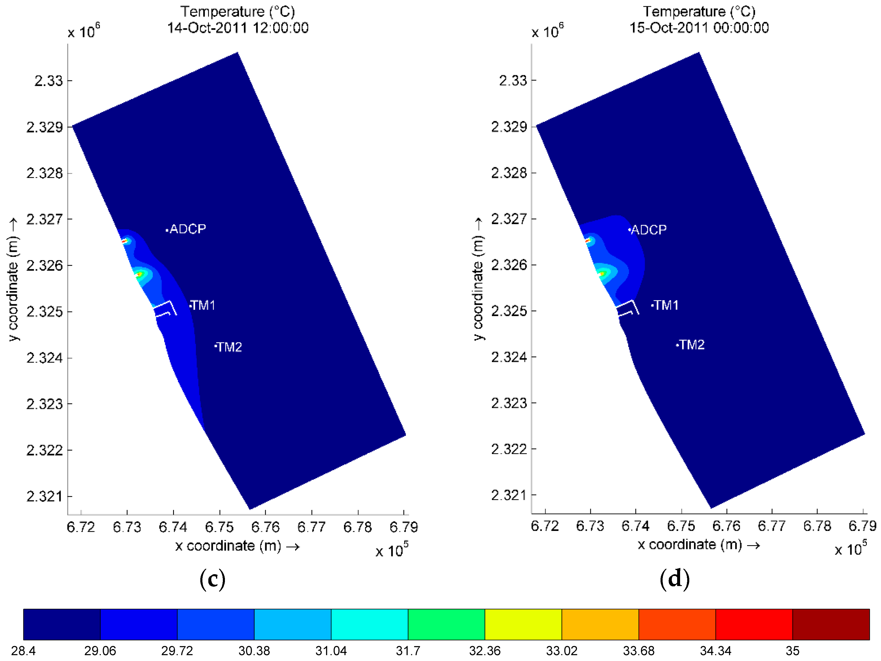
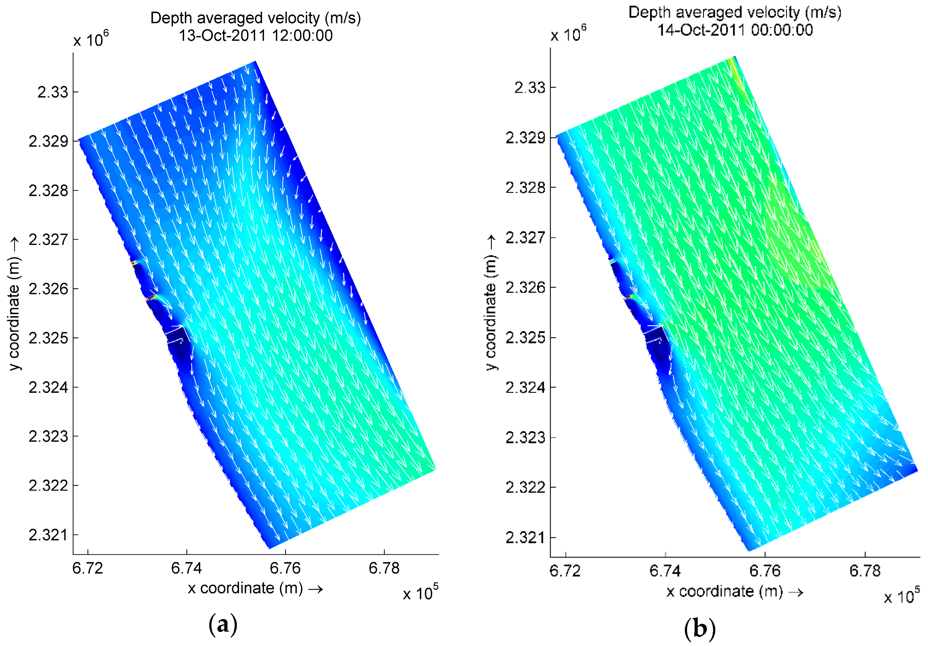
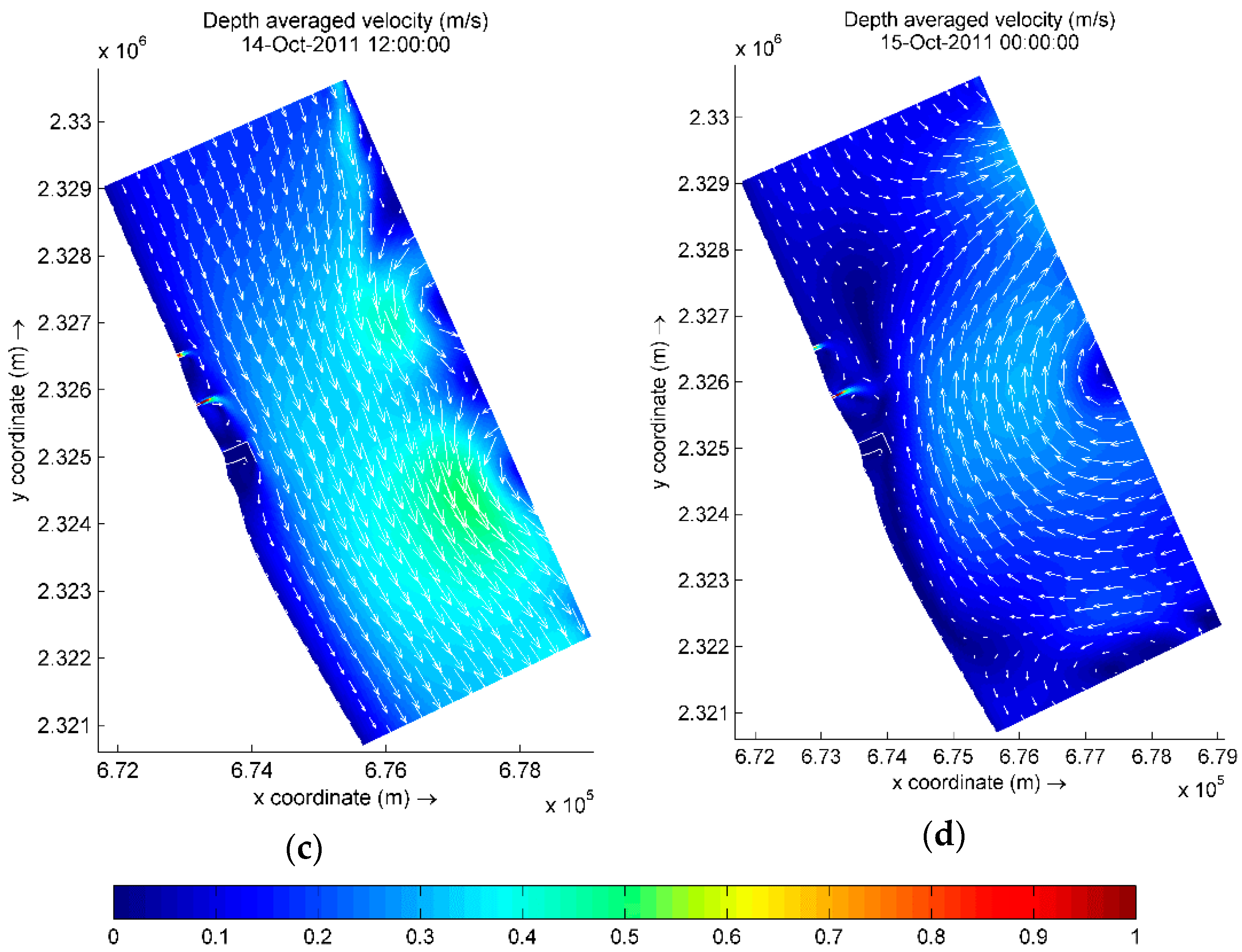
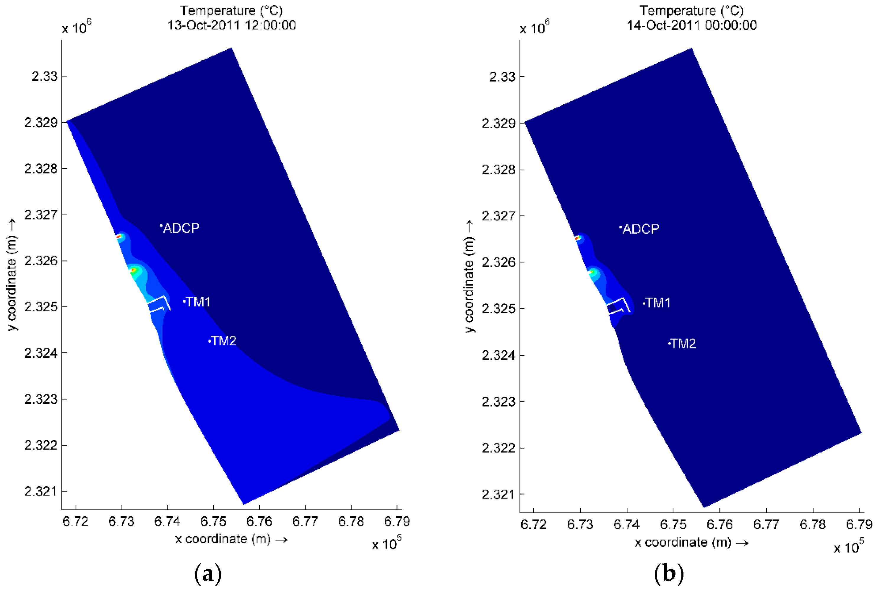
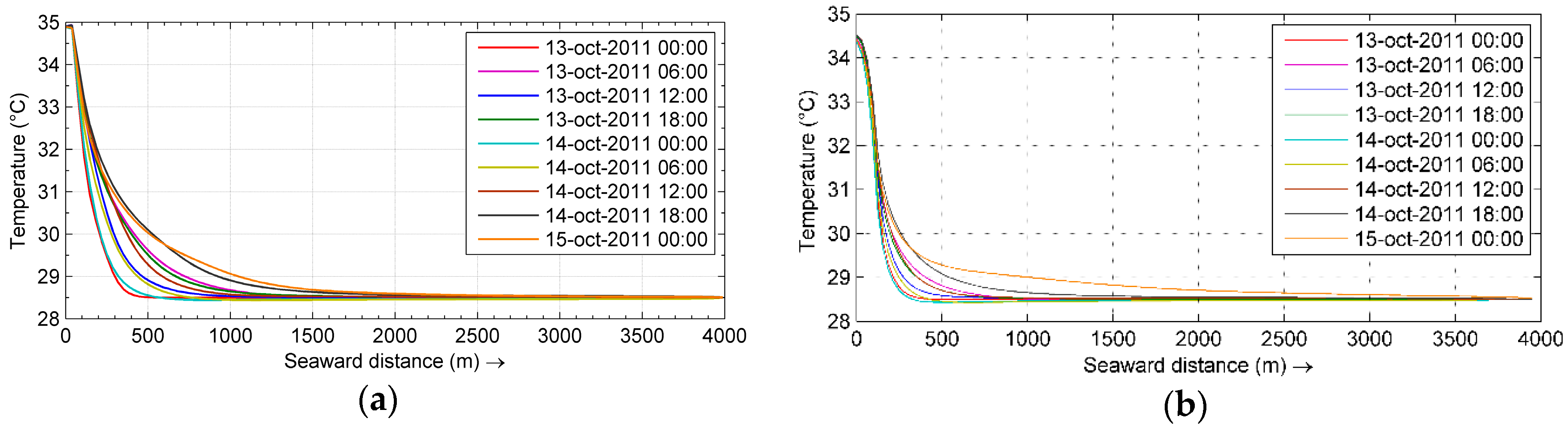
3.3. Thermal Plume Dispersion

Figure 12 shows the current velocity vectors and magnitudes at time intervals of 12 h. As can be observed, the currents maintain a predominantly southward direction, which means that the driven force is the wind acting on the free surface during the passage of the cold front. During the simulation time period, the current velocities reach magnitudes up to 0.4 m/s in the offshore region, whereas the maximum velocities occur near the discharges of the power plant, reaching values greater than 1.0 m/s. In this case, the effects of tides or typical regional mass density flow on the hydrodynamics are not significant. As the winds weaken, these mechanisms have more and more influence on the currents. Other existing studies [9] have shown the significant effects of the tide, which differs from the results observed for the present specific case study.

The thermal plume dispersion is highly influenced by the magnitude and direction of the currents. Figure 13 illustrates the evolution of the predicted thermal field for the same time intervals used in Figure 12. The four thermal discharges of the power plant can be clearly observed with the aid of the isotherms. Because of the predominant flow direction toward the southeast, the thermal plumes are dispersed in the same general direction. Moreover, the plumes are dispersed along the coast, at least during the cold front, for the first 24 h of the simulation time period (see Figure 13a–c). When the cold front weakens at the end of the simulation time period, a seaward thermal dispersion is observed. It is evident that the influence area of the thermal plumes of Discharges 1 and 3 is larger than the area covered by the thermal plumes of Discharges 2 and 4. This is likely because the discharge rate at Discharge 1 and 3 is significantly greater than for Discharge 2 and 4. The directionality developed by the thermal plume dispersion is undesirable from the point of view of the efficiency of the power plant, because large amounts of hot water emitted from Discharges 1 and 3 could recirculate toward the intake. As mentioned above, the efficiency of the power plant is compromised while hot water is taken for cooling.

Table 5. Calculated influence areas of the thermal plumes per range of temperature.

Isotherm (in °C)	Temperature Difference with Respect to 34.89 °C (in °C)	% of Heat Dissipated	Influence Area (in m2)
			13 Oct. at 12:00	14 Oct. at 00:00	14 Oct. at 12:00	15 Oct. at 00:00
34.34	0.55	9	1695	402.8	1710	604.78
33.68	1.21	19	4748	2856	4800	3787
33.02	1.87	30	8635	5371	8733	7291
32.36	2.53	41	15,704	8562	15,390	13,037
31.7	3.19	51	33,607	14,699	31,130	27,652
31.04	3.85	62	74,079	30,605	67,214	69,611
30.38	4.51	72	235,028	66,346	158,387	193,222
29.72	5.17	83	856,495	220,195	534,342	674,638
29.06	5.83	94	12,010,000	823,879	2,420,704	1,843,919

shows the calculated influence areas per range of temperature at time intervals of 12 h. The temperature differences refer to the temperature of Discharge 1, 34.89 °C, which is the highest. The percentages of heat dissipated are calculated considering the maximum temperature difference of 6.23 °C, which corresponds to the difference between the temperature of Discharge 1 and the average of the thermistor measurements of 28.66 °C. The isotherm 29.06 °C covers an area of almost 12 km² during the first 12 h (13 October at 12:00), which is the area of maximum influence of the simulation time period. With this temperature value, the plume has dissipated 94% of heat. After the first 24 h of the simulation time period (14 October at 00:00), the influence area of the isotherm 29.06 °C decreases to reach approximately 0.82 km². This occurs when the current velocities are more intense over the whole study domain, as Figure 12 shows for 14 October at 00:00. After 36 h of the simulation time period (14 October at 12:00), the influence area of the isotherm 29.06 °C covers a surface of approximately 2.42 km². At this particular time, the calculated influence area agrees well with that estimated at the sea surface with the aid of the CTD measurements the same day (see Section 3.1), which is approximately 2.84 km². At all time intervals, the isotherm 29.72 °C, which corresponds to 83% of heat dissipated, significantly decreases the influence area with respect to the area covered by the isotherm 29.06 °C. The influence areas of the rest of the isotherms gradually decrease as the temperature increases to reach low heat dissipation regions, covering relatively small influence areas.

In order to observe the decay length of the thermal plumes for Discharges 1 and 3, the decay curves of temperature along the axis (seaward) were graphed at time intervals of 6 h (see Figure 14). For the case of Discharge 1 (see Figure 14a), 90% of the temperature is dissipated within about 1500 m from the outfall for all time intervals. On the other hand, the temperature of Discharge 3 (see Figure 14b) is dissipated in a shorter distance, 90% within about 750 m. Thus, the plume effects are local, which is confirmed by the CTD measurements of Figure 8.

The temperature history was recorded at the intake, just between the two breakwaters of the plant, to observe thermal recirculation to the power plant (see Figure 15). Compared against 28.66 °C, the average of the thermistor measurements during the simulation time period, the maximum temperature increase observed during the simulation time period is about 1.1 °C. This increase is about 17.66% of 6.23 °C, the maximum temperature difference defined above; thus, it can be considered as not significant. Given the directionality shown by the thermal plumes dispersion, the position of the breakwater north of the plant protects the intake from recirculating thermal flow coming from Discharges 1, 2, and 3. Thus, the plume dispersion that occurred during the cold front passage did not significantly affect the efficiency of the cooling systems of the power plant, regarding thermal plume recirculating.

4. Conclusions

The thermal plume dispersion from the CTPALM discharges has been successfully characterized by numerical modeling. In order to analyze the relevant features of the study zone and to implement the numerical model, a field investigation was also performed. The scenario of a cold front, particularly studied here, revealed that the strong winds occurring during the passage of this phenomenon are capable of causing significant changes in the local coastal hydrodynamics and in thermal plume dispersion as a consequence. Under this scenario, northward winds along the coast result in thermal plume dispersion southward parallel to the shoreline where the power plant intake is located; however, the north breakwater protects it from recirculating hot water. The main hot water source of the power plant comes from Discharges 1 and 3, with a contribution of 93% of the total discharge. Results also showed that the influence area of the thermal plume is at most 12 km², dissipating almost 94% of heat within the first 1500 m seaward.

Finally, in order to implement an effective monitoring program of the thermal plume and to establish appropriate prevention and mitigation measures in terms of the environmental effects, this study has to be reproduced under different physical conditions to identify the features of other typical seasonal events. Data compilation and additional field measurements are necessary to complement numerical simulations and gather more reliable results.

References

1. Botello, A.V.; Rendón, J. Evaluación del Impacto ambiental de la central Nucleoeléctrica Laguna Verde a 15 años de operación. In Golfo de México. Contaminación e Impacto Ambiental: Diagnóstico y Tendencias, 2nd ed.; Botello, A.V., Rendón, J., Bouchot, G.G., Hernández, C.A., Eds.; EPOMEX: Campeche, Mexcio, 2005. [Google Scholar]
2. Silva, H.A.; Botello, A.V. Evaluación del Impacto ambiental de la central Nucleoeléctrica Laguna Verde. In Golfo de México. Contaminación e Impacto Ambiental: Diagnóstico y Tendencias; EPOMEX: Campeche, Mexcio, 1996. [Google Scholar]
3. Maupin, M.A.; Kenny, J.F.; Hutson, S.S.; Lovelace, J.K.; Barber, N.L.; Linsey, K.S. Estimated Use of Water in the United States in 2010; Circular 1405; U.S. Geological Survey: Reston, VA, USA, 2014; p. 56.
4. Ramírez-León, H.; Couder-Castaneda, C.; Herrera-Díaz, I.E.; Barrios-Pina, H.A. Modelación numérica de la descarga térmica de la Central Nucleoeléctrica Laguna Verde. Revista Internacional Métodos Numéricos Cálculo Diseño Ingeniería 2013, 29, 114–121. [Google Scholar] [CrossRef]
5. Huang, X.; Zhu, Z.; Xu, M.; Jing, Q. Variation of Water Temperature in the Southwestern Daya Bay before and after the Operation of Daya Bay Nuclear Power Plant; Annual Research Reports; Marine Biology Research Station at Daya Bay: Beijing, China, 1998; pp. 102–112. [Google Scholar]
6. Donlon, C.J.; Minnett, P.J.; Gentemann, C.; Nightingale, T.; Barton, I.J.; Ward, B.; Murray, M.J. Toward improved validation of satellite sea surface skin temperature measurements for climate research. J. Clim. 2002, 15, 353–369. [Google Scholar] [CrossRef]
7. Ahn, Y.-H.; Shanmugam, P.; Lee, J.-H.; Kang, Y.Q. Application of satellite infrared data for mapping of thermal plume contamination in coastal ecosystem of Korea. Mar. Environ. Res. 2006, 61, 186–201. [Google Scholar] [CrossRef] [PubMed]
8. Buvaneshwari, S.; Ravichandran, V.; Mudgal, B.V. Thermal pollution of cooling water discharge into a closed creek system. Indian J. Mar. Sci. 2014, 43, 1–7. [Google Scholar]
9. Salgueiro, D.V.; de Pablo, H.; Neves, R.; Mateus, M. Modelling the thermal effluent of a near coast power plant (Sines, Portugal). J. Integr. Coast. Zone Manag. 2015, 15, 533–544. [Google Scholar] [CrossRef]
10. Secretaría de Energía. 2014 Balance Nacional de Energía; Subsecretaría de Planeación y Transición Energética, Dirección General de Planeación e Información Energéticas: Ciudad de México, Mexico, 2013. [Google Scholar]
11. Barrios-Piña, H.A.; Ramírez-León, H.; Rodríguez-Cuevas, C.; Torres-Bejarano, F. Estudio Hidrodinámico y de dispersión de plumas térmicas en zonas costeras. In Proceedings of the XXV Congreso Latinoamericano de Hidraúlica, Santiago, Chile, 25–29 August 2014.
12. Leendertse, J.J.; Alexander, R.C.; Liu, S.K. A Three-Dimensional Model for Estuaries and Coastal Seas: Volume I, Principles of Computations; Report R-1417-OWRR; Rand Corporation: Santa Monica, CA, USA, 1973. [Google Scholar]
13. Leendertse, J.J.; Liu, S.K. A Three-Dimensional Model for Estuaries and Coastal Seas: Volume II: Aspects of Computation; Report R-1764-OWRT; Rand Corporation: Santa Monica, CA, USA, 1975. [Google Scholar]
14. Leendertse, J.J.; Liu, S.K.; Nelson, A.B. A Three-Dimensional Model for Estuaries and Coastal Seas: Volume III, The Interim Program; Report R-1884-OWRT; Rand Corporation: Santa Monica, CA, USA, 1975. [Google Scholar]
15. Leendertse, J.J.; Liu, S.K. A Three-Dimensional Model for Estuaries and Coastal Seas: Volume IV, Turbulent energy computation; Report R-2187-OWRT; Rand Corporation: Santa Monica, CA, USA, 1977. [Google Scholar]
16. Stelling, G.S. On the Construction of Computational Methods for Shallow Water Flow Problems. Ph.D. Thesis, Delft University of Technology, Delft, The Netherlands, December 1983; p. 35. [Google Scholar]
17. Stelling, G.S.; Leendertse, J.J. Approximation of Convective Processes by Cyclic AOI methods. In Proceeding of the 2nd Conference on Estuarine and Coastal Modeling, Tampa, FL, USA, 13–15 November 1991; Spaulding, M.L., Bedford, K., Blumberg, A., Eds.; American Society of Civil Engineers: New York, NY, USA, 1992; pp. 771–782. [Google Scholar]
18. Stelling, G.S.; Duinmeijer, S.P.A. A staggered conservative scheme for every Froude number in rapidly varied shallow water flows. Int. J. Numer. Methods Fluids 2003, 43, 1329–1354. [Google Scholar] [CrossRef]
19. Uittenbogaard, R.E.; van Vossen, B. Subgrid-scale model for Quasi-2D turbulence in shallow water. In Shallow Flows; Uijttewaal, W.S.J., Jirka, G.H., Eds.; Taylor & Francis: London, UK, 2004; pp. 575–582. [Google Scholar]
20. Deltares. Delft3D-Flow User Manual, 3.15 ed.; Deltares: Delft, The Netherlands, 2011. [Google Scholar]
21. Morelissen, R.; van der Kaaij, T.; Bleninger, T. Dynamic coupling of near field and far field models for simulating effluent discharges. Water Sci. Technol. 2013, 67, 2210–2220. [Google Scholar] [CrossRef] [PubMed]
22. De Graaff, R.; Lindfors, A.; de Goede, E.; Rasmus, K.; Morelissen, R. Modelling of a Thermal Discharge in an Ice-covered Estuary in Finland. In Proceedings of the OTC Arctic Technology Conference, Copenhagen, Denmark, 23–25 March 2015.
23. Duy Vinh, V.; Ouillon, S.; Van Thao, N.; Ngoc Tien, N. Numerical Simulations of Suspended Sediment Dynamics Due to Seasonal Forcing in the Mekong Coastal Area. Water 2016, 8, 255. [Google Scholar] [CrossRef]
Figure 1. Location of the CTPALM power plant.
Water 08 00482 g001
Figure 2. Study domain and location of the ADCP and thermistor moorings.
Water 08 00482 g002
Figure 3. Bathymetry of the study zone.
Water 08 00482 g003
Figure 4. Location of the four traces performed using boat-based CTD on 14 October 2011.
Water 08 00482 g004
Figure 5. Tidal variation and current velocity measured with ADCP.
Water 08 00482 g005
Figure 6. Correlation analysis between the surface and bottom currents, which shows a match, characteristic of a barotropic structure.
Water 08 00482 g006
Figure 7. Frequency spectrum of the surface current parallel to the coastline.
Water 08 00482 g007
Figure 8. Time series of seawater temperature measured in front of the CTPALM. (a) Mooring TM 1; (b) Mooring TM 2.
Water 08 00482 g008
Figure 9. Sea surface CTD temperature measurements in front of the CTPALM. Solid lines show the location of the discharges. (a) First trace; (b) Second trace; (c) Third trace; (d) Fourth trace.
Water 08 00482 g009
Figure 10. Measured and predicted depth-averaged horizontal velocities of the calibration tests. (a) U -velocity; (b) V -velocity.
Water 08 00482 g010
Figure 11. Thermistor measurements and predicted temperature. (a) Depth-averaged temperature at mooring TM 1; (b) Depth-averaged temperature at mooring TM 2.
Water 08 00482 g011
Figure 12. Depth-averaged velocity field (in m/s) at time intervals of 12 h. (a) 13 October 2011 12:00:00; (b) 14 October 2011 00:00:00; (c) 14 October 2011 12:00:00; (d) 15 October 2011 00:00:00.
Water 08 00482 g012aWater 08 00482 g012b
Figure 13. Temperature field (in °C) at time intervals of 12 h. (a) 13 October 2011 12:00:00; (b) 14 October 2011 00:00:00; (c) 14 October 2011 12:00:00; (d) 15 October 2011 00:00:00.
Water 08 00482 g013aWater 08 00482 g013b
Figure 14. Decay curves of temperature following the discharge axes. (a) Discharge 1; (b) Discharge 3.
Water 08 00482 g014
Figure 15. Temperature signal at the intake of the CTPALM.
Water 08 00482 g015