
Mid-Infrared Spectroscopy as a Potential Tool for Reconstructing Lake Salinity


Abstract
:1. Introduction
2. Materials and Methods
3. Results
4. Discussion
5. Conclusions
Acknowledgments
Author Contributions
Conflicts of Interest
References
- Australian Bureau of Statistics (ABS). Measures of Australia’s Progress, 2010; ABS: Canberra, Australia, 2010; p. 223.
- National Land and Water Resources Audit (NLWRA). Australian Dryland Salinity Assessment 2000; NLWRA: Canberra, Australia, 2001; p. 129.
- Gell, P.; Fritz, S.; Battarbee, R.; Tibby, J. LIMPACS-Human and Climate Interactions with Lake Ecosystems: Setting research priorities in the study of the impact of salinisation and climate change on lakes, 2005–2010. Hydrobiologia 2007, 591, 99–101. [Google Scholar] [CrossRef]
- Nielsen, D.L.; Brock, M.A.; Rees, G.N.; Baldwin, D.S. Effects of increasing salinity on freshwater ecosystems in Australia. Aust. J. Bot. 2003, 51, 655–665. [Google Scholar] [CrossRef]
- Australian and New Zealand Environment and Conservation Council (ANZECC). Implications of Salinity for Biodiversity Conservation and Management; Task Force for the Standing Committee on Conservation: Canberra, Australia, 2001; p. 59.
- Gell, P. With the benefit of hindsight: The utility of palaeoecology in wetland condition assessment and identification of restoration targets. In Ecology of Industrial Pollution (Ecological Review Series); Batty, L., Hallberg, K., Eds.; Cambridge University Press & the British Ecological Society: Cambridge, UK, 2010; pp. 162–188. [Google Scholar]
- Pearson, S.; Lynch, A.J.J.; Plant, R.; Cork, S.; Taffs, K.; Dodson, J.; Maynard, S.; Gergis, J.; Gell, P.; Thackway, R.; et al. Increasing the understanding and use of natural archives of ecosystem services, resilience and thresholds to improve policy, science and practice. Holocene 2015, 25, 366–378. [Google Scholar] [CrossRef]
- Juggins, S. Quantitative reconstructions in palaeolimnology: New paradigm or sick science? Quat. Sci. Rev. 2013, 64, 20–32. [Google Scholar] [CrossRef]
- Barry, M.J.; Tibby, J.; Tsitsilas, A.; Mason, B.; Kershaw, P.; Heijnis, H. A long term lake salinity record and its relationship to Daphnia populations. Arch. Hydrobiol. 2005, 163, 1–23. [Google Scholar] [CrossRef]
- Gell, P.; Tibby, J.; Little, F.; Baldwin, D.; Hancock, G. The impact of regulation and salinisation on floodplain lakes: The lower River Murray, Australia. Hydrobiologia 2007, 591, 135–146. [Google Scholar] [CrossRef]
- Kemp, J.; Radke, L.C.; Olley, J.; Juggins, S.; De Deckker, P. Holocene lake salinity changes in the Wimmera, southeastern Australia, provide evidence for millennial-scale climate variability. Quat. Res. 2012, 77, 65–76. [Google Scholar] [CrossRef]
- Gouramanis, C.; Wilkins, D.; De Deckker, P. 6000 years of environmental changes recorded in Blue Lake, South Australia, based on ostracod ecology and valve chemistry. Palaeogeogr. Palaeoclim. Palaeoecol. 2010, 297, 223–237. [Google Scholar] [CrossRef]
- Gouramanis, C.; Dodson, J.R.; Wilkins, D.; De Deckker, P.; Chase, B.M. Holocene palaeoclimate and sea level fluctuation recorded from the coastal Barker Swamp, Rottnest Island, south-western Western Australia. Quat. Sci. Rev. 2012, 54, 40–57. [Google Scholar] [CrossRef]
- Haynes, D.; Skinner, R.; Tibby, J.; Cann, J.; Fluin, J. Diatom and foraminifera relationships to water quality in The Coorong, South Australia, and the development of a diatom-based salinity transfer function. J. Paleolimnol. 2011, 46, 543–560. [Google Scholar] [CrossRef]
- Barr, C.; Tibby, J.; Gell, P.; Tyler, J.; Zawadzki, A.; Jacobsen, G.E. Climate variability in south-eastern Australia over the last 1500 years inferred from the high-resolution diatom records of two crater lakes. Quat. Sci. Rev. 2014, 95, 115–131. [Google Scholar] [CrossRef]
- Tibby, J.; Kershaw, A.P.; Builth, H.; Philibert, A.; White, C. Environmental change and variability in south-western Victoria: Changing constraints and opportunities for occupation and land use. In The Social Archaeology of Australian Indigenous Societies; David, B., Barker, B., McNiven, I., Eds.; Aboriginal Studies Press: Canberra, Australia, 2006; pp. 254–269. [Google Scholar]
- Gell, P.A. The development of diatom database for inferring lake salinity, Western Victoria, Australia: Towards a quantitative approach for reconstructing past climates. Aust. J. Bot. 1997, 45, 389–423. [Google Scholar] [CrossRef]
- Fluin, J.; Gell, P.; Haynes, D.; Tibby, J.; Hancock, G. Palaeolimnological evidence for the independent evolution of neighbouring terminal lakes, the Murray Darling Basin, Australia. Hydrobiologia 2007, 591, 117–134. [Google Scholar] [CrossRef]
- Wang, P.; Chappell, J. Foraminifera as Holocene environmental indicators in the South Alligator River, Northern Australia. Quat. Int. 2001, 83–85, 47–62. [Google Scholar] [CrossRef]
- Danielopol, D.L.; Casale, L.M.; Olteanu, R. On the preservation of carapaces of some limnic ostracods: An exercise in actuopalaeontology. Hyrodbiologia 1986, 14, 143–157. [Google Scholar] [CrossRef]
- Rosén, P.; Vogel, H.; Cunningham, L.; Reuss, N.; Conley, D.; Persson, P. Fourier transform infrared spectroscopy, a new method for rapid determination of total organic and inorganic carbon and biogenic silica concentration in lake sediments. J. Palaeolimnol. 2010, 43, 247–259. [Google Scholar] [CrossRef]
- Rosén, P.; Vogel, H.; Cunningham, L.; Hahn, A.; Hausmann, S.; Pienitz, R.; Zolitschka, B.; Wagner, B.; Persson, P. Universally applicable model for the quantitative determination of lake sediment composition using Fourier transform infrared spectroscopy. Environ. Sci. Technol. 2011, 45, 8858–8865. [Google Scholar] [CrossRef] [PubMed]
- Vogel, H.; Rosén, P.; Wagner, B.; Melles, M.; Persson, P. Fourier transform infrared spectroscopy, a new cost-effective tool for quantitative analysis of biogeochemical properties in long sediment records. J. Palaeolimnol. 2008, 40, 689–702. [Google Scholar] [CrossRef]
- Smith, B.C. Fundamentals of Fourier Transform Infrared Spectroscopy, 2nd ed.; CRC Press: Boca Raton, FL, USA, 2011; p. 207. [Google Scholar]
- Farmer, V.C. The Infra-Red Spectra of Minerals; Mineralogical Society: London, UK, 1974; p. 539. [Google Scholar]
- Meyers, P.A.; Ishiwatari, R. Lacustrine organic geochemistry—An overview of indicators of organic-matter sources and diagenesis in lake-sediments. Org. Geochem. 1993, 20, 867–900. [Google Scholar] [CrossRef]
- Masserschmidt, I.; Cuelbas, C.J.; Poppi, R.J.; de Andrade, J.C.; de Abreu, C.A.; Davanzo, C.U. Determination of organic matter in soils by FTIR/diffuse reflectance and multivariate calibration. J. Chemom. 1999, 13, 265–273. [Google Scholar] [CrossRef]
- Viscarra Rossel, R.A.; McGlynn, R.N.; McBratney, A.B. Determining the composition of mineral-organic mixes using UV–vis–NIR diffuse reflectance spectroscopy. Geoderma 2006, 137, 70–82. [Google Scholar] [CrossRef]
- Minasny, B.; Tranter, G.; McBratney, A.B.; Brough, D.M.; Murphy, B.W. Regional transferability of mid-infrared diffuse reflectance spectroscopic prediction for soil chemical properties. Geoderma 2009, 153, 155–162. [Google Scholar] [CrossRef]
- McCarty, G.W.; Reeves, J.B., III; Reeves, V.B.; Follett, R.F.; Kimble, J.M. Mid-infrared and near-infrared diffuse reflectance spectroscopy for soil carbon measurement. Soil Sci. Soc. Am. J. 2002, 66, 640–646. [Google Scholar]
- Janik, L.J.; Skjemstad, J.O. Characterisation and analysis of soils using mid infrared partial least-squares. 2. Correlations with some laboratory data. Aust. J. Soil Res. 1995, 33, 637–650. [Google Scholar] [CrossRef]
- Forrester, S.; Janik, L.; McLaughlin, M.; Soriano Disla, M.; Stewart, R.; Dearman, B. Total Petroleum Hydrocarbon Concentration Prediction in Soils Using Diffuse Reflectance Infrared Spectroscopy. Soil Sci. Soc. Am. J. 2013, 77, 450–460. [Google Scholar] [CrossRef]
- Liu, X.; Colman, S.M.; Brown, E.T.; Minor, E.C.; Li, H. Estimation of carbonate, total organic carbon, and biogenic silica content by FTIR and XRF techniques in lacustrine sediments. J. Paleolimnol. 2013, 50, 387–398. [Google Scholar] [CrossRef]
- Hahn, A.; Rosén, P.; Kliem, P.; Ohlendorf, C.; Persson, P.; Zolitschka, B.; the PASADO Science Team. Comparative study of infrared techniques for fast biogeochemical sediment analyses. Geochem. Geophys. 2011, 12, Q10003. [Google Scholar]
- Veerasingam, S.; Venkatachalapathy, R. Estimation of carbonate concentration and characterization of marine sediments by Fourier transform infrared spectroscopy. Infrared Phys. Technol. 2014, 66, 136–140. [Google Scholar] [CrossRef]
- Ji, J.; Ge, Y.; Balsam, W.; Damuth, J.E.; Chen, J. Rapid identification of dolomite using a Fourier Transform infrared spectrophotometer (FTIR): A fast method for identifying Heinrich events in IODP Site U1308. Mar. Geol. 2008, 258, 60–68. [Google Scholar] [CrossRef]
- Janik, L.J.; Merry, R.H.; Skjemstad, J.O. Can mid infra-red diffuse reflectance analysis replace soil extractions? Anim. Prod. Sci. 1998, 38, 681–696. [Google Scholar] [CrossRef]
- Umali, B.P.; Oliver, D.P.; Ostendorf, B.; Forrester, S.; Chittleborough, D.J.; Hutson, J.L.; Kookana, R.S. Spatial distribution of diuron sorption affinity as affected by soil, terrain and management practices in an intensively managed apple orchard. J. Hazard. Mat. 2012, 217–218, 398–405. [Google Scholar] [CrossRef] [PubMed]
- Siebielec, G.; McCarty, G.W.; Stuczynski, T.I.; Reeves, J.B., III. Near- and mid-infrared diffuse reflectance spectroscopy for measuring soil metal content. J. Environ. Qual. 2004, 33, 2056–2069. [Google Scholar] [CrossRef] [PubMed]
- Bertaux, J.; Frölich, F.; Ildefonse, P. Multicomponent analysis of MIRS spectra: Quantification of amorphous and crystallized mineral phases in synthetic and natural sediments. J. Sediment. Res. 1998, 68, 440–447. [Google Scholar] [CrossRef]
- Meyer-Jacob, C.; Vogel, H.; Boxberg, F.; Rosen, P.; Weber, M.E.; Bindler, R. Independent measurement of biogenic silica in sediments by FTIR spectroscopy and PLS regression. J. Paleolimnol. 2014, 52, 245–255. [Google Scholar] [CrossRef]
- Mecozzi, M.; Pietrantonio, E.; Amici, M.; Romanelli, G. Determination of carbonate in marine solid samples by MIR-ATR spectroscopy. Analyst 2001, 126, 144–146. [Google Scholar] [CrossRef] [PubMed]
- Wirrman, H.; Bertaux, J.; Kossoni, A. Late Holocene palaeoclimatic changes in western central Africa inferred from mineral abundances in dated sediments from Lake Ossa (southwestern Cameroon). Quat. Res. 2001, 56, 275–287. [Google Scholar] [CrossRef]
- Ramasamy, V.; Rajkumar, P.; Ponnusamy, V. Depth wise analysis of recently excavated Vellar river sediments through MIRS and XRD studies. Ind. J. Phys. 2009, 83, 1295–1308. [Google Scholar] [CrossRef]
- Belzile, N.; Joly, H.A.; Li, H. Characterization of humic substances extracted from Canadian lake sediments. Can. J. Chem. 1997, 75, 14–27. [Google Scholar] [CrossRef]
- Calace, N.; Cardellicchio, N.; Petronio, B.M.; Pietrantonio, M.; Pietroletti, M. Sedimentary humic substances in the northern Adriatic sea (Mediterranean sea). Mar. Environ. Res. 2006, 61, 40–58. [Google Scholar] [CrossRef] [PubMed]
- Cunningham, L.; Vogel, H.; Nowaczyk, N.; Wennrich, V.; Juschus, O.; Persson, P.; Rosen, P. Climatic variability during the last interglacial inferred from geochemical proxies in the Lake El’gygytgyn sediment record. Palaeogeogr. Palaeoclim. Palaeoecol. 2013, 386, 408–414. [Google Scholar] [CrossRef]
- Rosén, P. Total organic carbon (TOC) of lake water during the Holocene inferred from lake sediments and near-infrared spectroscopy (NIRS) in eight lakes from northern Sweden. Biogeochemistry 2005, 76, 503–516. [Google Scholar] [CrossRef]
- Williams, W.D.; Boulton, A.J.; Taaffe, R.G. Salinity as a determinant of salt lake fauna: A question of scale. Hydrobiologia 1990, 197, 257–266. [Google Scholar] [CrossRef]
- Wright, H.H. An improved Hongve sampler for surface sediments. J. Palaeolimnol. 1990, 4, 91–92. [Google Scholar] [CrossRef]
- Dodson, J.R.; Mooney, S.D. An assessment of historic human impact on south-eastern Australian environmental systems using late Holocene rates of environmental change. Aust. J. Bot. 2002, 50, 455–464. [Google Scholar] [CrossRef]
- Haberle, S.G.; Tibby, J.; Dimitriadis, S.; Heijnis, H. The impact of European occupation on terrestrial and aquatic ecosystem dynamics in an Australian tropical rain forest. J. Ecol. 2006, 94, 987–1002. [Google Scholar] [CrossRef]
- Leahy, P.J.; Tibby, J.; Kershaw, A.P.; Heijnis, H.; Kershaw, J.S. The impact of European settlement on Bolin Billabong, a Yarra River floodplain lake, Melbourne, Australia. River Res. Appl. 2005, 118, 111–130. [Google Scholar] [CrossRef]
- Mooney, S.D. A fine resolution palaeoclimatic reconstruction of the last 2000 years, from Lake Keilambete, southeastern Australia. Aust. Geogr. 2001, 32, 203–212. [Google Scholar] [CrossRef]
- Calver, M.; Lymbery, A.; McComb, J.; Bamford, M. Environmental Biology; Cambridge University Press: Melbourne, Australia, 2009; p. 744. [Google Scholar]
- Leahy, P.; Robinson, D.; Patten, R.; Kramer, A. Lakes in the Western District of Victoria and Climate Change; EPA Publication 1359; Environment Protection Agency (Victoria): Melbourne, Australia, 2010; p. 61.
- Barton, A.B.; Herczeg, A.L.; Dahlhaus, P.G.; Cox, J.W. A geochemical approach to determining the hydrological regime of wetlands in a volcanic plain, south-eastern Australia. In Groundwater and Ecosystems; IAH Selected Papers on Hydrogeology Series 18; Ribeiro, L., Stigter, T.Y., Chambel, A., Condessa de Melo, M.T., Moneiro, J.P., Medeiros, A., Eds.; CRC Press (Taylor & Francis): Boca Raton, FL, USA; pp. 365–373.
- Madejová, J. MIRS techniques in clay mineral studies. Vib. Spectrosc. 2003, 31, 1–10. [Google Scholar] [CrossRef]
- Sivakumar, S.; Ravisankar, R.; Chandrasekaran, A.; Prince Prakash Jebakumar, J. FT-IR Spectroscopic Studies on Coastal Sediment Samples from Nagapattinum District, Tamilnadu, India. Int. Res. J. Pure Appl. Chem. 2013, 3, 366–376. [Google Scholar] [CrossRef]
- Andrews, J.E.; Briblecomb, P.; Jickells, T.F.; Liss, P.S.; Reid, B.J. An Introduction to Environmental Chemistry; Blackwell Publishing: Malden, MA, USA, 2004. [Google Scholar]
- Huggert, R.J. Fundamentals of Geomorphology; Routledge: Milton Park, UK, 2007. [Google Scholar]
- Weaver, C.E. Clays, Muds and Shales; Development in Sedimentology, 44; Elsevier: Amsterdam, The Netherlands, 1989. [Google Scholar]
- National Climate Centre (NCC). Special Climate Statement 22: Australia’s Wettest September on Record but It Is Not Enough to Clear Long-Term Rainfall Deficits; Bureau of Meteorology: Melbourne, Australia, 2010; p. 10.


| Soils | Lake or Marine Sediments | ||||
|---|---|---|---|---|---|
| Parameter | R2 | Reference | Parameter | R2 | Reference |
| Organic Matter Organic Carbon | 0.98 0.73 0.83–0.92 0.94 | [27] [28] [29] [30] | Organic Carbon | 0.43–0.66 1,2 0.82 0.84–0.99 2 0.96 | [33] [34] [21] [22] |
| Inorganic Carbon | 0.98 | [30] | Inorganic Carbon Dolomite | 0.80 0.84–0.99 2 0.92 0.96 1 0.99 1,2 | [34] [21] [22] [35] [36] |
| Total Carbon | 0.95 | [30] | |||
| Total Nitrogen | 0.76 0.88 | [29] [30] | Total Nitrogen | 0.62–0.84 0.86 0.99 | [23] [34] [22] |
| Organic Nitrogen | 0.86 | [37] | |||
| Total Phosphorus | 0.48 | [38] | |||
| pH | 0.19–0.21 0.72 0.77 | [38] [31] [29] | |||
| Electrical Conductivity | 0.08–0.79 0.20–0.32 | [29] [38] | |||
| Aluminum (dithionate extraction) Exchangeable Aluminum | 0.69 0.64 | [29] [37] | Aluminum Oxide | 0.99 1,2 | [35] |
| Iron (AAS) Iron (dithionate extraction) Iron (DTPA extraction) | 0.97 0.79 0.55 | [39] [29] [37] | |||
| Exchangeable Magnesium | 0.74 0.76 | [29] [37] | |||
| Lead | 0.66 | [39] | |||
| Silica (dithionate extraction) Silica (oxalate extraction) | 0.69 0.69 | [29] [29] | Biogenic Silica Silicate | 0.64 0.64–0.94 2 0.93 0.97 0.98 1,2 | [32] [21] [22] [36] [35] |
| Titanium dioxide | 0.95 1,2 | [35] | |||
| Zinc | 0.96 | [38] | |||
| Total Petroleum Hydrocarbons | 0.62–0.92 | [32] | |||
| % Clay | 0.21–0.32 0.67 0.87 | [37] [27] [30] | |||
| % Sand | 0.74 0.79–0.85 0.94 | [27] [28] [31] | |||
| % Silt | 0.49 0.84 0.58–0.79 | [27] [31] [28] | |||
| % Coarse >2 mm | 0.33–0.51 | [37] | |||
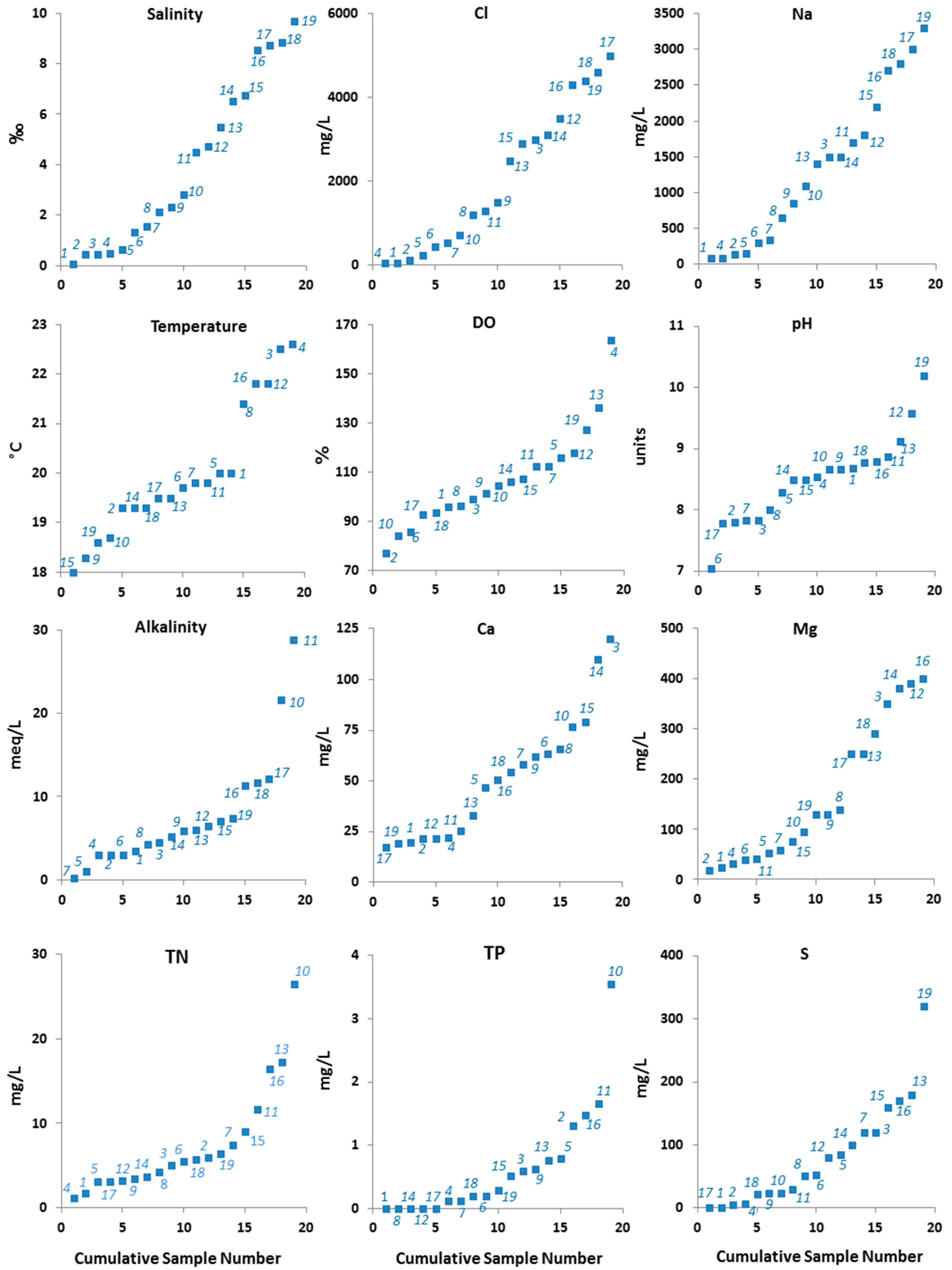
| Parameters | Minimum | Maximum | Mean | Standard Deviation | Skewness |
|---|---|---|---|---|---|
| Salinity (‰) | 0.5 | 10.2 | 4.2 | 3.5 | 0.5 |
| EC (μS/cm) | 0.7 | 15.9 | 6.6 | 5.4 | 0.5 |
| DO (%) | 77.1 | 163.4 | 106.6 | 20.1 | 1.2 |
| pH (pH units) | 7.0 | 10.2 | 8.5 | 0.7 | 0.4 |
| Temperature (°C) | 18.0 | 22.6 | 20.0 | 1.4 | 0.7 |
| Alkalinity (meq/L) | 0.2 | 28.8 | 7.7 | 7.1 | 1.9 |
| Cl (mg/L) | 45.1 | 5000.0 | 2076.1 | 1733.6 | 0.3 |
| TN (mg/L) | 1.1 | 26.5 | 7.4 | 6.4 | 1.8 |
| Al (mg/L) | 0.0 | 400.0 | 36.0 | 92.6 | 3.8 |
| Fe (mg/L) | 0.0 | 290.0 | 26.0 | 67.0 | 3.8 |
| Ca (mg/L) | 17.4 | 120.0 | 50.9 | 30.7 | 0.8 |
| K (mg/L) | 5.5 | 140.0 | 48.0 | 40.9 | 1.2 |
| Mg (mg/L) | 18.5 | 400.0 | 165.6 | 138.7 | 0.6 |
| Na (mg/L) | 85.0 | 3300.0 | 1347.8 | 1068.6 | 0.4 |
| TP(mg/L) | 0.0 | 3.5 | 0.6 | 0.9 | 2.3 |
| S (mg/L) | 1.1 | 320.0 | 81.6 | 82.7 | 1.4 |
© 2016 by the authors; licensee MDPI, Basel, Switzerland. This article is an open access article distributed under the terms and conditions of the Creative Commons Attribution (CC-BY) license (http://creativecommons.org/licenses/by/4.0/).
Share and Cite
Cunningham, L.; Tibby, J.; Forrester, S.; Barr, C.; Skjemstad, J. Mid-Infrared Spectroscopy as a Potential Tool for Reconstructing Lake Salinity. Water 2016, 8, 479. https://doi.org/10.3390/w8110479
Cunningham L, Tibby J, Forrester S, Barr C, Skjemstad J. Mid-Infrared Spectroscopy as a Potential Tool for Reconstructing Lake Salinity. Water. 2016; 8(11):479. https://doi.org/10.3390/w8110479
Chicago/Turabian StyleCunningham, Laura, John Tibby, Sean Forrester, Cameron Barr, and Jan Skjemstad. 2016. "Mid-Infrared Spectroscopy as a Potential Tool for Reconstructing Lake Salinity" Water 8, no. 11: 479. https://doi.org/10.3390/w8110479