
Investigating Alternative Climate Data Sources for Hydrological Simulations in the Upstream of the Amu Darya River


Abstract
:1. Introduction
2. Materials
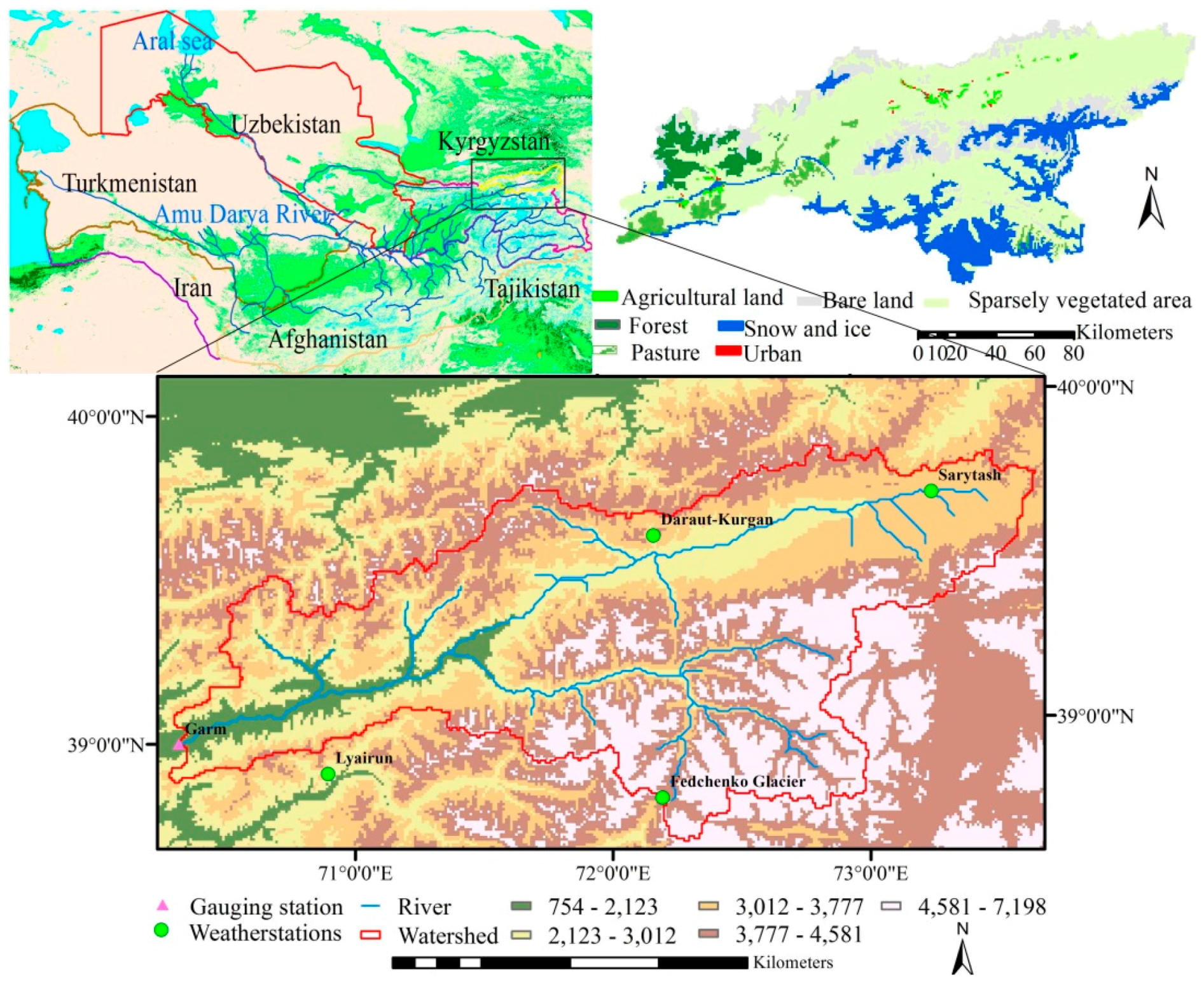
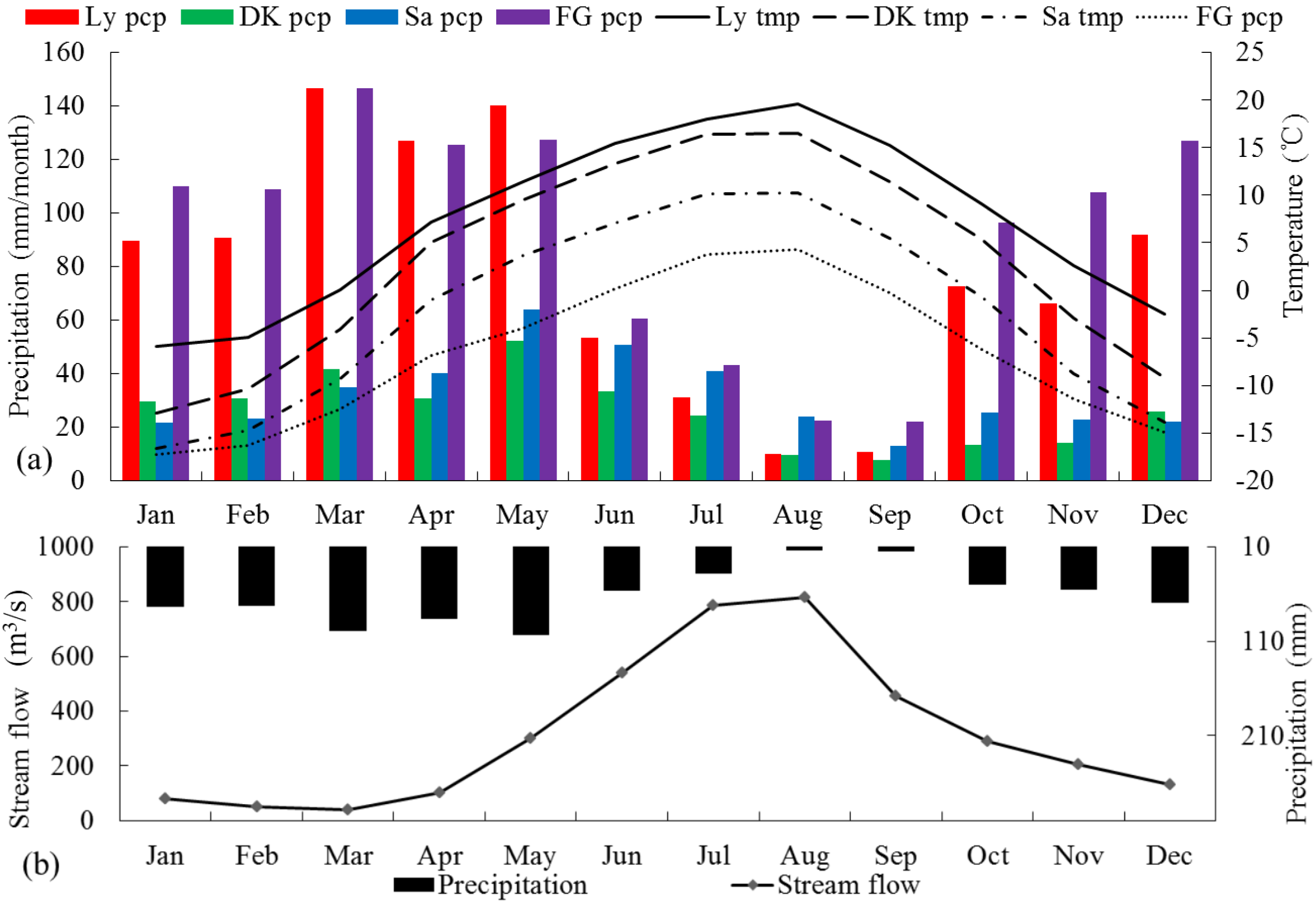
2.1. Study Area
2.2. Data
2.2.1. Climate Data Sources
2.2.2. Other Data for Model Construction
3. Methodology
3.1. Accuracy Assessments of the Grid-Based Data Sets
3.2. Data Correction and Combinations
3.3. The SWAT Hydrological Model
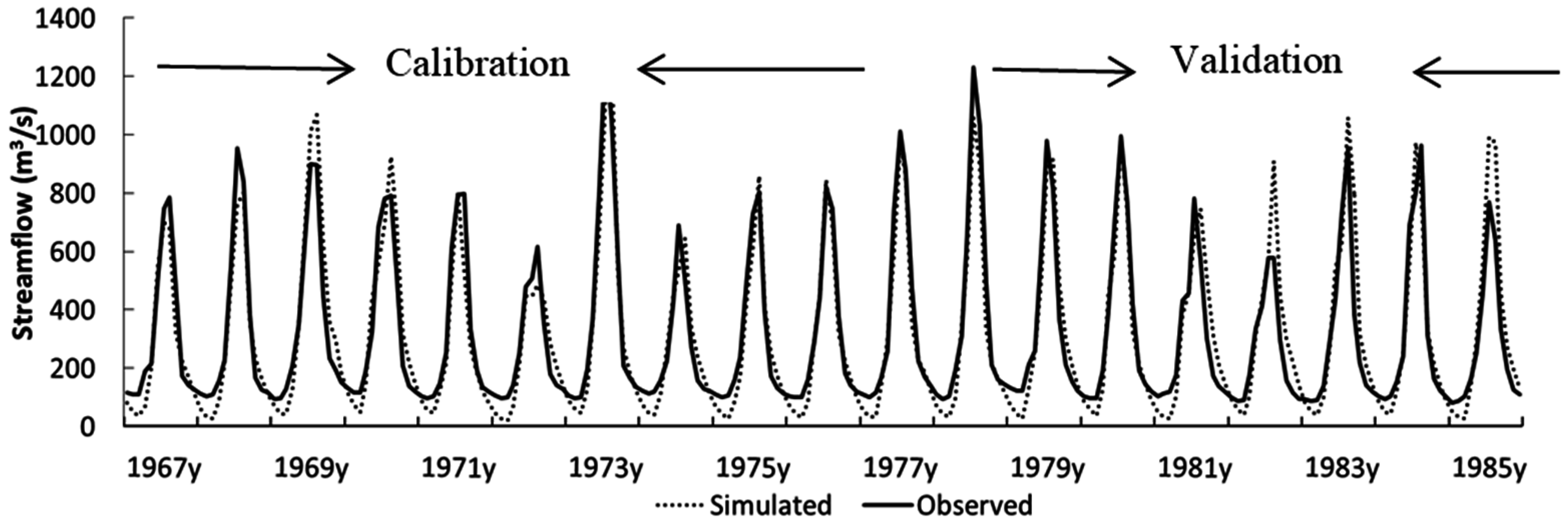
3.4. Model Calibration and Validation
4. Results
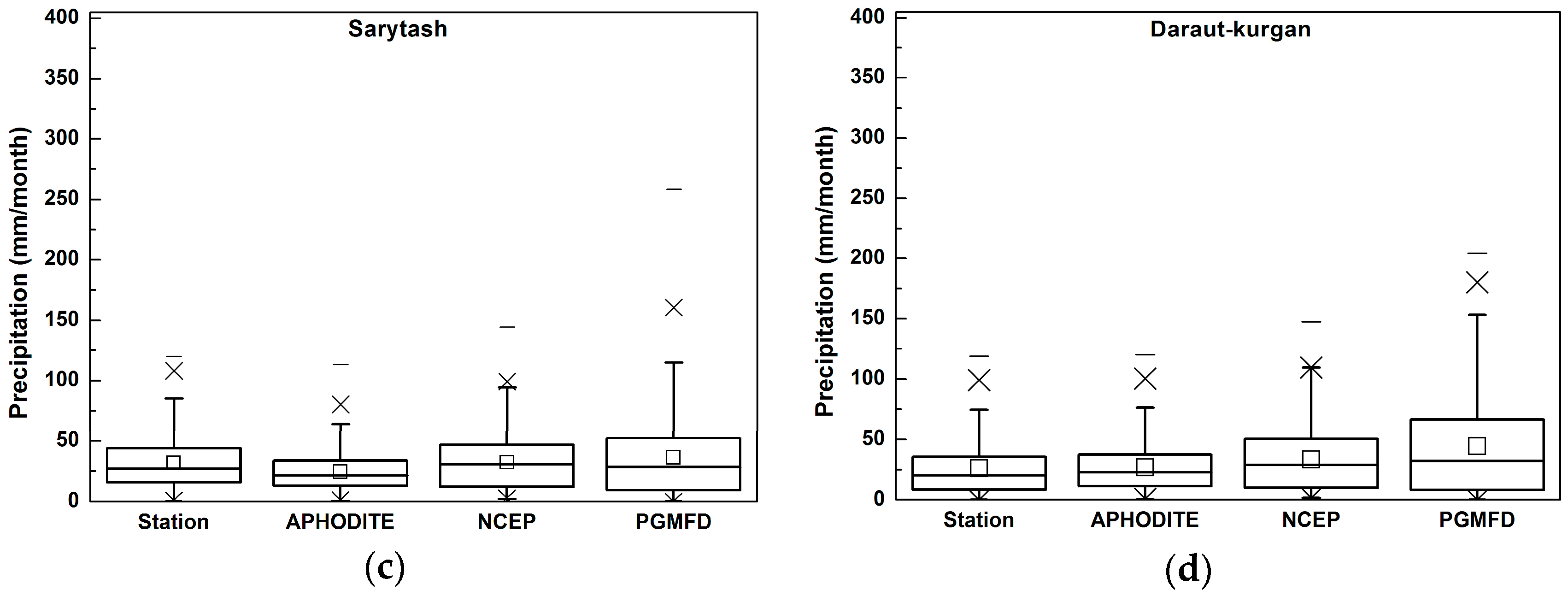
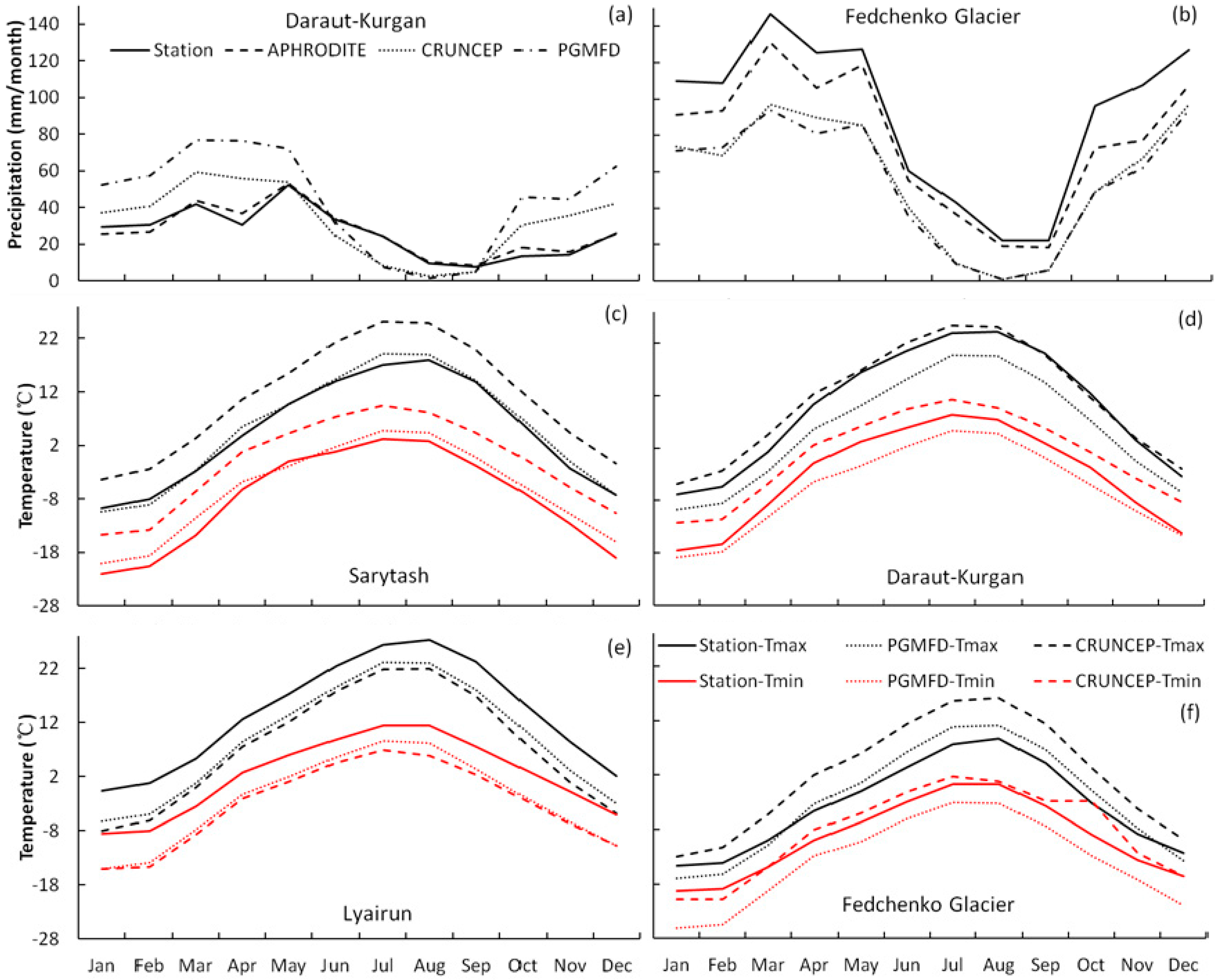
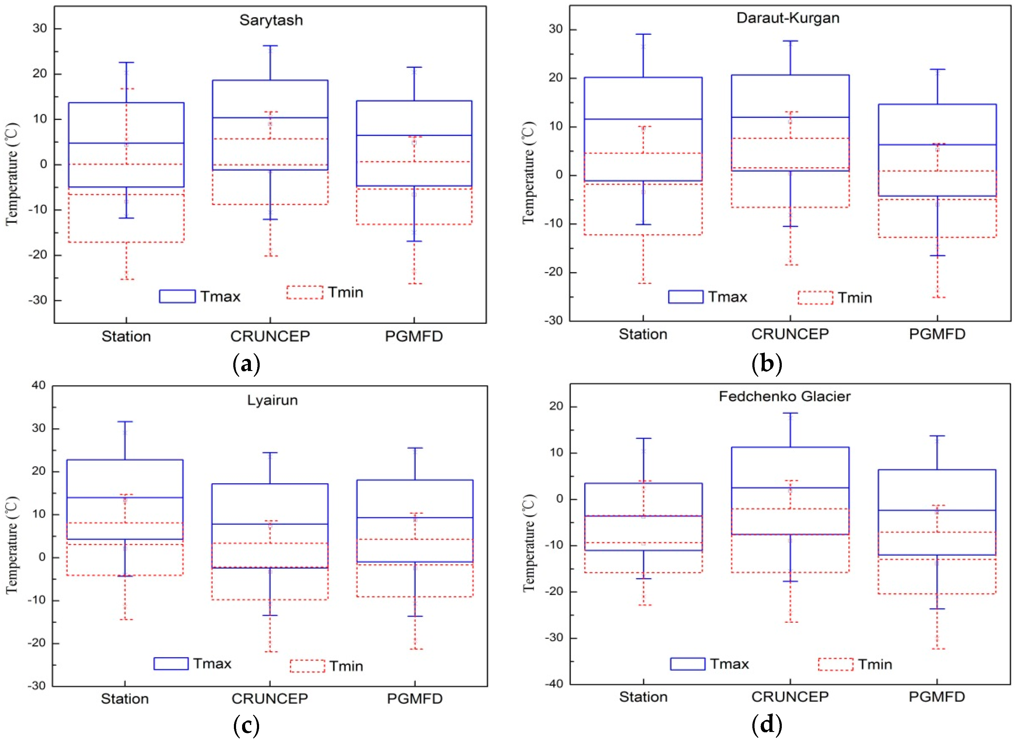
4.1. Evaluation of Data Accuracy
4.2. Modeling River Flow Using Corrected Data
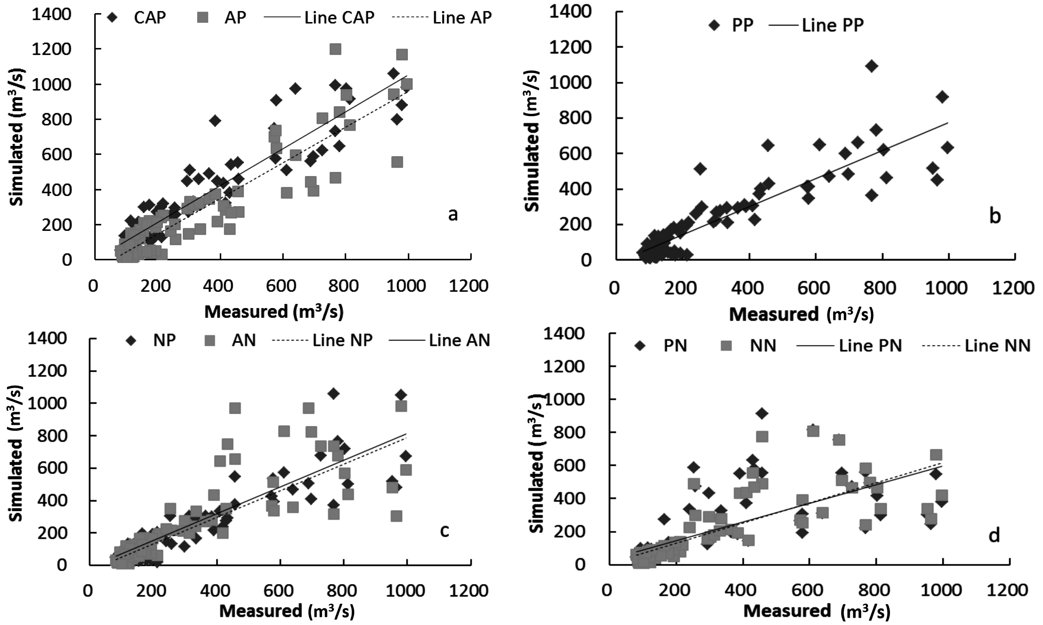
4.3. Modeling River Flow Using Different Data Combinations
5. Discussion
6. Conclusions
Acknowledgments
Author Contributions
Conflicts of Interest
References
- Kouwen, N.; Danard, M.; Bingeman, A.; Luo, W.; Seglenieks, F.R.; Soulis, E.D. Case study: Watershed modeling with distributed weather model data. J. Hydrol. Eng. 2005, 10, 23–38. [Google Scholar] [CrossRef]
- Mehta, V.K.; Walter, M.T.; Brooks, E.S.; Steenhuis, T.S.; Walter, M.F.; Johnson, M.; Boll, J.; Thongs, D. Application of smr to modeling watersheds in the catskill mountains. Environ. Model. Assess. 2004, 9, 77–89. [Google Scholar] [CrossRef]
- Obled, C.; Wendling, J.; Beven, K. The sensitivity of hydrological models to spatial rainfall patterns: An evaluation using observed data. J. Hydrol. 1994, 159, 305–333. [Google Scholar] [CrossRef]
- Bleecker, M.; Degloria, S.D. Mapping atrazine leaching potential with integrated environmental databases and simulation models. J. Soil Water Conserv. 1995, 50, 388–394. [Google Scholar]
- El-Sadek, A.; Bleiweiss, M.; Shukla, M.; Guldan, S.; Fernald, A. Alternative climate data sources for distributed hydrological modeling on a daily time step. Hydrol. Process. 2011, 25, 1542–1557. [Google Scholar] [CrossRef]
- Shrestha, R.; Tachikawa, Y.; Takara, K. Performance analysis of different meteorological data and resolutions using mascod hydrological model. Hydrol. Process. 2004, 18, 3169–3187. [Google Scholar] [CrossRef]
- Schuol, J.; Abbaspour, K.C. Using monthly weather statistics to generate daily data in a swat model application to west Africa. Ecol. Model. 2007, 201, 301–311. [Google Scholar] [CrossRef]
- Immerzeel, W.W.; Droogers, P.; Lutz, A.F. Climate Change Impacts on the Upstream Water Resources of the Amu and Syr Darya River Basins; FutureWater: Wageningen, The Netherlands, 2012. [Google Scholar]
- White, C.J.; Tanton, T.W.; Rycroft, D.W. The impact of climate change on the water resources of the Amu Darya basin in central Asia. Water Resour. Manag. 2014, 28, 5267–5281. [Google Scholar] [CrossRef]
- Ciach, G.J. Local random errors in tipping-bucket rain gauge measurements. J. Atmos. Ocean. Technol. 2010, 20, 752–759. [Google Scholar] [CrossRef]
- Yen, H.; Jeong, J.; Feng, Q.Y.; Deb, D. Assessment of input uncertainty in swat using latent variables. Water Resour. Manag. 2015, 29, 1137–1153. [Google Scholar] [CrossRef]
- Moradkhani, H.; Hsu, K.L.; Gupta, H.; Sorooshian, S. Uncertainty assessment of hydrologic model states and parameters: Sequential data assimilation using the particle filter. Water Resour. Res. 2005, 410, 237–246. [Google Scholar] [CrossRef]
- Hoeting, J.A.; Madigan, D.; Raftery, A.E.; Volinsky, C.T. Bayesian model averaging: A tutorial (with comments by M. Clyde, David Draper and E. I. George, and a rejoinder by the authors. Stat. Sci. 1999, 14, 382–417. [Google Scholar]
- Ajami, N.K.; Duan, Q.; Soroosh, S. An integrated hydrologic bayesian multimodel combination framework: Confronting input, parameter, and model structural uncertainty in hydrologic prediction. Water Resour. Res. 2007, 43, 208–214. [Google Scholar] [CrossRef]
- Bastola, S.; Misra, V. Evaluation of dynamically downscaled reanalysis precipitation data for hydrological application. Hydrol. Process. 2014, 28, 1989–2002. [Google Scholar] [CrossRef]
- Collischonn, B.; Collischonn, W.; Tucci, C.E.M. Daily hydrological modeling in the amazon basin using trmm rainfall estimates. J. Hydrol. 2008, 360, 207–216. [Google Scholar] [CrossRef]
- Duethmann, D.; Zimmer, J.; Gafurov, A.; Güntner, A. Evaluation of areal precipitation estimates based on downscaled reanalysis and station data by hydrological modeling. Hydrol. Earth Syst. Sci. Discuss. 2012, 9, 10719–10773. [Google Scholar] [CrossRef]
- Krogh, S.; Pomeroy, J.W.; Mcphee, J.P. Physically based mountain hydrological modeling using reanalysis data in patagonia. J. Hydrometeorol. 2013, 16, 172–193. [Google Scholar] [CrossRef]
- Li, L.; Hong, Y.; Wang, J.; Adler, R.F.; Policelli, F.S.; Habib, S.; Irwn, D.; Korme, T.; Okello, L. Evaluation of the real-time trmm-based multi-satellite precipitation analysis for an operational flood prediction system in Nzoia Basin, Lake Victoria, Africa. Nat. Hazards 2009, 50, 109–123. [Google Scholar] [CrossRef]
- Li, X.H.; Zhang, Q.; Xu, C.Y. Suitability of the trmm satellite rainfalls in driving a distributed hydrological model for water balance computations in xinjiang catchment, poyang lake basin. J. Hydrol. 2012, 426–427, 28–38. [Google Scholar] [CrossRef]
- Liu, J.; Zhu, A.; Duan, Z. Evaluation of trmm 3b42 precipitation product using rain gauge data in meichuan watershed, Poyang Lake Basin, China. J. Resour. Ecol. 2014, 3, 359–366. [Google Scholar]
- Muñoz, E.; Arum’I, J.L.; Rivera, D.; Montecinos, A.; Álvarez, C. Gridded data for a hydrological model in a scarce-data basin. Water Manag. 2013, 167, 249–258. [Google Scholar] [CrossRef]
- Su, F.; Hong, Y.; Lettenmaier, D.P. Evaluation of trmm multisatellite precipitation analysis (tmpa) and its utility in hydrologic prediction in the la plata basin. J. Hydrometeorol. 2009, 9, 622–640. [Google Scholar] [CrossRef]
- Xue, X.; Hong, Y.; Limaye, A.S.; Gourley, J.J.; Huffman, G.J.; Khan, S.I.; Dorji, C.; Chen, S. Statistical and hydrological evaluation of trmm-based multi-satellite precipitation analysis over the wangchu basin of bhutan: Are the latest satellite precipitation products 3b42v7 ready for use in ungauged basins? J. Hydrol. 2013, 499, 91–99. [Google Scholar] [CrossRef]
- Akurut, M.; Willems, P.; Niwagaba, C.B. Potential impacts of climate change on precipitation over lake victoria, east africa, in the 21st century. Water 2014, 6, 2634–2659. [Google Scholar] [CrossRef] [Green Version]
- Bressiani, D.D.A.; Srinivasan, R.; Jones, C.A.; Mendiondo, E.M. Effects of spatial and temporal weather data resolutions on streamflow modeling of a semi-arid basin, northeast Brazil. Int. J. Agric. Biol. Eng. 2015, 8, 14–25. [Google Scholar]
- Fuka, D.R.; Walter, M.T.; Macalister, C.; Degaetano, A.T.; Steenhuis, T.S.; Easton, Z.M. Using the climate forecast system reanalysis as weather input data for watershed models. Hydrol. Process. 2014, 28, 5613–5623. [Google Scholar] [CrossRef]
- Jajarmizadeh, M.; Sidek, L.M.; Mirzai, M.; Alaghmand, S.; Harun, S.; Majid, M.R. Prediction of surface flow by forcing of climate forecast system reanalysis data. Water Resour. Manag. 2016, 30, 2627–2640. [Google Scholar] [CrossRef]
- Kay, A.L.; Rudd, A.C.; Davies, H.N.; Kendon, E.J.; Jones, R.G. Use of very high resolution climate model data for hydrological modeling: Baseline performance and future flood changes. Clim. Chang. 2015, 133, 1–16. [Google Scholar] [CrossRef]
- Eum, H.I.; Dibike, Y.; Prowse, T.; Bonsal, B. Inter-comparison of high-resolution gridded climate data sets and their implication on hydrological model simulation over the Athabasca Watershed, Canada. Hydrol. Process. 2014, 28, 4250–4271. [Google Scholar] [CrossRef]
- Lauri, H.; Räsänen, T.A.; Kummu, M. Using reanalysis and remotely sensed temperature and precipitation data for hydrological modeling in monsoon climate: Mekong river case study. J. Hydrometeorol. 2014, 15, 1532–1545. [Google Scholar] [CrossRef]
- Jiang, S.; Ren, L.; Hong, Y.; Yong, B.; Yang, X.; Yuan, F.; Ma, M. Comprehensive evaluation of multi-satellite precipitation products with a dense rain gauge network and optimally merging their simulated hydrological flows using the bayesian model averaging method. J. Hydrol. 2012, 452–453, 213–225. [Google Scholar] [CrossRef]
- Beek, T.A.D.; Voß, F.; Flörke, M. Modeling the impact of global change on the hydrological system of the aral sea basin. Phys. Chem. Earth A/B/C 2011, 36, 684–695. [Google Scholar] [CrossRef]
- Qi, J.; Kulmatov, R. An overview of environmental issues in central Asia. In Environmental Problems of Central Asia and Their Economic, Social and Security Impacts; Qi, J., Evered, K.T., Eds.; Springer: Dordrecht, The Netherlands, 2008; pp. 3–14. [Google Scholar]
- Jarsjö, J.; Asokan, S.M.; Shibuo, Y.; Destouni, G. Water scarcity in the aral sea drainage basin: Contributions of agricultural irrigation and a changing climate. In Environmental Problems of Central Asia and Their Economic, Social and Security Impacts; Qi, J., Evered, K.T., Eds.; Springer: Dordrecht, The Netherlands, 2008; pp. 99–108. [Google Scholar]
- Su, Y. The Impacts of Climate Changeon River Flow and Riparian Vegetation in the Amu Darya River Delta, Central Asia. Master’s Thesis, Stockholm University, Stockholm, Sweden, 2012. [Google Scholar]
- Kure, S.; Jang, S.; Ohara, N.; Kavvas, M.L.; Chen, Z.Q. Hydrologic impact of regional climate change for the snowfed and glacierfed river basins in the Republic of Tajikistan: Hydrological response of flow to climate change. Hydrol. Process. 2013, 27, 4071–4090. [Google Scholar] [CrossRef]
- Nezlin, N.P.; Kostianoy, A.G.; Lebedev, S.A. Interannual variations of the discharge of amu darya and syr darya estimated from global atmospheric precipitation. J. Mar. Syst. 2004, 47, 67–75. [Google Scholar] [CrossRef]
- Schär, C.; Vasilina, L.; Pertziger, F.; Dirren, S. Seasonal runoff forecasting using precipitation from meteorological data assimilation systems. J. Hydrometeorol. 2004, 5, 959–973. [Google Scholar] [CrossRef]
- Le, T.B.; Sharif, H.O. Modeling the projected changes of river flow in central vietnam under different climate change scenarios. Water 2015, 7, 3579–3598. [Google Scholar] [CrossRef]
- Pechlivanidis, I.; Olsson, J.; Bosshard, T.; Sharma, D.; Sharma, K.C. Multi-basin modeling of future hydrological fluxes in the indian subcontinent. Water 2016, 8, 177. [Google Scholar] [CrossRef]
- Jarvis, A.; Reuter, H.I.; Nelson, A.; Guevara, E. Hole-Filled Srtm for the Globe Version 4. 2008. Available online: http://srtm.csi.cgiar.org (accessed on 30 September 2016).
- Food and Agriculture Organization (FAO); International Institute for Applied Systems Analysis (IIASA); International Soil Reference and Information Center (ISRIC); Institute of Soil Science, Chinese Academy of Sciences (ISSCAS). Harmonized World Soil Database Version 1.2; FAO: Rome, Italy, 2012. [Google Scholar]
- Hu, Z.; Hu, Q.; Zhang, C.; Chen, X.; Li, Q. Evaluation of reanalysis, spatially-interpolated and satellite remotely-sensed precipitation datasets in central Asia. J. Geophys. Res. Atmos. 2016. [Google Scholar] [CrossRef]
- Zhang, X.L.; Peng, Y.; Wang, B.D.; Wang, H.X. Suitability evaluation of precipitation data using SWAT model. Trans. Chin. Soc. Agric. Eng. 2014, 30, 88–96. [Google Scholar]
- Caldwell, P.; Chin, H.N.S.; Bader, D.C.; Bala, G. Evaluation of a wrf dynamical downscaling simulation over California. Clim. Chang. 2009, 95, 499–521. [Google Scholar] [CrossRef]
- Vu, M.T.; Raghavan, S.V.; Liong, S.Y. SWAT use of gridded observations for simulating runoff—A Vietnam river basin study. Hydrol. Earth Syst. Sci. Discuss. 2011, 8, 2801–2811. [Google Scholar] [CrossRef]
- Moazami, S.; Golian, S.; Kavianpour, M.R.; Hong, Y. Comparison of persiann and v7 trmm multi-satellite precipitation analysis (tmpa) products with rain gauge data over Iran. Int. J. Remote Sens. 2013, 34, 8156–8171. [Google Scholar] [CrossRef]
- Xu, H.; Xu, C.Y.; Sælthun, N.R.; Zhou, B.; Xu, Y. Evaluation of reanalysis and satellite-based precipitation datasets in driving hydrological models in a humid region of southern China. Stoch. Environ. Res. Risk Assess. 2015, 29, 2003–2020. [Google Scholar] [CrossRef]
- Arnold, J.G.; Srinivasan, R.; Muttiah, R.S.; Williams, J.R. Large area hydrologic modeling and assessment part i: Model development. JAWRA 1998, 34, 73–89. [Google Scholar] [CrossRef]
- Srinivasan, R.; Ramanarayanan, T.S.; Arnold, J.G.; Bednarz, S.T. Large area hydrologic modeling and assessment part ii: Model application. JAWRA 1998, 34, 91–101. [Google Scholar] [CrossRef]
- Kiniry, J.R.; Williams, J.R.; King, K.W. Soil and water assessment tool theoretical documentation (version 2005). Comput. Speech Lang. 2005, 24, 289–306. [Google Scholar]
- Gosain, A.K.; Mani, A.; Dwivedi, C. Hydrological Modeling-Literature Review; Climawater Report No. 1; Indian Institute of Technology: Delhi, India, 2009. [Google Scholar]
- USDA Soil Conservation Service. Hydrology. In National Engineering Handbook; Section 4; USDA Soil Conservation Service: Washington, DC, USA, 2010. [Google Scholar]
- Ficklin, D.L.; Zhang, M. A comparison of the curve number and green-ampt models in an agricultural watershed. Trans. Am. Soc. Agric. Biol. Eng. 2013, 56, 61–69. [Google Scholar] [CrossRef]
- Goodrich, D.C.; Keefer, T.O.; Unkrich, C.L.; Nichols, M.H.; Osborn, H.B.; Stone, J.J.; Smith, J.R. Long-term precipitation database, walnut gulch experimental watershed, Arizona, United States. Water Resour. Res. 2008, 44, 570–575. [Google Scholar] [CrossRef]
- Castillo, V.M.; Gómez-Plaza, A.; Martı́Nez-Mena, M. The role of antecedent soil water content in the runoff response of semiarid catchments: A simulation approach. J. Hydrol. 2003, 284, 114–130. [Google Scholar] [CrossRef]
- Zehe, E.; Blöschl, G. Predictability of hydrologic response at the plot and catchment scales: Role of initial conditions. Water Resour. Res. 2004, 40, 497–518. [Google Scholar] [CrossRef]
- Brocca, L.; Melone, F.; Moramarco, T. On the estimation of antecedent wetness conditions in rainfall & ndash; runoff modeling. Hydrol. Process. 2008, 22, 629–642. [Google Scholar]
- Sheikh, V.; Loon, E.V.; Hessel, R.; Jetten, V. Sensitivity of lisem predicted catchment discharge to initial soil moisture content of soil profile. J. Hydrol. 2010, 393, 174–185. [Google Scholar] [CrossRef]
- Hargreaves, G.L.; Hargreaves, G.H.; Riley, J.P. Agricultural benefits for senegal river basin. J. Irrig. Drain. Eng. 1985, 111, 113–124. [Google Scholar] [CrossRef]
- Priestley, C.H.B.; Taylor, R.J. On the assessment of surface heat flux and evaporation using large-scale parameters. Mon. Weather Rev. 1972, 100, 81–92. [Google Scholar] [CrossRef]
- Monteith, J.L. Evaporation and environment. Symp. Soc. Exp. Biol. 1965, 19, 205–234. [Google Scholar] [PubMed]
- Flügel, W.A. Delineating hydrologic response units by geographical information-system analyses for regional hydrological modeling using prms/mms in the drainage-basin of the River Brol, Germany. Hydrol. Process. 1995, 9, 423–436. [Google Scholar] [CrossRef]
- Rodgers, J.L.; Nicewander, W.A. Thirteen ways to look at the correlation coefficient. Am. Stat. 1988, 42, 59–66. [Google Scholar] [CrossRef]
- Yang, Y.; Wang, G.; Wang, L.; Yu, J.; Xu, Z. Evaluation of gridded precipitation data for driving SWAT model in area upstream of three gorges reservoir. PLoS ONE 2014, 9, e112725. [Google Scholar] [CrossRef] [PubMed]
- Ilyas, M.; Shreedhar, M.; Stefan, U.; Vladimir, S. Assessing the impact of areal precipitation input on streamflow simulations using the swat model1. J. Am. Water Resour. Assoc. 2003, 47, 179–195. [Google Scholar]
- Abbaspour, K.C.; Faramarzi, M.; Ghasemi, S.S.; Yang, H. Assessing the impact of climate change on water resources in Iran. Water Resour. Res. 2009, 45, W10434–W10435. [Google Scholar] [CrossRef]
- Abbaspour, K.C.; Yang, J.; Maximov, I.; Siber, R.; Bogner, K.; Mieleitner, J.; Zobrist, J.; Srinivasan, R. Modeling hydrology and water quality in the pre-alpine/alpine thur watershed using swat. J. Hydrol. 2007, 333, 413–430. [Google Scholar] [CrossRef]
- Azimi, M.; Heshmati, G.A.; Farahpour, M.; Faramarzi, M.; Abbaspour, K.C. Modeling the impact of rangeland management on forage production of sagebrush species in arid and semi-arid regions of Iran. Ecol. Model. 2013, 250, 1–14. [Google Scholar] [CrossRef]
- Faramarzi, M.; Abbaspour, K.C.; Schulin, R.; Yang, H. Modeling blue and green water resources availability in Iran. Hydrol. Process. 2009, 23, 486–501. [Google Scholar] [CrossRef]
- Schuol, J.; Abbaspour, K.C.; Srinivasan, R.; Yang, H. Estimation of freshwater availability in the west african sub-continent using the SWAT hydrologic model. J. Hydrol. 2008, 352, 30–49. [Google Scholar] [CrossRef]
- Schuol, J.; Abbaspour, K.C.; Yang, H.; Srinivasan, R.; Zehnder, A.J.B. Modeling blue and green water availability in Africa. Water Resour. Res. 2008, 44, 212–221. [Google Scholar] [CrossRef]
- Gan, R.; Sun, L.; Luo, Y. Baseflow characteristics in alpine rivers—A multi-catchment analysis in northwest China. J. Mt. Sci. 2015, 12, 614–625. [Google Scholar] [CrossRef]


| Data Set | Period | Resolution (°) | Temporal | Region |
|---|---|---|---|---|
| Weather station data | ||||
| CATPD | 1879–2003 | - | monthly | Central Asia |
| GSOD | 1901–2016 | - | daily | Global |
| GHCND | 1763–2016 | - | daily | Global |
| Reanalysis data | ||||
| ERA-15 | 1979–1993 | 2.5 | 6 hourly and monthly | Global |
| NCEP/NCAR | 1948–present | 2.5 | 6 hourly and daily | Global |
| JRA-25 | 1979–2004 | 1.125 | 6 hourly and daily | Global |
| MERRA | 1979–present | 1/2 × 2/3 | hourly | Global |
| CFSR | 1979–present | 0.5 | hourly | Global |
| CRUNCEP | 1948–present | 0.5 | 6 hourly data | Global |
| ERA-Interim | 1979–present | 0.75 | 6 hourly and daily | Global |
| ERA-40 | 1957–2002 | 2.5 | 6 hourly and monthly | Global |
| PGMFD | 1948–2010 | 0.5 | daily | Global |
| GLDAS | 2000–present | 0.25 | 3 hourly | Global |
| Wilmott | 1900–2008 | 0.5 | monthly | Global |
| WFDEI | 1979–2012 | 0.5 | 3 hourly and daily | Global |
| Gridded data | ||||
| APHRODITE | 1951–2007 | 0.25 | daily | Monsoon Asia |
| TRMM | 1998–present | 0.25 | 3 hourly | Near global |
| PERSIANN | 2000–present | 0.25 | 3 hourly | Near global |
| GPCP | 1997–present | 1.00 | daily | Global |
| CMORPH | 2002–present | 0.25 | 3 hourly | Global |
| GSMaP | 2002–present | 0.1 | hourly | 60° N–60° S |
| WFD | 1958–2001 | 0.5 | 3 hourly | Global |
| Station | Statistics | Precipitation | Maximum Temperature | Minimum Temperature | ||||
|---|---|---|---|---|---|---|---|---|
| APHRODITE | CRUNCEP | PGMFD | CRUNCEP | PGMFD | CRUNCEP | PGMFD | ||
| Sarytash | CF (-) | 0.91 | 0.50 | 0.46 | 0.99 | 0.99 | 0.98 | 0.98 |
| RMSE (mm, °C) | 12.19 | 22.52 | 31.7 | 5.02 | 1.72 | 7.07 | 2.55 | |
| MAE (mm, °C) | 8.89 | 16.92 | 22.64 | 4.65 | 1.35 | 6.85 | 2.06 | |
| MBias (-) | 0.77 | 1.01 | 1.14 | 2.05 | 1.11 | 0.17 | 0.8 | |
| NSE (-) | 0.56 | 0.05 | 0.18 | 0.82 | 0.97 | 0.57 | 0.91 | |
| Daraut-Kurgan | CF (-) | 0.32 | 0.26 | 0.21 | 0.98 | 0.98 | 0.97 | 0.98 |
| RMSE (mm, °C) | 29.87 | 34.03 | 57.21 | 2.49 | 4.88 | 4.45 | 3.30 | |
| MAE (mm, °C) | 22.9 | 26 | 39.02 | 1.91 | 4.49 | 3.91 | 2.93 | |
| MBias (-) | 1.03 | 1.28 | 1.71 | 1.13 | 0.55 | −0.13 | 1.74 | |
| NSE (-) | −0.49 | −0.22 | −0.05 | 0.94 | 0.81 | 0.76 | 0.85 | |
| Lyairun | CF (-) | 0.99 | 0.91 | 0.87 | 0.99 | 0.99 | 0.99 | 0.99 |
| RMSE (mm, °C) | 39.42 | 50.07 | 58.15 | 6.25 | 4.83 | 5.57 | 4.78 | |
| MAE (mm, °C) | 23.94 | 36.84 | 39.64 | 6.04 | 4.66 | 5.44 | 4.55 | |
| MBias (-) | 0.88 | 0.59 | 0.65 | 0.55 | 0.65 | −1.54 | −1.12 | |
| NSE (-) | 0.92 | 0.23 | 0.42 | 0.74 | 0.82 | 0.65 | 0.73 | |
| Fedchen-ko Glacier | CF (-) | 0.89 | 0.88 | 0.73 | 0.99 | 0.99 | 0.99 | 0.99 |
| RMSE (mm, °C) | 41.56 | 58.08 | 62.70 | 6.07 | 2.37 | 1.68 | 4.51 | |
| MAE (mm, °C) | 29.94 | 45.15 | 47.25 | 5.61 | 2.06 | 1.41 | 4.22 | |
| MBias (-) | 0.85 | 0.53 | 0.60 | −0.49 | 0.76 | 0.93 | 1.44 | |
| NSE (-) | 0.64 | −0.06 | 0.11 | 0.73 | 0.94 | 0.95 | 0.75 | |
| Parameter | Description | Default Range | Optimized Range | t-Statistic |
|---|---|---|---|---|
| ALPHA_BF.gw | Base flow alpha factor (1/days) | 0–1 | 0.05–0.15 | 23.84 |
| CH_K2.rte | Effective hydraulic conductivity in the main channel (mm/h) | −0.01–500 | 40–80 | −8.99 |
| HRU_SLP.hru | Average slope steepness (m/m) | 0–1 | 0.2–0.6 | 5.17 |
| SMTMP.bsn | Snow melt base temperature (°C) | −20–20 | 0–3.5 | −4.15 |
| SMFMX.bsn | Maximum melt rate for snow during the year (mm H2O/°C-day) | 0–20 | 3.01–6.5 | 3.54 |
| TIMP.bsn | Snowpack temperature lag factor (-) | 0–12 | 0.4–0.9 | 2.56 |
| GW_DELAY.gw | Groundwater delay (days) | 0–500 | 30–60 | −2.10 |
| SOL_K.sol | Saturated hydraulic conductivity (mm/h) | 0–2000 | 50–800 | 1.75 |
| ESCO.hru | Soil evaporation compensation factor (-) | 0–1 | 0.7–0.99 | 1.67 |
| SFTMP.bsn | Snowmelt base temperature (°C) | −20–20 | 0–5 | −1.18 |
| CN2.mgt | SCS runoff curve number (-) | 35–98 | 72–95 | −1.01 |
| CH_K1.sub | Effective hydraulic conductivity in tributary channels (mm/h) | 0–300 | 36–80 | −0.59 |
| GW_REVAP.gw | Groundwater “revap” coefficient (-) | 0.02–0.2 | 0.02–0.10 | −0.35 |
| SOL_AWC.sol | Available water capacity of the soil layer (mm H2O/mm soil) | 0–1 | 0.1–0.4 | 0.04 |
| Statistics | CAP | AP | PP | NP | AN | PN | NN |
|---|---|---|---|---|---|---|---|
| NSE (-) | 0.83 | 0.77 | 0.7 | 0.71 | 0.58 | 0.30 | 0.43 |
| CF (-) | 0.93 | 0.92 | 0.89 | 0.91 | 0.82 | 0.69 | 0.78 |
© 2016 by the authors; licensee MDPI, Basel, Switzerland. This article is an open access article distributed under the terms and conditions of the Creative Commons Attribution (CC-BY) license (http://creativecommons.org/licenses/by/4.0/).
Share and Cite
Sidike, A.; Chen, X.; Liu, T.; Durdiev, K.; Huang, Y. Investigating Alternative Climate Data Sources for Hydrological Simulations in the Upstream of the Amu Darya River. Water 2016, 8, 441. https://doi.org/10.3390/w8100441
Sidike A, Chen X, Liu T, Durdiev K, Huang Y. Investigating Alternative Climate Data Sources for Hydrological Simulations in the Upstream of the Amu Darya River. Water. 2016; 8(10):441. https://doi.org/10.3390/w8100441
Chicago/Turabian StyleSidike, Ayetiguli, Xi Chen, Tie Liu, Khaydar Durdiev, and Yue Huang. 2016. "Investigating Alternative Climate Data Sources for Hydrological Simulations in the Upstream of the Amu Darya River" Water 8, no. 10: 441. https://doi.org/10.3390/w8100441