Modeling Flow Pattern and Evolution of Meandering Channels with a Nonlinear Model

Abstract

Meander dynamics has been the focus of river engineering for decades; however, it remains a challenge for researchers to precisely replicate natural evolution processes of meandering channels with numerical models due to the high nonlinearity of the governing equations. The present study puts forward a nonlinear model to simulate the flow pattern and evolution of meandering channels. The proposed meander model adopts the nonlinear hydrodynamic submodel developed by Blanckaert and de Vriend, which accounts for the nonlinear interactions between secondary flow and main flow and therefore has no curvature restriction. With the computational flow field, the evolution process of the channel centerline is simulated using the Bank Erosion and Retreat Model (BERM) developed by Chen and Duan. Verification against two laboratory flume experiments indicates the proposed meander model yields satisfactory agreement with the measured data. For comparison, the same experimental cases are also simulated with the linear version of the hydrodynamic submodel. Calculated results show that the flow pattern and meander evolution process predicted by the nonlinear and the linear models are similar for mildly curved channels, whereas they exhibit different characteristics when channel sinuosity becomes relatively high. It is indicated that the nonlinear interactions between main flow and secondary flow prevent the growth of the secondary flow and induce a more uniform transverse velocity profile in high-sinuosity channels, which slows down the evolution process of meandering channels.

1. Introduction

The evolution of meandering channels is a complex geomorphological process driven by the interactions between fluid flow and alluvial channel beds and banks. The frequent occurrences of bank erosion and failure events accompanied with meander evolution have brought serious concerns to river managers since they are potential threats to habitation in riparian zones. Although great efforts have been devoted to meander studies in the past few decades, the dynamics of meander evolution has not yet been fully understood.

Observations in recent flume experiments [1,2,3] have revealed that the flow pattern in a meander bend is closely related to its bed topography including the shallow point bars and deep pools developed near the inner and outer banks, respectively. The topographic steering effect redistributes the downstream velocity and affects the evolution process of the meander bend. However, due to the difficulty in concurrently monitoring the flow pattern and channel migration in the field and laboratories, it remains unclear how fluid flow responds to the deformation of channel beds and in turn affects the evolution process of meandering channels. As the computational power rapidly grows in recent decades, numerical models emerge as economical and useful tools in meander studies, exhibiting its unique advantage in unraveling the complex interactions between fluid flow and alluvial beds. Since the pioneering work of Ikeda et al. [4], considerable efforts have been devoted to the development of reliable numerical models for meander simulations ([5,6,7,8,9,10,11,12], among others). However, it remains a challenge to numerically replicate the natural evolution processes of the meandering channels especially for high-sinuosity channels due to possible strong nonlinear interactions in their evolution processes.

In general, a meander evolution model consists of two major components: (1) a hydrodynamic submodel; and (2) a bank erosion submodel. The hydrodynamic submodel is used to simulate the flow field in the meander bend, given the controlling flow discharge and channel geometry. Although a three-dimensional (3D) hydrodynamic model is feasible in present day, reduced-order models, i.e., one-dimensional (1D) or two-dimensional (2D) models are computationally less expensive and theoretically more insightful by revealing the physical processes such as flow redistribution in meander bends [12]. Johannesson and Parker [8] proposed a widely used quasi-2D hydrodynamic model for sine-generated channels, which was based on the perturbative analysis of their model equations. With a few simplifying assumptions, their model has a simple analytical solution, which was successfully applied in several meander evolution studies [6,13]. Similar models were also proposed by Odgaard [14], Imran et al. [15], Zolezzi and Seminara [9], and many others. These models, usually termed “linear models” due to the omission of high-order nonlinear terms in their model equations, mainly differ from the model of Johannesson and Parker [8] in the choice of eddy viscosity profiles. Blanckaert and de Vriend [11] pointed out that the magnitudes of these high-order nonlinear terms increased sharply with channel curvature, and should not be neglected in the simulation of high-sinuosity meanders. Recently, nonlinear theory and numerical models have been applied by different researchers in the context of meander studies. For example, Camporeale et al. [16] developed a general solution method for the coupling system of the nonlinear flow equations and the Exner equation by extending the formulation of Imran et al. [15], which considered the feedback between the main flow and the secondary currents. Abad et al. [17] proposed the STREMR HySeD model, which was established by coupling the two-dimensional hydrodynamic, sediment transport and bed morphology equations, and simulated the flow and bed evolution in fixed-bank meandering channels. Bolla Pittaluga et al. [18] developed a nonlinear bend instability model for meandering channels, which was able to describe the nonlinear response of the meandering processes to initial small perturbations. Other nonlinear models were also developed by Parker et al. [19], Xu et al. [20] and, undoubtedly, others as well. These models were applied in the modeling study of meander dynamics, which improved our understanding of the nature of meandering evolutions. Blanckaert and de Vriend [5] proposed a nonlinear model for meander flow, which retained the essential terms in order to model the nonlinear behavior of meander flow. Their model was tested against the measured data of several flume experiments, and successfully captured the saturation effect of secondary flow in high-sinuosity meanders. However, these experiments were conducted in laboratory flumes with fixed sidewalls, and the nonlinear model has not been fully justified in channels with erodible bank lines.

The bank erosion module defines the constitutive relationship between flow and stream banks. The classical HIPS model [4] empirically correlates the bank migration rate to the near-bank “excess” flow velocity (difference between the near-bank and cross-sectional average velocity). More sophisticated bank erosion models have also been proposed, which take the influences of other channel factors such as the bank height, bank material, mass failure and vegetation into consideration [20,21,22,23,24,25]. Nonetheless, these models assumed that the channel width held constant during meander evolution, and cannot be applied in simulating the width adjustment. Parker et al. [19] developed a new bank erosion model to replace the HIPS model, which discarded the constant-width assumption and built separate equations to evaluate the migration of the eroding bank and depositing banks. A similar model was employed by Eke et al. [26,27] in modeling the coevolution of the planform and channel with in freely meandering rivers. Duan [28] proposed a new bank erosion model which relates the bank migration rate to the near-bank sediment transport rate, which was in turn determined by the longitudinal gradient of streamwise velocity. Considering most bank erosion processes include both bank-toe erosion and bank failure, this model was later coupled with the parallel retreat assumption of stream banks and named as the Bank Erosion and Retreat Model (BERM) by Chen and Duan [6]. BERM has been successfully integrated into the quasi-two-dimensional linear hydrodynamic model of Johannesson and Parker and applied in several numerical studies including meander bend evolution [6,13] and channel width adjustment [10]. However, it has not been tested in the nonlinear context. Therefore, it is interesting to examine how the nonlinear hydrodynamic model, when coupled with BERM, affects the simulations of the meander evolution process.

The objective of this study is to establish a nonlinear meander evolution model by coupling the nonlinear hydrodynamic model of Blanckaert and de Vriend [5] and BERM of Chen and Duan [6], and to assess its performance in meander evolution simulations. The main focus is to investigate the relative importance of the nonlinear hydrodynamic effect and its morphological implication in meander evolution. A series of classical meander flume experiments will be utilized to test the model. The nonlinear effect of the additional processes considered in the nonlinear model on the flow pattern and evolution process will also be analyzed. The manuscript is organized as follows: Section 2 and Section 3 briefly introduce the mathematical formulations used in the nonlinear meander evolution model and its solution algorithm, respectively. Section 4 reports the simulation results of two classical flume experiments reported in da Silva [29] and Friedkin [30] with the proposed model. A sensitivity analysis of the additional processes considered in the nonlinear model on the representative geometry parameters is given in Section 5. The impact of these nonlinear processes on the simulation of flow pattern and meander evolution processes is also discussed in this section. A summary of major findings in this study is presented in Section 6.

2. Mathematical Model

The governing equations of the proposed model include a transport equation for normalized transverse gradient of flow velocity, and a continuity equation for sediment transport in the s-n curvilinear coordinates. The s-axis (longitudinal) lies along the channel centerline, and the n-axis (transverse) is perpendicular to the centerline and pointing at the left bank. The mathematical formulations are briefly described below.

2.1. Hydrodynamic Submodel

The hydrodynamic submodel computes the two-dimensional distributions of velocity and flow depth [11]. For the sake of simplicity, the present study assumes: (1) the flow discharge is constant; (2) the bed slope is uniform; and (3) the flow is uniform. Under these assumptions, the average velocities and flow depths at all cross sections are equivalent. The two-dimensional depth-averaged conservation equations of mass and momentum in curvilinear coordinate system are expressed as [5]:

$$\frac{1}{1+n/R}\frac{\partial U_{s}h}{\partial s}+\frac{\partial U_{n}h}{\partial n}+\frac{U_{n}h}{\left(1+n/R\right)R}=0$$

(1)

$$\begin{array}{c}\frac{1}{1+n/R}{U}_{s}h\frac{\partial U_s}{\partial s}+U_{n}h\frac{\partial U_s}{\partial n}+\frac{U_s{U}_{n}h}{\left(1+n/R\right)R}\hfill \\ =-\frac{1}{1+n/R}gh\frac{\partial z_s}{\partial s}-\frac{{\tau }_b}{\rho }-\frac{1}{1+n/R}\frac{\partial \langle v_s^{*}{v}_s^{*}\rangle h}{\partial s}-\frac{\partial \langle v_s^{*}{v}_n^{*}\rangle h}{\partial n}+\frac{2\langle v_s^{*}{v}_n^{*}\rangle h}{\left(1+n/R\right)R}\hfill \end{array}$$

(2)

where s, n = longitudinal and transverse coordinates; U_s, U_n = depth-averaged longitudinal and transverse flow velocity, respectively; h = flow depth; R = radius of curvature of the channel centerline; g = gravitational acceleration; z_s = water surface elevation; τ_b = bed shear stress; ρ = fluid density; v_s*, v_n* = residual streamwise and transverse velocity components with reference to their depth-averaged quantities; and <v_s*v_s*>, <v_s*v_n*> = so-called dispersion stresses, which represent the correlation between the residual velocities. The first and the second terms in the right-hand-side (RHS) of Equation (2) represent the influence of water surface gradient and the bed friction force, respectively, whereas the third to the fifth terms represent the influence of nonlinear interactions between longitudinal and transverse velocities. Blanckaert and de Vriend [11] suggested that the influence of the correlation <v_s*v_s*> is not significant, and thus can be neglected. The water surface gradient, the bed shear stress and the velocity correlation <v_s*v_n*> can be modeled as [5]:

$$\frac{\partial z_s}{\partial s}=-\psi C_f\frac{U^2}{gH}+n{F_r}^{2}H\frac{\partial }{\partial s}\left(\frac{1}{R_s}\right)$$

(3)

$$\langle v_s^{*}{v}_n^{*}\rangle =\frac{U^{2}H\langle f_s{f}_n\rangle }{R}{g}_{sn}$$

(4)

$$\frac{{\tau }_b}{\rho h}=\psi C_f{U}^2$$

(5)

where ψ = friction amplification coefficient due to bending effect; C_f = Chezy’s friction coefficient; U, H = width-averaged velocity and flow depth; F_r = Froude number, which is defined as U/(gH)^1/2; R_s = curvature radius of the streamline, which can be approximated by R; <f_sf_n> = shape coefficient defining the average transverse transport of the streamwise quantities; and g_sn = shape coefficient characterizing the transverse distribution of <f_sf_n>, which vanishes at river banks and approaches its maximum at the secondary flow cell. The transport equation for normalized transverse gradient of flow velocity can be derived from the equations presented above. The normalized transverse velocity gradient α_s is defined as:

$${\alpha }_s=\frac{\left(1+n/R\right)R}{U_s}\frac{\partial U_s}{\partial n}$$

(6)

Taking spatial derivative in the longitudinal direction on both sides of Equation (6), we obtain:

$$\frac{\partial }{\partial s}\left(\frac{{\alpha }_s}{\left(1+n/R\right)R}\right)=\frac{1}{U_s}\frac{{\partial }^2{U}_s}{\partial s\partial n}-\frac{{\alpha }_s}{\left(1+n/R\right)R}\frac{1}{U_s}\frac{\partial U_s}{\partial s}$$

(7)

Substituting Equations (1)–(5) into Equation (7) with some tedious yet straightforward manipulations, the transport equation for α_s is derived as:

$$\begin{array}{l}\frac{\partial }{\partial s}\left(\frac{{\alpha }_s}{\left(1+n/R\right)R}\right)=\\ \frac{1}{U_s}\frac{\partial }{\partial n}\left(U_n\frac{{\alpha }_s+1}{R}\right)+\frac{{\alpha }_s}{\left(1+n/R\right)R}\frac{{\alpha }_s+1}{R}\frac{U_n}{U_s}-\frac{g}{U_s^2}\frac{{\partial }^2{z}_s}{\partial s\partial n}\\ +\frac{2{\alpha }_s}{\left(1+n/R\right)R}\frac{g}{U_s^2}\frac{\partial z_s}{\partial s}+\left(1+n/R\right)\frac{\psi C_f}{h}\left[\frac{1}{h}\frac{\partial h}{\partial n}-\frac{1}{\left(1+n/R\right)R}\right]\\ +\frac{U^{2}H\langle f_s{f}_n\rangle }{U_s^{2}R}{g}_{sn}\left[\frac{2{\alpha }_s-1}{R}{g}_{sn}\left(\frac{1}{g_{sn}}\frac{\partial g_{sn}}{\partial n}+\frac{1}{h}\frac{\partial h}{\partial n}+\frac{2}{\left(1+n/R\right)R}\right)\right]\\ -\frac{U^{2}H\langle f_s{f}_n\rangle }{U_s^{2}R}\left(1+n/R\right)\frac{\partial }{\partial n}\left[g_{sn}\left(\frac{1}{g_{sn}}\frac{\partial g_{sn}}{\partial n}+\frac{1}{h}\frac{\partial h}{\partial n}+\frac{2}{\left(1+n/R\right)R}\right)\right]\end{array}$$

(8)

According to Blanckaert and de Vriend [5], the first term represents the effect of the convective transport caused by the cross flow; the second and third terms represents the effect of the longitudinal and transverse gradient of the water surface; the fourth term represents the effect of bed friction force; the fifth term represents the effect of momentum redistribution caused by secondary flow. Equation (8) can be further reduced by averaging over the width to obtain:

$$\begin{array}{l}\frac{\partial }{\partial s}\left(\frac{{\alpha }_s}{R}\right)\\ =\frac{1}{12}\frac{{\alpha }_s+1}{R}\frac{B^2}{R}\frac{\partial }{\partial s}\left(\frac{{\alpha }_s+{F_r}^2+A}{R}\right)-\left(1+\frac{B^2}{6}\frac{2{\alpha }_s-1}{R^2}\right)\frac{\partial }{\partial s}\left(\frac{1}{R}\right)-\frac{2{\alpha }_s}{R}\frac{\psi C_f}{H}\\ +\frac{\psi C_f}{H}\frac{{F_r}^2+A-1}{R}+\frac{2\chi }{3}\frac{H\langle f_s{f}_n\rangle }{R}\left[{\left(\frac{2{\alpha }_s-1}{R}\right)}^2+\frac{1}{R}\frac{F{r}^2+A+2}{R}+\frac{12}{B^2}\right]\end{array}$$

(9)

where A = user-prescribed bed scour factor; and B = channel width. Equation (9) is adopted as the governing equation of the hydrodynamic submodel in the present study. Readers can refer to Blanckaert and de Vriend [5] for more details of the derivation. They suggested the additional energy loss in meander bends was contributed by three mechanisms: (1) the nonuniformity of the depth averaged velocity profiles; (2) the additional bed shear stress caused by deformed velocity distributions induced by secondary flow; and (3) the additional turbulence production due to bending effect. Therefore, the friction amplification coefficient ψ can be computed by:

$$\psi ={\psi }_{{\alpha }_{\mathrm{s}}}{\psi }_{\sec }{\psi }_{\mathrm{tur}}$$

(10)

where ψ_αs, ψ_sec and ψ_tur = friction amplification coefficients due to the velocity profile deformation, the secondary flow and the increased turbulence production, respectively. Blanckaert [31] proposed an analytical expression for ψ_αs, which can be expressed as:

$${\psi }_{{\alpha }_{\mathrm{s}}}=1+\frac{1}{12}\frac{B^2{\alpha }_s}{R^2}\left({\alpha }_s+2\right)$$

(11)

ψ_sec, ψ_tur are graphically determined in Blanckaert and de Vriend [11] as functions of βC_f^0.15, where β = C_f^−0.275(H/R)^0.5(α_s + 1)^0.25 is called the bend parameter. In the present study, two analytical expressions are given to approximate the graphical solutions of ψ_sec and ψ_tur as:

$${\psi }_{\sec }=1+0.52\beta {C_f}^{0.15}\exp \left[-\frac{1}{{(2.6\beta {C_f}^{0.15})}^{1.5}}\right]$$

(12)

$${\psi }_{\mathrm{tur}}=1+2.5\frac{{\kappa }^2{Q}^2}{C_f{R}^2}{\left\{1-\exp \left[-\frac{0.4}{\beta {C_f}^{0.15}\left[{\left(\beta {C_f}^{0.15}\right)}^3+0.25\right]}\right]\right\}}^2$$

(13)

<f_sf_n> are also graphically determined in Blanckaert and de Vriend [11]. The analytical expression to approximate <f_sf_n> is:

$$\langle f_{\mathrm{s}}{f}_{\mathrm{n}}\rangle =\left\{1-\exp \left[-\frac{0.4}{\beta {C_f}^{0.15}\left[{\left(\beta {C_f}^{0.15}\right)}^3+0.25\right]}\right]\right\}\langle f_{\mathrm{s}}{f}_{\mathrm{n}}{\rangle }_0$$

(14)

where <f_sf_n>₀ is the shape coefficient given by the linear model of de Vriend [32], which is computed as:

$${\langle f_{\mathrm{s}}{f}_{\mathrm{n}}\rangle }_0=\frac{8C_f}{\kappa }\exp \left(-3.3{\left(\frac{C_f}{\kappa }\right)}^{\frac{2}{3}}\right)$$

(15)

where κ = von Karman constant. Equation (9) can be rearranged into the relaxation form: (1) to cope with the solution algorithm to be developed in the later section; and (2) to reveal the major driving mechanisms that determine the velocity redistribution process in a meander bend:

$$\lambda \frac{\partial }{\partial s}\left(\frac{{\alpha }_s}{R}\right)+\left(1+\epsilon \right)\frac{{\alpha }_s}{R}=F$$

(16)

where

$$\begin{array}{l}\lambda =\frac{1}{2}\frac{H}{\psi C_f}\left(1-\frac{1}{12}\frac{{\alpha }_s+1}{R}\frac{B^2}{R}\right)\\ \epsilon =-\frac{1}{24}\frac{H}{\psi C_f}\left[\frac{B^2}{R}\frac{\partial }{\partial s}\left(\frac{F_r^2+A}{R}-\frac{4}{R}\right)+\frac{32\chi H\langle f_s{f}_n\rangle }{R}\frac{{\alpha }_s-1}{R}\right]\\ F=\frac{1}{2}\frac{F_r^2+A-1}{R}-\frac{1}{2}\frac{H}{\psi C_f}\frac{\partial }{\partial s}\left(\frac{1}{R}\right)\left(1-\frac{B^2}{6R}\right)\\ +\frac{4\chi }{\psi C_f}\frac{H^2}{B^2}\frac{\langle f_s{f}_n\rangle }{R}\left[1+\frac{1}{12}\frac{\left(F_r^2+A+3\right)B^2}{R^2}\right]+\frac{1}{24}\frac{H}{\psi C_f}\frac{B^2}{R^2}\frac{\partial }{\partial s}\left(\frac{F_r^2+A}{R}\right)\end{array}$$

In Equation (16), the first term of F represents the effect of transverse water surface and bed slope; the second term represents the effect of channel curvature change; the third term describes the streamwise momentum redistribution by secondary flow; and the fourth term represents the effect of the cross-flow due to changes in transverse water surface and bed slope. Equation (16) is simplified from the two-dimensional depth-averaged flow equations represented by Equations (1) and (2), yet retains all the essential terms quantifying the nonlinear interactions between the streamwise and secondary flow. These terms are of the order (B/R)²/C_f, and are therefore neglected in the first-order linear models based on the perturbation approach. In weakly curved channels where B/R << 1, Equation (16) can be simplified to the following form:

$$\begin{array}{l}\frac{{\alpha }_s}{R}+\frac{1}{2}\frac{H}{\psi C_f}\frac{\partial }{\partial s}\left(\frac{{\alpha }_s}{R}\right)\\ =\frac{1}{2}\frac{F_r^2+A-1}{R}-\frac{1}{2}\frac{H}{\psi C_f}\frac{\partial }{\partial s}\left(\frac{1}{R}\right)+\frac{4\chi }{\psi C_f}\frac{H^2}{B^2}\frac{\langle f_s{f}_n\rangle }{R}\end{array}$$

(17)

where the friction amplification coefficient ψ is equal to unity, and the shape coefficient <f_sf_n> is evaluated with the linear model of de Vriend [32]. The hydrodynamic model represented by Equation (17) is essentially congruent with the perturbation approach and is therefore termed the “linear” model, whereas the model described by Equation (16) is termed the “nonlinear” model in the present study. Blanckaert and de Vriend [11] argued that in strongly curved channels (with relatively high values of B/R) with smooth boundaries (with low values of C_f), these terms could be of similar magnitudes with other driving terms, which might impose a significant impact on flow pattern and its consequential morphological processes in meandering channels. Therefore, the proposed nonlinear model represented by Equation (16) is more physically based, which can be applied in simulating the meandering channels with various sinuosities.

2.2. Bank Erosion Submodel

The bank erosion submodel computes the planar displacement of the channel centerline with prescribed flow condition at each computational time step, from which the new channel centerline can be generated. The mass balance of sediment transport within the control volume in BERM is expressed as [6]:

$$\omega =\frac{1}{h}\left(b\frac{\partial q_s}{\partial s}+q_n\right)$$

(18)

where ω = bank migration rate; h = local flow depth under the bank-full discharge, i.e., h equals the bank height H along the cross section; q_s, q_n = sediment transport rates in the longitudinal and transverse directions, respectively; and b = half width of the channel. Equation (18) indicates that the bank migration (retreat or advance) is attributed by: (1) the unbalanced sediment transport in the longitudinal direction; and (2) the transverse sediment, transported by the secondary flows.

Some meanders tend to maintain roughly constant bankfull widths during evolution [19], which means the migration rates computed by Equation (18) at the inner and the outer banks equal in magnitude but with opposite signs. However, the width adjustment of sinuous channels, especially channel widening is also a common phenomenon in field and laboratories. Therefore, the discharge bisector line (also termed the center streamline in [6]), defined as the line each point of which equally divides the flow discharge Q in half, is critical for estimating the bank migration rates:

$${\displaystyle {\int }_{-\frac{B}{2}}^{n_{DB}}{U}_{s}hdn}={\displaystyle {\int }_{n_{DB}}^{\frac{B}{2}}{U}_{s}hdn}=\frac{1}{2}Q$$

(19)

where n_DB = transverse coordinate of the discharge bisector line. It is assumed that the migration rate of the centerline can be approximated with the average value of the migration rates for the left and the right banks, which can be expressed as:

$$\omega ={\omega }_A=\frac{1}{2}\left({\omega }_L+{\omega }_R\right)$$

(20)

where subscript A denotes the average value; and L, R represent the left and the right banks, respectively. Recent studies on meander models with adjustable channel widths [19,27] suggested that the migrations of the outer and inner banks are controlled by independent mechanisms and should therefore be simulated with different models. The similar idea is also used in the present study: Equation (18) indicates that the bank migration rate in BERM is determined by the local sediment transport rate (and its gradient), which might also vary in space. Therefore, the migration rates of the left and right banks, ω_L and ω_R, are not necessarily equivalent.

The computation of ω_L and ω_R also requires the transverse profiles of flow velocity and flow depth, which can be computed by [12]:

$$U_s\left(n\right)\approx U\left(1+{\alpha }_s\frac{n}{R}\right)$$

(21)

$$h\left(n\right)\approx H\left[1+\left({F_r}^2+A\right)\frac{n}{R}\right]$$

(22)

A sediment transport formula is required to close the bank erosion submodel. A Levy-type equation for bed-load transport [33] is adopted in the present study to calculate the longitudinal sediment transport rate q_s:

$$q_s\left(1-P\right){\rho }_s=2k_{f}D{\left(\frac{U_{\mathrm{s}}}{\sqrt{gh}}\right)}^2\left(U_s-U_c\right){\left(\frac{D}{h}\right)}^{\raisebox{1ex}{$1$}\!\left/ \!\raisebox{-1ex}{$4$}\right.}$$

(23)

where P = sediment bed porosity; ρ_s = sediment density; k_f = coefficient characterizing the sediment transport intensity; D = representative size of sediment bed; U_c = critical flow velocity for sediment entrainment. Equation (23) is suitable for estimating the sediment transport rate at bed-load dominated streams in sand-bed river (D = 0.25–23 mm). If suspended load transport takes up a large fraction in the total load, an alternative sediment transport should be implemented and tested. The transverse sediment transport rate is related to q_s by:

$$q_n=C_s{q}_s$$

(24)

where C_s = the ratio of transverse to longitudinal sediment transport. Ottevanger et al. [12] argued that the direction of the bed-load transport deviated from the direction of the depth-averaged velocity due to two effects: the uphill pull exerted by the secondary flow and the downhill pull exerted by gravity. They suggested that C_s can be computed by:

$$C_s=\frac{U_n}{U_s}-H\frac{{\alpha }_{\tau }}{R}{g}_{\tau }-G\frac{\partial z_b}{\partial n}$$

(25)

where α_τ denotes the deviation of bed shear stress to depth-averaged flow velocity due to secondary currents; g_τ is a width distribution function; and G is the gravitational pull. It is assumed that C_s along the channel width can be approximated by the value at the centerline, where U_n vanishes at fully developed state [5]. The second term in the RHS of Equation (25) represents the uphill pull by secondary flow, which is computed by [12]:

$$\frac{{\alpha }_{\tau }}{R}={\psi }_{\tau }{\left(\frac{{\alpha }_{\tau }}{R}\right)}_0$$

(26)

where (α_τ/R)₀ represents the linear solution of the deviation of bed shear stress proposed by [32], which is expressed as:

$${\left(\frac{{\alpha }_{\tau }}{R}\right)}_0=\frac{2}{{\kappa }^2}\left(1-\frac{\sqrt{C_f}}{\kappa }\right)\frac{1}{R}$$

(27)

ψ_τ represents the nonlinear correction to the deviation proposed by Blanckaert and de Vriend [11], which is originally graphically determined and can be approximated by an analytical expression as:

$${\psi }_{\tau }=1-\exp \left[-\frac{1}{\beta {C_f}^{0.15}\left(\beta {C_f}^{0.15}+1\right)}\right]$$

(28)

The third term in the RHS of Equation (25) represents the downhill pull by gravity. A gravitational pull model is required to determined the value of G as a function of the dimensionless bed shear stress τ*. Ottevanger et al. [12] reviewed several theoretical gravitational pull models, and compared their performances against the experimental results. In the present study, the Sekine and Parker’s gravitational pull model type ($G~\tau {*}^{0.25}$) [34] was adopted, according to the fit in Ottevanger et al. [12], which can be expressed as:

$$G=0.80\tau {*}^{0.25}$$

(29)

The lateral bed slope əz_b/ən can be related to the bed scour factor A by:

$$\frac{\partial z_b}{\partial n}=H\frac{A}{R}$$

(30)

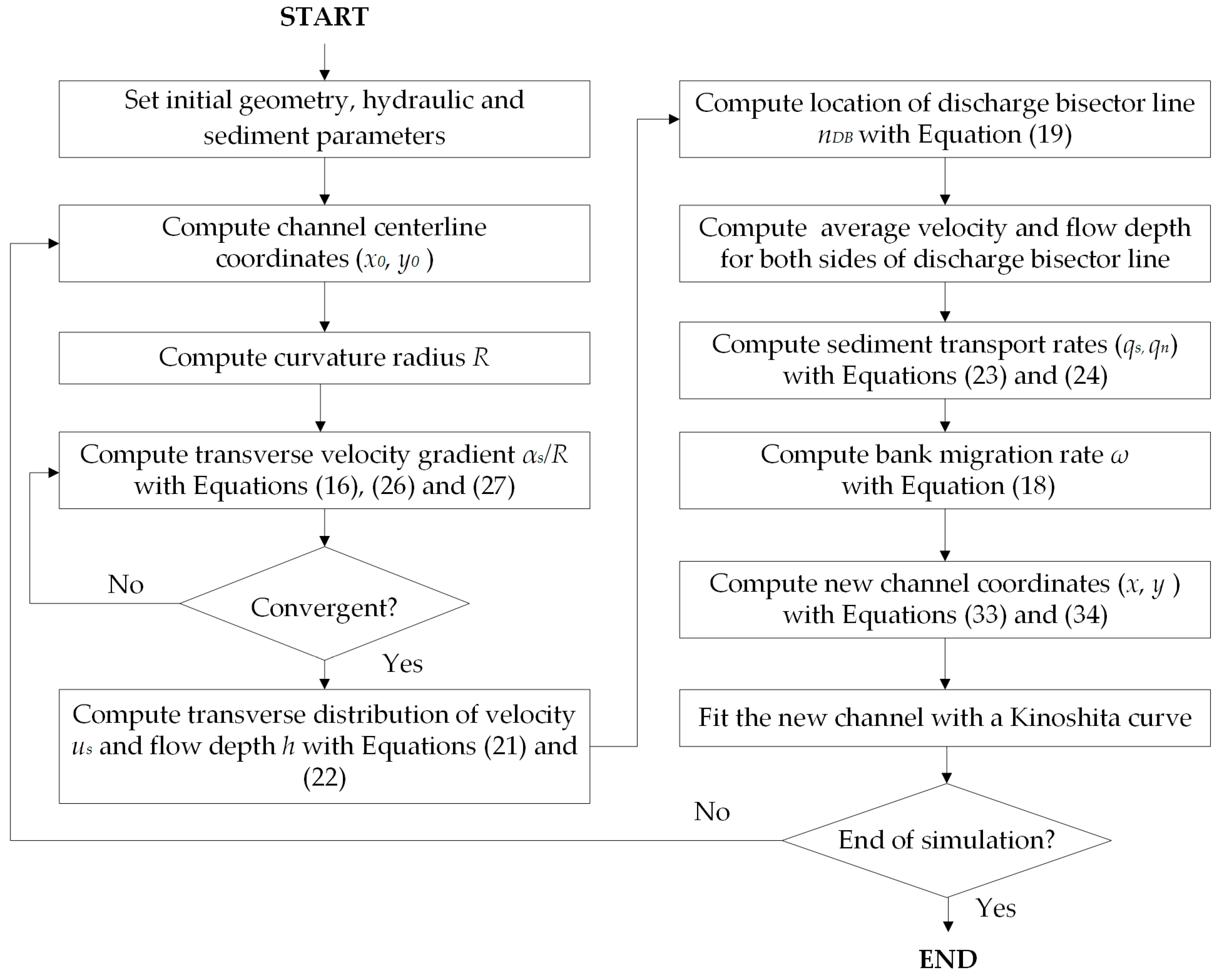
3. Solution Algorithm

Since the morphological time step is usually much larger than the hydraulic time step, the nonlinear model can be solved in a decoupled manner: at each time step, the flow field is computed by solving Equation (16) assuming a rigid channel bed; then the computed flow field is used to compute the longitudinal and transverse sediment transport rates using Equations (23) and (24), and the bank migration rate can be determined by BERM. An implicit scheme is employed in discretizing Equation (16), with the coefficients λ, ε and the source term F evaluated at time level i:

$${\left(\frac{\lambda }{\Delta s}\right)}_{i,j}\left[{\left(\frac{{\alpha }_s}{R}\right)}_{i+1,j+1}-{\left(\frac{{\alpha }_s}{R}\right)}_{i+1,j}\right]+{\left(1+\epsilon \right)}_{i,j}{\left(\frac{{\alpha }_s}{R}\right)}_{i+1,j}=F_{i,j}$$

(31)

where subscript i and i + 1 represent the current and next time levels; j and j + 1 represent the current local and its adjacent nodes; and Δs = grid size. To suppress the instability growth, an under-relaxation iteration scheme is employed:

$${\left(\frac{{\alpha }_s}{R}\right)}_{i+1,j}^{k+1}=\zeta {\left(\frac{{\alpha }_s}{R}\right)}_{i+1,j}^k+\left(1-\zeta \right){\left(\frac{{\alpha }_s}{R}\right)}_{i+1,j}^{k+1,Sol}$$

(32)

where superscript k and k + 1 represent the current and next iteration steps; superscript (k + 1, Sol) represents the value obtained by solving Equation (31); and ζ = under-relaxation factor, which is set to 0.99 in the present study.

After the flow field is determined, the bank migration rate can be calculated by Equations (18) and (20). The new channel after a given time interval Δt is computed using the following expressions:

$$x=x_0+\omega \cdot \Delta t\cdot sin\theta$$

(33)

$$y=y_0+\omega \cdot \Delta t\cdot cos\theta$$

(34)

where x₀, y₀ = Cartesian coordinates of the original channel centerline; x, y = Cartesian coordinates of the channel centerline after the migration; and θ = direction of channel centerline. Equations (33) and (34) implicitly assume that the direction of bank migration is perpendicular to the channel centerline. We herein make an important assumption that the new channel center defined by (x, y) can be approximated with a Kinoshita-type curve [35]. This assumption can effectively suppress the growth of model instability due to strong nonlinearity. Chen and Duan [6] implicitly adopted a similar assumption for the linear hydrodynamic model when they used the analytical solution of Johannesson and Parker [8] to compute the flow velocity distribution. A flow chart summarizing all the steps to perform a full numerical simulation of meander evolution is given in Figure 1.

4. Model Test

4.1. Case 1: Da Silva’s Flume Experiments

Da Silva [29] conducted a series of laboratory meandering flume experiments, two of which were selected in the present study for model validation. The experiments were conducted in two sine-generated flumes with deflection angles (θ₀) of 30° and 110°, respectively (referred to as “S30 case” and “S110 case” hereafter). The meandering channels consisted of two meander loops, which were connected to two straight channels at the upstream and downstream ends as the inflow and outflow channels. The widths of both flumes are 0.4 m with fixed sidewalls, and the meander wavelengths are 2.694 m and 9.298 m, respectively. The sediment bed was immobilized with varnish spray, and the median size of the sediment particles was 2.2 mm. The longitudinal channel bed slopes were 0.001 and 0.00089, respectively, and the transverse channel beds were flat in both cases (A = 0). The flow discharges were kept constant as 2.10 L/s and 2.01 L/s, and the cross-sectional-averaged flow depths were 3.2 cm and 3.0 cm, producing the B/H (width-to-depth ratio) values of 12.5 and 13.3, respectively. The B/H values in the laboratory flumes were usually smaller than those of natural rivers, and caused the effect of the secondary flow to be more pronounced in sharply curved meander bends [5]. Readers can refer to da Silva [29] for more details about the experimental set-ups. Da Silva measured the transverse distributions of flow depth and depth-averaged velocity at 24 selected cross sections, from which the parameter α_s/R can be computed. The experiments were simulated by both the linear and nonlinear models. The effects of the additional nonlinear processes considered in Equation (16) are evaluated via comparison between the computed results and the experimental data.

The longitudinal α_s/R profiles computed from the nonlinear model and the linear model were compared in Figure 2 (S30 case) and Figure 3 (S110 case) with the measured data. It is shown that the α_s/R curves computed from the two models are similar for the S30 case, while significantly differ from each other for the S110 case, especially near the apexes of bends. In the S30 case, the α_s/R profiles computed by both models generally agree with the measured data, although some differences are observed where the streamwise coordinate s is between 2 and 3 m and between 3.5 and 4.5 m, indicating that the advective momentum transport caused by secondary flow is slightly underestimated in these regions. This is possibly because both models describe the transverse distribution of flow velocity by means of a function with only one degree of freedom, represented by Equation (6), which can only approximately represent the real transverse distribution of the velocity. In S110 case, the nonlinear α_s/R profile matches well with the measured data, whereas the linear α_s/R profile is considerably overestimated with a maximum error of 36%. By retaining the additional terms representing the nonlinear hydrodynamic interactions, the nonlinear model produces smaller transverse velocity gradients thus more uniform velocity profiles along the channel width than does the linear model. This is consistent with the assessment of the linear and nonlinear models in previous literature. Blanckaert and de Vriend [5] assessed the performances of the linear and nonlinear models in a sharply curved laboratory channel flume with a 193° bend, and concluded that the linear model significantly overestimated the outward velocity redistribution whereas the nonlinear model adequately captures the α_s/R profile computed from the measured data. Ottevanger et al. [3] also compared the performances of the two models with the Kinoshita laboratory flume experiment of Abad and Garcia [35], the field data of the Polblue Creek in Australia [36], and the Tollense River in Germany [37], and found that the nonlinear model outperformed the linear model in the first two cases with very small B/H (width-to-depth ratio) values, yet both models yield similar results in the third case with relatively larger B/H values. It is indicated that the nonlinear effect is trivial in mildly curved channels, while nonnegligible in strongly curved channels. In general, the α_s/R profiles computed from the nonlinear model, despite some discrepancy at certain locations, generally agree with the measurement, indicating the proposed hydrodynamic submodel is applicable in simulating the flow structures with acceptable accuracy in both the low-sinuosity and high-sinuosity channels.

4.2. Case 2: Friedkin’s Laboratory Experiment

Flume experiments regarding the evolution of meandering channels are not frequently seen in the literature. In the classical flume experiment conducted by Friedkin [30], the channel gradually developed from a mildly curved channel (θ₀ = 30°) into a strongly curved channel (θ₀ > 90°) in 32 h. The locations of the channel talweg were measured in the experiment, which can be used in the present study to test the bank erosion submodel. The width of the channel was 0.64 m, the initial wavelength of the channel (θ₀ = 30°) was 7.62 m, the longitudinal bed slope was 0.0075, the upstream flow discharge was maintained at 0.00283 m³/s, the initial flow depth was 3.0 cm, and the median particle size of the sediment bed was 0.45 mm. The B/H ratio was 21.3, which was generally shallower than the typical values used in laboratory flume experiments (see Ottevanger et al. [3] for example). The transverse channel bed was initially flat at the beginning of the experiment, and gradually developed towards its fully developed state during the experiment. For other details of the experimental set-ups, readers can refer to Chen and Duan [6] or Friedkin [30]. The experiment was simulated with the nonlinear meander model, and the results were compared with the measured data for validation. A computational time step of 8 h for planimetry change is adopted in the simulation; therefore, the planform of channel has been numerically adjusted four times (i.e., at hours 8, 16, 24, and 32). Following Chen and Duan’s work, the transverse bed slope was assumed to increase linearly with time, which reaches the fully developed state at the hour of 32. Therefore, the scour factor A for each time step can be temporally interpolated between zero and its maximum value A_max (see details in Chen and Duan [6]).

The channel centerlines computed by the nonlinear and linear models at each time step were plotted in Figure 4. The measured channel centerline after 32 h of migration was also plotted in the figure for comparison. It is shown that the lengths and widths of the meander bends of the channel centerline predicted by both models are fairly close to those of the measured channel centerline, indicating that the proposed models can at least capture some large-scale geometric properties, such as the average growth rate, of the meander bend in Friedkin’s experiment [30]. Locally, the computed channel centerline evidently deviates from the measured centerline, especially near the third meander apex where the streamwise coordinate s varies between 8 and 12 m. Such deviations between the model results and the experimental data might be caused by two simplifying assumptions adopted in the model: (1) a Kinoshita-type planform with fixed flatness and skewness is imposed to approximate the channel centerline in order to suppress the numerical instability; and (2) the bed scour factor A (linearly related to the transverse bed slope) is prescribed to increase linearly with time during the evolution. These model assumptions might not be realistic in Friedkin’s experiment [30], and should be re-evaluated to allow the meander to evolve freely in future developments of the model.

Since it is the focus of the present study to investigate the relevance of the nonlinear hydrodynamics effects in meander evolution, it is of great interest to analyze the differences of the results predicted by the linear and nonlinear models. It is shown that the channel centerline simulated by the nonlinear model migrates slower than that by the linear model from the downstream of the meander apex to the inflexion point. Such difference could be attributed to the different treatments by the two models in modeling the secondary flow. Blanckaert [31] and Nanson [36] reported that the secondary flow did not increase as the curvature of the channel continues to increase in sharp meander bends, which was referred to as the saturation of the secondary flow. By retaining the additional terms representing the nonlinear hydrodynamic interactions, the nonlinear model limits the growth of the secondary flow, and results in smaller transverse velocity gradients and consequently smaller bank migration rates than the linear model. However, the differences between the two sets of model results are not significant, indicating that the nonlinear effects might not be strong on meander evolution in this experiment possibly due to the relatively large curvature-radius-to-depth ratio (R/H > 77), well exceeding the R/H values found in the test cases of Blanckaert and de Vriend [5] and Ottevanger et al. [3] where the nonlinear effects were much more pronounced in shaping the flow pattern in meander bends. Although the nonlinear effect is not very significant in the present case, the difference between the linear and nonlinear models could accumulate in the long-term simulations of meander evolution and causes significant deviations between their model results. Xu et al. [20] and Bai and Wang [38] suggested that the small perturbations in meandering channels might have long-term effects and eventually developed into large-scale meander bends, which they referred to as “butterfly effect”. Therefore, the long-term effects of the nonlinear hydrodynamic interactions in meander evolution should be further investigated in future studies.

5. Discussion

5.1. Sensitivity of the Nonlinear Terms on Channel Geometry

The terms on the RHS of Equations (16) and (17) quantify the physical processes affecting the simulation of flow pattern in the nonlinear and linear models, respectively. Herein, we use the symbol NT to denote the difference between the RHS terms of Equations (16) and (17):

$$NT=F_N-F_L$$

(35)

where F_N and F_L are the RHS terms of Equations (16) and (17), respectively. It is suggested that NT mainly consists of three components: (1) curvature-induced energy loss; (2) enhanced advective momentum transport by secondary flow; and (3) high-order nonlinear interactions represented by the additional RHS terms in Equation (16). Since these components are inter-correlated, we use NT as the indicator to represent their combined effects. NT was once considered trivial in existing linear meander models, but proven relevant to the flow field in high-sinuosity channels by the simulation of da Silva’s experiment. Therefore, two groups of sensitivity analyses, SA1 and SA2, were conducted to assess the sensitivity of NT on channel sinuosity and its spatial scale. Sine-generated channels with one meander wavelength were employed in the simulation, which was divided into 100 cross sections at equal distance. The channel width, channel slope, and bed material size were kept the same as those used in Friedkin’s experiment. The maximum deflection angle θ₀ and the meander wavelength L were selected as the representative geometry parameters: in SA1, three different deflection angles were used (i.e., θ₀ = 30°, 70° and 110°) to represent mildly, moderately, and strongly curved channels, respectively; in SA2, the meander wavelength was set to be L₀, 2L₀ and 4L₀ (corresponding to L/B = 23.5, 47.1 and 94.1, respectively) to represent channels with different L/B ratios, where L₀ = 15.06 m equals to the channel wavelength (curve length) for θ₀ = 90° in Friedkin’s experiment. Leopold et al. [39] proposed that the meander length is approximately 10 times the channel width based on empirical observations, corresponding to a typical value of L/B = 21.2 for θ₀ = 90°. Although the large L/B values in the latter two scenarios of SA2 are rarely seen in natural rivers, they are selected to evaluate the importance of the nonlinear hydrodynamic effects in channels with different spatial scales. The discharge and flow depth used in the simulations were larger than the actual values deliberately increased to enhance the nonlinear effect so as to make the difference between different scenarios more visible. The detailed parameters settings were listed in

Table 1. Computational parameters used in the sensitivity analysis. Q = discharge; H = flow depth; B = channel width; S = streamwise channel slope; d₅₀ = median particle size of the bed materials; θ₀ = maximum deflection angle; L/B = wavelength-to-width ratio (L is the curve length of the channel within one meander loop).

Parameter	SA1			SA2
	Scenario 1	Scenario 2	Scenario 3	Scenario 1	Scenario 2	Scenario 3
Q (m3/s)	0.02	0.02	0.02	0.02	0.02	0.02
H (m)	0.1	0.1	0.1	0.1	0.1	0.1
B (m)	0.64	0.64	0.64	0.64	0.64	0.64
S (-)	0.0075	0.0075	0.0075	0.0075	0.0075	0.0075
d50 (mm)	0.45	0.45	0.45	0.45	0.45	0.45
θ0 (°)	30	70	110	90	90	90
L/B (-)	23.5	23.5	23.5	23.5	47.1	94.1

.

Figure 5 shows the NT profiles in the meander bend when θ₀ was set to be 30°, 70° and 110°. It is shown that the magnitude of NT increases with θ₀. The value of θ₀ is an indicator of the sinuosity of the channel, which corresponds to different stages of development for an evolving meandering channel. It is indicated that the model error induced by neglecting the nonlinear effect is negligibly small in mildly curved channels (θ₀ = 30°), but gradually accumulates as the curvature effect becomes stronger (θ₀ = 70° and 110°). This characteristic again confirms the findings in Xu et al. [20] that the influence of nonlinearity generally increases with the sinuosity. The difference in the NT magnitudes could well explain the deviation between the linear and nonlinear α_s/R profiles (Figure 2 and Figure 3): as the NT magnitude grows from mildly to sharply curved channels, the error induced by failing to account for the nonlinear hydrodynamic interactions in the linear model also increases and becomes significant in the θ₀ = 110° case. Figure 6 shows the NT profiles when L was set to be L₀, 2L₀ and 4L₀. It is shown that the NT magnitude increases with decreasing L. When θ₀ is fixed, the smaller L corresponds to a meander bend of smaller scale. Therefore, the results suggest that the nonlinear effect is more pronounced for small-scale meandering channels with higher H/R ratios. Xu et al. [20] also analyzed the nonlinear effect in relate to the meander scale, and suggested that smaller river meanders (with larger curvatures) tend to show more influence from the nonlinear consideration. Blanckaert and de Vriend [5] analyzed the relative contributions of different components in the momentum balance as a function of the geometric (width-to-curvature-radius ratio B/R, width-to-depth ratio B/H, roughness C_f) and hydraulic (discharge Q) input variables in sharply curved flume experiments, and found that the nonlinear terms representing the effect of the streamwise variations in curvature and the velocity redistribution by secondary flow are the most important forcing terms in the momentum balance in sharply curved flumes. Ottevanger et al. [3] conducted a similar analysis in a Kinoshita flume and two sharply curved natural rivers, and also confirmed the importance of these processes. They identified the scaling parameter (H/R)/C_f as the major control parameter in determining the magnitudes of the two forcing terms. With all other geometry parameters held constant, the scaling parameter (H/R)/C_f monotonically increases with θ₀ and decreases with L. Therefore, the nonlinear hydrodynamic effect, which increases with increasing θ₀ and decreasing L, could also be scaled by (H/R)/C_f. Both figures show similar spatial profiles along the channel: the NT magnitude approaches its peak value near the meander apex where the channel curvature reaches its maximum value and vanishes in the straight section where the channel curvature decreases to zero, further demonstrating the close relationship between the nonlinear effect and the scaling parameter (H/R)/C_f. Nonetheless, it is also noted that the local extrema of the NT magnitude do not coincide with the apex and inflexion points, owing to the fact that an inertia phase lag is introduced in the numerical model. In summary, the present analysis demonstrates the importance of the nonlinear hydrodynamic effects in the global momentum balance in channels with high sinuosities and low curvature radius, and thus should not be neglected in the numerical simulations of the later stages of meander evolutions for smaller channels.

5.2. Impact of the Nonlinear Terms on Flow Pattern and Meander Evolution

To analyze the effect of the nonlinear processes on meander simulations, the discharge bisector line and the channel centerline after 8 h of migration were compared with the NT magnitude for two sine-generated channels with θ₀ = 30° and θ₀ = 90°. Since it is already shown that the NT magnitude varies with channel sinuosity in the sensitivity analysis, we will continue to examine how such variations would affect the simulated flow pattern and channel evolution.

The magnitudes of the RHS terms, the discharge bisector lines and the channel centerlines after 8 h of migration for θ₀ = 30° and θ₀ = 90° were plotted in Figure 7 and Figure 8. The computed NT magnitudes (represented by the gap between the lines for the nonlinear and linear RHS terms lines in Figure 7 and Figure 8) are substantially larger in the θ₀ = 90° case than in the θ₀ = 30° case. As a result, the differences between the nonlinear and linear discharge bisector lines and channel centerlines are much more pronounced in the former case, indicating that the nonlinear processes substantially affects the simulated flow pattern and the meander evolution process. These additional processes cause the nonlinear discharge bisector line to be closer to the original channel centerline, and the nonlinear channel centerline to migrate slower than its linear counterparts. This is consistent with the findings in Blanckaert and de Vriend [5], who suggested that the nonlinear effect would hinder the growth of the secondary currents and limit the advective momentum transport, resulting in a more uniform transverse distribution of streamwise velocity and thus a smaller longitudinal gradient of flow velocity. Since BERM assumes a linear relationship between the longitudinal velocity gradient and the bank migration rate, both the longitudinal translation and lateral expansion of the simulated new channel computed by the nonlinear model tend to slow down. This conclusion confirms the results in previous literature. Abad et al. [17] employed the STREMR HySeD model, which adopted a correction for secondary flow effects due to streamline curvature, to simulate the bed evolution in a meandering channel and compared the bed evolution patterns simulated with and without the correction. They found that the amount of bed deposition and erosion in the latter case is faster than in the former case. Bai and Wang [38] suggested based on their theoretical model that the stability of the characteristic wave increases with increasing curvature, which indicated that the bend growth was hindered due to increasing nonlinear effects. Eke et al. [27] also reported that the channel migration rate computed by their nonlinear model increased with increasing aspect ratio (width-to-depth ratio), both of which will cause the nonlinear effects to be less pronounced according to the sensitivity analysis in the present study. However, decreasing the wavelength was found to increase the migration rate in their analysis, which seem to contradict with the results in the present study. This is possibly related to the width adjustment process in their simulations, which needs to be further investigated in the future study. From the spatial distributions of the three parameters in a meander bend, it is also noted that the nonlinear effect (indicated by the difference between the nonlinear and linear RHS terms shown by the top plot of Figure 8) is most obvious near the midpoint between the inflexion point and the meander apex, which has an in-phase relationship with the difference between the nonlinear and the linear channel centerlines after migration (shown by the bottom plot of Figure 8), indicating that the simulated channel migration process is strongly affected by the additional processes accounted for in the nonlinear model. Nonetheless, the difference between the nonlinear and linear discharge bisector lines (shown by the mid plot of Figure 8) shows a different spatial distribution, indicating that the influence of the nonlinear processes on the simulated flow pattern is more complex possibly due to the strong three-dimensional characteristics of meander flow.

The differences between the linear and nonlinear results have important implications for meander evolution simulations. The linear hydrodynamic model only provides satisfactory results at low sinuosity/curvature, whereas the nonlinear one provides satisfactory results over the entire curvature range. This is important for modeling the planform evolution of natural rivers. In natural rivers, the curvature and sinuosity usually grow due to erosion at the outer bank and deposition at the inner bank until the upstream and downstream limbs of a meander bend meet and a cut-off event occurs that locally re-straightens the river, leading to a new cycle in the river planform evolution. By retaining the additional terms representing the nonlinear hydrodynamic interactions, the nonlinear hydrodynamic will considerably improve the planform evolution in the high curvature/sinuosity phase of this cycle.

5.3. Limitations of the Present Model

The proposed nonlinear model, at its present form, cannot be directly applied in simulating the planform evolution or other long-term morphodynamic processes of natural rivers due to a number of limitations, which should be improved in the future development of the model:

(1)

A Kinoshita-type planform with fixed flatness and skewness is imposed to approximate the channel centerline in order to suppress the numerical instability. This assumption might be the cause for the deviation between the model results and the measured data in Friedkin’s [30] experiment. The assumption should be replaced in order to allow the channel to develop into freely meandering planforms in the future development.

(2)

The present model does not include a cut-off and local re-straightening module, and thus can handle the simulation of meander evolution only up to the incipient neck cut-off. The cut-off will inevitably occur when the channel sinuosity grows until the upstream and downstream limbs are jointed. The modules to describe the occurrences of cut-off events and local re-straightening processes should be incorporated in the model for simulating the long-term river planform dynamics.

(3)

The Levy-type equation adopted in the bed erosion model is an empirical sediment transport equation based on certain datasets, and only accounts for bed-load transport in a certain particle size range. Extension and generalization of the description of sediment transport, including both the bed-load and suspended-load transport, should be considered in the future development for a wider range of applications of meander evolution.

(4)

The width adjustment process is not simulated in the present study. Parker et al. [19] proposed a theoretical framework for meander migration by using separate relations for modeling the migrations of the eroding and depositing banks, which has been successfully applied in [27] in simulating the coevolution of the width and sinuosity of the meandering channels. Due to the importance of the aspect ratio (width-to-depth ratio) in determining the nonlinear dynamics of the meander channel, the effect of width adjustment should be considered in the future development.

Apart from the model limitations, the data collected in Friedkin’s experiment are not ideal for the validation of numerical meander models. Difference can be observed between the centerlines of the two meander loops (Figure 4), possibly because the centerline was actively evolving at the time when the measurements were made. A meander evolution experiment conducted in mobile banks with hydrodynamic and morphodynamic measurements recorded in detail should be extremely helpful in investigating the dynamics of the meander evolution and assessing the performances of the meander evolution models.

6. Conclusions

In the present study, a nonlinear meander evolution model was developed by coupling the hydrodynamic model of Blanckaert and de Vriend [5] and BERM of Chen and Duan [6]. The proposed model was tested with the flume experiments of da Silva [29] and Friedkin [30]. Two groups of sensitivity analyses are conducted to study the covariation of the additional terms considered in the nonlinear model and the channel geometry parameters. The impacts of the nonlinear processes on the simulated flow pattern and meander evolution process are investigated by comparing the discharge bisector lines and the new channel centerlines computed from both the nonlinear and the linear models for two sine-generated channels with different sinuosities. The main findings of this study are:

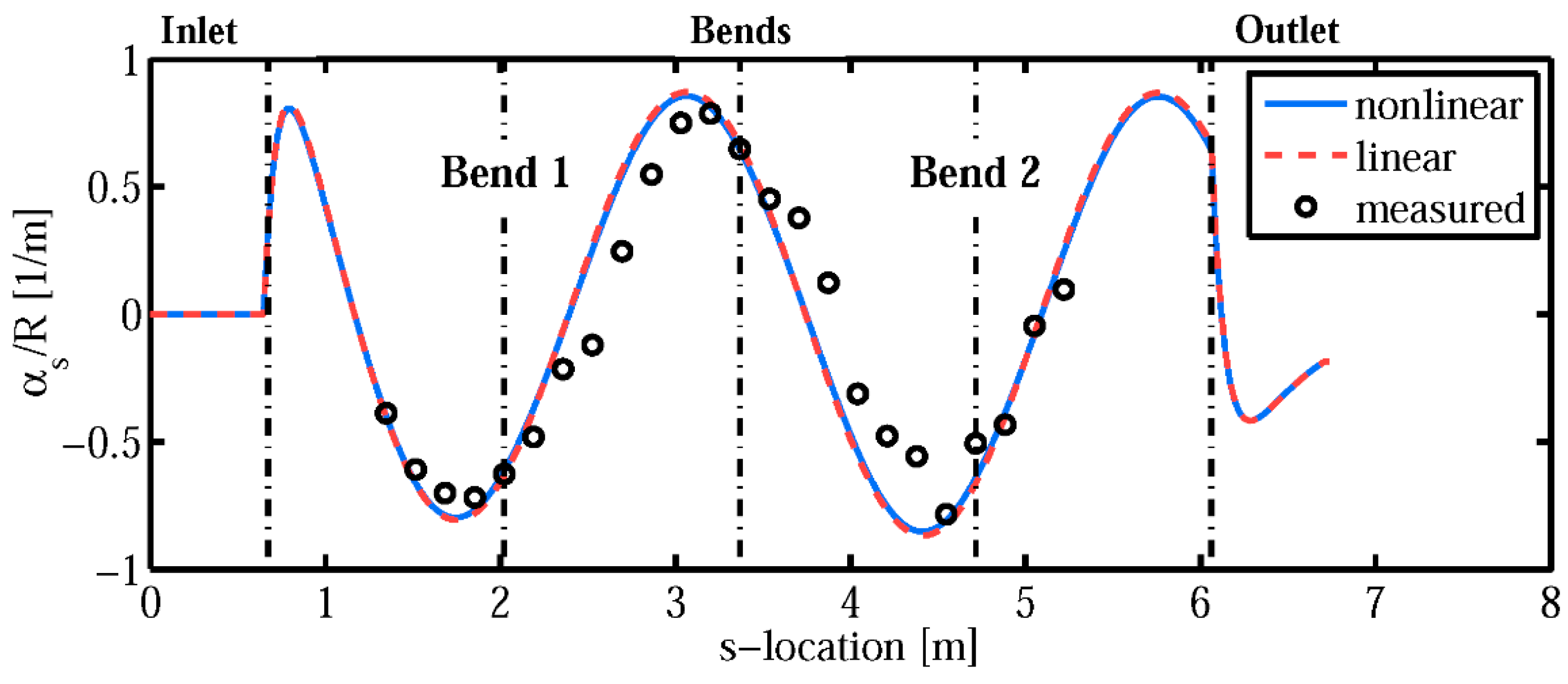
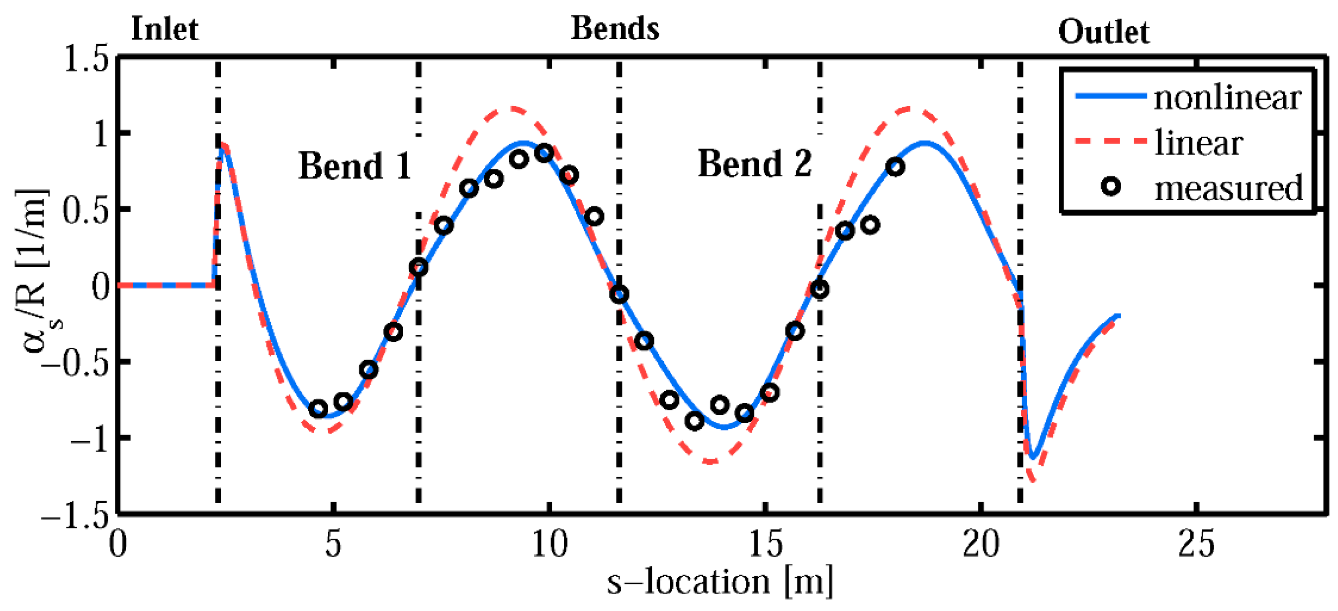
• The proposed nonlinear model is applicable in simulating the flow field and the evolution process of meandering channels with various sinuosities. It is found that the nonlinear effect is trivial in mildly curved channels, but is nonnegligible in strongly curved channels, which is in agreement with the conclusion in Xu et al. [20]. The α_s/R profile computed by both the linear and nonlinear models agree well with the experimental data in da Silva’s 30° experiment [29], whereas the nonlinear α_s/R profile match better with the experimental data than the linear model in da Silva’s 110° experiment, confirming the findings of Blanckaert and de Vriend [5] and Ottevanger et al. [3] that the nonlinear model outperforms the linear model in strongly curved channels.
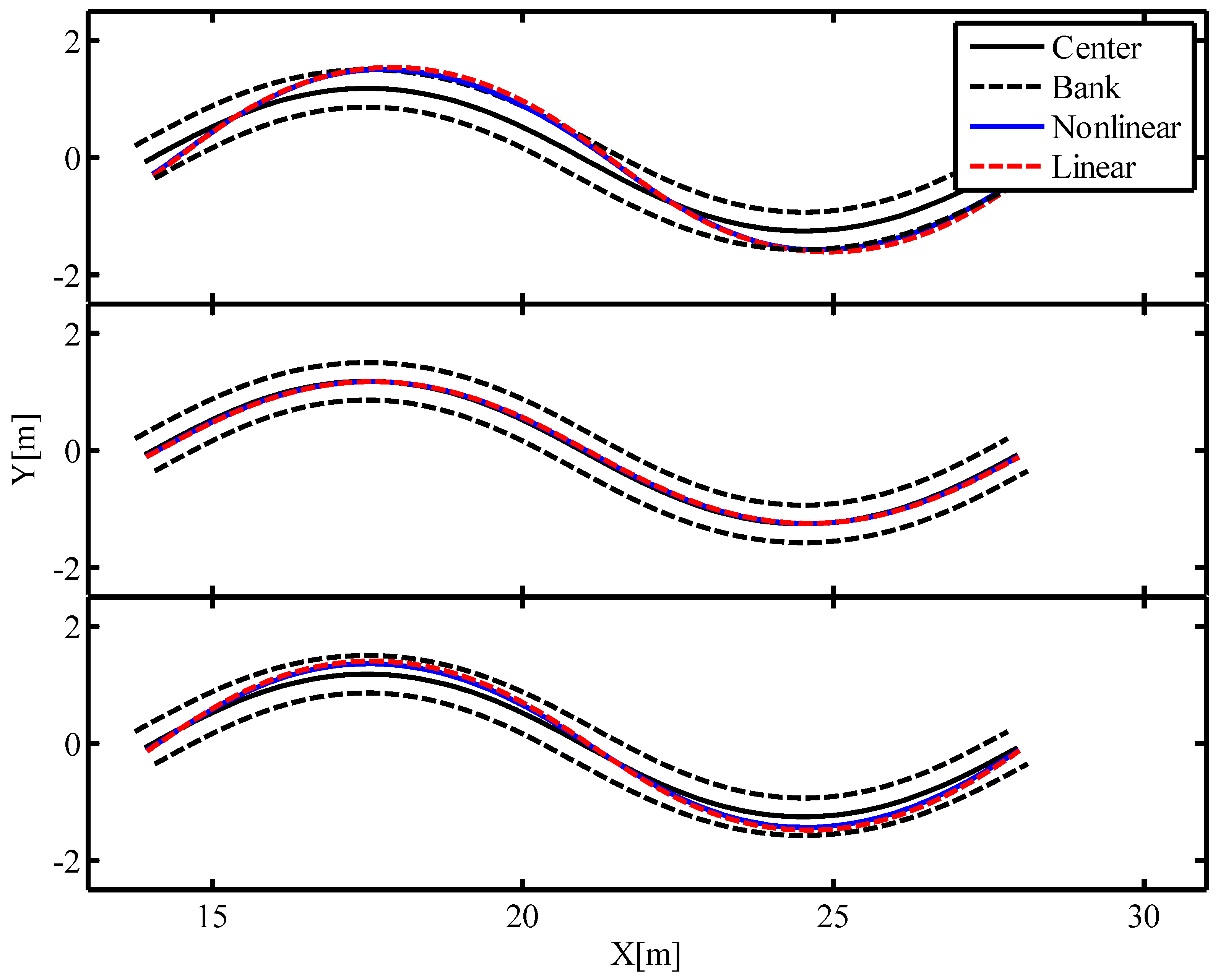
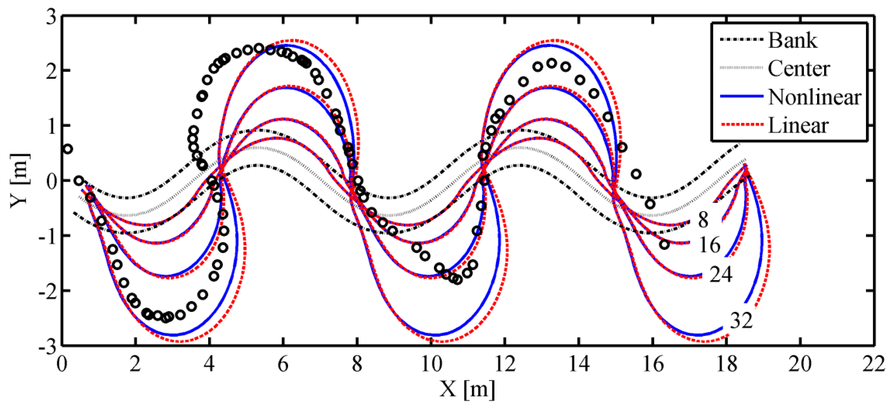
• In the simulation of Friedkin’s experiment [30], the bend growth rates computed by both models generally agree with the measured data, but the computed channel centerlines locally deviate from the measured centerline possibly due to the imposed Kinoshita-type planform and the prescribed bed scour factor. The channel centerline simulated by the nonlinear model migrates slower than that by the linear model in the downstream of the meander apex due to the nonlinear hydrodynamic interactions. However, the difference between the nonlinear and the linear results are not obvious, possibly due to the high width-to-depth ratio in this case.
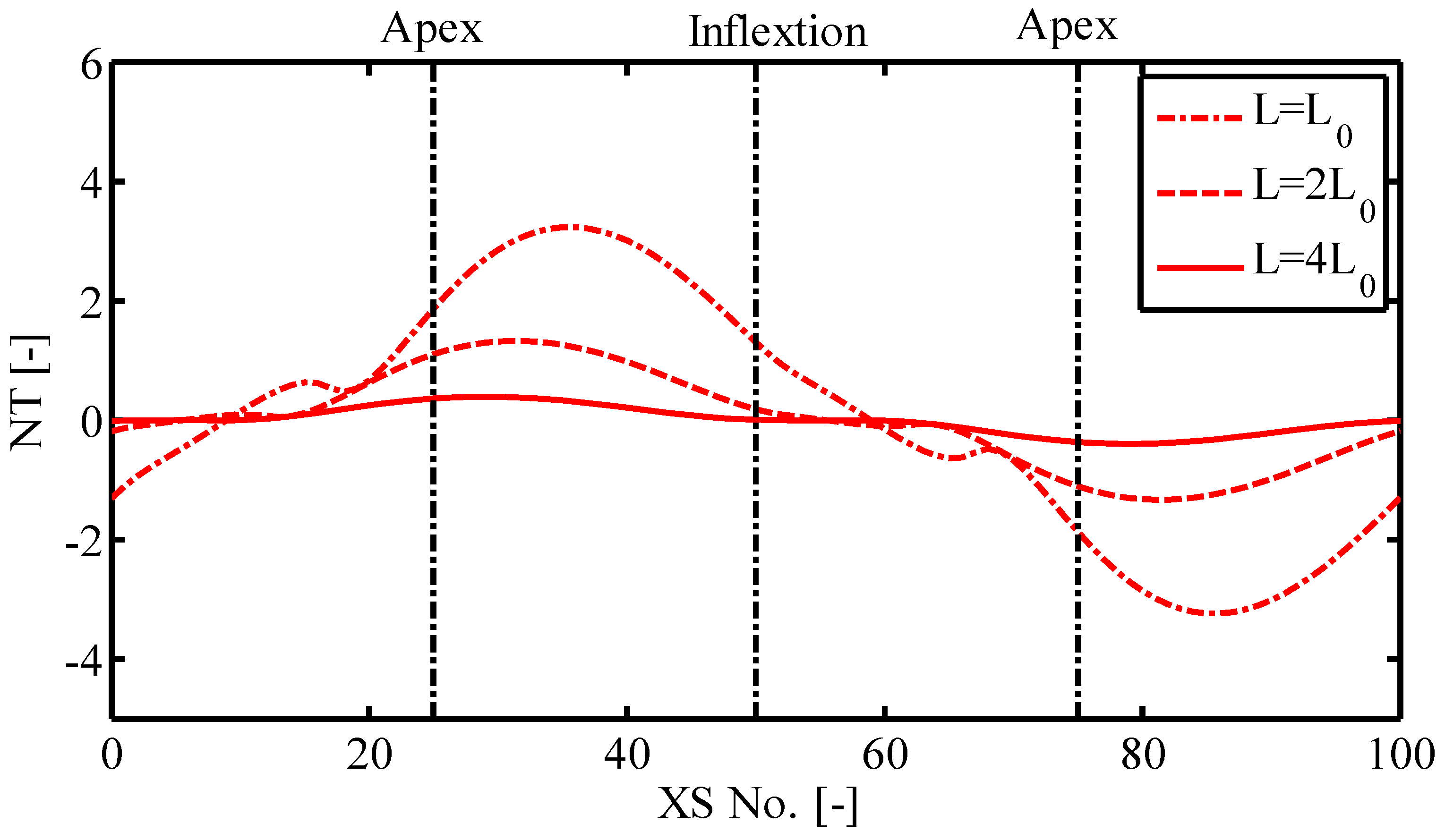
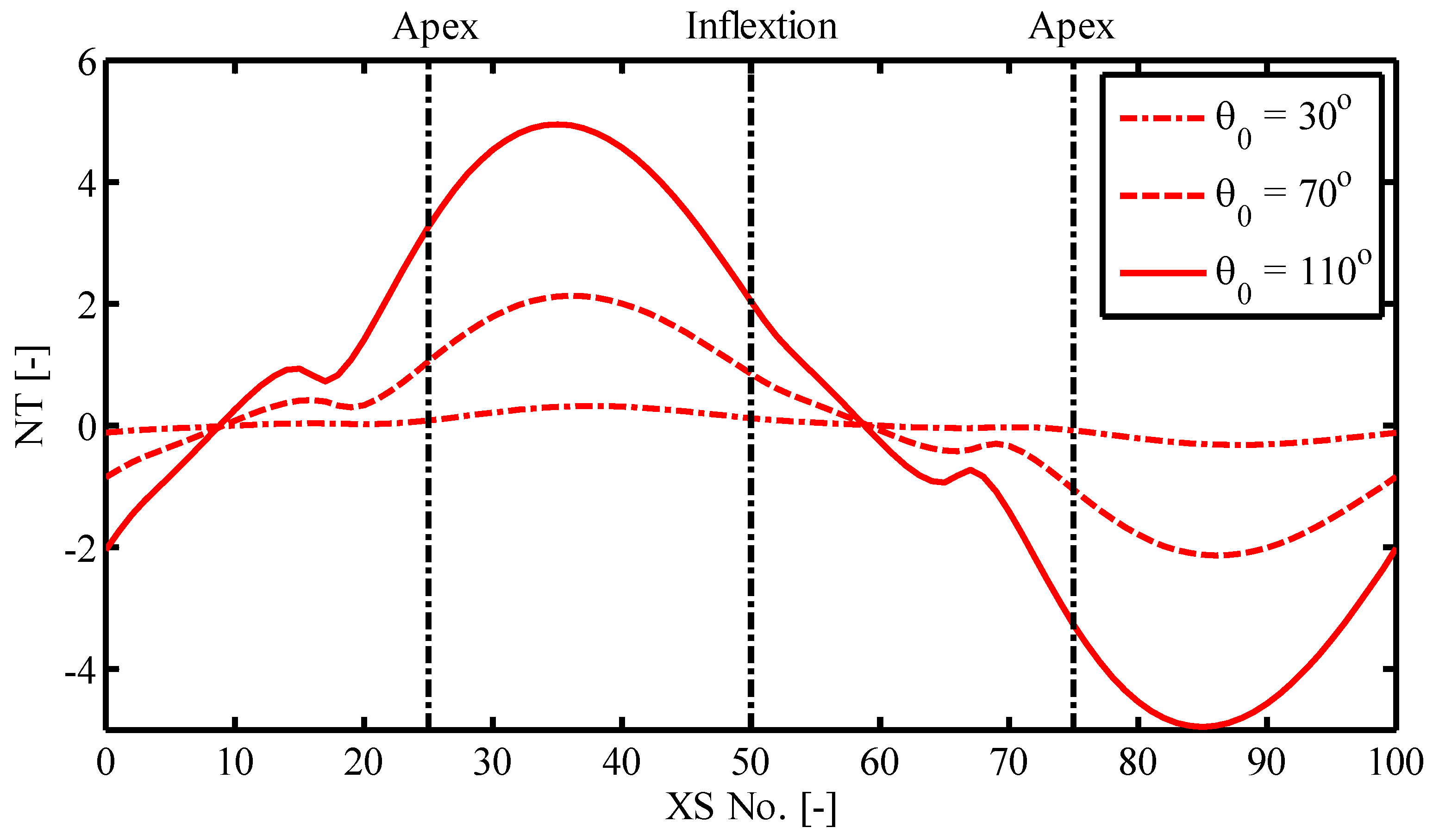
• The sensitivity analysis indicates that the magnitude of the additional terms in the nonlinear model increases with increasing maximum direction angle (sinuosity) and decreasing channel length. This is also consistent with the findings of Xu et al. [20] that the influence of nonlinearity generally increases with sinuosity and decreases with channel scale.
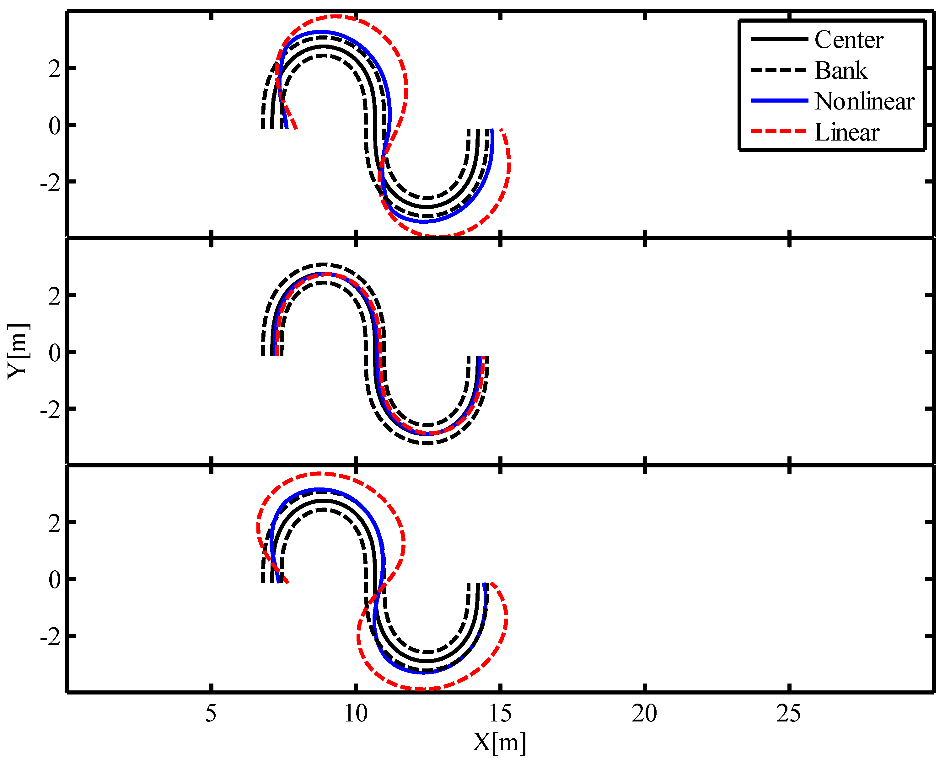
• The additional processes considered in the nonlinear model tend to cause the computed discharge bisector line to be closer to the original channel centerline, and the channel evolution process to slow down. This is in consistent with the findings of Abad et al. [17], Bai and Wang [38], but seemingly contradicts with Eke et al. [27], who reported the migration rate decreased with increasing wavelength possibly because the width adjustment was also simulated in their study. The difference between the nonlinear and linear channel centerlines after migration is in phase with the difference of the nonlinear and linear RHS terms, indicating that the simulated channel migration process is strongly affected by the additional processes accounted for in the nonlinear model. Nonetheless, the difference between the nonlinear and linear discharge bisector lines shows a different spatial distribution, indicating that the influence of the nonlinear processes on the simulated flow pattern is more complex possibly due to the strong three-dimensional characteristics of meander flow.

References

1. Termini, D. Experimental Observations of Flow and Bed Processes in Large-Amplitude Meandering Flume. J. Hydraul. Eng. 2009, 135, 575–587. [Google Scholar] [CrossRef]
2. Blanckaert, K. Topographic steering, flow recirculation, velocity redistribution, and bed topography in sharp meander bends. Water Resour. Res. 2010, 46, 2095–2170. [Google Scholar]
3. Ottevanger, W.; Blanckaert, K.; Uijttewaal, W.S.J. Processes governing the flow redistribution in sharp river bends. Geomorphology 2012, 163–164, 45–55. [Google Scholar] [CrossRef]
4. Ikeda, S.; Parker, G.; Sawai, K. Bend Theory of River Meanders. Part 1. Linear Development. J. Fluid Mech. 1981, 112, 363–377. [Google Scholar] [CrossRef]
5. Blanckaert, K.; de Vriend, H.J. Meander dynamics: A nonlinear model without curvature restrictions for flow in open-channel bends. J. Geophys. Res. 2010, 115, 79–93. [Google Scholar] [CrossRef]
6. Chen, D.; Duan, J.D. Simulating sine-generated meandering channel evolution with an analytical model. J. Hydraul. Res. 2006, 44, 363–373. [Google Scholar] [CrossRef]
7. Blondeaux, P.; Seminara, G. A Unified Bar Bend Theory of River Meanders. J. Fluid Mech. 1985, 157, 449–470. [Google Scholar] [CrossRef]
8. Johannesson, H.; Parker, G. Linear Theory of River Meanders. In River Meandering; Ikeda, S., Parker, G., Eds.; American Geophysical Union: Washington, DC, USA, 1989; pp. 181–213. [Google Scholar]
9. Zolezzi, G.; Seminara, G. Downstream and upstream influence in river meandering. Part 1. General theory and application to overdeepening. J. Fluid Mech. 2001, 438, 183–211. [Google Scholar] [CrossRef]
10. Chen, D.; Duan, J.G. Modeling width adjustment in meandering channels. J. Hydrol. 2006, 321, 59–76. [Google Scholar] [CrossRef]
11. Blanckaert, K.; de Vriend, H.J. Nonlinear modeling of mean flow redistribution in curved open channels. Water Resour. Res. 2003, 39, 1375–1388. [Google Scholar] [CrossRef]
12. Ottevanger, W.; Blanckaert, K.; Uijttewaal, W.S.J.; de Vriend, H.J. Meander dynamics: A reduced-order nonlinear model without curvature restrictions for flow and bed morphology. J. Geophys. Res. 2013, 118, 1118–1131. [Google Scholar] [CrossRef]
13. Chen, D.; Tang, C.L. Evaluating secondary flows in the evolution of sine-generated meanders. Geomorphology 2012, 163–164, 37–44. [Google Scholar] [CrossRef]
14. Odgaard, A.J. River-Meander Model. I: Development. J. Hydraul. Eng. 1989, 115, 1433–1450. [Google Scholar] [CrossRef]
15. Imran, J.; Parker, G.; Pirmez, C. A nonlinear model of flow in meandering submarine and subaerial channels. J. Fluid Mech. 1999, 400, 295–331. [Google Scholar] [CrossRef]
16. Camporeale, C.; Perona, P.; Porporato, A.; Ridolfi, L. Hierarchy of models for meandering rivers and related morphodynmic processes. Rev. Geophys. 2007, 45. [Google Scholar] [CrossRef]
17. Abad, J.D.; Buscaglia, G.C.; Garcia, M.H. 2D stream hydrodynamic, sediment transport and bed morphology model for engineering applications. Hydrol. Process. 2008, 22, 1443–1459. [Google Scholar] [CrossRef]
18. Bolla, P.M.; Nobile, G.; Seminara, G. A nonlinear model for river meandering. Water Resour. Res. 2009, 45, 546–550. [Google Scholar]
19. Parker, G.; Shimizu, Y.; Wilkerson, G.V.; Eke, E.C.; Abad, J.D.; Lauer, J.W.; Paola, C.; Dietrich, W.E.; Voller, V.R. A new framework for modeling the migration of meandering rivers. Earth Surf. Process. Landf. 2011, 36, 70–86. [Google Scholar] [CrossRef]
20. Xu, D.; Bai, Y.C.; Ma, J.M.; Tan, Y. Numerical investigation of long-term planform dynamics and stability of river meandering on fluvial floodplains. Geomorphology 2011, 132, 195–207. [Google Scholar] [CrossRef]
21. Thorne, C.R.; Osman, M.A. The influence of bank stability on regime geometry of natural channels. Int. Conf. River Regime 1988, 18, 135–147. [Google Scholar]
22. Darby, S.E.; Thorne, C.R. Numerical simulation of widening and bed deformation of straight sand-bed rivers. I: Model development. J. Hydraul. Eng. 1996, 122, 184–193. [Google Scholar] [CrossRef]
23. Darby, S.E.; Thorne, C.R.; Simon, A. Numerical simulation of widening and bed deformation of straight sand-bed rivers. II: Model evaluation. J. Hydraul. Eng. 1996, 122, 194–202. [Google Scholar] [CrossRef]
24. Tsujimoto, T. Fluvial processes in streams with vegetation. J. Hydraul. Res. 1999, 37, 789–803. [Google Scholar] [CrossRef]
25. Nagata, N.; Hosoda, T.; Muramoto, Y. Numerical analysis of river channel processes with bank erosion. J. Hydraul. Eng. 2000, 126, 243–252. [Google Scholar] [CrossRef]
26. Eke, E.; Parker, G.; Shimizu, Y. Numerical modeling of erosional and depositional bank processes in migrating river bends with self-formed width: Morphodynamics of bar push and bank pull. J. Geophys. Res. 2014, 119, 1455–1483. [Google Scholar] [CrossRef]
27. Eke, E.C.; Czapiga, M.J.; Viparelli, E.; Shimizu, Y.; Imran, J.; Sun, T.; Parker, G. Coevolution of width and sinuosity in meandering rivers. J. Fluid Mech. 2014, 760, 127–174. [Google Scholar] [CrossRef]
28. Duan, J.D. Simulation of Alluvial Channel Migration Processes with a Two-Dimensional Numerical Model. Ph.D. Thesis, The University of Mississippi, University, MS, USA, 1998. [Google Scholar]
29. Da Silva, A. Turbulent Flow in Sine-Generated Meandering Channel. Ph.D. Thesis, Queen’s University, Kingston, ON, Canada, 1995. [Google Scholar]
30. Friedkin, J. A Laboratory Study of the Meandering of Alluvial Rivers; Technical Reports; U.S. Waterways Experiment Station: Vicksburg, MS, USA, 1945. [Google Scholar]
31. Blanckaert, K. Saturation of curvature-induced secondary flow, energy losses, and turbulence in sharp open-channel bends: Laboratory experiments, analysis, and modeling. J. Geophys. Res. 2009, 114. [Google Scholar] [CrossRef]
32. De Vriend, H.J. A Mathematical Model of Steady Flow in Curved Shallow Channels. J. Hydraul. Res. 1977, 15, 37–54. [Google Scholar] [CrossRef]
33. Chien, N.; Wan, Z. Mechanics of Sediment Transport; ASCE Press: Reston, VA, USA, 1999. [Google Scholar]
34. Sekine, M.; Parker, G. Bed-Load Transport on Transverse Slope. I. J. Hydraul. Eng. 1992, 118, 513–535. [Google Scholar] [CrossRef]
35. Abad, J.D.; Garcia, M.H. Experiments in a high-amplitude Kinoshita meandering channel: 1. Implications of bend orientation on mean and turbulent flow structure. Water Resour. Res. 2009, 45, 325–336. [Google Scholar] [CrossRef]
36. Nanson, R.A. Flow fields in tightly curving meander bends of low width-depth ratio. Earth Surf. Process. Landf. 2010, 35, 119–135. [Google Scholar] [CrossRef]
37. Schnauder, I.; Sukhodolov, A.N. Flow in a tightly curving meander bend: Effects of seasonal changes in aquatic macrophyte cover. Earth Surf. Process. Landf. 2012, 37, 1142–1157. [Google Scholar] [CrossRef]
38. Bai, Y.C.; Wang, Z.Y. Theory and application of nonlinear river dynamics. Int. J. Sediment Res. 2014, 29, 285–303. [Google Scholar] [CrossRef]
39. Leopold, L.B.; Bagnold, R.A.; Wolman, M.G.; Brush, L.M. Flow Resistance in Sinuous or Irregular Channels; Geologic Surey Professional Paper 282-D; U.S. Government Printing Office: Washington, DC, USA, 1960.
Figure 1. Flow chart of performing a numerical simulation with the nonlinear model.
Water 08 00418 g001
Figure 2. The αs/R profiles computed from the nonlinear model (solid line), the linear model (dash line) and the measured data (circles) for the S30 case. The dash-dotted lines indicate the locations of meander apexes.
Water 08 00418 g002
Figure 3. The αs/R profiles computed from the nonlinear model (solid line), the linear model (dash line) and the measured data (circles) for the S110 case. The dash-dotted lines indicate the locations of meander apexes.
Water 08 00418 g003
Figure 4. Comparison of the channel centerlines computed from: (1) the nonlinear model (blue solid line); (2) the linear model (red dash line); and (3) the measured data (circles) for the meander evolution simulations of Friedkin’s experiment. Numbers on the lines indicate the evolution time of the channel.
Water 08 00418 g004
Figure 5. Sensitivity analysis of NT magnitude on the maximum direction angle θ0. NT = the difference between the magnitudes of the RHS terms of Equations (16) and (17); XS No. = cross-section number in the model. The channel starts and ends at the inflexion.
Water 08 00418 g005
Figure 6. Sensitivity analysis of NT magnitude on the meander wavelength L. NT = the difference between the magnitudes of the RHS terms of Equations (16) and (17); XS No. = cross-section number in the model. The channel starts and ends at the inflexion. L0 = characteristic channel length, equivalent to the channel length in Friedkin’s experiment when θ0 = 90° (15.062 m).
Water 08 00418 g006
Figure 7. Comparison of the linear and nonlinear RHS terms (top); the difference between the discharge bisector lines and the original channel centerlines (middle); and the new channel centerlines after 8 h of migration (bottom) computed by the nonlinear and linear models in the θ0 = 30° case.
Water 08 00418 g007
Figure 8. Comparison of the linear and nonlinear RHS terms (top); the difference between the discharge bisector lines and the original channel centerlines (middle); and the new channel centerlines after 8 h of migration (bottom) computed by the nonlinear and linear models in the θ0 = 90° case.
Water 08 00418 g008