Potential Impacts of Climate Change on Water Resources in the Kunhar River Basin, Pakistan

Abstract

Pakistan is one of the most highly water-stressed countries in the world and its water resources are greatly vulnerable to changing climatic conditions. The present study investigates the possible impacts of climate change on the water resources of the Kunhar River basin, Pakistan, under A2 and B2 scenarios of HadCM3, a global climate model. After successful development of the hydrological modeling system (HEC-HMS) for the basin, streamflow was simulated for three future periods (2011–2040, 2041–2070, and 2071–2099) and compared with the baseline period (1961–1990) to explore the changes in different flow indicators such as mean flow, low flow, median flow, high flow, flow duration curves, temporal shift in peaks, and temporal shifts in center-of-volume dates. From the results obtained, an overall increase in mean annual flow was projected in the basin under both A2 and B2 scenarios. However, while summer and autumn showed a noticeable increase in streamflow, spring and winter showed decreased streamflow. High and median flows were predicted to increase, but low flow was projected to decrease in the future under both scenarios. Flow duration curves showed that the probability of occurrence of flow is likely to be more in the future. It was also noted that peaks were predicted to shift from June to July in the future, and the center-of-volume date—the date at which half of the annual flow passes—will be delayed by about 9–17 days in the basin, under both A2 and B2 scenarios. On the whole, the Kunhar basin will face more floods and droughts in the future due to the projected increase in high flow and decrease in low flow and greater temporal and magnitudinal variations in peak flows. These results highlight how important it is to take cognizance of the impact of climate change on water resources in the basin and to formulate suitable policies for the proper utilization and management of these resources.

1. Introduction

The concentration of greenhouse gases (GHGs) has dramatically increased during the last few decades because of anthropogenic forces such as burning of fossil fuels and biomass, land use changes, rapid industrialization, and deforestation. This increased GHGs concentration has resulted in global warming and a global energy imbalance [1,2]. According to the Fifth Assessment Report of the Intergovernmental Panel on Climate Change (IPCC-AR5), the global average temperature has increased by 0.85 °C (0.65 °C–1.06 °C) over the period of 1800–2012, relative to 1961–1990 [3], and 0.74 °C ± 18 °C has been detected during the last hundred years (1906–2005) [4]. There is a very high likelihood of this trend in global warming to only exacerbate. The global average temperature is projected to increase by 1.7 °C–4.8 °C in 2081–2100 (relative to 1986–2005) under different Representative Concentration Pathways (RCPs).

The projected increase in global warming is likely to intensify the hydrological cycle of the world, and hence, disturb the existing hydrological system. As a consequence of global warming, hydrological systems are likely to experience changes in the average availability of water, as well as changes in extreme events such as increase in precipitation intensity, frequency, and/or amount of heavy precipitation [5,6,7]. For example, the average annual precipitation is likely to increase in the high latitudes and the equatorial Pacific Ocean by the end of the 21st century under RCP8.5. However, in several mid-latitude areas and subtropical dry regions, mean precipitation is likely to decrease. The areas of the globe with increasing precipitation are much more than those with decreasing precipitation [3]. This disturbance in a hydrological system can pose problems for public health, industrial and municipal water demand, water energy exploitation, and the ecosystem. However, as stated above, the impact of climate change on hydrological systems may vary from region to region [2,3,5,8].

Hydrological systems are of great importance as they greatly affect the environmental and economic development of a region and are highly complex because they comprise the atmosphere, cryosphere, hydrosphere, biosphere, and geosphere. The hydrological cycle of a basin (catchment) is mainly influenced by the physical characteristics of the basin, climatic conditions in the basin, and human activities. Most studies on climate change have focused on temperature, precipitation, and evaporation [9] since these are considered to be the key indicative factors of climate change and variability in a river basin [10]. There is an increasing consensus that changing trends in climatic variables, especially temperature and precipitation, can change the hydrological and ecological conditions of a river basin [11,12]. Given all these conditions, it is of great importance to assess the possible impacts of climate change on the water resources of a region, which can help in the proper utilization and management of these water resources.

The economy of Pakistan relies greatly on agriculture, which is heavily dependent on the Indus River Irrigation System. Water issues in Pakistan are crucial challenges for the policymakers and managers of water resources in the country [13]. Today, Pakistan is one of the most water-stressed countries in the world as water availability in the country has reduced from about 5000 m³ per capita per year in 1952 to 1100 m³ per capita per year in 2006, which is an alarming situation [14]. According to the United Nations report, a country with water availability of less than 1000 m³ per capita per year is considered a water scarce country [15]. The reduction in water availability has created tensions among different provinces due to the increasingly unequal distribution of water. Climate change and variability are likely to affect water availability for, and magnitude of, irrigation and hydropower production in the country. These changing water conditions are likely to increase the tensions among the provinces, especially at the downstream (Sindh province) [13]. Therefore, a clear estimation of future water resources under changing climatic conditions is of great importance for the planning, operation, and management of hydrological installations in any watershed in Pakistan.

In the last few years, outputs from General Circulation Models (GCMs)—the most advanced and numerical based coupled models—are fed into hydrological models to explore the impacts of climate change on water resources in various parts of the world in the future. However, these models are coarse in spatial resolution (about 200–500 km) [16] and might not be suitable at the basin level, especially small basins which require very fine spatial resolution [17,18]. To bridge GCM resolution and basin scales, downscaling—dynamical and statistical—techniques have been developed. In dynamical downscaling, a high-resolution numerical based Regional Climate Model (RCM), with a resolution of about 5‒50 km, uses the course outputs of a GCM and provides detailed information or high resolution outputs at the basin level [2]. On the other hand, Statistical downscaling (SD) methods (i.e., stochastic weather generator, regression, and weather typing) create empirical/statistical relationships between the GCM scale and basin scale variables (e.g., temperature and precipitation). Compared to dynamical downscaling, SD methods are faster and computationally inexpensive, and thus offer approaches that have been rapidly adopted by a wider community of scientists [17]. For the present study, downscaled data (maximum temperature, minimum temperature, and precipitation) was obtained from [1]. They used a Statistical Downscaling Model (SDSM), a combination of multiple linear regression and a stochastic weather generator, to downscale temperature and precipitation over the period of 2011–2099 under A2 and B2 scenarios of HadCM3, a global climate model.

Different studies such as Akhtar et al. [13], Ahmad et al. [19], Shrestha et al. [20], and Bocchiola et al. [21] have assessed the impacts of climate change on the water resources of Pakistan [13,19,20,21]. These studies were mostly conducted in the Upper Indus basin using hydrological models such as Snowmelt Runoff model (SRM), Hydrologiska Byråns Vattenbalansavdelning (HBV), Soil and Water Assessment Tool (SWAT), and the WEB-DHM-S model. However, to the best of our knowledge, no studies have been conducted to explore the potential impacts of climate change on the water resources of the Kunhar River basin, which is one of the main tributaries of the transboundary Jhelum River and is located entirely in Pakistan. The Kunhar River originates from the Greater Himalayas and contributes to the Mangla Reservoir after joining the Jhelum River. The Mangla Reservoir’s water is used for irrigation and hydropower production. It is the second largest reservoir of Pakistan. Although HEC-HMS, a well-known hydrological model, has been successfully used for small to large and plains to mountainous areas of the world [22,23,24,25,26,27], almost no studies have been reported in Pakistan that use HEC-HMS for the assessment of climate change impacts on water resources.

Thus, the main objectives of the present study were: (1) the development of HEC-HMS, a hydrological model, in the mountainous Kunhar River basin which is greatly influenced by winter snowfall; and (2) to assess the possible impacts of climate change on the water resources of the Kunhar River basin, located in Pakistan, under A2 and B2 scenarios of HadCM3. Description of the data and the study area are given in Section 2 and Section 3 of this paper. A brief introduction of the hydrological model used in the study, and the methods used for the analysis of streamflow, is given in Section 4. Section 5 and Section 6 include the results/discussion and conclusions respectively. This study will be very useful for policies that govern the utilization and management of the water resources of the Kunhar basin, which contributes significantly to the Mangla reservoir, under the effects of climate change.

2. Data Description

2.1. Hydro-Meteorological Data

Observed daily historical data of three climate stations (maximum temperature, minimum temperature, and precipitation) were collected from the Pakistan Meteorological Department (PMD) and the streamflow data of two hydrometric stations, spanning 1961 to 2000, from the Water and Power Development Authority (WAPDA). The geographical and basic information of the hydro-meteorological stations is presented in Table 1 and Figure 1.

Table 1. Basic information about hydro-climatic stations in the Kunhar River basin.

SR	Station	Lat	Long	Altitude	Period	PP	TX	TN
	Meteorological	(° N)	(° E)	(m ASL)	(year)	Annual (mm)	Mean (°C)	Mean (°C)
1	Balakot	34.55	73.35	995	1961–2000	1514	24.9	12.4
2	Muzaffarabad	34.37	73.48	702	1961–2000	1477	28.4	13.5
3	Naran	34.9	73.65	2421	1961–2000	1522	12.3	3.2
						1504	21.8	9.7
	Hydrometric					Mean Discharge		Catchment Area
						Annual (mm)	m3/s	km2
1	Naran	34.90	73.65	2362	1961–2000	1441	47	1011
2	Gari Habibullah	34.40	73.38	810	1961–2000	1349	101	2335

PP, precipitation; TX, maximum temperature; TN, minimum temperature; ASL, above sea level.

Table 1. Basic information about hydro-climatic stations in the Kunhar River basin.

SR	Station	Lat	Long	Altitude	Period	PP	TX	TN
	Meteorological	(° N)	(° E)	(m ASL)	(year)	Annual (mm)	Mean (°C)	Mean (°C)
1	Balakot	34.55	73.35	995	1961–2000	1514	24.9	12.4
2	Muzaffarabad	34.37	73.48	702	1961–2000	1477	28.4	13.5
3	Naran	34.9	73.65	2421	1961–2000	1522	12.3	3.2
						1504	21.8	9.7
	Hydrometric					Mean Discharge		Catchment Area
						Annual (mm)	m3/s	km2
1	Naran	34.90	73.65	2362	1961–2000	1441	47	1011
2	Gari Habibullah	34.40	73.38	810	1961–2000	1349	101	2335

PP, precipitation; TX, maximum temperature; TN, minimum temperature; ASL, above sea level.

2.2. HadCM3 Downscaled Data

Downscaled data of maximum temperature (TX), minimum temperature (TN), and precipitation (PP) for the period of 2011‒2099 was taken from [1]. They downscaled TX, TN, and PP with a well-known downscaling model, Statistical Downscaling Model (SDSM), under A2 and B2 scenarios of HadCM3 in the Jhelum River basin. They selected HadCM3 for two reasons: (a) it showed better results during the evaluation of various GCMs (CGCM2, CSISRO, CCSR/NIES, and HadCM3); and (b) it has been used by a majority of studies for statistical downscaling of climate variables around the Jhelum basin [1]. They also applied the bias correction technique on the downscaled data to get closer to realistic results.

SDSM is a hybrid of multiple linear regression and a stochastic generator [28] and is widely used for downscaling climate variables [1]. HadCM3 is a Global Climate Model (GCM) developed by the Hadley Center of the UK Meteorological Office. It has a spatial resolution of 2.5° × 3.75° (latitude × longitude), with a surface spatial resolution of about 278 × 417 km, decreasing to 278 × 295 km at 45 degrees North and South [29]. A2 and B2 are the emission scenarios developed by the IPCC. The A2 scenario describes a very heterogeneous world: very slow fertility patterns across regions, continuous increase in global population, regionally oriented economic development, more fragmented and slower per capita economic growth, and more rapid technological changes as compared to other scenarios. The B2 scenario presents the world with an emphasis on social and environmental sustainability and local solutions to economic issues. Under this scenario, the population of the world increases at a rate lower than under A2 and economic development is intermediate. B2 also posits less rapid and more diverse technological changes relative to the B1 and A1 scenarios [30].

Mahmood and Babel [1] have shown that TX, TN, and PP are projected to increase by 0.91 °C–3.15 °C, 0.93 °C–2.63 °C, and 6%–12% respectively under A2, and 0.69 °C–1.92 °C, 0.56 °C–1.63 °C, and 8%–14% respectively under B2. According to them, in autumn, winter, summer, and spring, precipitation is projected to increase by 24%–32%, 11%–17%, 9%–12% and 4%–5% under A2 and 12%–25%, 12%–15%, 10%–14%, 0.2%–4% respectively under B2. The projected increases in temperature (TX and TN) are 2.7 °C–3.0 °C, 2.5 °C–3.2 °C, and 2.0 °C–2.6 °C, 3.2 °C–3.9 °C under A2 and 1.6 °C–1.73 °C, 2.0 °C–2.5 °C, 1.4 °C–1.7 °C, 1.4 °C–1.8 °C under B2 by the end of this century.

2.3. DEM Data

Elevation data is one of the primary sources used in hydrological studies. The most common form of elevation data is the digital elevation model (DEM) that is widely used to extract the topographical characteristics of a terrain [31,32]. In this study, a DEM of 30 m, created by the Advanced Spaceborne Thermal Emission and Reflection Radiometer (ASTER), was obtained from the U.S. Geological Survey (USGS) (http://gdex.cr.usgs.gov/gdex/). This DEM is shown in Figure 1. ASTER-DEM was developed by the National Aeronautics and Space Administration (NASA) of USA, the Japan Space Systems (JSS), and the Ministry of Economy, Trade and Industry (METI) of Japan. The coverage area of ASTER-DEM ranges between 83° N and 83° S, covering 99% of the Earth’s landmass.

In the present study, DEM was processed with HEC-GeoHMS, an extension of GIS, to extract basin parameters like slopes of rivers and sub-basins, areas of sub-basins, river lengths, longest flow paths, elevations in the basin, flow direction, streamlines, contour lines, and aspects during the process of watershed delineation. Among them, contours, aspects, slope, and the delineated sub-basin are shown in Figure 2.

Figure 1. Location map of the Kunhar River basin showing hydro-climatic stations, streamlines, and altitude.

Figure 1. Location map of the Kunhar River basin showing hydro-climatic stations, streamlines, and altitude.

Figure 2. Topographical features and streamline delineation of the Kunhar River basin.

Figure 2. Topographical features and streamline delineation of the Kunhar River basin.

2.4. Land Cover and Soil Data

Land cover can strongly affect the hydrological processes in a region. These processes are mainly influenced by the density of plant cover and the morphology of plant species [33]. The land cover data for the Kunhar River basin was derived from the global land cover data (1 km resolution) developed by the Joint Research Center (JRC) of the European Commission (http://eusoils.jrc.ec.europa.eu/data.html). This data is shown in Figure 3.

Figure 3. Land use and soil map of the Kunhar River basin.

Figure 3. Land use and soil map of the Kunhar River basin.

The soil data for the Kunhar basin was obtained from the Harmonized World Soil Database, with a resolution of 1 km, as is shown in Figure 3. This database was developed by FAO in collaboration with the International Institute Of Applied Systems Analysis (IIASA), the International Soil Reference and Information Centre (ISRIC) of World Soil Information, the Institute of Soil Science of Chinese Academy of Sciences (ISSCAS), and the Joint Research Centre of the European Commission (JRC) (http://www.fao.org/soils-portal/soil-survey/soil-maps-and-databases/harmonized-world-soil-database-v12/en/).

The soil and land cover data were used to extract the initial estimations of the hydrological properties of the basin such as maximum moisture deficit, hydraulic conductivity, crop coefficient, percentage of imperviousness, and basin lag. However, the exact estimates of these parameters for each sub-basin were obtained only during the calibration process.

3. Study Area

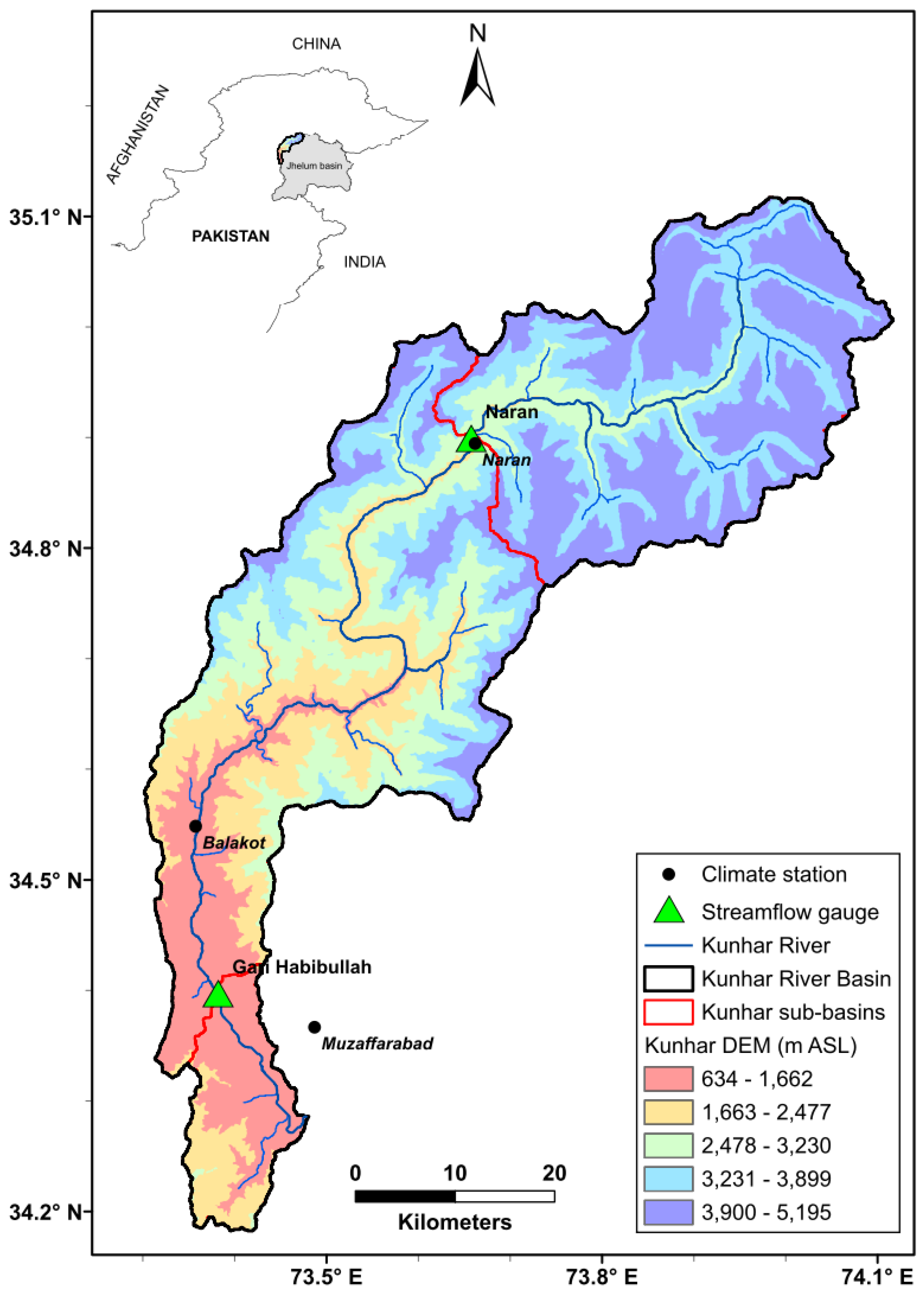
The Kunhar River basin is located in the northern side of Pakistan and stretches between 34.2°–35.1° N and 73.3°–74.1° E, as is shown in Figure 1. The Kunhar drains the southern slope of the Greater Himalayas, located in the Khyber Pakhtunkhwa (KPK) province of Pakistan. It originates from the Lulusar Lake in the Kaghan valley of KPK. It passes through Jalkhand, Bata Kundi, Naran, Kaghan, Kawai, Balakot, and Gari Habibullah and finally joins the Jhelum River at Rara. The Kunhar’s water is rich in algal flora, resulting in a great diversity of the aquatic life it harbors [34]. It has a drainage area of 2535 km², with elevation ranging from 600 to 5000 m (Figure 1).

The Kunhar is one of the biggest tributaries of the transboundary Jhelum River basin. This is the only main tributary which is entirely situated in Pakistan’s territory and therefore, has great importance from the perspective of hydrological monitoring by the WAPDA of Pakistan. The Kunhar contributes about 11% of the total flow to the Mangla Reservoir constructed in the Jhelum River basin. The Mangla Reservoir is the second largest water storage site in the country. The water stored here is primarily used for irrigating 6 million hectares of land in the country and for generating hydropower. The installed capacity of the Mangla power plant is 1000 MW, and electricity is generated as a byproduct [1,35]. Snowmelt from the Kunhar basin contributes about 65% to the total discharge of the Kunhar River and 20%‒40% to the Jhelum River at Manga [35]. The population in the Kunhar basin is almost entirely rural and their economy is generally agro-pastoral based. The principal occupation of the population is agriculture, although rearing livestock is also practiced in the adjacent mountainous areas. A small portion of the population is involved in trade, local labor, and employment in the bigger cities of the country [36]. In Pakistan, 93% of the total annual flow is used for agricultural purposes, 5% for industrial use, and 2% for domestic use [37]. The water of the Kunhar River is mostly used for irrigation, municipal use, power generation, and recreation [35]. Since no industries are located in the basin, most of the water of the Kunhar Basin (about 98%) is used for agriculture and the rest for domestic use.

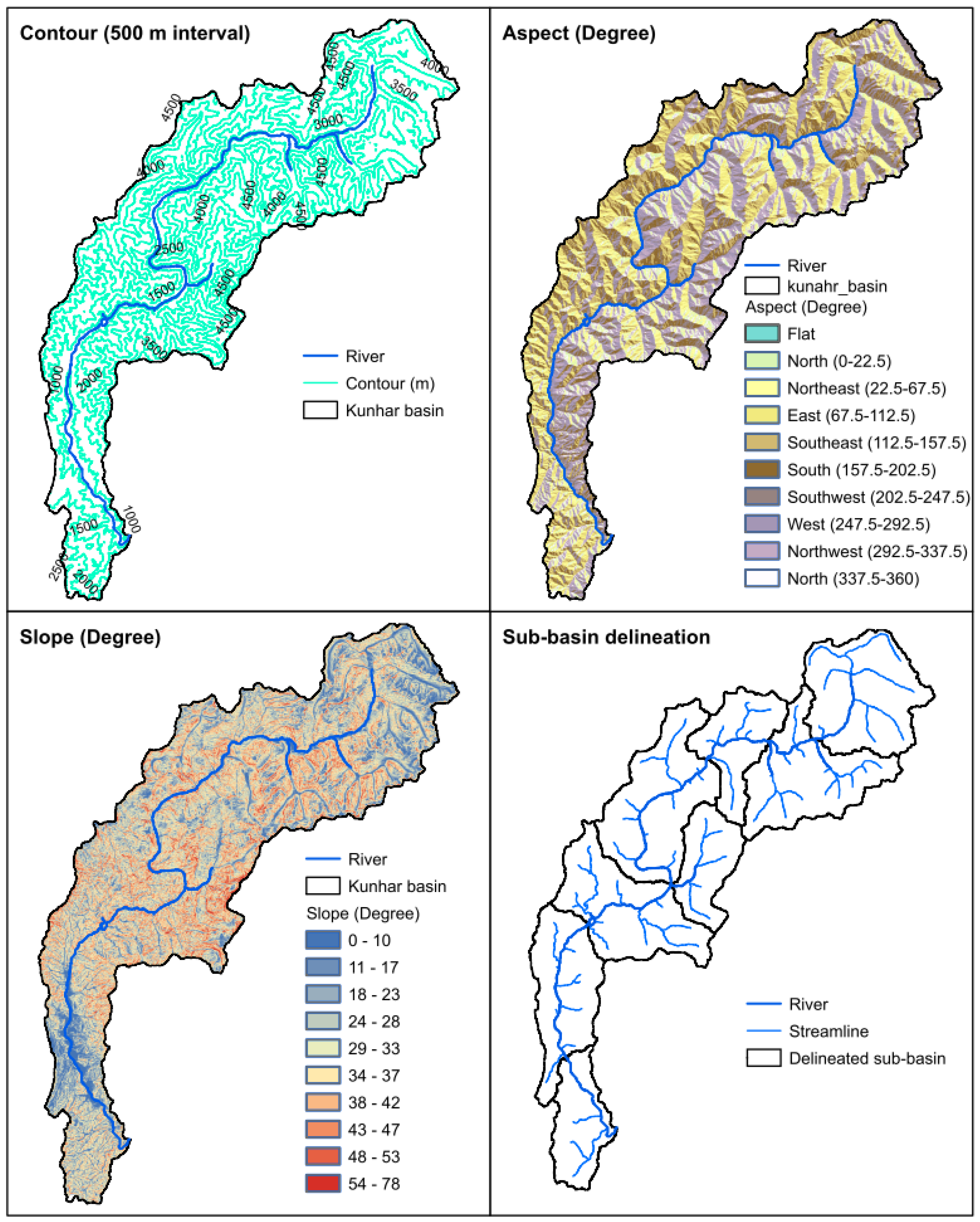
The data of other major topographical characteristics such as slope, contours lines, aspects, and delineated sub-basins, which were extracted from DEM, are presented in Figure 2. This figure shows that the basin has undulating relief ranging from 0° to 78°. The plains along the course of the Kunhar River are located on a gentle slope (0°‒10°). However, most parts of the basin have moderate (>10° and <30°) to steep slopes (>30°).

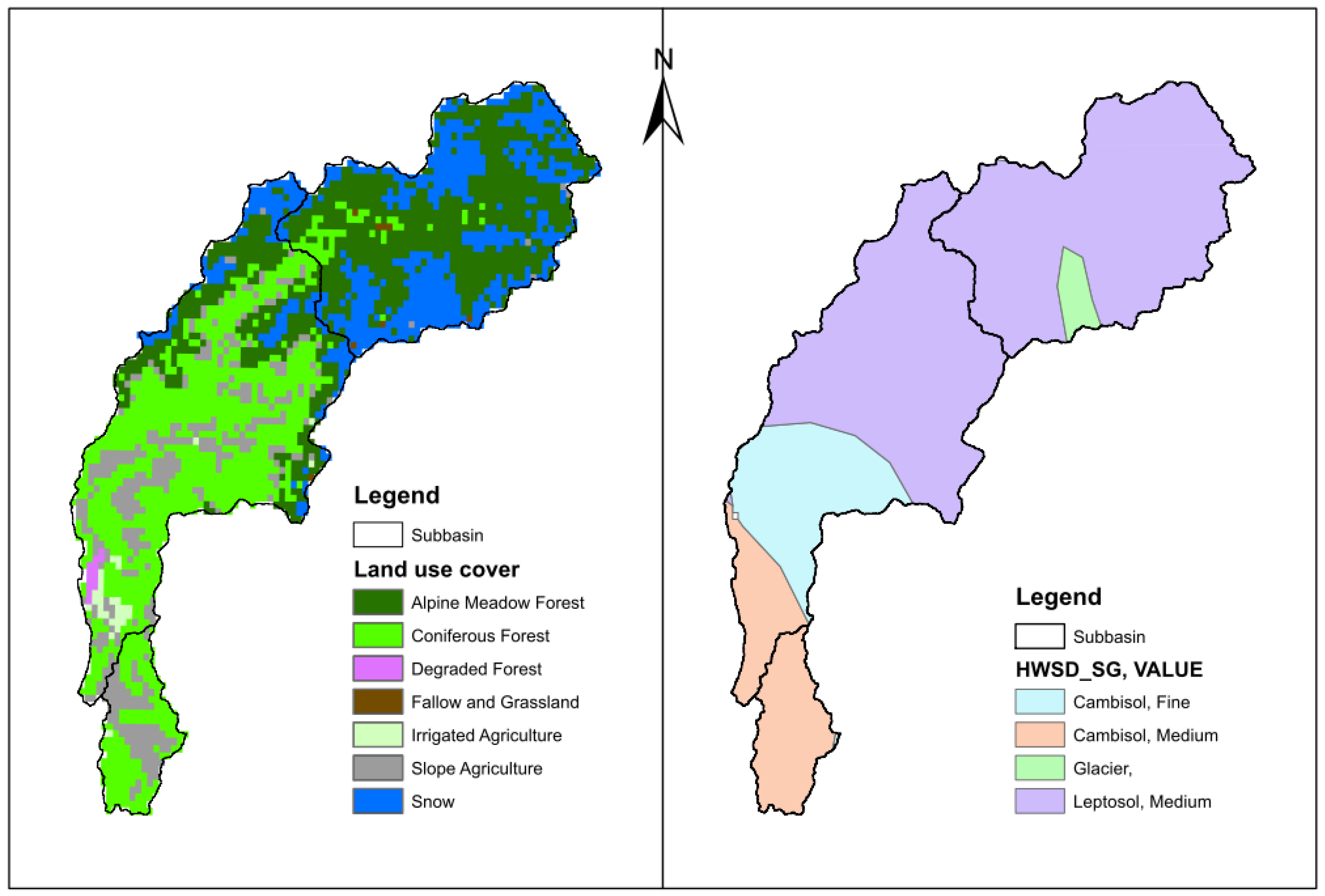
The basin has a great diversity of vegetation such as temperate coniferous forests, subtropical coniferous forests, alpine meadows, agricultural cover, and snow, as described in Table 2 and shown in Figure 3. These varied land covers are reclassified into seven main classes to explore the major land use covers in the basin. Forest, agriculture, and snow cover the maximum area of the basin with about 65%, 14%, and 20% respectively (Table 2). This information was derived from the land cover data of 1 km resolution in the basin.

Table 2. Basic characteristics of soil and land use data in the Kunhar River basin.

	HWSD-Soil Group	Area		Texture	Top Soil Fraction			TSGC
		%	km2		Sand (%)	Silt (%)	Clay (%)	Gravel (%)
1	Cambisol	14	344	Medium	42	36	22	9
2	Cambisol	13	342	Fine	22	30	48	8
3	Leptosol	71	1801	Medium	43	34	23	26
4	Glacier	2	48	-	0	0	0	0
	Land use cover	Area		Land Use Cover
	Re-classes	%	km2	Original
1	Coniferous Forest	33.1	838	Temperate Conifer/Subtropical Conifer/Tropical Moist Deciduous
2	Degraded Forest	0.4	11	Degraded Forest
3	Fallow and Grassland	0.3	7	Slope Grasslands/Sparse vegetation (cold)/Gobi/Desert (cold)
4	Alpine Meadow Forest	31.8	805	Alpine Meadow
5	Irrigated Agriculture	1.0	25	Irrigated Agriculture
6	Slope Agriculture	13.0	329	Slope Agriculture
7	Snow	20.5	521	Snow

HWSD, Harmonized World Soil Database; TSGC, Top Soil Gravel Content.

Table 2. Basic characteristics of soil and land use data in the Kunhar River basin.

	HWSD-Soil Group	Area		Texture	Top Soil Fraction			TSGC
		%	km2		Sand (%)	Silt (%)	Clay (%)	Gravel (%)
1	Cambisol	14	344	Medium	42	36	22	9
2	Cambisol	13	342	Fine	22	30	48	8
3	Leptosol	71	1801	Medium	43	34	23	26
4	Glacier	2	48	-	0	0	0	0
	Land use cover	Area		Land Use Cover
	Re-classes	%	km2	Original
1	Coniferous Forest	33.1	838	Temperate Conifer/Subtropical Conifer/Tropical Moist Deciduous
2	Degraded Forest	0.4	11	Degraded Forest
3	Fallow and Grassland	0.3	7	Slope Grasslands/Sparse vegetation (cold)/Gobi/Desert (cold)
4	Alpine Meadow Forest	31.8	805	Alpine Meadow
5	Irrigated Agriculture	1.0	25	Irrigated Agriculture
6	Slope Agriculture	13.0	329	Slope Agriculture
7	Snow	20.5	521	Snow

HWSD, Harmonized World Soil Database; TSGC, Top Soil Gravel Content.

There are three main groups of soils in the Kunhar River basin, as shown in Figure 3: 1) cambisol fine, 2) cambisol medium, and 3) leptosol. Cambisol characterizes weak to moderately developed soils and it (both fine and medium varieties) covers 27% of the basin, while leptosol is very shallow soil over hard rock and is unconsolidated and very gravelly material. Leptosol covers around 71% area of the basin. Some glacier patches also exist in the upper part of the basin. The basic information about soil types found in the basin is given in Table 2. The properties of these soils were derived from the soil data of 1 km resolution in the basin.

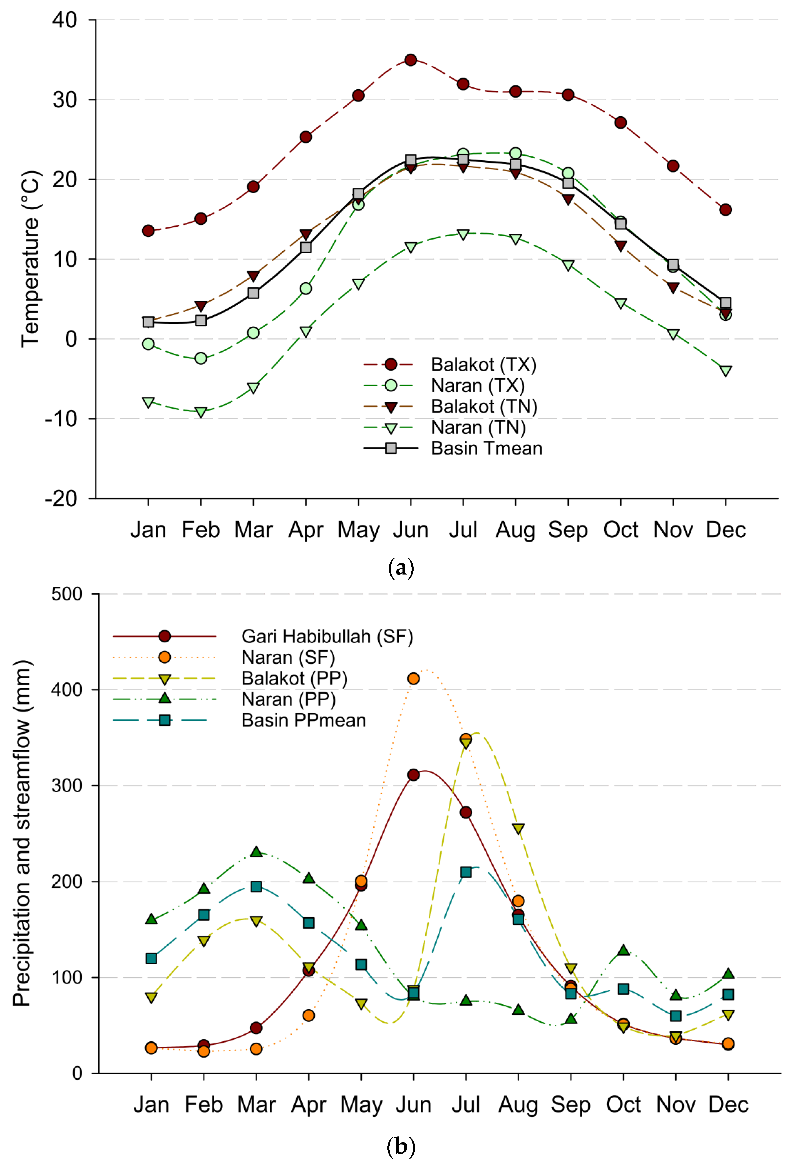
The Kunhar basin is located in a humid, subtropical zone. In the present study, hydro-climatic data was processed for the period of 1961–2000 to extract some basic information about the hydro-climatic conditions in the basin. This information is presented in Figure 4. The average annual temperature in the basin is about 13 °C (2 °C–23 °C). February is the coldest and July is the warmest month here. This was calculated from the data of the Naran and Balakot climate stations available for the period of 1961‒2000. At Balakot, located in the lower part of basin (Figure 1), TN ranges from 2 °C (January) to 23 °C (July) and TX from 14 °C (January) to 35 °C (June). At Naran, located in the upper part of the basin, TN ranges from −9 °C (February) to 13 °C (July) and TX from −1 °C (February) to 23 °C (July) (Figure 4a). The Kunhar basin has an annual precipitation of about 1500 mm (Table 1) with two peaks (Figure 4b). The first peak occurs in the upper part of the basin in the month of March because of the Western Disturbances (WDs) system in winter. Most parts of Pakistan, and its northwestern parts primarily, obtain precipitation due to WDs. WDs are caused by depressions over Mediterranean regions, resulting in precipitation over central and southwest Asia in the months of December to March [38,39]. The second peak happens in the month of July and in the lower parts of the basin due to the summer monsoons, which are the result of the saturated south western winds from the Bay of Bengal and Arabian Sea. It can be concluded that the monsoons do not reach the upper part of the basin, although WDs affect the whole basin. On the other hand, there is only one big streamflow peak, both in the upper (Naran) and lower parts (Gari Habibullah) of the basin, that occurs in the month of July (Figure 4b). This means the precipitation from December to March (winter) accumulates as snow cover, especially in the upper parts of the basin, and then starts melting after March and lasts till July when it overlaps with monsoon precipitation and results in one big peak. An average flow of about 1350 mm (103 m³/s) has been measured at Gari Habibullah near the mouth of the basin for the period of 1961‒2000. The same was reported by de-Scally as well [39].

Figure 4. Monthly (a) max temperature (TX), min temperature (TN), (b) precipitation (PP), and streamflow (SF) in the Kunhar River basin for the period of 1961–2000.

Figure 4. Monthly (a) max temperature (TX), min temperature (TN), (b) precipitation (PP), and streamflow (SF) in the Kunhar River basin for the period of 1961–2000.

4. Methodology

4.1. Description of HEC-HMS

The Hydrological Modeling system (HEC-HMS) is a rainfall-runoff simulation software used for a wide range of watersheds from large river basins to small urban areas. The model was formulated by the U.S. Army Corps of Engineers at the Hydrologic Engineering Center (HEC). HEC-HMS comprises different loss techniques such as SCS curve number, initial and constant, Green Ampt, one-layer deficit-constant, Smith Parlange, and five-layer soil moisture accounting. These techniques are used to estimate excess precipitation in fairly simple to very complex infiltration and evapotranspiration environments. This model can be used for both event and continuous modeling.

In order to calculate direct runoff from excess precipitation, seven methods including SCS, Clark, Snyder, and ModClark are available in the system. This model also consists of five base flow methods including recession method, constant monthly method, and linear reservoir method, and six channel routing methods including Muskingum, and modified pulse methods. It also has six kinds of meteorological models like Thiessen and inverse distance methods to analyze meteorological data such as precipitation, evapotranspiration, and snowmelt. The meteorological model extracts the precipitation for each sub-basin in the watershed. However, currently, only two methods (Temperature Index and Gridded Temperature Index) are available to compute runoff from snowfall in this modeling system [40,41].

A complete basin model setup for rainfall-runoff processes comprises a basin model, a meteorological model, control specification, and input time series. The basin model describes the physical characteristics of the study region such as the areas of sub-basins and river lengths of a watershed. Each basin model in HEC-HMS consists of a loss method, a transforming method, a base flow method, and a channel routing method [23]. Control specification is one of the main components of this model’s setup and it controls the simulation period. For example, it controls when the model is to start and stop, and what the time interval for simulation should be. The input time series encompasses precipitation, temperature, evapotranspiration, and observed streamflow etc., which have a direct link with the basin’s model and the meteorological model. A detailed description of the model’s formulation and its various processes is provided in the User’s Manual and Technical Reference Manual of HEC-HMS [40] (p. 318 and p.157).

In the present study, the basin model was developed using the deficit and constant loss (DCL) method for calculating excess precipitation, the SCS unit hydrograph for transforming direct runoff, Muskingum for channel routing, and the recession method for base flow. The meteorological model was established using the Thiessen polygon gauge weight method for precipitation calculation, the temperature index method for snowmelt modeling, and the monthly evapotranspiration method. The Thiessen polygons were created and their weights were calculated by HEC-GeoHMs in accordance with the precipitation gauges. The same combination has been used in different studies [15,17,18].

The DCL model computes excess precipitation in a watershed. It is a single layer continuous method used for calculating the changes in soil moisture content. It is similar to the initial and constant loss (ICL) method but this method recovers the initial losses after a long period of no precipitation. This method contains four main parameters: maximum deficit, initial deficit, constant rate, and impervious percentage. These parameters can be initially estimated using soil and land cover data as initial inputs for the model but are finalized only during the calibration process.

The excess precipitation calculated from DCL was transformed into direct surface runoff by the SCS unit hydrograph method. Basin lag is the only parameter of the SCS method, and it needs to be determined during calibration. It can also be estimated as an initial value for calibration by multiplying the time of concentration by 0.6. In this study, the recession method was used to calculate the base flow which contributes to the total flow from the watershed. Three parameters—initial discharge, recession constant, and threshold—were determined during calibration.

To transfer the total flow from one point to other, the Muskingum method was used. This method is a simple mass conservation scheme for routing flow through channels. There are two main parameters for this method: travel time (K), and the Muskingum coefficient (X). The Muskingum coefficient ranges between 0 and 0.5.

The Thiessen polygon method was used to assign weights to each gauge in the watershed during the development of the meteorological model. For snowmelt modeling, different elevation bands were used for each sub-basin in the temperature index method (TIM). TIM is an extension of the degree-day technique to calculate flow from snowpack. In the degree-day approach, a fixed amount of snowmelt is assigned for each degree above freezing point. This method is a conceptual representation of the cold energy stored in the snowpack. This also takes care of past conditions and some other climatic factors during the calculation of snowmelt. Different parameters such as base temperature, wet melt rate, rain rate limit, melt rate pattern, lapse rate, and antecedent temperature index are required for this method [32]. A lapse rate of −7.0 °/km was calculated for the study area and kept constant for the entire Kunhar River basin. 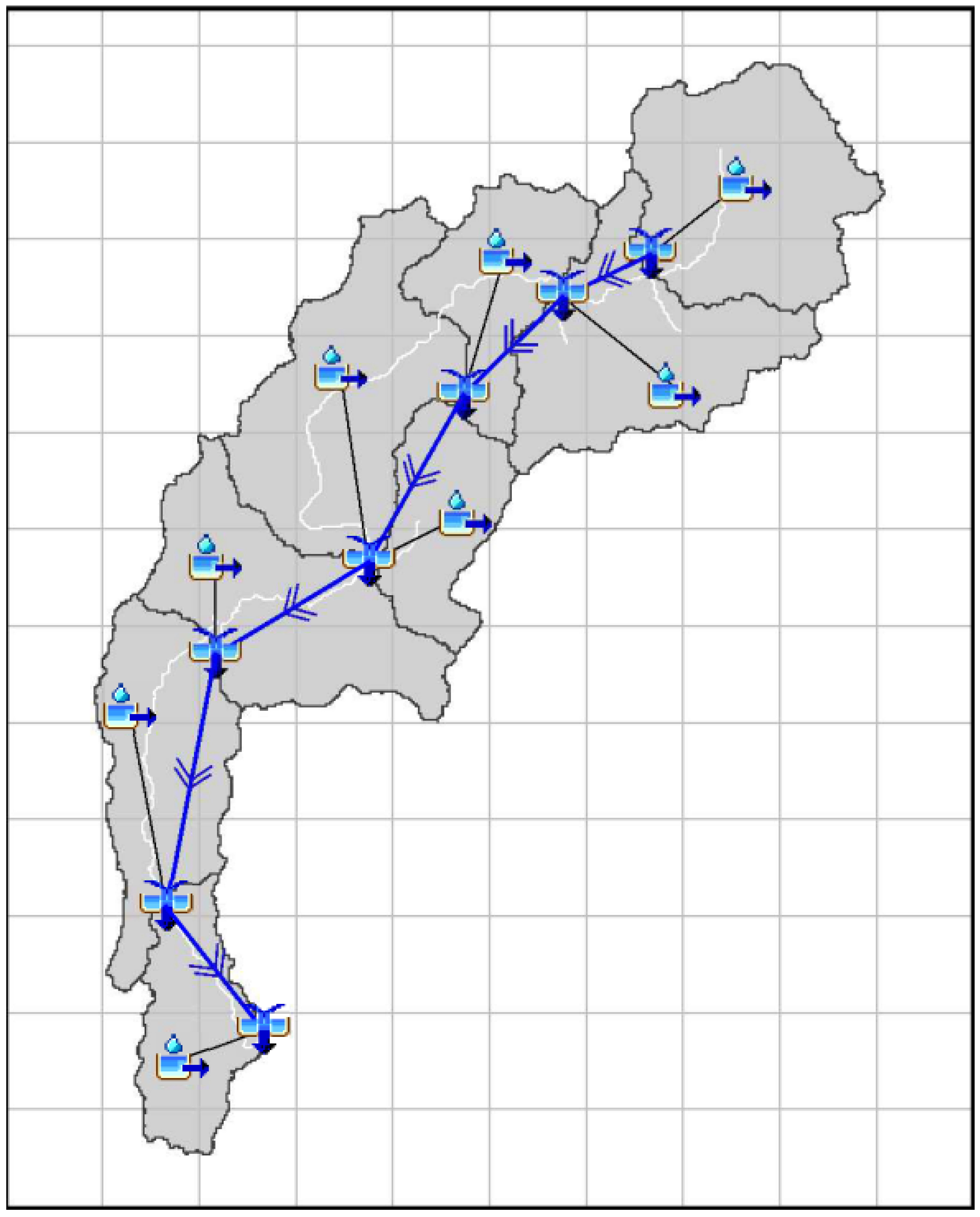The FAO Penman-Monteith method—recommended as the standard method for computing potential evapotranspiration [24]—was carried out to calculate the potential evapotranspiration in the basin. A schemetic diagram for the setup of HEC-HMS in the Kunhar River basin is shown in Figure 5.

Figure 5. Schemetic diagram for the setup of HEC-HMS hydrological modeling system.

Figure 5. Schemetic diagram for the setup of HEC-HMS hydrological modeling system.

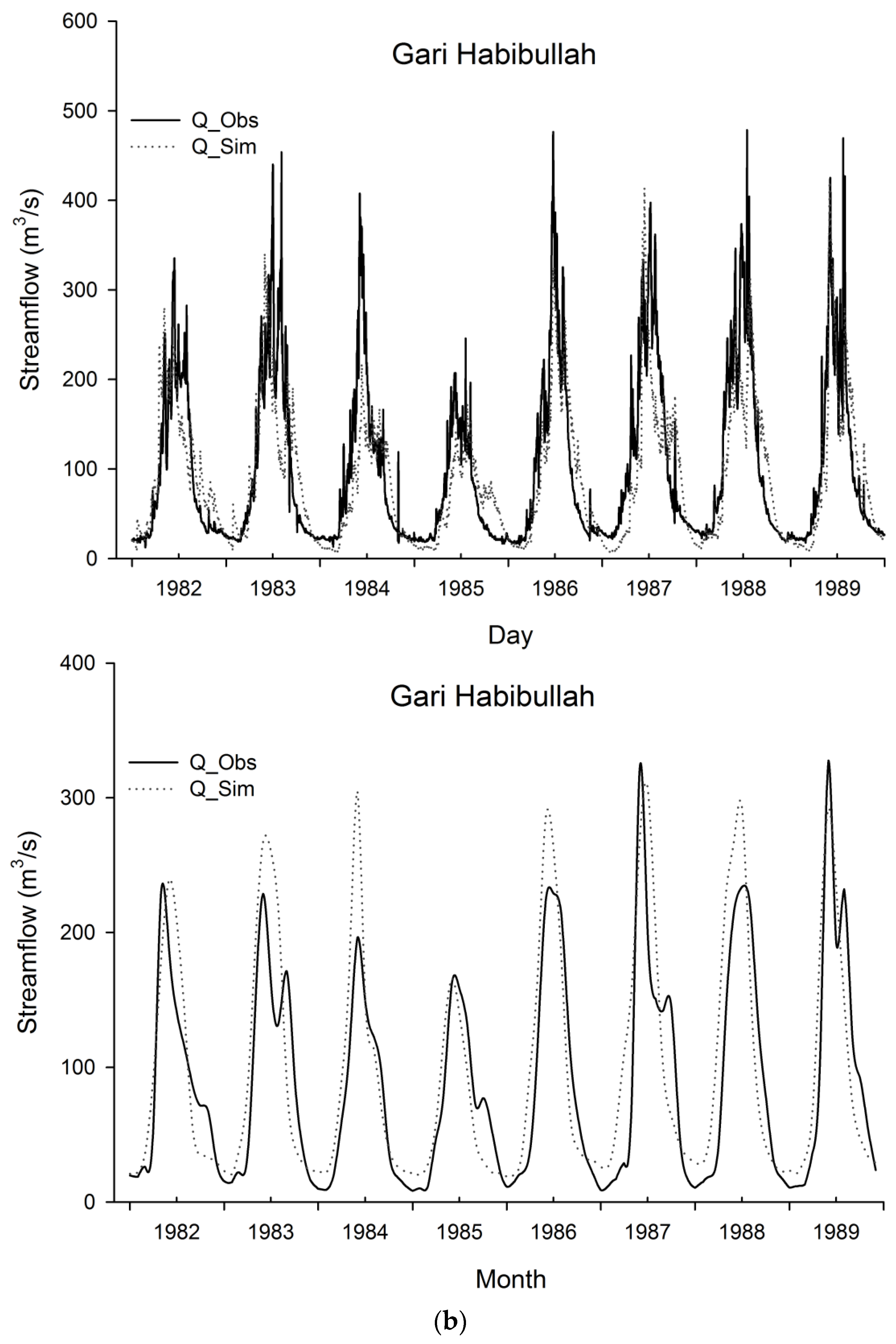
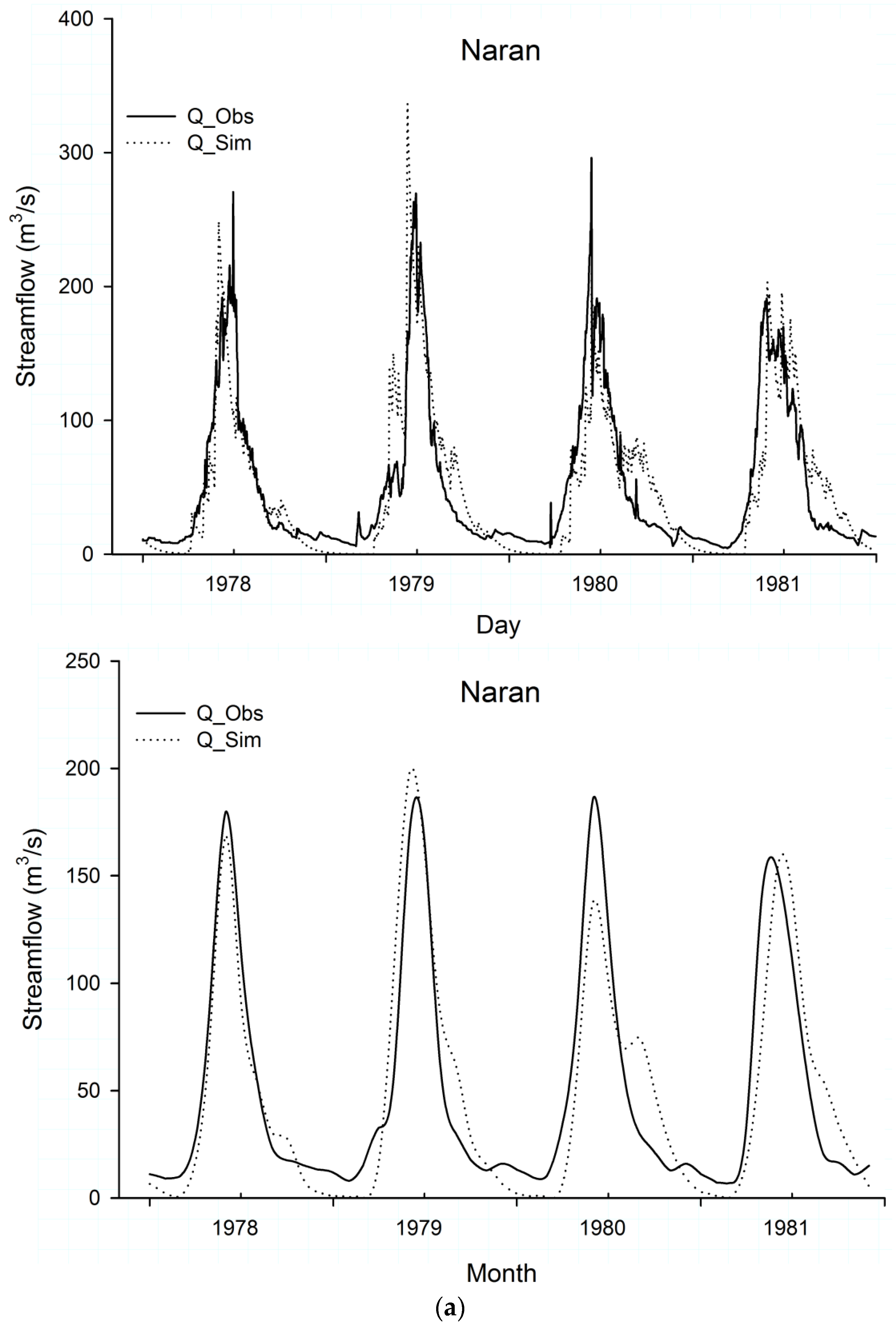
4.2. The Model’s Calibration and Validation

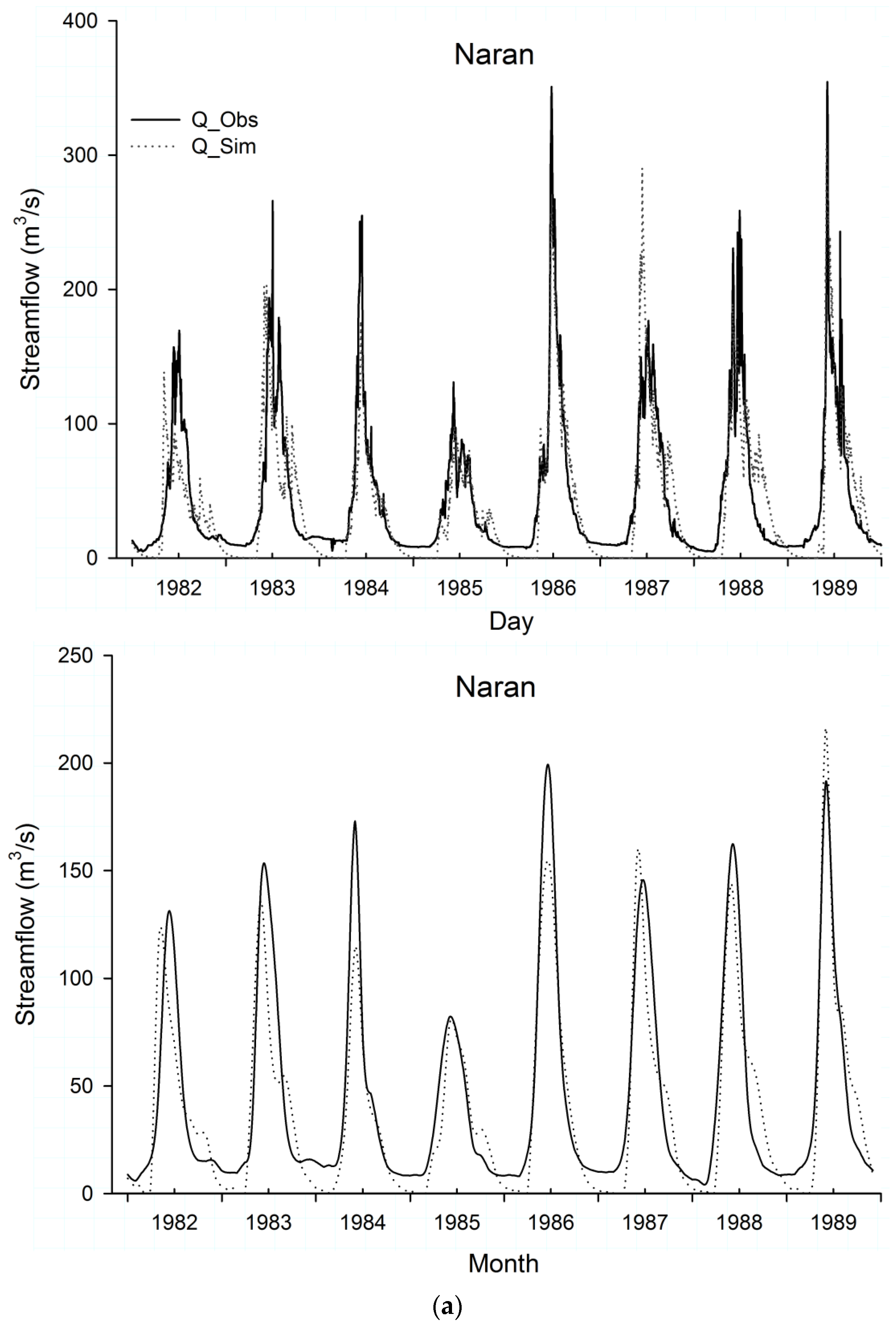
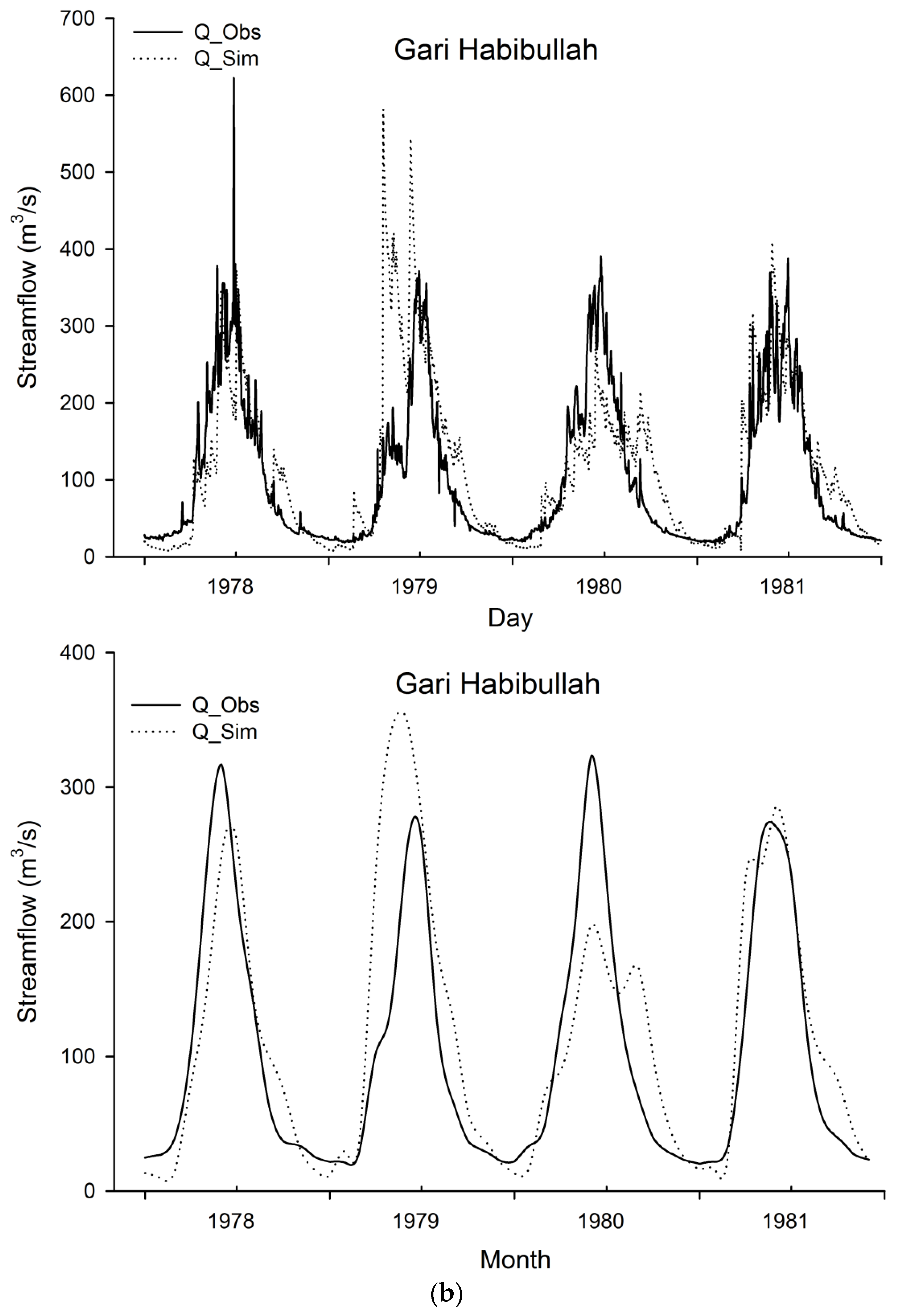
The calibration of a model is a process in which the model’s parameters are adjusted in such a way that the simulated flow captures the variations of the observed flow [25]. In this study, a split sample method was used for calibration and validation. In this method, the calibration period does not overlap with the validation period. A data period of eight years, from 1982 to 1989, was chosen as the calibration period and the period from 1978 to 1981 for validation because these periods had minimum missing values of both precipitation and streamflow. The physical properties—land use cover and soil properties—of the watershed were considered as constant during the simulation period.

Nelder Mead and Univariate Gradient are the two main algorithms to optimize the objective function. There are seven different kinds of objective functions in HEC-HMS. In this study, the sum of the squared residual was chosen and was minimized using the Nelder-Mead algorithm to explore the optimized model parameters in order to get the best results of the simulation. The simulated flows were compared with the observed flow using the coefficient of determination (R²), percent deviation (D), and Nash-Sutcliffe efficiency (E). The R² values indicate how well the variations in the observed data are captured by the simulated data, D describes the mean percent deviation between observed and simulated flow, and E shows how well the observed plot fits with the simulated plot [22]. For more illustrative purposes, the simulated data was also compared with observed data graphically to explore how well the low and high observed flows were captured by simulated flow. In the present study, the model was calibrated and validated at both Naran and Gari Habibullah gauging stations.

The model’s performance parameters—R², D, and E—were calculated using the following equations:

$$R^2=\frac{{{\displaystyle \sum }}^{\text{}}\left(Q_{obs}-\overline{Q_{obs}}\right)\times \left(Q_{sim}-\overline{Q_{sim}}\right)}{\sqrt{{{\displaystyle \sum }}^{\text{}}{\left(Q_{obs}-\overline{Q_{obs}}\right)}^2\times {\left(Q_{sim}-\overline{Q_{sim}}\right)}^2}}$$

(1)

Q_obs and Q_sim are observed and simulated values respectively. If the value of R² is close to 1, it indicates a good correlation between simulated and observed flows. The correlation is considered optimum if R² is exactly equal to 1 [22].

$$D(\%)=100\times \frac{{{\displaystyle \sum }}^{\text{}}\left(Q_{sim}-Q_{obs}\right)}{{{\displaystyle \sum }}^{\text{}}{Q}_{obs}}$$

(2)

The value of D should ideally be close to 0%. Positive and negative values are respectively indicators of over- and under-estimation by the model [22].

$$E=1-\frac{{{\displaystyle \sum }}^{\text{}}{\left(Q_{sim}-Q_{obs}\right)}^2}{{{\displaystyle \sum }}^{\text{}}{\left(Q_{obs}-\overline{Q_{obs}}\right)}^2}$$

(3)

The value of E lies between 0 and 1. A positive value close to 1 implies good calibration while a negative value close to 0 is not acceptable. If the value of E is greater than 0.75, then the results are considered to be good, and if it is between 0.36 and 0.75, the results are satisfactory [41].

4.3. Projected Changes in Streamflow

After successful calibration and validation, the downscaled daily time series (A2 and B2) of precipitation and temperature for the period of 2011 to 2099 were used as input for HEC-HMS to simulate daily flow data at both gauges (Naran and Gari Habibullah). The physical characteristics of the Jhelum basin were kept constant throughout the simulation period. However, it cannot be ignored that these characteristics do vary with time. The simulated data were divided into three periods: the 2020s (2011–2040), the 2050s (2041–2070), and the 2080s (2071–2099) and all three were compared with the baseline period (1961–1990) to assess changes in flow in the future. Different indicators such as mean flow, low flow, median flow, high flow, flow duration curves, temporal shift in peaks, and temporal shifts in center-of-volume dates were calculated for the three periods and the results were compared to the baseline period’s data so as to explore the impact of climate change on the streamflow in the basin.

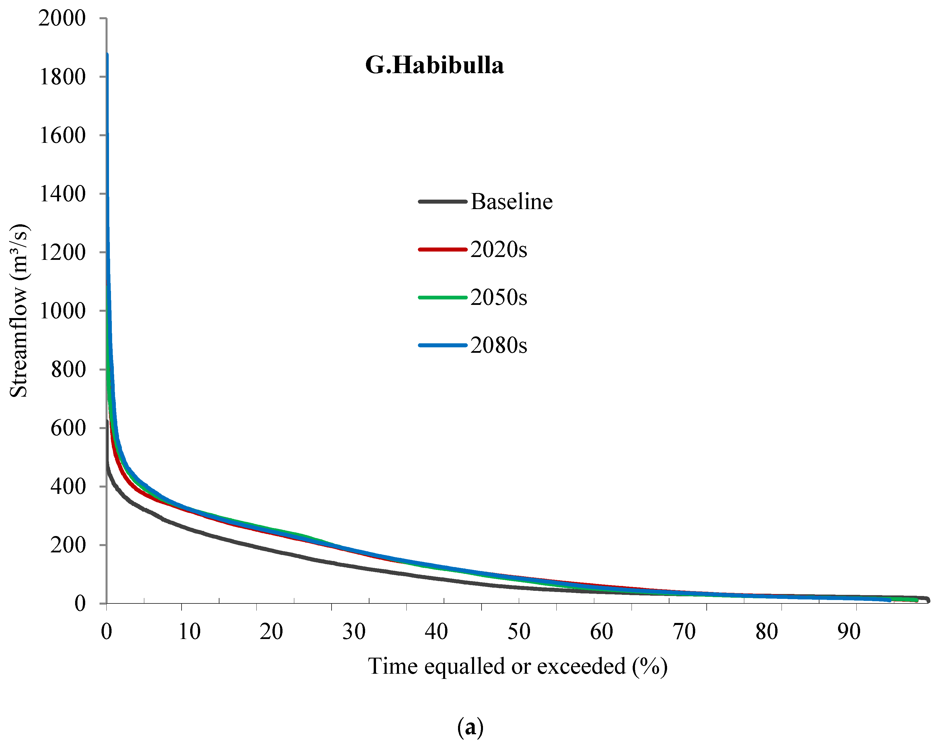
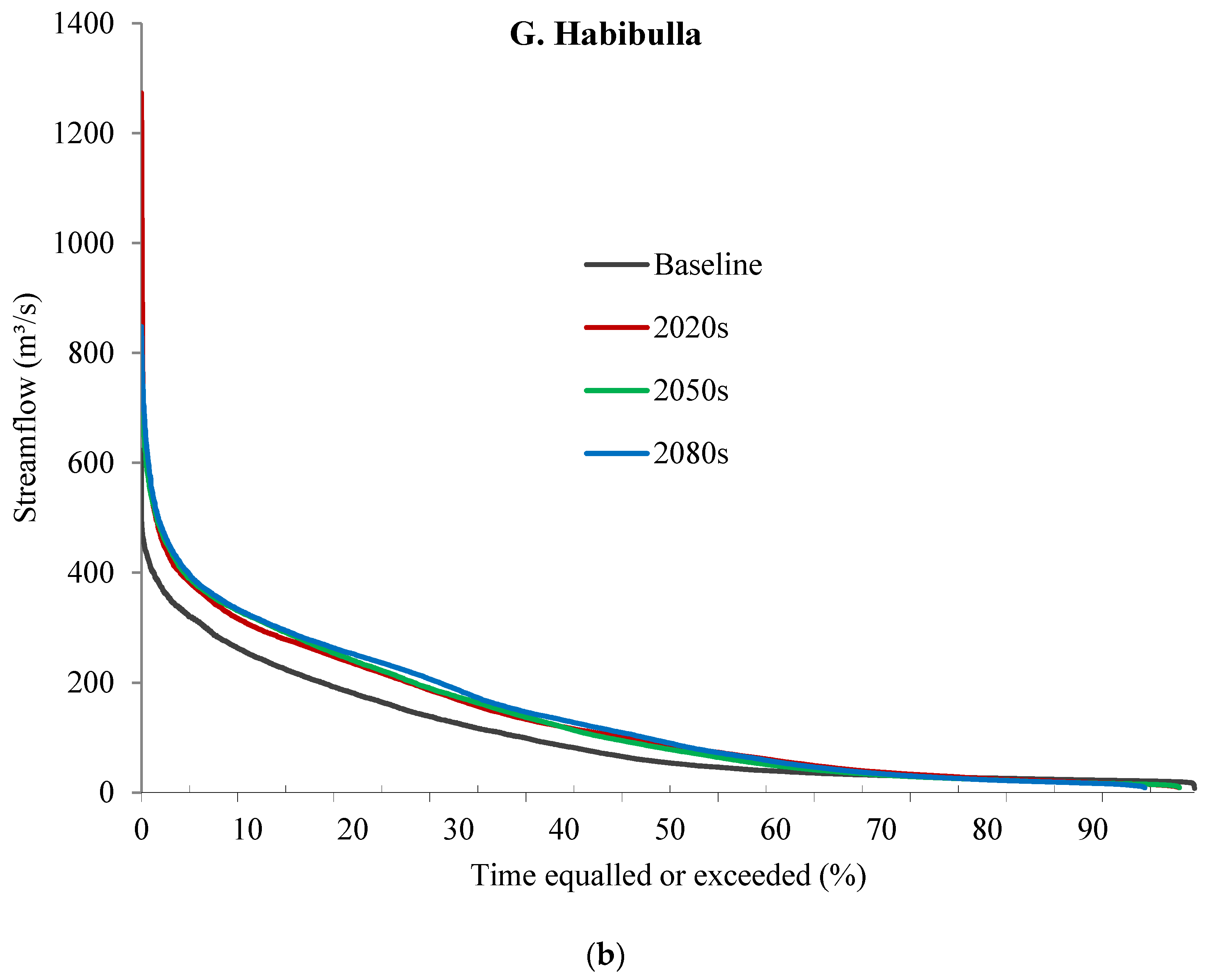
When analyzing streamflow to construct an installation such as a reservoir and headwork on a river, two questions are frequently asked: (1) how often will the streamflow occur in the future? and (2) what will be the magnitude of the streamflow? Flow duration curves are the main tools to deal with these two questions. These curves present the percentage of times that the flow in a stream is likely to exceed or be equal to a specified value of the flow. These curves can be applied in different kinds of studies such as hydropower management, reservoir sedimentation, water quality management, and low and high flow studies [42]. The following equation is used to construct the flow duration curves:

$$P(\%)=\frac{M}{\left(n+1\right)}\times 100$$

(4)

P or the probability of flow is equal to or exceeds a specified value (% of time), M is the rank of events, and N is the number of events in a specified period of time.

In the present study, the daily time series were used to construct the flow duration curves for the base period (1961–1990) and for the three future periods: the 2020s, 2050s, and 2080s.

5. Results and Discussion

5.1. Calibration and Validation

Table 3 shows the model’s performance parameters (E, D, and R²) that were calculated using the daily and monthly observed and simulated streamflows for calibration (1982–1989) and validation (1978–1981) at Naran and Gari Habibullah. In the case of daily data, the values of E and R² ranged from 0.55 to 0.74 during calibration and validation at both stations, and the D values lay between −9% and 12%. The D values show that the model underestimated values during the calibration and validation periods at Naran and also underestimated them at Gari Habibullah during calibration. However, the model overestimated the values during validation at the Gari Habibullah station. The results were greatly improved when these parameters were calculated from the monthly time series. The values of E and R² were improved to 0.63–0.88. These results are quite satisfactory and complement well some previous studies such as Meenu et al. [22] in India, Verma et al. [23] in India, Yimer et al. [24] in Ethiopia, and Garcia et al. [25] in Spain. All these studies also used HEC-HMS to simulate streamflow for climate change studies, with E ranging from 0.48–0.83 and R² from 0.63–0.84.

Table 3. Nash-Sutcliffe efficiency (E), coefficient of determination (R²), and percent deviation (D) for calibration (1982–1989) and validation (1978–1981) for different stream gauges, calculated from daily and monthly data, in the Kunhar River basin.

Hydrometric Station	Calibration			Validation
	E	R2	D (%)	E	R2	D (%)
From daily streamflow
Naran	0.71	0.74	−7.78	0.71	0.73	−3.13
Gari Habibullah	0.66	0.67	−8.69	0.55	0.65	12.17
From monthly streamflow
Naran	0.83	0.84	−11.02	0.83	0.84	−3.14
Gari Habibullah	0.88	0.85	−9.92	0.63	0.70	12.18

Table 3. Nash-Sutcliffe efficiency (E), coefficient of determination (R²), and percent deviation (D) for calibration (1982–1989) and validation (1978–1981) for different stream gauges, calculated from daily and monthly data, in the Kunhar River basin.

Hydrometric Station	Calibration			Validation
	E	R2	D (%)	E	R2	D (%)
From daily streamflow
Naran	0.71	0.74	−7.78	0.71	0.73	−3.13
Gari Habibullah	0.66	0.67	−8.69	0.55	0.65	12.17
From monthly streamflow
Naran	0.83	0.84	−11.02	0.83	0.84	−3.14
Gari Habibullah	0.88	0.85	−9.92	0.63	0.70	12.18

The graphical comparisons of observed against simulated flow for the calibration and validation periods are shown in Figure 6 and Figure 7 respectively. At both Naran and Gari Habibullah gauging stations, patterns of observed flow were well matched by patterns of simulated flow during the calibration period. However, the peak and low flows were not captured well by the model. At Naran, in some years, peak and low flows were underestimated by the model but it was the reverse in the case of Gari Habibullah. This underestimation of flow might be due to the lack of enough precipitation gauges available in the basin or it might be due to the use of a simple temperature index model to calculate flow from snowmelt because about 65% of the total flow comes from snowmelt. Over- and under-estimation of flow must be considered during the discussion of this study’s results. For example, at Gari Habibullah, the model overestimated the flow by 12%. This means that if the projected increase at Gari Habibullah is 50%, then the final projected increase will be 38%.

In the case of validation, the peaks were comparatively better captured by the simulated flow at both stations, especially at Naran. On the whole, the calibration and validation results were satisfactory and comparable with some previous studies like Meenu et al. [22], Verma et al. [23], Yimer et al. [24], and Garcia et al. [25].

The present study’s results could be much more exact if the number of precipitation gauges were more than are currently available. In the present study, the vegetation cover (where 20% is snow cover) was considered constant for the entire calibration and validation periods. Vegetation cover, especially snow cover, could not have been the same for all the years of the calibration and validation periods. It can be concluded that taking into consideration changes in vegetation cover will perhaps improve the results.

Figure 6. Comparison of daily and monthly observed and simulated streamflow at (a) Naran and (b) Gari Habibullah for calibration (1982‒1989) in the Kunhar River basin.

Figure 6. Comparison of daily and monthly observed and simulated streamflow at (a) Naran and (b) Gari Habibullah for calibration (1982‒1989) in the Kunhar River basin.

Figure 7. Comparison of daily and monthly observed and simulated streamflow at (a) Naran and (b) Gari Habibullah for validation (1978‒1981) in the Kunhar River basin.

Figure 7. Comparison of daily and monthly observed and simulated streamflow at (a) Naran and (b) Gari Habibullah for validation (1978‒1981) in the Kunhar River basin.

5.2. Projected Changes in Mean Streamflow

Table 4 outlines, in percentage, the projected changes in seasonal and annual flows in the 2020s, 2050s, and 2080s with respect to the baseline period (1961–1990) under A2 and B2 scenarios. In all three periods and under both scenarios, the flow in winter (DJF) and spring (MAM) seasons was projected to decrease at both gauges except in winter at Gari Habibullah in the 2080s. In both seasons, the negative changes at Naran (ranging from 40%‒73%) were greatly higher than Gari Habibullah, (ranging from 6% to 28%) under both A2 and B2. Mahmood and Babel [43] conducted a study about extreme temperature events in the Jhelum River basin under A2 and B2, and they found that the intensity of cold days and cold nights will increase in the future. The reduction in flow (as indicated by the results of this study) is likely to be the case due to more accumulation of snowfall that would result from the increased intensity of cold days and cold nights in winter (based on the projections of Mahmood and Babel that indicate that precipitation will increase in winter and decrease in spring) [1].

Conversely, the summer (JJA) and autumn (SON) seasons were projected to have increased flow in all three future periods and under both scenarios but with different magnitudes. Autumn showed highest projected increase at both stations and under both scenarios, ranging from 91% to 131%. This high increase in autumn flow is most likely due to the most projected increase of 25%‒32% in precipitation indicated by Mahmood and Babel [1]. The projected changes in this study appear much more than the projected changes in precipitation explored by Mahmood and Babel [1]. This could be because the vegetation cover was considered to be constant throughout the simulation period in this study. In the present state, snow cover (20%) dominates the basin and we used the same percentage of snow cover and constant proportions of other vegetation types for the simulation of projected flow. It is quite possible that snow cover will reduce in the future because of increasing temperature in the basin. So, along with validation results wherein the model overestimated by about 12%, if we also reduce snow cover, then the changes would be less than the projected changes.

On the whole, the mean annual flow was projected to increase by 42%–43% at the end of this century in the basin (at both sites) under both scenarios. The high increase in flow in summer and autumn and the decrease in winter and spring shows that it is hard to rely on only one GCM. So, a group of GCMs is required to give a clearer picture about these results.

The projected decrease in winter and spring can cause water shortage during these seasons not only for the agriculture sector but also for the domestic sector. On the other hand, the projected increase in summer (monsoon season) and autumn can result in flooding in the basin, and that can cause economic losses in the basin. These losses can be reduced by building reservoirs in the basin which can be used to store water during the flooding season and the stored water can be used during the period of shortage.

Table 4. Future changes (%) in streamflow at different gauges relative to the baseline period (1961‒1990) under A2 and B2 scenarios in the Kunhar River basin.

A2 Scenario	1961–1990 (m3/s)		2020s		2050s		2080s
	Naran	G. Habib	Naran	G. Habib	Naran	G. Habib	Naran	G. Habib
Winter	10	25	−70	0	−71	−6	−70	8
Spring	37	110	−56	−14	−52	−26	−40	−12
Summer	121	226	53	38	51	46	61	49
Autumn	24	58	104	109	98	107	111	126
Annual	48	105	8	33	6	30	16	43
B2 Scenario
Winter	10	25	−73	−2	−73	−11	−70	2
Spring	37	110	−62	−16	−58	−28	−49	−10
Summer	121	226	58	38	56	43	54	46
Autumn	24	58	88	97	92	91	97	131
Annual	48	105	3	29	5	24	8	42

Table 4. Future changes (%) in streamflow at different gauges relative to the baseline period (1961‒1990) under A2 and B2 scenarios in the Kunhar River basin.

A2 Scenario	1961–1990 (m3/s)		2020s		2050s		2080s
	Naran	G. Habib	Naran	G. Habib	Naran	G. Habib	Naran	G. Habib
Winter	10	25	−70	0	−71	−6	−70	8
Spring	37	110	−56	−14	−52	−26	−40	−12
Summer	121	226	53	38	51	46	61	49
Autumn	24	58	104	109	98	107	111	126
Annual	48	105	8	33	6	30	16	43
B2 Scenario
Winter	10	25	−73	−2	−73	−11	−70	2
Spring	37	110	−62	−16	−58	−28	−49	−10
Summer	121	226	58	38	56	43	54	46
Autumn	24	58	88	97	92	91	97	131
Annual	48	105	3	29	5	24	8	42

5.3. Changes in Flow Duration Curve as Well as Low, Medium, and High Flows

Figure 8 displays the comparison of flow duration curves during the baseline period (1961–1990) and the three future periods (2020s, 2050s and 2080s) under A2 and B2 scenarios at the Gari Habibullah hydrometric station. This comparison shows that the probability of occurrence of flow and magnitudes of flow could be higher in the future in the Kunhar basin under both scenarios. Table 5 shows the projected changes in high flow (Q₅), median flow (Q₅₀), and low flow (Q₉₅) in the 2020s, 2050s, and 2080s with respect to the baseline under both scenarios. Under both scenarios, Q₅ and Q₅₀ were projected to increase in all three future periods in the Kunhar basin, with 17%–52% (Q₅) and 43%–84% (Q₅₀). This increase in mean flow is most likely due to the increase in mean annual precipitation and increase in high flow is most likely due to the increase in summer precipitation (monsoon season), as also projected by Mahmood and Babel [1]. However, Q₉₅ was predicted to decrease by 18%–99% in the future in the basin. This might be due to the increase in the intensity of cold days and cold nights (mentioned by Mahmood and Babel [43]) which may cause precipitation as snow accumulation in winter (low flow season).

These changes in high flow and flow duration curve show that the frequency of floods and their magnitudes will increase in the future which will create a lot of management problems in the basin. Flooding can not only cause economic losses but also loss of life. Nonetheless, with proper utilization and management of the increased flow, Pakistan can actually increase food and hydropower production in the basin.

Figure 8. Flow duration curves under (a) A2 and (b) B2 scenarios at Gari Habibullah in the Kunhar River basin.

Figure 8. Flow duration curves under (a) A2 and (b) B2 scenarios at Gari Habibullah in the Kunhar River basin.

Table 5. Percent future changes in low, median, and high flows with respect to the baseline (1961–1990) under A2 and B2 scenarios in the Kunhar River basin.

A2 Scenario	1961–1990 (m³/s)		2020s		2050s		2080s
	Naran	G. Habib	Naran	G. Habib	Naran	G. Habib	Naran	G. Habib
Q5	170	316	41	17	39	22	52	28
Q50	19	54	43	67	44	55	61	76
Q95	8	21	–99	–25	–99	–22	–99	–18
B2 Scenario
Q5	170	316	42	19	46	21	43	24
Q50	19	54	31	65	43	51	45	86
Q95	8	21	–99	–23	–99	–25	–99	–21

Q₅, high flow; Q₅₀, median flow; Q₉₅, low flow.

Table 5. Percent future changes in low, median, and high flows with respect to the baseline (1961–1990) under A2 and B2 scenarios in the Kunhar River basin.

A2 Scenario	1961–1990 (m³/s)		2020s		2050s		2080s
	Naran	G. Habib	Naran	G. Habib	Naran	G. Habib	Naran	G. Habib
Q5	170	316	41	17	39	22	52	28
Q50	19	54	43	67	44	55	61	76
Q95	8	21	–99	–25	–99	–22	–99	–18
B2 Scenario
Q5	170	316	42	19	46	21	43	24
Q50	19	54	31	65	43	51	45	86
Q95	8	21	–99	–23	–99	–25	–99	–21

Q₅, high flow; Q₅₀, median flow; Q₉₅, low flow.

5.4. Temporal Shifts in Peak Flows

In Figure 9, the mean monthly discharge of the baseline period (1961–1990) is plotted against the mean monthly discharge in the future periods (2020s, 2050s, and 2080s) to explore temporal shifts and magnitudes of peak flows at Gari Habibullah. At this site, a definite delay and increase in peak flows were projected in all three future periods under both scenarios. The peak flows were projected to shift from June to July, with about a 10%–25% increase under both scenarios. This shows that the basin will not only face an increase in frequency and magnitude of floods (mentioned in previous sections) but will also face the shift of these floods from June to July.

Figure 9. Future shift of peak flows in timing and magnitude under A2 and B2 in the Kunhar River basin.

Figure 9. Future shift of peak flows in timing and magnitude under A2 and B2 in the Kunhar River basin.

5.5. Temporal Shifts in Center-of-Volume Date (CVD)

To determine the impact of climate change on the timing of streamflows, an indicator such as center-of-volume date (CVD)—a date at which half of the total volume of streamflow passes through at a gauging station for a specific time period—was used in the present study. CVD was calculated according to the equation described in [44]. Table 6 shows the changes in CVD under A2 and B2, with respect to the baseline period, in the three future periods at Naran and Gari Habibullah. The positive values show delay in flow, and the negative values show earlier in flows. The delay flows were projected at both stations in the Kunhar River basin under A2 and B2 in all three future periods, with 9–17 days delay. Table 6 shows that about half of the flow, on an average, of each year, in the Kunhar basin, passed through by 2–6 July for the baseline period (1961–1990) at both sites. However, this is predicted to shift to mid-July in the future.

Table 6. Future changes in center-of-volume dates (CVD) with respect to the baseline period (1961–1990) at different streamflow stations under both scenarios, A2 and B2, in the Kunhar River basin.

River	Station	CVD of Baseline		2020s	2050s	2080s
		Day of Year		A2 (B2) Day
Kunhar	G. Habib	183	2 July	15(14)	17(16)	9(16)
Kunhar	Naran	187	6 July	13(14)	13(12)	11(10)

Table 6. Future changes in center-of-volume dates (CVD) with respect to the baseline period (1961–1990) at different streamflow stations under both scenarios, A2 and B2, in the Kunhar River basin.

River	Station	CVD of Baseline		2020s	2050s	2080s
		Day of Year		A2 (B2) Day
Kunhar	G. Habib	183	2 July	15(14)	17(16)	9(16)
Kunhar	Naran	187	6 July	13(14)	13(12)	11(10)

6. Conclusions

Pakistan is one of the most water-stressed countries in the world and its water resources are greatly vulnerable to changing climate. In the present study, the possible impacts of climate change on the water resources of the Kunhar River basin, Pakistan, were assessed under A2 and B2 scenarios of HadCM3. The Kunhar River originates in the Greater Himalayas and is one of the main tributaries of the transboundary Jhelum River. It is located entirely in Pakistan and contributes to the Mangla Reservoir after joining the Jhelum River.

The HEC-HMS hydrological model was used to simulate streamflow in the basin for the future. The model was calibrated and validated for the periods of 1982–1989 and 1978–1981 respectively, at two hydrometric stations (Naran and Gari Habibullah). Three indicators (i.e., Nash Efficiency, coefficient of determination, and percentage deviation), and graphical representations of differences between observed and simulated data were used to check the performance of the model. Downscaled temperature and precipitation data for the period of 2011–2099 under A2 and B2 scenarios of HadCM3 were obtained from Mahmood and Babel [1] and fed into HEC-HMS to simulate the streamflow for the future. Mahmood and Babel projected an overall increase of 1.92 °C–3.15 °C in temperature and 5%–11% in precipitation in the basin. In this study, the simulated streamflow data was divided into three future periods (2011–2040, 2041–2070, and 2071–2099) and was compared with the baseline period (1961–1990). Different indicators like changes in mean flow, low flow, median flow, high flow, flow duration curves, temporal shift in peaks, and temporal shifts in center-of-volume dates were used to investigate the changes in streamflow under A2 and B2. The main conclusions of the study are the following:

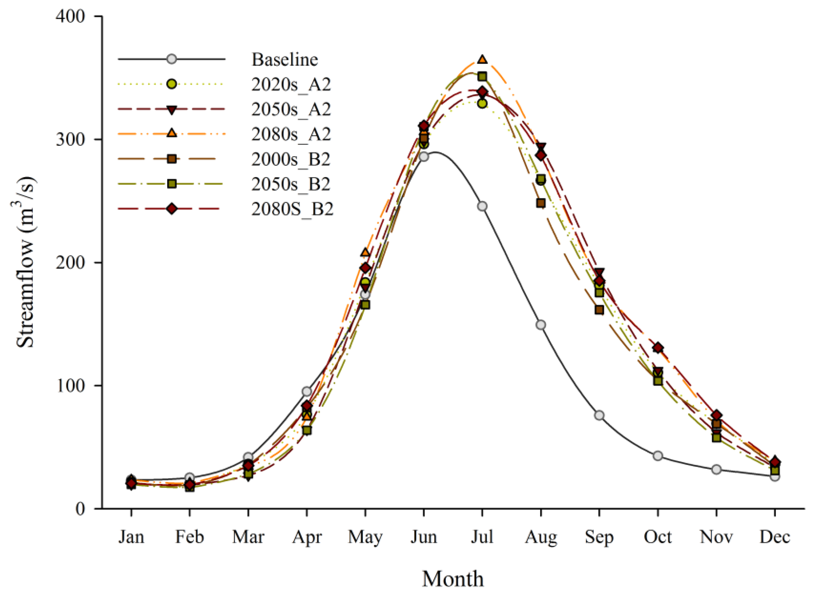
• Mean annual flow was projected to increase in the basin under both A2 and B2 scenarios. Noticeable increase in streamflow was predicted for summer and autumn. However, spring and winter showed decrease in flow.
• High and median flows were predicted to increase but low flows were projected to decrease in the future under both scenarios. Flow duration curves showed that the probability of occurrence of flow will be more in the future, relative to the baseline.
• Peaks were predicted to shift from June to July in the future. Similarly, center-of-volume date, a date at which half of the annual water passes, might get delayed by about 9–17 days in the basin under both A2 and B2.

The overall conclusion of the study is that the Kunhar basin is likely to face more floods and droughts in the future due to the projected increase in high flows and decrease in low flows. Many temporal and magnitudinal variations in peak flows would be faced in the basin. This can create many problems for the policy makers and managers of water resources if they do not consider the impacts of changing climate in the basin. For further studies of the basin, we recommend the use of different GCMs so as to cover the range of uncertainties related to GCMs and to explore a wider range of possible impacts of climate change on water resources in the basin.

Limitations of the Study

In the present study, the impact of climate change on the water resources of the Kunhar River basin were assessed by using only single GCM (HadCM3), although it is suggested that more than one GCM should be used to cover the uncertainties related to GCM outputs. Only two meteorological stations are available in the basin, an indication of the data scarcity of the basin. The scarcity of data can cause a lower level of performance by a hydrological model during the calibration and validation processes. Land cover and soil properties were considered constant throughout the simulation period; such an assumption can affect the projections of streamflow in the basin.

References

1. Mahmood, R.; Babel, M.S. Evaluation of sdsm developed by annual and monthly sub-models for downscaling temperature and precipitation in the jhelum basin, pakistan and india. Theor. Appl. Climatol. 2013, 113, 27–44. [Google Scholar] [CrossRef]
2. Chu, J.; Xia, J.; Xu, C.Y.; Singh, V. Statistical downscaling of daily mean temperature, pan evaporation and precipitation for climate change scenarios in haihe river, China. Theor. Appl. Climatol. 2010, 99, 149–161. [Google Scholar] [CrossRef]
3. Intergovernmental Panel on Climate Change (IPCC). Climate Change 2013: The Physical Science Basis; Contribution of Working Group I to the Fifth Assessment Report of the Intergovernmental Panel on Climate Change; Cambridge University Press: Cambridge, UK; New York, NY, USA, 2013; p. 1535. [Google Scholar]
4. Solomon, S.; Qin, D.; Manning, M.; Chen, Z.; Marquis, M.; Averyt, K.B.; Tignor, M.; Miller, H.L. (Eds.) Climate Change 2007: The Physical Science Basis; Contribution Of Working Group I to the Fourth Assessment Report of the Intergovernmental Panel on Climate Change; Cambridge University Press: Cambridge, UK, 2007.
5. Khattak, M.S.; Babel, M.S.; Sharif, M. Hydro-meteorological trends in the upper indus river basin in Pakistan. Clim. Res. 2011, 46, 103–119. [Google Scholar] [CrossRef]
6. Ma, Z.Z.; Wang, Z.J.; Xia, T.; Gippel, C.J.; Speed, R. Hydrograph-based hydrologic alteration assessment and its application to the Yellow River. J. Environ. Inform. 2014, 23, 1–13. [Google Scholar] [CrossRef]
7. Yang, W.; Yang, Z.F. Evaluation of sustainable environmental flows based on the valuation of ecosystem services: A case study for the Baiyangdian Wetland, China. J. Environ. Inform. 2014, 24, 90–100. [Google Scholar] [CrossRef]
8. Zhang, X.C.; Liu, W.Z.; Li, Z.; Chen, J. Trend and uncertainty analysis of simulated climate change impacts with multiple GCMs and emission scenarios. Agric. Forest Meteor. 2011, 151, 1297–1304. [Google Scholar] [CrossRef]
9. Wang, H.; Zhang, M.; Zhu, H.; Dang, X.; Yang, Z.; Yin, L. Hydro-climatic trends in the last 50 years in the lower reach of the Shiyang River Basin, NW China. Catena 2012, 95, 33–41. [Google Scholar] [CrossRef]
10. Dhital, Y.; Tang, Q.; Shi, J. Hydroclimatological changes in the Bagmati River Basin, Nepal. J. Geogr. Sci. 2013, 23, 612–626. [Google Scholar] [CrossRef]
11. Gleick, P. Regional hydrologic consequences of increases in atmospheric CO2 and other trace gases. Climatic Change 1987, 10, 137–160. [Google Scholar] [CrossRef]
12. Jordan, Y.C.; Ghulam, A.; Chu, M.L. Assessing the impacts of future urban development patterns and climate changes on total suspended sediment loading in surface waters using geoinformatics. J. Environ. Inform. 2014, 24, 65–79. [Google Scholar] [CrossRef]
13. Akhtar, M.; Ahmad, N.; Booij, M.J. The impact of climate change on the water resources of Hindukush–Karakorum–Himalaya region under different glacier coverage scenarios. J. Hydrol. 2008, 355, 148–163. [Google Scholar] [CrossRef]
14. Jetly, R. Pakistan in Regional and Global Politics; Taylor & Francis: New Dehli, India, 2012. [Google Scholar]
15. Connor, R. The United Nations World Water Development Report 2015: Water for a Sustainable World; UNESCO Publishing: Paris, France, 2015. [Google Scholar]
16. Gebremeskel, S.; Liu, Y.B.; de Smedt, F.; Hoffmann, L.; Pfister, L. Analysing the effect of climate changes on streamflow using statistically downscaled gcm scenarios. Int. J. River Basin Manag. 2005, 2, 271–280. [Google Scholar] [CrossRef]
17. Wilby, R.L.; Hay, L.E.; Gutowski, W.J.; Arritt, R.W.; Takle, E.S.; Pan, Z.; Leavesley, G.H.; Martyn, P.C. Hydrological responses to dynamically and statistically downscaled climate model output. Geophys. Res. Lett. 2000, 27, 1199–1202. [Google Scholar] [CrossRef]
18. Hay, L.E.; Wilby, R.L.; Leavesley, G.H. A comparison of delta change and downscaled GCM scenarios for three mountainous basins in The United States. J. Am. Water Resour. Assoc. 2000, 36, 387–397. [Google Scholar] [CrossRef]
19. Ahmad, Z.; Hafeez, M.; Ahmad, I. Hydrology of mountainous areas in the upper Indus Basin, Northern Pakistan with the perspective of climate change. Environ. Monit. Assess. 2012, 184, 5255–5274. [Google Scholar] [CrossRef] [PubMed]
20. Shrestha, M.; Koike, T.; Hirabayashi, Y.; Xue, Y.; Wang, L.; Rasul, G.; Ahmad, B. Integrated simulation of snow and glacier melt in water and energy balance-based, distributed hydrological modeling framework at Hunza River Basin of Pakistan Karakoram region. J. Geophys. Res. Atmos. 2015. [Google Scholar] [CrossRef]
21. Bocchiola, D.; Diolaiuti, G.; Soncini, A.; Mihalcea, C.; D’Agata, C.; Mayer, C.; Lambrecht, A.; Rosso, R.; Smiraglia, C. Prediction of future hydrological regimes in poorly gauged high altitude basins: The case study of the upper Indus, Pakistan. Hydrol. Earth Syst. Sci. 2011, 15, 2059–2075. [Google Scholar] [CrossRef]
22. Meenu, R.; Rehana, S.; Mujumdar, P.P. Assessment of hydrologic impacts of climate change in Tunga-Bhadra river basin, India with HEC-HMS and SDSM. Hydrol. Process. 2012, 27, 1572–1589. [Google Scholar] [CrossRef]
23. Verma, A.; Jha, M.; Mahana, R. Evaluation of HEC-HMS and WEPP for simulating watershed runoff using remote sensing and geographical information system. Paddy Water Environ. 2010, 8, 131–144. [Google Scholar] [CrossRef]
24. Yimer, G.; Jonoski, A.; Griensven, A.V. Hydrological response of a catchment to climate change in the Upper Beles River Basin, Upper Blue Nile, Ethiopia. Nile Basin Water Eng. Sci. Mag. 2009, 2, 49–59. [Google Scholar]
25. García, A.; Sainz, A.; Revilla, J.A.; Álvarez, C.; Juanes, J.A.; Puente, A. Surface water resources assessment in scarcely gauged basins in the north of Spain. J. Hydrol. 2008, 356, 312–326. [Google Scholar] [CrossRef]
26. Munyaneza, O.; Mukubwa, A.; Maskey, S.; Uhlenbrook, S.; Wenninger, J. Assessment of surface water resources availability using catchment modelling and the results of tracer studies in the mesoscale Migina Catchment, Rwanda. Hydrol. Earth Syst. Sci. 2014, 18, 5289–5301. [Google Scholar] [CrossRef]
27. Babel, M.; Bhusal, S.; Wahid, S.; Agarwal, A. Climate change and water resources in the Bagmati River Basin, Nepal. Theor. Appl. Climatol. 2014, 115, 639–654. [Google Scholar] [CrossRef]
28. Wilby, R.L.; Dawson, C.W.; Barrow, E.M. SDSM—A decision support tool for the assessment of regional climate change impacts. Environ. Model. Softw. 2002, 17, 145–157. [Google Scholar] [CrossRef]
29. Gordon, C.; Cooper, C.; Senior, C.A.; Banks, H.; Gregory, J.M.; Johns, T.C.; Mitchell, J.F.B.; Wood, R.A. The simulation of sst, sea ice extents and ocean heat transports in a version of the hadley centre coupled model without flux adjustments. Clim. Dyn. 2000, 16, 147–168. [Google Scholar] [CrossRef]
30. IPCC. Emissions Scenarios: A Special Report of Working Group III; Cambridge University Press: Cambridge, UK, 2000; p. 570. [Google Scholar]
31. Agarwal, C.S.; Garg, P.K. Textbook on Remote Sensing: In Natural Resources Monitoring and Management; A H Wheeler Publishing Co Ltd: New Delhi, India, 2002. [Google Scholar]
32. Singh, D.; Gupta, R.D.; Jain, S. Assessment of impact of climate change on water resources in a hilly river basin. Arab. J. Geosci. 2015, 8, 10625–10646. [Google Scholar] [CrossRef]
33. Ghoraba, S.M. Hydrological modeling of the simly dam watershed (Pakistan) using GIS and SWAT model. Alex. Eng. J. 2015, 54, 583–594. [Google Scholar] [CrossRef]
34. Leghari, M.K.; Waheed, S.B.; Leghari, M.Y. Ecological study of algal flora of Kunhar River, Pakistan. Pak. J. Bot. 2001, 33, 629–636. [Google Scholar]
35. De Scally, F.A. Relative importance of snow accumulation and monsoon rainfall data for estimating annual runoff, Jhelum Basin, Pakistan. Hydrol. Sci. J. 1994, 39, 199–216. [Google Scholar] [CrossRef]
36. Hussain, M.; Shah, G.M.; Khan, M.A. Traditional medicinal and economic uses of Gymnosperms of Kaghan valley, Pakistan. Ethnobot. Leafl. 2006, 10, 72–81. [Google Scholar]
37. Pakistan Ministry of Water and Power (PMWP). Executive Summary, Pakistan Water Sector Strategy; PMWP: Islamabad, Pakistan, 2002; p. 24.
38. Ahmad, I.; Ambreen, R.; Sun, Z.; Deng, W. Winter-spring precipitation variability in Pakistan. Am. J. Clim. Chang. 2015, 4, 115–139. [Google Scholar] [CrossRef]
39. Mahmood, R.; Babel, M.S.; Jia, S. Assessment of temporal and spatial changes of future climate in the Jhelum river basin, Pakistan and India. Weather Clim. Extrem. 2015, 10, 40–55. [Google Scholar] [CrossRef]
40. Hydrologic Modeling System HEC-HMS; Institute for Water Resources: Davis, CA, USA, 2010.
41. Van Liew, M.W.; Garbrecht, J. Hydrologic simulation of the Little Washita river experimental watershed using SWAT1. J. Am. Water Resour. Assoc. 2003, 39, 413–426. [Google Scholar] [CrossRef]
42. HEC-ResSim Reservoir System Simulation User’s Manual; Hydrologic Engineering Center: Davis, CA, USA, 2007; p. 512.
43. Mahmood, R.; Babel, M.S. Future changes in extreme temperature events using the statistical downscaling model (SDSM) in the trans-boundary region of the Jhelum river basin. Weather Clim. Extrem. 2014, 5–6, 56–66. [Google Scholar] [CrossRef]
44. Stewart, I.T.; Cayan, D.R.; Dettinger, M.D. Changes toward earlier streamflow timing across western North America. J. Clim. 2005, 18, 1136–1155. [Google Scholar] [CrossRef]