Land Use/Cover Change Impacts on Water Table Change over 25 Years in a Desert-Oasis Transition Zone of the Heihe River Basin, China

Abstract

Groundwater resources are becoming the primary factor for maintaining life in arid areas. Understanding land use/cover change and its effect on groundwater depth would enhance land use and groundwater management for typical desert-oasis transition zones. Reduction of groundwater recharge and increase of groundwater exploitation during 1985 and 2010 led to the decrease of groundwater depth in Linze County. The region with groundwater depth less than 5 m decreased by 187 km² from 1985 to 2010 as a result of industrial growth, agricultural and economic development. Land use has undergone significant spatial and temporal changes. Farmland and built up land expanded by 53.02% and 30.91%, respectively. The expansion of farmland reached a peak between 1996 and 2005 with an increasing rate of 25.70%, while areas of grassland, woodland, water body and unused land decreased, and the decreasing rate was 9.38%, 58.35% and 19.81%. From 1985 to 2010, the groundwater depth rose slightly (0–1.2 m) in the edge of desert (24.21 km²), which was caused by the surrounding farmland irrigation recharge. The drawdown range of groundwater depth between 0 and 3 m was distributed in the central oasis, which was caused by the expansion of farmland and degradation of natural vegetation. This study aims to provide a basis for the reasonable utilization of water resources, the formation of management strategies, as well as to provide ecosystem stability and sustainable development of oases in the study area.

1. Introduction

In arid and semi-arid areas, groundwater resource is a sensitive factor of ecological environment [1,2,3,4], and helps to maintain vegetation in naturally occurring desert oases, as well as the social stability and economy in this desert environment [1,5]. Therefore, an accurate understanding of the spatiotemporal variability of groundwater is very important for making reasonable plans of oasis development and ensuring ecosystem sustainability [6].

The environmental effect of land use/cover change has been a popular research topic [7] in recent studies. The International Geosphere-Biosphere Program (IGBP) and the International Human Dimension Program (IHDP) have taken the relationship between Biosphere Aspects of the Hydrological Cycle (BAHC) and the land use and land cover changes as the core plans. Moreover, in the LUCC research plans established by IGBP and IHDP, one core problem is to understand the impact of the regional land use and land cover changes on hydrological process and water resources. LUCC is a driving factor for changes of regional climate and hydrology [8,9,10]. It can significantly affect hydrological processes (the rain interception of vegetation, the infiltration capacities of soil and the evaporation rate at the surface) and runoff mechanisms, and thus influence groundwater recharge and discharge [11,12,13]. A better understanding of the impact of LUCC on underground hydrological processes will provide a scientific basis for planning and managing water resources [9,14,15]. As an important part of the regional hydrologic cycle, groundwater is closely connected with land use and has strong response to LUCC in the basin [6,16,17,18,19].

Geostatistics is useful for capturing the spatial heterogeneity and spatial pattern of environmental variables. It has been well applied in soil science, ecology, and other fields; geostatistics has also been applied in groundwater modeling and spatial variation recently gradually. Geostatistical methods are good tools for deriving the long term trends of the groundwater [20]. Theodossiou and Latinopoulos analyzed the groundwater level of the Upper Anthemountas basin in northern Greecein by using kriging interpolation, and estimated the interpolation precision by using cross validation method [21]. Seyed and Abbas analyzed the groundwater level drop and groundwater level fluctuations for the Darab plain which was located in south-east of Fars province, south of Iran, by using ordinary and universal kriging methods with cross-validation; then they evaluated kriging and cokriging methods for mapping the groundwater depth across the plain in different climatic conditions, their results showed that co-kriging approach was more accurate than kriging in mapping the groundwater depth [22,23]. Deepesh Machiwal et al. modeled the spatial and temporal variations of groundwater levels based on monthly groundwater-level data of 50 sites for the 36-month period (May 2006–June 2009) obtained from a semi-arid hard-rock groundwater basin of Western India by using geostatistics and GIS techniques [24]. Ma et al. simulated the groundwater depth of the heartland in southern Kansas City by using ordinary kriging methods to estimate the initial conditions of the groundwater level and the terrain, and using co-kriging to estimate the initial conditions of the fresh-saline groundwater interface [25]. Previous studies as mentioned above just analyzed the temporal and spatial variability of groundwater. The studies in regarding the impact of land cover change on groundwater depth are lacking.

Coupled with the reduction of surface water diversion under the implementation of the Ecological Water Transfer Project and land use change, groundwater exploitation increased from 1.16 × 10⁸ m³ in 1990 to 3.68 × 10⁸ m³ in 2009, exceeding the annual limit value 3.6 × 10⁸ m³, which showed that groundwater was in a negative balance state. Accordingly, the groundwater depth in the middle reaches of Heihe River basin generally decreased, and the reserves decreased by nearly 1.86 × 10¹⁰ m³ mainly due to land use change. For these reasons, groundwater and LUCC in the middle reaches of Heihe River basin should be widely studied. Our study aims to explore the response of groundwater depth change to land cover change in the middle reaches of Heihe River basin.

The major objectives are (1) to analyze the spatial pattern and map groundwater level differences for the observation period; (2) to evaluate changes in the persistence of groundwater level differences with geostatistical methods; (3) to examine the temporal and spatial distribution trend in land cover by using historical remote sensing data; and (4) to explore the effect of land use change on groundwater depth.

2. Materials and Methods

2.1. Study Area

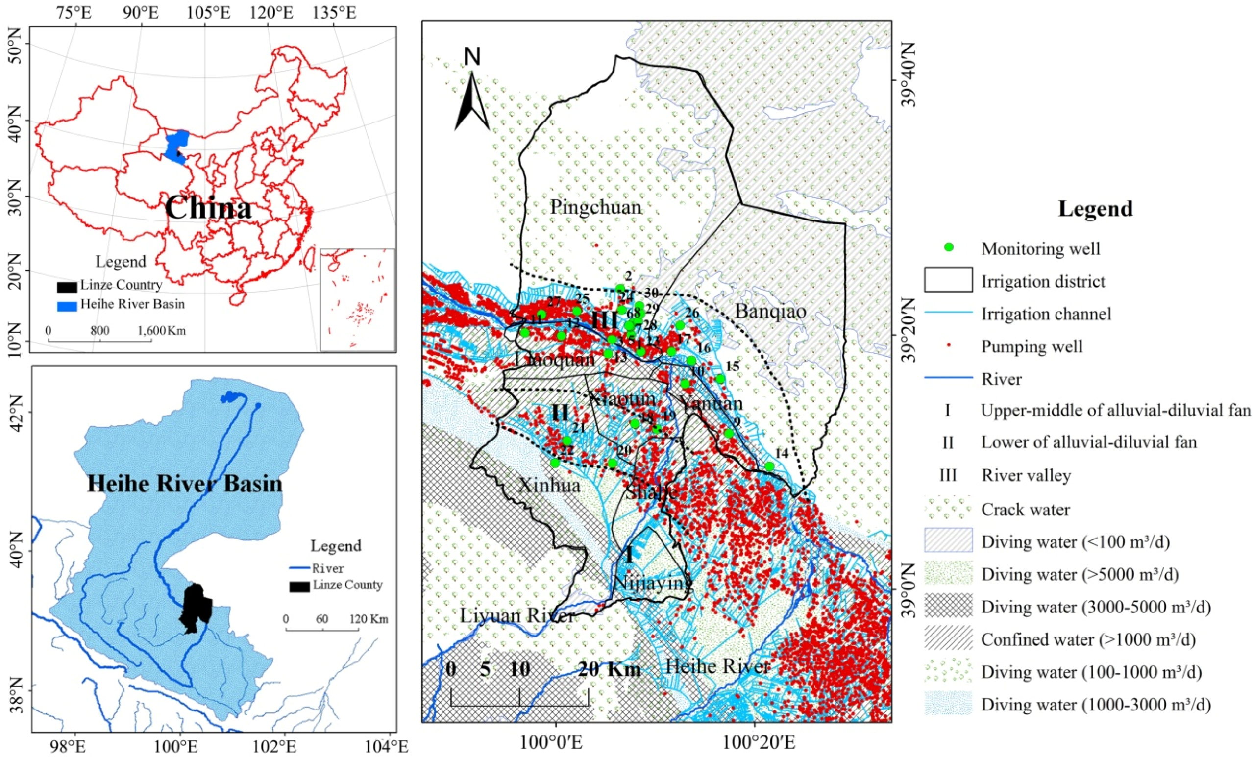
Linze County (38°57′–39°42′ N, 99°51′–100°30′ E), which geographically belongs to the middle reaches of the Heihe River basin, is located in the central part of Hexi Corridor (Figure 1). The county covers an area of 2680 km². The altitude is between 1350 m and 2084 m above sea-level. The landscape is comprised of piedmont alluvial and diluvial gravel plain in the south and fine-grained soil plain in the central part. With the implementation of the Ecological Water Transfer Project (EWTP) of the Heihe River Basin from 2001, unified allocation of water resources is processed through the entire basin. The river water usage in the middle reaches has been considerably limited; as a result, the land use undergoes a noticeable change. With the expansion of the oasis agriculture in the middle reaches of Heihe River Basin, the irrigation area increased from 17.45 × 10⁴ hm² in 1990 to 24.04 × 10⁴ hm² in 2009. Based on the topographic units, the study area is divided into three hydro-geological units from south to north: the upper-middle part of the alluvial-diluvial fan in the south, the lower part of the alluvial-diluvial fan between the southern part and the central part, and the river valley plain in the middle. The aquifer is composed of single aquifer, multi-layer and confined aquifer [26]. Groundwater mainly received the vertical infiltration recharge of river (flood, 0.6 × 10⁸ m³/a) and irrigation water (drainage system and cultivated land, 0.8 × 10⁸ m³/a), which accounted for approximately 80% of the total recharge (1.75 × 10⁸ m³/a); the infiltration recharge of lateral flow (0.3 × 10⁸ m³/a), precipitation and condensation water (0.05 × 10⁸ m³/a) accounted for approximately 20% [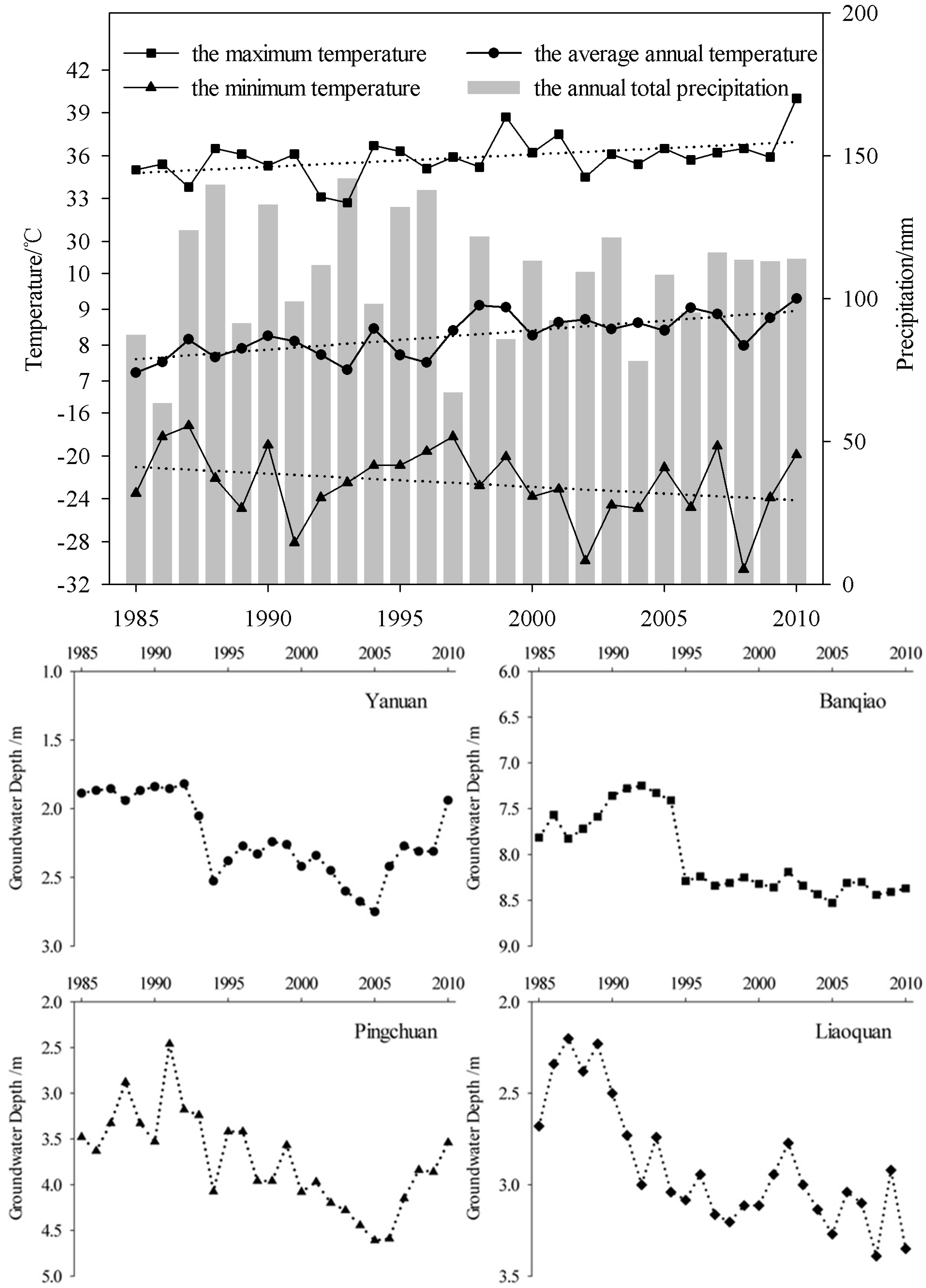27]. The water overflow of springs distributed in the Xiaotun irrigation district and the Pingchuan irrigation district, evaporation and artificial exploitation are the main drainage mechanisms of groundwater. The annual change of groundwater depth for four representative monitoring wells was showed in Figure 2. The results presented that the groundwater depth in the study area decreased gradually.

Figure 1. The study area and the distribution of observation wells in Linze County in the Heihe River basin, China.

Figure 1. The study area and the distribution of observation wells in Linze County in the Heihe River basin, China.

Based on the data from the meteorological observation field in the Linze Inland River Basin Research Station, Chinese Academy of Sciences (CAS), the average annual temperature of the study area is 8.27 °C, and the maximum and minimum temperatures are 35.9 °C and −22.6 °C, respectively (Figure 2). The annual total precipitation is 109 mm (Figure 2) and is concentrated between July and September, which accounts for 65% of the annual total precipitation. The average annual potential evaporation is up to 2390 mm. The county is divided into eight irrigation districts, which are Pingchuan, Banqiao, Yanuan, Liaoquan, Xiaotun, Xinhua, Shahe and Nijiaying, respectively. The irrigation districts are mainly irrigated by the mainstream of Heihe River and its tributary, Liyuan River. The irrigation agriculture in the study area was highly developed. Crops planted here include wheat, seed maize, tomato, cotton, and greenhouse vegetables. There is a complete irrigation system with more than 300 main canals and branch canals. The number of pumping wells demonstrates a rapid increasing trend in the 1990s and 2000s (Table 1).

Figure 2. Change of annual total precipitation, annual temperature and annual groundwater depth between 1985 and 2010.

Figure 2. Change of annual total precipitation, annual temperature and annual groundwater depth between 1985 and 2010.

Table 1. The temporal series proportions of water resources between surface water irrigation and groundwater exploitation for each irrigation districts in three periods.

Irrigation District	Canal Irrigation (108 m3)			Groundwater (108 m3)			Well Number
	1985–1989	1990–1999	2000–2010	1985–1989	1990–1999	2000–2010	1985–1989	1990–1999	2000–2010
Shahe	0.20	0.44	0.27	0.03	0.10	0.23	12	53	129
Yanuan	0.30	0.63	0.44	0.006	0.018	0.088	8	16	79
Liaoquan	0.40	0.96	0.58	0.004	0.022	0.067	17	55	191
Banqiao	0.40	1.05	1.13	0.002	0.002	0.025	13	15	84
Pingchuan	0.60	1.05	0.72	0.018	0.075	0.177	50	144	337

Table 1. The temporal series proportions of water resources between surface water irrigation and groundwater exploitation for each irrigation districts in three periods.

Irrigation District	Canal Irrigation (108 m3)			Groundwater (108 m3)			Well Number
	1985–1989	1990–1999	2000–2010	1985–1989	1990–1999	2000–2010	1985–1989	1990–1999	2000–2010
Shahe	0.20	0.44	0.27	0.03	0.10	0.23	12	53	129
Yanuan	0.30	0.63	0.44	0.006	0.018	0.088	8	16	79
Liaoquan	0.40	0.96	0.58	0.004	0.022	0.067	17	55	191
Banqiao	0.40	1.05	1.13	0.002	0.002	0.025	13	15	84
Pingchuan	0.60	1.05	0.72	0.018	0.075	0.177	50	144	337

2.2. Data

Groundwater data from 30 monitoring wells during 1985 and 2010 maintained by the Gansu Provincial Bureau of Hydrology and the Linze Inland River Basin Research Station, Chinese Academy of Sciences (CAS) were collected. The monitoring well distribution is shown in Figure 1 and Table 2. The depth of the groundwater table in January is determined on behalf of the annual groundwater depth because January is the month in which the groundwater table is relative the least impacted by irrigation. January measurements are the average of three time measurements, and the measurements are manually taken at 1, 11 and 21 per month by using tape. The irrigation data were collected from annual water resource management reports (1985–2010) published by the Zhangye Municipal Bureau of Water Conservancy. The meteorological data were obtained from the meteorological observation field in the Linze Inland River Basin Research Station, CAS.

Table 2. The physical and hydro-geological conditions of the study area, together with the monitoring wells in different sub-areas [28].

Area Code	Subarea	Distribution and Natural Conditions	Hydro-Geological and Irrigation Conditions	Monitoring Well Code
I	Upper-middle of alluvial-diluvial fan	The River Valley alluvial plain, annual precipitation is 120–300 mm	Single unconfined aquifer, The groundwater depth is >30 m, river irrigation	19–21
II	Lower of alluvial-diluvial fan	The intersection zone of River Valley alluvial plain and fine-grained soil plain, annual precipitation is 0–255 mm	Transition from single aquifer to multi-layer and confined aquifer, The groundwater depth is during 5–30 m, mixed irrigation	17, 18
III	River valley	River Valley alluvial plain, annual precipitation is 60–130 mm	Multi-layer and confined aquifer, the groundwater depth is <10 m, mixed irrigation	1–16, 22–30

Table 2. The physical and hydro-geological conditions of the study area, together with the monitoring wells in different sub-areas [28].

Area Code	Subarea	Distribution and Natural Conditions	Hydro-Geological and Irrigation Conditions	Monitoring Well Code
I	Upper-middle of alluvial-diluvial fan	The River Valley alluvial plain, annual precipitation is 120–300 mm	Single unconfined aquifer, The groundwater depth is >30 m, river irrigation	19–21
II	Lower of alluvial-diluvial fan	The intersection zone of River Valley alluvial plain and fine-grained soil plain, annual precipitation is 0–255 mm	Transition from single aquifer to multi-layer and confined aquifer, The groundwater depth is during 5–30 m, mixed irrigation	17, 18
III	River valley	River Valley alluvial plain, annual precipitation is 60–130 mm	Multi-layer and confined aquifer, the groundwater depth is <10 m, mixed irrigation	1–16, 22–30

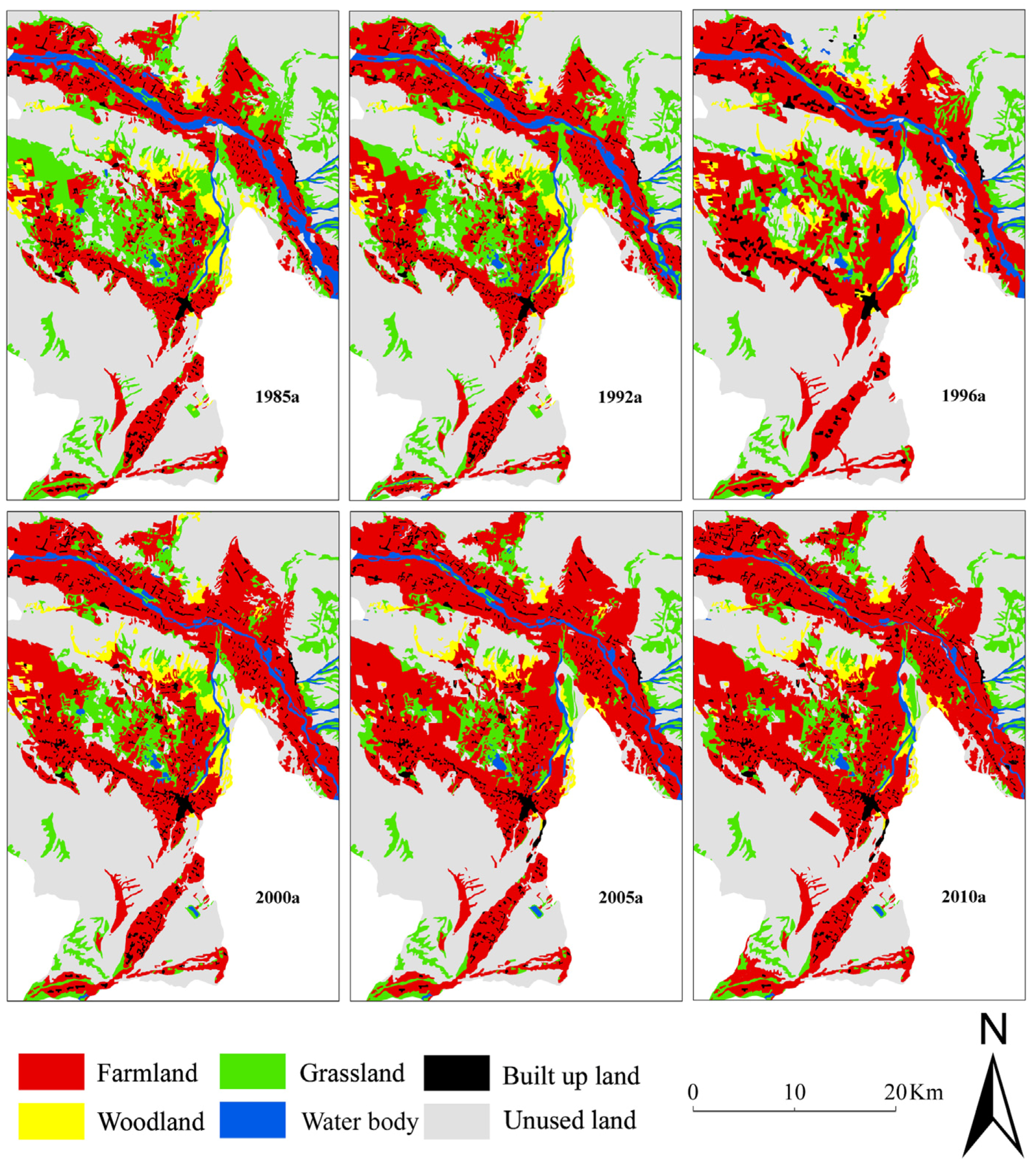
The remote sensing data include five land use/cover classification maps (1985, 1996, 2000, 2005 and 2010) and Landsat_5 Thematic Mapper (TM) satellite image (Path/Row 164 and 38, 28 August 1992) under cloud-free conditions from the United States Geological Survey (USGS). The land use data in 1992 was clipped directly from the 1:100,000 scale land use database developed by the Chinese Academy of Sciences (CAS) [29]. Preprocessing of the satellite image prior to image classification and change detection is essential and commonly comprises a series of sequential operations, including atmospheric correction or normalization, geometric correction, and image enhancement [30]. The land use classification was conducted through visual interpretation to guarantee consistency and accuracy in the data processing. By field surveys and random sample checks, we confirmed that the overall interpretation accuracy of the land use classification was reliable. All maps and images were presented in the Universal Transverse Mercator (UTM) coordinate system referenced to the 1984 World Geodetic System (WGS84). According to the classification system of national land-use status [31] and land-use characteristics in Linze County, landuse patterns in the study area have been divided into 6 types: farmland, woodland, grassland, water body, built up land and unused land.

2.3. Geostatistics

We analyzed the spatial distribution of the groundwater depth and the variability of the groundwater during the period between 1985 and 2010 in the study area using the geostatistics method based on the groundwater depths. Geostatistics is useful for capturing the spatial heterogeneity and spatial pattern of environmental variables.

Geostatistical theory is based on a stochastic model which allows the derivation of optimal predictions at random points in the considered region. It allows us to take into account spatial correlation between neighboring observations and includes different approaches spanning from conditional estimator to simulation, either parametric or indicator approach [32]. It aims at providing quantitative descriptions of natural variables distributed in space and time [33,34]. Geostatistics can be used for the better management and conservation of water resources and sustainable development of any area [20,35], and geostatistical methods are good tools for water resources management and can effectively be used to derive the long term trends of the groundwater [20]. Several studies used geostatistics for optimizing a groundwater monitoring network [21,36,37,38,39]. Christakos performed the geostatistical analysis on water table elevation of about 70 wells in Kansas [40]. Ahmadi and Sedghamiz applied geostatistics for spatial and temporal analyses of the groundwater levels in Darab plain of Iran [22,23]. Based on the above studies, geostatistical methods has been proved as an applicable and reliable tool to reveal stochastic structure of groundwater level variations in space and time, and for better management and conservation of water resources.

The semi-variance method and Kriging interpolation are basic methods of geostatistics [34,41]. Semi-variance is an autocorrelation statistic defined as:

$$r(h)=\frac{1}{2N(h)}{\displaystyle \sum _{i=1}^{N(h)}{\left[z(x_i)-z(x_i+h)\right]}^2}$$

(1)

where r(h) is the semivariance for interval distance class h; Z(x_i) is the measured sample value at point x_i; Z(x_i + h) is the measured sample value at point x_i + h; and N(h) is the total number of sample couples for the lag interval h.

Prior to the geostatistical estimation, we require a model that enables us to compute a variogram value for any possible sampling interval. The most commonly used models are spherical, exponential, Gaussian, and pure nugget effect [34]. Assuming a normal distribution for the groundwater depth, a spatial interpolation model was created based on the regionalized variables z(x_i) and z(x_i + h). The experimental variogram was fitted by an exponential model, that is:

$$r(h)=\{\begin{array}{l}0h=0\\ c_0+c(1-e^{-\frac{h}{a}})h>0\end{array}$$

(2)

where r(h) is the semi-variance for interval distance class h, and h is the lag interval; C₀ is the nugget variance (C₀ ≥ 0); C is the structural variance(C ≥ C₀); and a is the range parameter. In the case of the exponential model, the effective range A = 3a, which is the distance at which the sill (C + C₀) is within 5% of the asymptote (the sill never meets the asymptote in the exponential model).

The adequacy and validity of the developed variogram model was tested satisfactorily by a technique called cross-validation. This test allows us to assess the goodness of fitting (avoid sufficiency) of the variogram model (type, parameter estimates), the appropriateness of neighborhood and type of kriging used. Interpolated and observed values are compared, and the model that yields the most accurate predictions is retained [34,42]. The fitness of the semi-variogram model is evaluated using two parameters: the Residual Sum of Squares (RSS) and coefficient of determination (R²). RSS (RSS > 0) provides an exact measure of how well the model fits the variogram data. The closer the value approaches 0, the better the model fits. The formula of RSS is:

$$RSS={\displaystyle \sum _{i=1}^n{\left[r(h_i)-\widehat{r}(h_i)\right]}^2}$$

(3)

where $\widehat{r}\left(h_i\right)$ is the semi-variance calculated by the theoretical model.

R² is the ratio between the regression sum of squares and the total sum of squares. The closer that the value approaches 1, the better the model fits. The formula of R² is:

$$R^2=\frac{{\displaystyle \sum _{i=1}^n{\left[\widehat{r}(h_i)-\overline{r}(h)\right]}^2}}{{\displaystyle \sum _{i=1}^n{\left[r(h_i)-\overline{r}(h)\right]}^2}}$$

(4)

where $\overline{r}\left(h\right)$ is the average value of the semi-variance.

The GS+ software is then employed to measure geostatistical parameters. Spatial auto-correlation length (range), nugget variance and sill variance are derived from the fitted semi-variogram. The nugget variance (C₀) represents variance caused by random factors in small scale, the sill variance (C₀ + C₁) reflects the variation caused by structural factors in large scale, the ratio of them (GD) can reflect the spatial correlation of groundwater depth. The ratio (GD) can be used to classify the spatial dependence as strong if GD is ≤25%, moderate if it is 25% ≤ GD ≤ 75%, and weak if it is ≥75%. This proportion of spatial structure determines the ratio in which random factors induce spatial variability [43]. The degree of spatial dependence (GD) was calculated as:

$$GD=\frac{C_0}{C_0+C_1}\times 100\%$$

(5)

Kriging is one of the best local estimation methods. It can comprehensively consider the randomness and structure of variables, and estimate the spatial variation of the study object according to the distribution of sampling points and variogram models [40]. Among the different kriging methods, we used ordinary for spatial and temporal analysis. The ordinary kriging method is mainly applied for datasets without and with a trend. Detailed discussions of kriging methods and their descriptions can be found in Goovaerts [42]. The general equation for linear kriging estimation is:

$$Z*({\mathsf{\chi }}_P)={\displaystyle \sum _{i=1}^n{\mathsf{\lambda }}_{i}Z({\mathsf{\chi }}_i)}$$

(6)

To achieve unbiased estimations using ordinary kriging interpolation, the following set of equations should be solved simultaneously.

$${\displaystyle \sum _{i=1}^n{\mathsf{\lambda }}_i\mathsf{\gamma }({\mathsf{\chi }}_i,{\mathsf{\chi }}_j)-\mathsf{\mu }=\mathsf{\gamma }({\mathsf{\chi }}_i,\mathsf{\chi })}$$

(7)

$${\displaystyle \sum _{i=1}^n{\mathsf{\lambda }}_i=1}$$

(8)

where Z*(χ_p) is the kriged value at location χ_p, Z(χ_i) is the known value at location χ_i, λ_i is the weight associated with the data, μ is the Lagrange multiplier, and γ(χ_i,χ_j) is the value of variogram corresponding to a vector with origin in χ_i and extremity in χ_j.

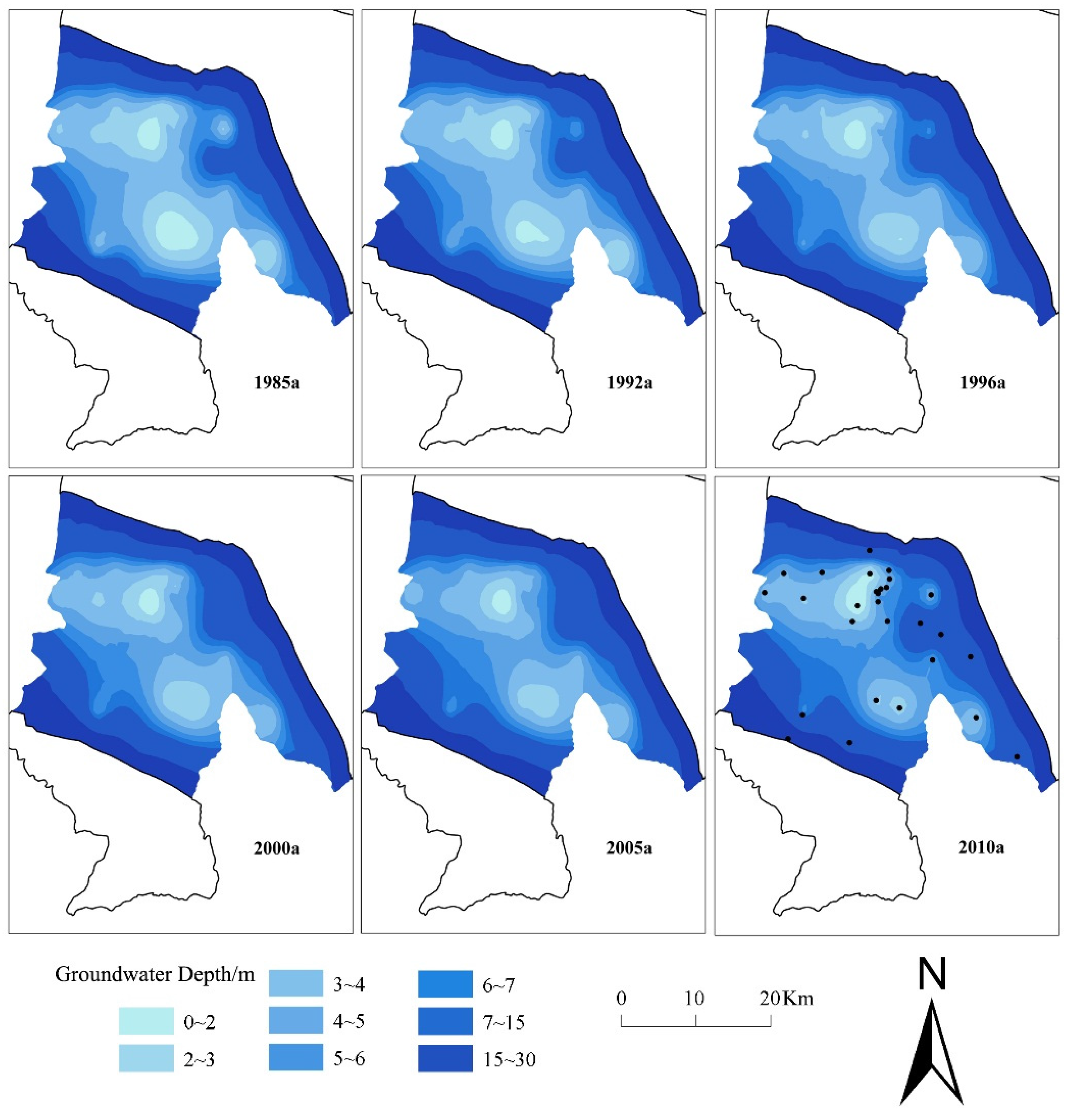
In this paper, the groundwater depth data in six different periods (1985, 1992, 1996, 2000, 2005 and 2010) were transformed into logarithms using the geostatistical analysis module of ArcGIS. Then the logarithms were interpolated using the fitted exponential model and ordinary kriging interpolation to obtain the spatio-temporal variability of groundwater depth in Linze County.

2.4. Remote Sensing and GIS Analysis

Based on the Landsat TM image and five land cover classification maps, the land use/cover types in Linze County were classified into farmland, woodland, grassland, water body, built up land and unused land. Through ArcGIS software, the area of different land use types in 1985, 1992, 1996, 2000, 2005 and 2010 were calculated, and the transition matrix of land use types was generated. The six land use/cover maps and the spatial distribution maps of groundwater depth in the same periods were overlain to compare and analyze the impact of land use/cover change on groundwater depth.

3. Results

3.1. Analysis on the Spatial and Temporal Variations of Groundwater Depth

3.1.1. Development, Prediction and Validation of the Semi-Variogram Model

In this study, the spatial variability of groundwater depth is predicted and simulated by using module of geostatistical analysis and the semivariogram model under ArcGIS. The semivariograms are regressed with exponential functions. The nugget increased significantly during 1985 and 2010, and the sill variance was not obvious. The phenomenon showed that groundwater produced large changes in the small scale caused by random factors (human activities) and little changes at the structural scale. GD values were 5.5%, 12.5%, 12.6%, 14.7%, 12.8%, 15.9%, respectively, which were less than 25% (Table 3). The ratio showed a growing trend, indicating that the effects of human activities were more obvious. The range in 1985 and 2005 was 14910 m and 20580 m, respectively, the maximum correlation distance increased. The ranges of groundwater depth in different years were all small, which showed that the autocorrelation range is small, and the change of groundwater depth had no significant regional differentiation.

Table 3. Parameters of the exponential model for groundwater depth.

Year	Model	Nugget	Sill	GD	Range Parameter/m	R2	RSS
1985	Exponential	0.033	0.598	0.055	14910	0.804	0.050
1992	Exponential	0.076	0.609	0.125	23250	0.747	0.062
1996	Exponential	0.065	0.517	0.126	18240	0.653	0.072
2000	Exponential	0.085	0.577	0.147	28350	0.668	0.072
2005	Exponential	0.063	0.492	0.128	20580	0.627	0.073
2010	Exponential	0.069	0.435	0.159	26690	0.653	0.071

Table 3. Parameters of the exponential model for groundwater depth.

Year	Model	Nugget	Sill	GD	Range Parameter/m	R2	RSS
1985	Exponential	0.033	0.598	0.055	14910	0.804	0.050
1992	Exponential	0.076	0.609	0.125	23250	0.747	0.062
1996	Exponential	0.065	0.517	0.126	18240	0.653	0.072
2000	Exponential	0.085	0.577	0.147	28350	0.668	0.072
2005	Exponential	0.063	0.492	0.128	20580	0.627	0.073
2010	Exponential	0.069	0.435	0.159	26690	0.653	0.071

The RSS were 0.050, 0.062, 0.072, 0.072, 0.073 and 0.071, and R² were 0.804, 0.747, 0.653, 0.668, 0.627 and 0.653. These results revealed that the enactment of the model and parameters are rational, and the regressed results are significant. The high R² and small RSS indicated that groundwater depth could be modeled with a high degree of confidence.

3.1.2. Spatial and Temporal Variations of Groundwater Depth

The spatial distribution maps of groundwater depth (Figure 3) were generated by ordinary kriging in ArcGIS based on the parameters of the exponential model. The groundwater is deeper in the south and north than that in the middle area. The groundwater depth is below 7 m in the river valley.

Table 4 and Table 5 show area changes and the transition matrix of the region with different groundwater depths from 1985 to 2010. The area with groundwater depth below 5 m reduced by 195.14 km² during 25 years, and the decreasing rate was 44.58%. Specifically, the area with groundwater depth of 0–2 m decreased by 21.72 km² (mainly in Xiaotun), which accounted for 66.16%, and the depth range of these regions increased to 2–5 m. The area with groundwater depth of 2–3 m, 3–4 m and 4–5 m, reduced by 78.15 km², 82.38 km² and 2.90 km², respectively, and the decreasing reate was 77.36%, 46.27%, and 2.30%, respectively. The groundwater depth range in these regions increased to 3–6 m, 4–7 m and >5 m, respectively.

Figure 3. Isogram maps of groundwater depth in Linze County (black dots strand for the monitoring wells).

Figure 3. Isogram maps of groundwater depth in Linze County (black dots strand for the monitoring wells).

Table 4. The area change of the regions with respect to groundwater depth from 1985 to 2010 (km²).

Year	Groundwater Depth/m
	0–2	2–3	3–4	4–5	5–6	6–7	>7
1985	32.83	101.01	178.04	125.87	81.34	63.67	429.36
1992	17.97	89.52	171.33	117.63	85.56	70.20	480.41
1996	8.83	60.01	160.59	115.59	99.35	74.52	502.86
2000	7.35	50.08	152.41	121.63	99.55	72.95	522.36
2005	6.56	35.71	127.23	138.53	93.90	85.58	535.65
2010	11.10	22.87	95.67	112.97	119.89	102.40	547.20

Table 4. The area change of the regions with respect to groundwater depth from 1985 to 2010 (km²).

Year	Groundwater Depth/m
	0–2	2–3	3–4	4–5	5–6	6–7	>7
1985	32.83	101.01	178.04	125.87	81.34	63.67	429.36
1992	17.97	89.52	171.33	117.63	85.56	70.20	480.41
1996	8.83	60.01	160.59	115.59	99.35	74.52	502.86
2000	7.35	50.08	152.41	121.63	99.55	72.95	522.36
2005	6.56	35.71	127.23	138.53	93.90	85.58	535.65
2010	11.10	22.87	95.67	112.97	119.89	102.40	547.20

Table 5. The area transition matrix with different ranges of groundwater depth (km²).

	2010	0–2	2–3	3–4	4–5	5–6	6–7	7–15	>15	Total
1985
0–2 m		8.60	5.48	15.34	3.40	-	-	-	-	32.82
2–3		2.50	16.48	45.6	26.60	9.73	0.11	-	-	101.02
3–4		-	0.9	33.69	70.52	56.51	14.83	1.6	-	178.05
4–5		-	0.01	1.04	12.00	48.71	49.10	15.01	-	125.87
5–6		-	-	-	0.45	4.79	35.21	40.90	-	81.35
6–7		-	-	-	-	0.16	2.83	60.69	-	63.68
7–15		-	-	-	-	-	0.33	196.18	49.16	245.67
>15		-	-	-	-	-	-	0.17	183.52	183.69
Total		11.10	22.87	95.67	112.97	119.90	102.41	314.55	232.68	1012.15

Table 5. The area transition matrix with different ranges of groundwater depth (km²).

	2010	0–2	2–3	3–4	4–5	5–6	6–7	7–15	>15	Total
1985
0–2 m		8.60	5.48	15.34	3.40	-	-	-	-	32.82
2–3		2.50	16.48	45.6	26.60	9.73	0.11	-	-	101.02
3–4		-	0.9	33.69	70.52	56.51	14.83	1.6	-	178.05
4–5		-	0.01	1.04	12.00	48.71	49.10	15.01	-	125.87
5–6		-	-	-	0.45	4.79	35.21	40.90	-	81.35
6–7		-	-	-	-	0.16	2.83	60.69	-	63.68
7–15		-	-	-	-	-	0.33	196.18	49.16	245.67
>15		-	-	-	-	-	-	0.17	183.52	183.69
Total		11.10	22.87	95.67	112.97	119.90	102.41	314.55	232.68	1012.15

3.2. Land Use/Cover Changes Analysis

The land use/cover maps of Linze County in 1985, 1992, 1996, 2000, 2005 and 2010 were used to obtain area changes of land use types (Figure 4, Table 6 and Table 7) and analyze the mutual transformation (i.e., transition area, intensity, direction and the spatial position of conversion) among the six land use types (Figure 5).

Table 6. Land use/cover change of Linze County.

	Year	Farmland	Woodland	Grassland	Water Body	Built up Land
Area (km2)	1985	316.03	39.49	314.96	51.28	29.60
	1992	348.64	39.22	289.77	43.87	29.79
	1996	374.15	51.31	235.61	43.39	31.84
	2000	425.36	37.27	226.37	33.99	34.07
	2005	476.46	25.72	214.02	34.62	34.36
	2010	483.58	26.06	216.28	29.26	38.75
Area Change (%)	1985–1992	10.32	−0.68	−8.00	−14.45	0.64
	1992–1996	7.32	30.83	−18.69	−1.09	6.88
	1996–2000	13.69	−27.36	−3.92	−21.66	7.00
	2000–2005	12.01	−30.99	−5.46	1.85	0.85
	2005–2010	1.49	1.32	1.06	−15.48	12.78
	1985–2010	53.02	−34.01	−31.33	−42.94	30.91

Table 6. Land use/cover change of Linze County.

	Year	Farmland	Woodland	Grassland	Water Body	Built up Land
Area (km2)	1985	316.03	39.49	314.96	51.28	29.60
	1992	348.64	39.22	289.77	43.87	29.79
	1996	374.15	51.31	235.61	43.39	31.84
	2000	425.36	37.27	226.37	33.99	34.07
	2005	476.46	25.72	214.02	34.62	34.36
	2010	483.58	26.06	216.28	29.26	38.75
Area Change (%)	1985–1992	10.32	−0.68	−8.00	−14.45	0.64
	1992–1996	7.32	30.83	−18.69	−1.09	6.88
	1996–2000	13.69	−27.36	−3.92	−21.66	7.00
	2000–2005	12.01	−30.99	−5.46	1.85	0.85
	2005–2010	1.49	1.32	1.06	−15.48	12.78
	1985–2010	53.02	−34.01	−31.33	−42.94	30.91

Figure 4. Land use/cover change pattern of Linze County from 1985 to 2010.

Figure 4. Land use/cover change pattern of Linze County from 1985 to 2010.

Table 7. Land use/cover of different irrigation districts in 1985 and 2010 (km²).

Year	Irrigation District	Farmland	Woodland	Grassland	Water	Built up Land	Unused Land	Total
1985	Banqiao	46.14	2.52	140.29	20.95	3.40	566.27	779.57
	Nijiaying	25.60	0.06	3.43	0.00	3.32	49.34	81.75
	Liaoquan	34.79	1.84	11.41	9.51	2.89	58.47	118.91
	Pingchuan	51.55	3.70	17.49	6.89	3.86	888.37	971.86
	Xiaotun	29.31	16.25	44.15	3.31	2.84	28.99	124.85
	Xinhua	63.25	7.31	75.48	0.75	5.82	270.87	423.48
	Shahe	35.89	7.10	10.15	2.69	5.17	47.13	108.13
	Yanuan	29.30	1.67	12.32	8.11	2.36	17.34	71.10
	toltal	315.83	40.45	314.72	52.21	29.66	1926.78	2679.65
2010	Banqiao	75.20	2.56	122.93	12.84	4.87	561.28	779.68
	Nijiaying	27.07	0.00	2.57	0.53	2.48	49.12	81.77
	Liaoquan	47.52	2.63	5.99	3.01	3.83	55.91	118.89
	Pingchuan	61.08	1.27	14.55	4.55	6.31	884.91	972.67
	Xiaotun	54.17	10.89	27.45	3.95	3.20	24.29	123.95
	Xinhua	122.74	3.31	34.02	0.40	6.68	257.48	424.63
	Shahe	46.09	3.93	4.12	2.51	7.85	43.68	108.18
	Yanuan	49.55	1.46	4.61	1.40	3.58	9.46	70.06
	toltal	483.42	26.05	216.24	29.19	38.80	1886.13	2679.83

Table 7. Land use/cover of different irrigation districts in 1985 and 2010 (km²).

Year	Irrigation District	Farmland	Woodland	Grassland	Water	Built up Land	Unused Land	Total
1985	Banqiao	46.14	2.52	140.29	20.95	3.40	566.27	779.57
	Nijiaying	25.60	0.06	3.43	0.00	3.32	49.34	81.75
	Liaoquan	34.79	1.84	11.41	9.51	2.89	58.47	118.91
	Pingchuan	51.55	3.70	17.49	6.89	3.86	888.37	971.86
	Xiaotun	29.31	16.25	44.15	3.31	2.84	28.99	124.85
	Xinhua	63.25	7.31	75.48	0.75	5.82	270.87	423.48
	Shahe	35.89	7.10	10.15	2.69	5.17	47.13	108.13
	Yanuan	29.30	1.67	12.32	8.11	2.36	17.34	71.10
	toltal	315.83	40.45	314.72	52.21	29.66	1926.78	2679.65
2010	Banqiao	75.20	2.56	122.93	12.84	4.87	561.28	779.68
	Nijiaying	27.07	0.00	2.57	0.53	2.48	49.12	81.77
	Liaoquan	47.52	2.63	5.99	3.01	3.83	55.91	118.89
	Pingchuan	61.08	1.27	14.55	4.55	6.31	884.91	972.67
	Xiaotun	54.17	10.89	27.45	3.95	3.20	24.29	123.95
	Xinhua	122.74	3.31	34.02	0.40	6.68	257.48	424.63
	Shahe	46.09	3.93	4.12	2.51	7.85	43.68	108.18
	Yanuan	49.55	1.46	4.61	1.40	3.58	9.46	70.06
	toltal	483.42	26.05	216.24	29.19	38.80	1886.13	2679.83

Figure 5. The transition area among land use types from 1985 to 2010 in Linze County (1 farmland, 2 woodland, 3 grassland, 4 water body, 5 built up land, 6 unused land. The histogram shows the transition area of one land use type in a certain period from the other land use types.).

Figure 5. The transition area among land use types from 1985 to 2010 in Linze County (1 farmland, 2 woodland, 3 grassland, 4 water body, 5 built up land, 6 unused land. The histogram shows the transition area of one land use type in a certain period from the other land use types.).

From 1985 to 2010, the characteristics of land use/cover change in Linze County were the expansion of farmland and built up land and the shrinkage of water body, grassland, woodland and unused land. Farmland is mainly distributed in the northern Xinhua irrigation district and around Heihe River and Liyuan River. An increase of farmland was observed during 1985 and 2010 with an increased area of 167.55 km² at an increasing rate of 53.02%. In terms of irrigation district, farmland in Banqiao, Nijiaying, Liaoquan, Pingchuan, Xiaotun, Xinhua, Shahe and Yanuan increased by 29.06 km², 1.47 km², 12.73 km², 9.53 km², 24.86 km², 59.49 km², 10.20 km² and 20.25 km², respectively. The increasing rate was 62.98%, 5.74%, 36.59%, 18.49%, 84.82%, 94.06%, 28.42% and 69.11%, respectively. The newly reclaimed farmland is concentrated in the lower alluvial-diluvial fan and fine soil plain along the river valley. The built-up land in Banqiao, Pingchuan, Shahe and Yanuan grew by 1.47 km², 2.45 km², 2.68 km² and 1.22 km², respectively. Grassland are mainly distributed in the Banqiao irrigation district, the Xiaotun irrigation district, the northern Xinhua irrigation district and the central desert-oasis ecotone. They degraded significantly during the last 25 years. The total reduction of grassland reached 98.68 km². The area reduced by 79.35 km² from 1985 to 1996, which accounted for 80.41% of the total reduction. Woodlands are primarily distributed in the Xiaotun irrigation district, northwest of the Xinhua irrigation district and northeast of the Shahe irrigation district. Woodland shrank by 13.43 km² between 1985 and 2010, but the changing process was relatively complex. The area remained stable in 1985–1992 and 2005–2010. From 1992 to 1996, the area increased by 12.09 km² along with the construction of the wind-breaking and sand-fixing forest on the edge of oasis. From 1996 to 2005, the area rapidly decreased by 25.59 km² due to deforestation by human activities.

4. Discussion

4.1. Groundwater Depth Analysis in Different Landscape Belts

The area with groundwater depth greater than 5 m gradually expanded to two-thirds of the county area due to the central industrial and agricultural development, land development and the implementation of EWTP. Groundwater depth in the riparian wetland is below 1 m and stable due to the Heihe perennial supply and wetland protection. Because of the strong evaporation consumption and poor water storage capacity of sandy soil, groundwater depth is larger than 5 m in the peripheral gobi. These regions are part of the deep groundwater depth zone. Groundwater distributed in oases and desert transitional zones, oases and farmland in oasis shows a declining trend (Table 3) due to human activities, such as groundwater exploitation and land use/cover change.

4.2. The Transformation among the Six Land Use Types

Through the analyses of land use/cover changes, LUCC presented a rapid increase in farmland and severe degradation in grassland between 1985 and 1996 (Figure 5). From 1985 to 1992, farmland grew by 10.32%, which was primarily converted from grassland and water body. The contribution rate was 72.35% and 19.59%, respectively. Woodland, built up land and unused land remained stable. From 1992 to 1996, the transformation among different land use types was very intense. The transitioned area from grassland to farmland (51.8 km²) is greater than the amount from farmland to grassland (11.7 km²). The conversion between farmland and built up land cancelled each other out, as well as the conversion between farmland and water body. Woodland and unused land increased by 12.09 km² and 14.98 km², and the increase rate was 30.84% and 0.78%, respectively. They were mainly converted from grassland and farmland. Large areas of woodland, grassland, water body and unused land were converted into farmland between 1996 and 2000 (Figure 5) and between 2000 and 2005 (Figure 5). It increased by 51.21 km² and 51.1 km², and the growing rate was 13.69% and 12.01%, respectively. From 2005 to 2010, farmland (mainly from water body and unused land) and built up land (mainly from farmland) slightly increased by 7.12 km² and 4.39 km², respectively; woodland and grassland remained unchanged.

4.3. Cause Analysis of Groundwater Depth Change

Groundwater depth declines in most areas. In addition to the impact of terrain and cliamate, human activity also plays an important role in groundwater depth changes. Linze County is a typical irrigation agriculture region. Farmland increases along with the population growth and the use of oases for agricultural planting, which cause an increase in water consumption. Groundwater usage increases with the development of irrigation well networks and is intensified due to growing industrial water usage. The improvement of water conservation facilities and canal networks for farmland lead to a higher utilization ratio of canal systems and thus a decrease in groundwater recharge. The Ecological Water Transfer Project tremendously limits the usage of surface water; meanwhile, the development of irrigation wells and the increase of industrial water usage, whose main water supply is groundwater, increase groundwater demand. For these reasons, groundwater exploitation increases gradually.

Table 1 shows temporal series proportions of water resources between surface water irrigation and groundwater exploitation for each irrigation district in three periods: 1985–1989, 1990–1999 and 2000–2010. The total water diversion of both Heihe River and Liyuan River was 1.9 × 10⁸ m³/a before 1989 and reached a peak of 4.15 × 10⁸ m³/a in the 1990s. The total amount of water diversion of both the main eastern and western canals has stabilized at 3.14 × 10⁸ m³/a since the implementation of the EWTP in 2001. The total groundwater exploitation for the continuously expanding cropland in the study area increased from 0.6 × 10⁷ m³/a at the end of the 1980s to 2.17 × 10⁷ m³/a at the end of the 1990s and reached 5.87 × 10⁷ m³/a in 2010. The amount of groundwater pumping in Shahe, Yanuan, Liaoquan, Banqiao and Pingchuan increased 7.67-fold, 14.67-fold, 16.75-fold, 12.5-fold and 9.83-fold, respectively. These results are closely related to the increase in the area of farmland and the decreases in the areas of grassland and woodland.

The increase of farmland and built up land augment the demand for water; the implementation of the Ecological Water Transfer Project in Heihe River basin since 2001 restricts surface water provision in the middle reaches. The growing contradiction between supply and demand of water resources results in the shrinkage of water bodies and atrophy of the oasis system, which is reflected in Figure 4 and Table 5. Expansion of farmland occupies a large area of grassland, woodland and unused land, and shrinking water bodies also causes the degradation of grassland and woodland.

4.4. The Response of Groundwater Depth to Land Use/Cover Change

The contour map of groundwater depth change between 1985 and 2010 in Linze County (Figure 6) was constructed using ordinary kriging interpolation. Then, the land use/cover change map in 1985 and 2010 and the contoured map of groundwater difference were superimposed to understand the relationship between groundwater depth and LUCC (Table 8).

Figure 6. The change range map of groundwater depth in 25 years.

Figure 6. The change range map of groundwater depth in 25 years.

Table 8. The transition matrix of land use types with respect to different change range of groundwater depth between 1985 and 2010 (km²).

Change Range of GroundWater Depth		Farmland	Woodland	Grassland	Water Body	Built up Land	Unused Land	Total
<−2 m	farmland	40.82	0.00	0.34	0.00	1.97	0.00	43.13
	woodland	0.00	0.48	0.00	0.00	0.00	0.00	0.48
	grassland	17.40	0.00	31.16	0.48	0.25	0.04	49.33
	water body	0.28	0.00	0.00	3.47	0.00	0.00	3.75
	built up land	0.01	0.00	0.00	0.00	6.97	0.00	6.98
	unused land	6.97	0.00	0.11	0.08	0.9	95.11	103.17
	total	65.48	0.48	31.61	4.03	10.09	95.15	206.84
−2–−1 m	farmland	134.19	0.02	1.01	0.48	3.21	0.75	139.66
	woodland	13.44	17.9	1.15	0.54	0.00	0.27	33.30
	grassland	66.17	2.22	46.98	0.01	0.33	1.16	116.87
	water body	14.15	0.00	0.48	14.98	0.21	0.62	30.44
	built up land	0.33	0.00	0.00	0.00	11.07	0.00	11.40
	unused land	17.2	1.11	5.32	0.28	0.21	219.39	243.51
	total	245.48	21.25	54.94	16.29	15.03	222.19	575.35
−1–0 m	farmland	77.28	0.00	0.49	0.36	3.18	0.08	81.39
	woodland	2.18	2.85	0.32	0.00	0.00	0.01	5.36
	grassland	15.50	1.29	11.30	0.44	0.03	0.49	29.05
	water body	7.94	0.00	1.46	5.22	0.05	0.00	14.67
	built up land	0.31	0.00	0.00	0.02	6.12	0.00	6.45
	unused land	3.40	0.18	0.87	0.08	0.00	100.90	105.43
	total	106.61	4.32	14.44	6.12	9.38	101.48	242.46
>0 m	farmland	7.05	0.00	0.14	0.00	0.43	0.00	7.63
	woodland	0.00	0.00	0.00	0.00	0.00	0.00	0.00
	grassland	0.10	0.00	1.41	0.00	0.03	0.00	1.54
	water body	0.00	0.00	0.00	0.00	0.00	0.00	0.00
	built up land	0.00	0.00	0.00	0.00	0.08	0.00	0.08
	unused land	1.60	0.00	0.35	0.00	0.00	13.01	14.96
	total	8.76	0.00	1.90	0.00	0.54	13.01	24.21

Table 8. The transition matrix of land use types with respect to different change range of groundwater depth between 1985 and 2010 (km²).

Change Range of GroundWater Depth		Farmland	Woodland	Grassland	Water Body	Built up Land	Unused Land	Total
<−2 m	farmland	40.82	0.00	0.34	0.00	1.97	0.00	43.13
	woodland	0.00	0.48	0.00	0.00	0.00	0.00	0.48
	grassland	17.40	0.00	31.16	0.48	0.25	0.04	49.33
	water body	0.28	0.00	0.00	3.47	0.00	0.00	3.75
	built up land	0.01	0.00	0.00	0.00	6.97	0.00	6.98
	unused land	6.97	0.00	0.11	0.08	0.9	95.11	103.17
	total	65.48	0.48	31.61	4.03	10.09	95.15	206.84
−2–−1 m	farmland	134.19	0.02	1.01	0.48	3.21	0.75	139.66
	woodland	13.44	17.9	1.15	0.54	0.00	0.27	33.30
	grassland	66.17	2.22	46.98	0.01	0.33	1.16	116.87
	water body	14.15	0.00	0.48	14.98	0.21	0.62	30.44
	built up land	0.33	0.00	0.00	0.00	11.07	0.00	11.40
	unused land	17.2	1.11	5.32	0.28	0.21	219.39	243.51
	total	245.48	21.25	54.94	16.29	15.03	222.19	575.35
−1–0 m	farmland	77.28	0.00	0.49	0.36	3.18	0.08	81.39
	woodland	2.18	2.85	0.32	0.00	0.00	0.01	5.36
	grassland	15.50	1.29	11.30	0.44	0.03	0.49	29.05
	water body	7.94	0.00	1.46	5.22	0.05	0.00	14.67
	built up land	0.31	0.00	0.00	0.02	6.12	0.00	6.45
	unused land	3.40	0.18	0.87	0.08	0.00	100.90	105.43
	total	106.61	4.32	14.44	6.12	9.38	101.48	242.46
>0 m	farmland	7.05	0.00	0.14	0.00	0.43	0.00	7.63
	woodland	0.00	0.00	0.00	0.00	0.00	0.00	0.00
	grassland	0.10	0.00	1.41	0.00	0.03	0.00	1.54
	water body	0.00	0.00	0.00	0.00	0.00	0.00	0.00
	built up land	0.00	0.00	0.00	0.00	0.08	0.00	0.08
	unused land	1.60	0.00	0.35	0.00	0.00	13.01	14.96
	total	8.76	0.00	1.90	0.00	0.54	13.01	24.21

From 1985 to 2010, the groundwater depth of Linze County generally presented a declination trend with amplitude increasing from the central oasis to the north-south mountain area. However, the groundwater depth rose slightly in the edge of desert in the southeast of Pingchuan irrigation district (24.21 km²), which was affected by the surrounding farmland irrigation recharge. The rising amplitude was approximately 0–1.2 m. The main land use types in this area were unused land and farmland. Conversion among various land types is not largely apparent because the largest conversion area was only 1.6 km², which was shifted from unused land to farmland. The region with groundwater drawdown between 0 and 2 m was mainly concentrated in the lower alluvial-diluvial fan and central oasis. Farmland in this region significantly increased from 221.05 km² to 352.09 km². They were mainly shifted from grassland, woodland, water body and unused land, and the net transition areas were 81.67 km², 15.62 km², 22.13 km² and 20.60 km², respectively. Built up land embedded in farmland increased by 6.54 km². The area where the groundwater drawdown was >2 m distributed outside the oasis. Farmland in this area expanded from 43.13 km² to 65.18 km², which were mainly transferred from grassland and unused land. The area of woodland and water body remained nearly stable.

It can clearly be seen that the steady declination in groundwater depth (0–3 m) is mainly due to the expansion of farmland and built up land. Along with population growth and urbanization, farmland and built up land expand significantly while the adjacent grassland, woodland, water body and unused land become the target of reclamation. When grassland and woodland are converted into farmland, more surface water was needed for irrigating farmland. Water atrophy and the implementation of the EWTP since 2001 reduced the surface water availability. The farmland converted from unused land consumes more water than common farmland due to the poor soil water conservation ability of unused land. Based on the above reasons, farmland reclamation and agricultural activities disrupt the relationship between supply and demand of surface water and thus increase the exploitation of groundwater causing groundwater depth to show declines in different degrees. This seems to be the main reason of large decrease of groundwater depth in the study area.

4.5. The Response of Groundwater Quality to Land Use/Cover Change

Residential and industrial land in the study area showed an increasing trend. The emissions from urban industrial wastewater and urban sewage continue to increase. Sewage contaminates groundwater through transformation between surface water and groundwater. In response, the groundwater environment continues to deteriorate. Sewage is mainly from the paper industry and the chemical industry. In recent years, the total discharge of sewage amounted to 2.3 × 10⁶ t/a, and total emissions of various pollutants were up to 3.11 × 10⁷ t/a [44].

As a typical oasis irrigation agriculture, farmland in the study area expanded continuously, agricultural production uses large quantities of chemical fertilizers and pesticides, and these fertilizers entered groundwater body with irrigation return water, and the concentration of nitrogen and phosphorus in groundwater increases, this resulted to a large area of groundwater contamination. Meanwhile, the total dissolved solid (TDS) in the study area increased significantly in recent years [44], which is also related to groundwater over-exploitation caused by increasing farmland.

5. Conclusions

A case study was presented through geostatistical methods and remote sensing data to analyze the the spatiotemporal variability of land use, as well as its effect on groundwater depth change in the middle reaches of Heihe River basin. The groundwater in Linze County was deep in the north and south area, and shallow in the central area. Reduction of groundwater recharge and increase of groundwater exploitation during 1985 and 2010 led to the decrease of groundwater depth in Linze County. Along with population growth and urbanization development, land use in Linze County undergone significantly spatiotemporal changes during 1985 and 2010. Farmland and built-up land expanded by 167.55 km² and 9.15 km², respectively; grassland, woodland, water body and unused land correspondingly shrank in the 25 years. Groundwater drawdown of Linze County during 1985 and 2010 amplified from the central oasis to the mountain area. LUCC was an important driven force on changes of groundwater depth. Specifically, the sharp increase of the farmland converted from other land types led to the rise of groundwater demand.

This study has important implications for both land use research and groundwater quantity management. The results of this research show that the spatiotemporal varying relationships for land use types in relation to groundwater are obvious. The regions where the land resources including farmlands, woodlands and built up lands and grass lands that are increasingly exploited are also the regions where the groundwater level is sharply changed. The response of the spatio-temporal variability of groundwater level is a result of the continuous increase of built up lands and farmlands in oases. The irrigation area will continue to expand with the increase of agricultural development, groundwater exploitation will increase accordingly and the groundwater level will continue to decrease.

The combination of semivariogram model along with GIS approaches can serve as useful tools for exploring the spatially varying relationships between land use and groundwater resources. The results of the present study can be useful to groundwater resources managers and land use policy-makers when composing suitable strategies for planning. Recognition of the interdependence of changes in groundwater quantity and LUCC will help decision makers develop sustainable land use and groundwater planning strategies.

Although the results have good guiding significance, the data and method we used in the study still exists some limitations. Since there are no monitoring wells in the south and north area, we could not obtain the groundwater distribution in the whole region. The accuracy of the results will increase with the amount of monitoring wells. In addition, groundwater is vulnerable to large scale structure factors (topography and climate) and storage condition, we need to consider using numerical simulation methods to comprehensively analyze the driving factors of groundwater fluctuations in the future research.

References

1. Calow, R.C.; Robins, N.S.; Macdonald, A.M.; Macdonald, D.M.J.; Gibbs, B.R.; Orpen, W.R.; Mtembezeka, P.; Andrews, A.J.; Appiah, S.O. Groundwater management in drought-prone areas of Africa. Int. J. Water Resour. Dev. 1997, 13, 241–261. [Google Scholar] [CrossRef]
2. Yang, T.; Zhang, Q.; Chen, Y.D.; Tao, X.; Xu, C.Y.; Chen, X. A spatial assessment of hydrologic alteration caused by dam construction in the middle and lower Yellow River, China. Hydrol. Process. 2008, 22, 3829–3843. [Google Scholar] [CrossRef]
3. Yang, T.; Chen, X.; Xu, C.Y.; Zhang, Z.C. Spatio-temporal changes of hydrological processes and underlying driving forces in Guizhou area, southwest China. Stoch. Environ. Res. Risk A 2009, 23, 1071–1087. [Google Scholar] [CrossRef]
4. Wu, P.; Tang, C.Y.; Zhu, L.J.; Liu, C.Q.; Cha, X.F.; Tao, X.Z. Hydro-geochemical characteristics of surface water and groundwater in the karst basin, southwest China. Hydrol. Process. 2009, 23, 2012–2022. [Google Scholar] [CrossRef]
5. Alley, W.M.; Reilley, T.E.; Franke, O.L. Sustainability of Groundwater Resources; USA Geological Survey Circular: Reston, VA, USA, 1999; p. 1186. [Google Scholar]
6. Xiao, D.N.; Li, X.Y.; Song, D.M.; Yang, G.J. Spatial-temporal dynamics simulation of groundwater mining in Minqin Oasis. Sci. China Ser. D 2006, 36, 567–578. [Google Scholar]
7. Chen, N.; Ma, T.Y.; Zhang, X.P. Responses of soil erosion processes to land cover changes in the Loess Plateau of China: A case study on the Beiluo River basin. CATENA 2016, 136, 118–127. [Google Scholar] [CrossRef]
8. Hutjes, R.W.A.; Kabat, P.; Running, S.W.; Shuttleworth, W.J.; Field, C.B.; Bass, B. Biosepheric aspects of the hydrological cycle. J. Hydrol. 1998, 212–213, 1–21. [Google Scholar] [CrossRef]
9. Zhang, L.; Dawas, W.R.; Walker, G.R. Response of mean annual evapotranspiration to vegetation changes at catchment scale. Water Resour. Res. 2001, 37, 701–708. [Google Scholar] [CrossRef]
10. DeFries, R.; Eshleman, K.N. Land-use change and hydrologic processes: A major focus for the future. Hydrol. Process. 2004, 18, 2183–2186. [Google Scholar] [CrossRef]
11. Land-use and land-cover change implementation strategy. Available online: http://digital.library.unt. edu/ark:/67531/metadc12005/m2/1/high_res_d/report-48.pdf (accessed on 18 December 2015).
12. Serneels, S. Priority questions for land use/cover change research in the next couple of years. LUCC Newsl. 2001, 7, 1–9. [Google Scholar]
13. Huang, M.; Zhang, L. Hydrological responses to conservation practices in a catchment of the Loess Plateau, China. Hydrol. Process. 2004, 18, 1885–1898. [Google Scholar] [CrossRef]
14. Fu, B.J.; Qiu, Y.; Wang, J.; Chen, L.X. Effect simulations of land use change on the runoff and erosion for a gully catchment of the Loess Plateau, China. Acta Geogr. Sin. 2002, 57, 717–722. [Google Scholar]
15. Deng, H.P.; Li, X.B.; Chen, J.F.; Zhang, M.; Wan, H.T. Simulation of hydrological response to land cover changes in the Suomo Basin. Acta Geogr. Sin. 2003, 58, 53–62. [Google Scholar]
16. Wang, G.X.; Yang, L.Y.; Chen, L.; Kubota, J. Impact of land use changes on groundwater resources in the Heihe river basin. Acta Geogr. Sin. 2005, 60, 456–466. [Google Scholar] [CrossRef]
17. Yan, J.F.; Chen, X.; Luo, G.P.; Guo, Q.J. The response of spatial and temporal variability of groundwater level on land cover change in arid area oasis. Chin. Sci. Bull. 2006, 51, 42–48. [Google Scholar] [CrossRef]
18. Dai, S.Y.; Lei, J.Q.; Zhao, J.F.; Fan, J.L.; Fan, D.D.; Yang, G.H. Spatial variability of the groundwater and land cover in the Qira Oasis of the southern edge of Tarim Basin. J. Glaciol. Geocryol. 2009, 31, 1101–1109. [Google Scholar]
19. Zhou, J.; Li, X.; Wang, G.X.; Zhao, J. The spatio-temporal variation analysis of groundwater and response to land-use change in the middle reaches of the Heihe River Basin. J. Nat. Resour. 2009, 24, 498–506. [Google Scholar]
20. Reghunath, R.; Sreedhara Murthy, T.R.; Raghavan, B.R. Time series analysis to monitor and assess water resources: A moving average approach. Environ. Monit. Assess. 2005, 109, 65–72. [Google Scholar] [CrossRef] [PubMed]
21. Theodossiou, N.; Latinopoulos, P. Evaluation and optimization of groundwater observation networks using the kriging methodology. Environ. Model. Softw. 2006, 21, 991–1000. [Google Scholar] [CrossRef]
22. Ahmadi, S.H.; Sedghamiz, A. Geostatistical analysis of spatial and temporal variations of groundwater level. Environ. Monit. Assess. 2007, 129, 277–294. [Google Scholar] [CrossRef] [PubMed]
23. Ahmadi, S.H.; Sedghamiz, A. Application and evaluation of kriging and cokriging methods on groundwater depth mapping. Environ Monit Assess. 2008, 138, 357–368. [Google Scholar] [CrossRef] [PubMed]
24. Deepesh, M.; Amit, M.; Madan, K.J.; Jha, A.S.; Sisodia, S.S. Modeling short-term spatial and temporal variability of groundwater level using geostatistics and GIS. Nat. Resour. Res. 2012, 21, 117–136. [Google Scholar]
25. Ma, T.S.; Marios, S.; Yu, Y.S. Geostatistical application in groundwater modeling in south central Kansas. J. Hydrol. Eng. 1999, 16, 57–64. [Google Scholar] [CrossRef]
26. Gao, Q.Z.; Li, F.X. Reasonable Development and Utilization of Water Resources in Heihe River Basin; Gansu Science and Technology Press: Lanzhou, China, 1990. [Google Scholar]
27. Ding, H.W.; Hu, X.L.; Lan, Y.C.; Shen, Y.P.; Yin, Z.; Li, L. Characteristics and conversion of water resources in the Heihe River basin. J. Glaciol. Geocryol. 2012, 34, 1460–1469. [Google Scholar]
28. Yin, L.; Zhou, Y.; Ge, S.; Wen, D.; Zhang, E.; Dong, J. Comparison and modification of methods for estimating evapotranspiration using diurnal groundwater level fluctuations in arid and semiarid regions. J. Hydrol. 2013, 496, 9–16. [Google Scholar] [CrossRef]
29. Liu, J.Y.; Liu, M.L.; Tian, H.Q. Spatial and temporal patterns of China’s cropland during 1990–2000: An analysis based on Landsat TM data. Remote Sens. Environ. 2005, 98, 442–456. [Google Scholar] [CrossRef]
30. Coppin, P.R.; Bauer, M.E. Digital change detection in forest ecosystems with remote sensing imagery. Remote Sens. Rev. 1996, 13, 207–234. [Google Scholar] [CrossRef]
31. Liu, J.; Buheoser, B. Study of the space-time characteristics of landuse variations based on remote sensing data. Quat. Res. 2000, 20, 229–239. [Google Scholar]
32. Wameling, A. Accuracy of geostatistical prediction of yearly precipitation in Lower Saxony. Environmetrics 2003, 14, 699–709. [Google Scholar] [CrossRef]
33. Journel, A.G.; Huijbregts, C.J. Mining Geostatistics; Academic Press: London, UK, 1978. [Google Scholar]
34. Isaaks, E.H.; Srivastava, R.M. An Introduction to Applied Geostatistics; Oxford University Press: New York, NY, USA, 1989. [Google Scholar]
35. Kumar, S.; Sondhi, S. K.; Phogat, V. Network design for groundwater level monitoring in upper Bari Doab canal tract, Punjab, India. Irrig. Drain. 2005, 54, 431–442. [Google Scholar] [CrossRef]
36. Sophocleous, M.; Paschetto, J.E.; Olea, A. Ground water network design for northwest Kansas, using the theory of regionalized variables. Ground Water 1982, 20, 48–58. [Google Scholar] [CrossRef]
37. Pucci, A.A.; Murashige, J.A.E. Application of universal kriging to an aquifer study in New Jersey. Ground Water 1987, 25, 672–678. [Google Scholar] [CrossRef]
38. Prakash, M. R.; Singh, V.S. Network design for groundwater monitoring—A case study. Environ. Earth Sci. 2000, 39, 628–632. [Google Scholar] [CrossRef]
39. Cameron, K.; Hunter, P. Using spatial models and kriging techniques to optimize long-term ground-water monitoring networks: A case study. Environmetrics 2002, 13, 629–656. [Google Scholar] [CrossRef]
40. Christakos, G. Modern Spatiotemporal Geostatistics; Oxford University Press: New York, NY, USA, 2000. [Google Scholar]
41. Kitanidis, P.K. Introduction to Geostatistics: Applications in Hydrogeology; Cambridge University Press: New York, NY, USA, 1997. [Google Scholar]
42. Goovaerts, P. Geostatistics for Natural Resources Evaluation; Oxford University Press: New York, NY, USA, 1997. [Google Scholar]
43. Cambardella, C.A.; Moorman, T.B.; Parkin, T.B.; Karlen, D.L.; Novak, J.M.; Turco, R.F.; Konopka, A.E. Field-scale variability of soil properties in Central Iowa soils. Soil Sci. Soc. Am. J. 1994, 58, 1501–1511. [Google Scholar] [CrossRef]
44. Zhang, Y.F. Environmental Effects of Land Use/Cover Change in the Middle Reaches of Heihe Basin. Master’s Thesis, Northwest Normal University, Lanzhou, China, 2009. [Google Scholar]