Dynamic Lift on an Artificial Static Armor Layer During Highly Unsteady Open Channel Flow

Abstract

The dynamic lift acting on a 100 mm × 100 mm section of a static armor layer during unsteady flow is directly measured in a series of physical experiments. The static armor layer is represented by an artificial streambed mold, made from an actual gravel bed. Data from a total of 190 experiments are presented, undertaken in identical conditions. Results show that during rapid discharge increases, the dynamic lift on the streambed repeatedly exhibits three clear peaks. The magnitude of the observed lift depends on the following hydrograph characteristics: (1) the initial flow depth; (2) the ramping duration and therefore the ramping rate; and (3) the total discharge increase. An adjusted unsteadiness parameter combines those three hydrograph characteristics for rapid discharge increases. Direct correlations between the unsteadiness parameter and the measured dynamic lift during unsteady flow are presented. In addition, the armor layer porosity showed a major impact on the observed effects. It is shown that increasing bed porosity leads to decreasing dynamic lift.

1. Introduction

Unsteady flow in rivers can be caused by natural or man-made floods, such as hydropower peaking operations. The unsteadiness of the flow [1] ranges from gentle increase or decrease of flow depth and discharge over time, to more extreme events like flash floods or even dam break scenarios. Depending on the hydrograph, such discharge variations can affect the riverbed, banks and hydraulic structures differently than steady conditions do. 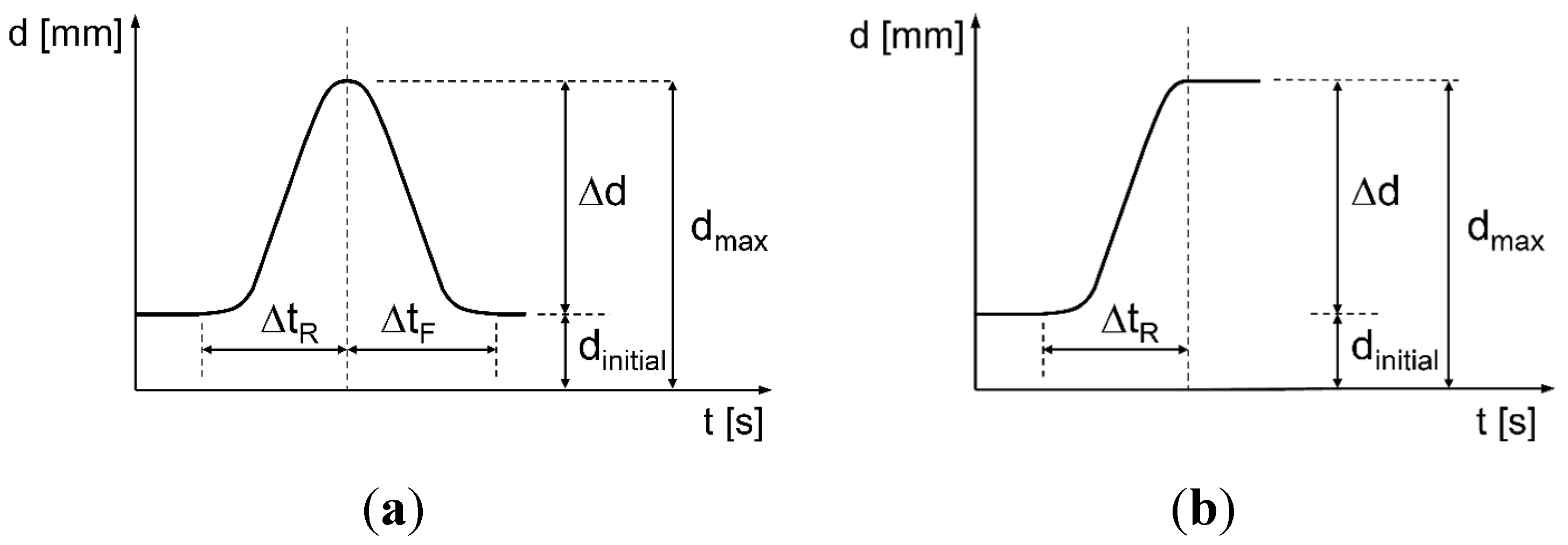Unsteady flow triggers processes like upwelling and downwelling, which govern the pressure gradient and pore water exchange in the hyporheic zone [2]. In experimental investigations of unsteady flow, hydrographs for both increasing and decreasing discharge typically follow a curve such as schematically presented in Figure 1a. Hysteresis effects are neglected in the present study. Symmetric hydrographs consist of a rising and a falling branch (Figure 1a), in contrary to a one-sided hydrograph that exclusively consists of one branch: in case of Figure 1b, a rising branch. Both hydrographs are characterized by the initial flow depth $d_{initial}$, maximum flow depth $d_{max}$, the total depth increase or decrease $\text{Δ}d=d_{max}-d_{initial}$ and the time duration for the rising branch $\text{Δ}{t}_R$ and falling branch $\text{Δ}{t}_F$. The ramping rates, $\text{Δ}d/\text{Δ}{t}_R$ and $\text{Δ}d/\text{Δ}{t}_F$, respectively, define the steepness of each branch. Graf and Suszka [1] introduced an unsteadiness parameter ${\Gamma }_{HG}$, which is used to combine the characteristics of a symmetric hydrograph in one factor:

$${\Gamma }_{HG}=\frac{1}{u_0^{*}}\frac{\text{Δ}d}{\text{Δ}t}$$

(1)

where $u_0^{*}=\sqrt{{\tau }_0/\rho }$ represents the shear velocity of the initial uniform flow condition, ${\tau }_0=\rho gd{S}_0$ the initial bed shear stress, $\rho$ the water density, $g$ the local gravitational acceleration, $d$ the flow depth and $S_0$ is the bed slope. Furthermore, $\text{Δ}t=\text{Δ}{t}_R+\text{Δ}{t}_F$ denotes the total duration of the rising and falling branch of the hydrograph. A high unsteadiness parameter implies therefore a rapid or very strong flow variation.

Figure 1. (a) Symmetric hydrograph; (b) One sided hydrograph.

Figure 1. (a) Symmetric hydrograph; (b) One sided hydrograph.

Song and Graf [3] performed an experimental study with unsteadiness parameters in the range of $0.0040<{\Gamma }_{HG}<0.0180$. They state that most of the analyzed hydrographs in their study did not show significant effects of unsteadiness compared to quasi-steady assumptions, both regarding the horizontal velocity profiles and turbulence intensity. Only for the largest unsteadiness parameters in the experimental range, they reported minor differences in the velocity profiles and turbulence intensities for the rising and falling branch.

Bed shear stress and lift are key factors when it comes to estimating the incipient motion of particles and therefore to evaluate the effect of the water flow on the riverbed. While shear stress is widely accepted to describe the threshold of particle motion, the influence of lift is often underestimated [4]. In fact, this has been a matter of debate over decades. Chepil [5] concludes that both lift and drag must be considered to describe the threshold of soil grain movement due to fluid motion. Chi-Hai [6] studied two thresholds for the incipient motion of particles: the rolling threshold and the lifting threshold, suggesting to apply both thresholds for sediment transport studies instead of using one combined “critical” parameter. This implies that lift should be regarded independently. More recently, Vollmer and Kleinhans [7] point out the importance of “vertical pressure gradients in the upper sediment layer”, which are directly connected to a certain lift force acting on the bed surface. Further studies investigate the pressure fluctuations in and above gravel beds and link their results to incipient motion of single particles [8,9]. In addition numerical investigations such as Derksen and Larsen [10] report strong lift forces, while others [11] still argue that lift forces can be neglected. While those studies are all based on steady flow, limited research has been performed to investigate the effect of unsteadiness in free surface flows. Some unsteady flow experiments focus on velocity measurements, sediment transport behavior or studied the river as an ecosystem [3,12,13,14,15,16,17]. Others address different types of flows, like gravity currents [18,19]. However, none addressed the direct influence of unsteadiness on bed shear stress and lift.

In the case of up- and downwelling, the pressure difference between surface water and ground water table causes surface water to infiltrate into the hyporheic zone or vice versa. Especially in armored gravel beds, where the armor layer has a porosity as low as 6% [20], the pressure gradient can be expected to be very high, resulting in a significant pressure difference from directly above to directly below the armor layer. The armor layer can be regarded as a kind of barrier between surface and subsurface water. Logically, this strong pressure gradient exerts a vertical stress or lift on the bed surface in up- or downward direction. Up- and downwelling are slow processes and can be explained from a hydrostatic perspective. Thus, they can be described as quasi-steady effects and contribute to the static lift on an armor layer. However, it is still to be investigated whether the unsteadiness of the surface flow above the armor layer accounts for an additional dynamic lift on the surface particles.

A direct measurement of shear stress and lift on a certain area of the riverbed is technically difficult because of its granular structure. In addition, granular bed surfaces, even in the form of static armor layers [21,22], are movable and therefore alter its surface arrangement over time. A single experiment rearranges the surface structure and changes the initial conditions for the subsequent experiment. Thus, the prerequisite conditions for a series of experiments are similar but not identical.

To overcome those problems, fixed beds or mixed forms of movable and fixed beds are reported in the literature. Previous studies partly included the use of pressure, drag or lift sensors [23,24,25,26]. A fixed or artificial streambed provides a persistent bed-surface structure for a series of experiments. 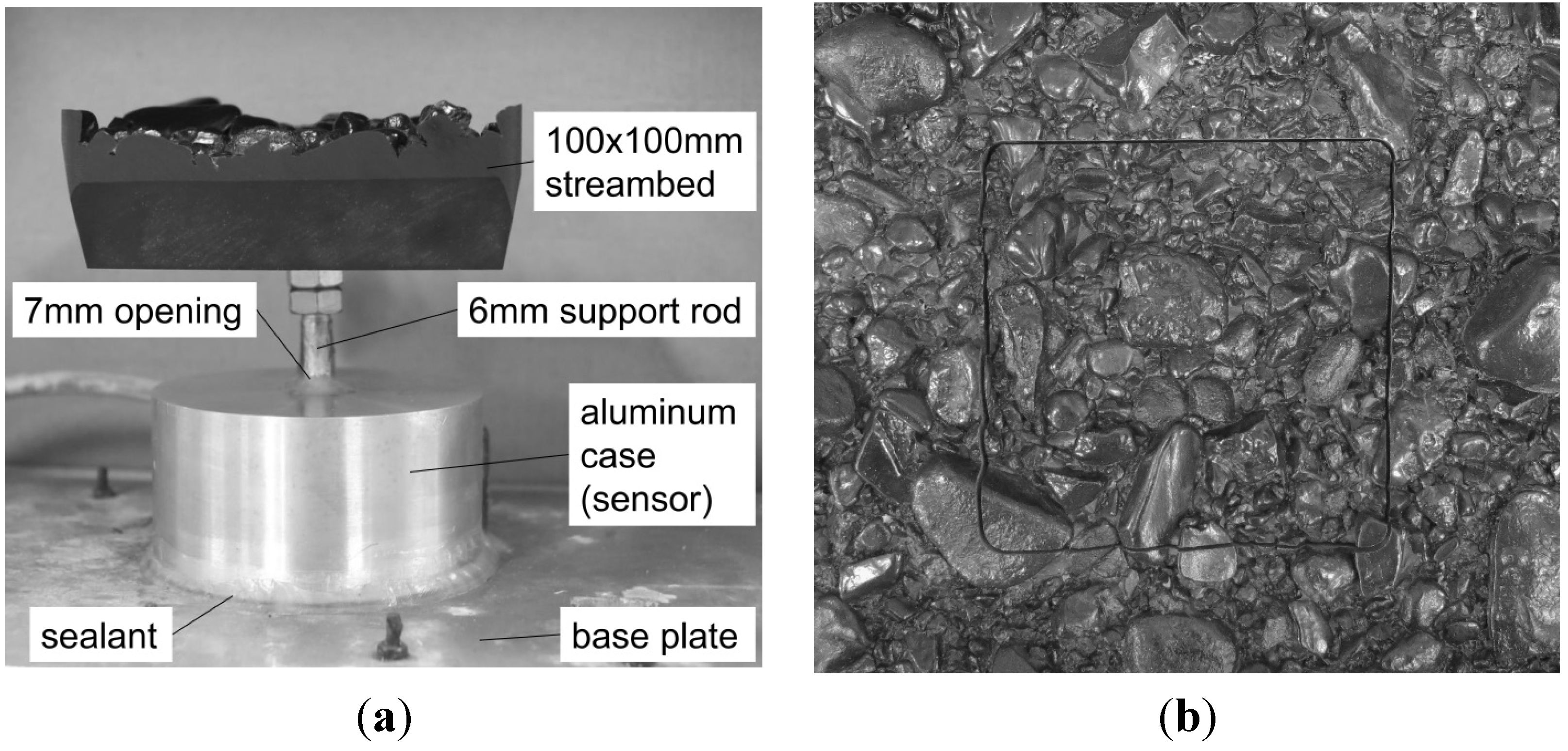Such beds often model a natural streambed artificially, with a well-defined, equally distributed roughness, using for example spherical obstacles [24]. The conditions for a series of experiments therefore represent an idealized model of a water-worked surface. To achieve a riverbed model closer to an original armor layer, Spiller et al. [27] present a technique to mold the surface structure of an actual gravel bed, which results in an artificial copy of a static armor layer. It models both exposed and hidden particles in great detail, including protruded surface grains and undercuts, and can produce multiple copies of the same surface structure. However, it does not model the subsurface porosity.

The present study provides results of direct lift measurements, using the aforementioned technique, for a large variety of flow variations. It focuses exclusively on increasing flow. Firstly, the experimental setup and all measurement devices are described in detail, followed by the experimental procedure. Secondly, the results of the experimental study are presented with focus on the influence of $\text{Δ}{t}_R$, $d_{initial}$, $\text{Δ}d$ and the armor layer porosity. Herewith, $\text{Δ}{t}_R$ is termed ramping duration. Thirdly, a discussion provides the perspective to link the experimental model to natural rivers. Finally, the key findings of this study are summarized in a conclusion.

2. Experimental Setup

2.1. Flume Setup

The experiments were carried out at the Fluid Mechanics Laboratory of the University of Auckland, New Zealand in an 19 m long, straight hydraulic flume with a width of w = 457 mm. A false floor, 125 mm above the original flume bed was installed on a length of 13.47 m (Figure 2). On this elevated part of the flume, an artificial streambed, described in detail further below, was installed on a length of 4.55 m and width of 0.391 m. Along each side of the artificial streambed, the remaining gap of 33 mm was closed by smooth PVC bars, in which six 10 mm diameter holes were drilled for de-aeration purposes. 1.80 m upstream and Then, 1.80 m downstream of the test section, the roughness of the flume base was adjusted to match the approximate roughness of the artificial streambed by fixing a layer of 20 mm to 30 mm diameter pebbles to the surface. The flume was glass sided along the entire length. Influences from the side walls were neglected.

Figure 2. Experiment setup. Longitudinal section. Not to scale.

Figure 2. Experiment setup. Longitudinal section. Not to scale.

Water was supplied to the flume through a single inflow pipe from a high reservoir with a constant head. A flow equalizer at the upstream end reduced the initial turbulence and assured a smooth water level close to the inlet. During steady flow conditions, the flow along the test section was uniform. A sharp crested weir was installed at the downstream end of the flume. The crest height was fixed at the elevation of the roughness tops in the channel at 160 mm above the original flume bed (Figure 2). The channel was long and rough enough that a fixed weir was sufficient to develop uniform flow without adjusting the downstream weir for each discharge. The bed slope was adjusted to 5‰.

To produce unsteady flow conditions during the experiments, an electric motor throttled a butterfly valve in the supply pipe. The motor speed and number of actuator turns were adjusted to produce the desired flow increase in a set amount of time, resulting in a linear increase in water supply.

2.2. Artificial Streambed

For the present study, the artificial streambed consists of a polyurethane cast, molded from an actual static armor layer. A two-component silicone rubber served as molding material providing a flexible form to cast the rigid streambed copy, made of a two-component polyurethane mixture with a density of 1.05 g/cm³. Because of its low density, the artificial streambed was mounted to the flume bottom. The molding procedure and materials are thoroughly described in [27]. The original armor layer was developed in a straight, 300 mm wide, hydraulic flume at the Leichtweiß-Institute for Hydraulic Engineering and Water Resources in Braunschweig, Germany, under uniform flow conditions, with a constant discharge of 29.8 L/s and a bed slope of 5‰. The surface grain size distribution, obtained by photographic line-by-number-analysis [28], was characterized by a mean grain diameter D_m = 13.5 mm, a D₅₀ = 11.4 mm and a maximum grain size of 32.0 mm with a coefficient of uniformity C_u = D₆₀/D₁₀ = 3.25. Of this original streambed (Figure 3a), a total area of 1.60 m in streamwise direction and 200 mm across, was molded and then reproduced (Figure 3b). Several reproductions provided enough material to cover the flume for the present study.

Figure 3. (a) Detail of the original armor layer; (b) Detail of the artificial streambed.

Figure 3. (a) Detail of the original armor layer; (b) Detail of the artificial streambed.

While the artificial streambed models the surface structure of the original bed in great detail, it does not reproduce the porous subsurface of a real gravel bed (Figure 4). For the last part of the present study, to allow representation of a porous subsurface with the artificial streambed, various numbers of 3 mm diameter holes were drilled into the artificial streambed. The holes were randomly distributed and preferably placed in gaps between exposed particles. The target piece (see Section 2.3) itself remained untouched, to preserve its shape or weight throughout all experiments. This allows rudimentarily simulating armor layer porosity and to study the influence of armor layer porosity on the observed unsteadiness effects. The identical experimental preconditions ensured that the same experiment could be performed several times, with an increasing number of holes. A larger number of holes in the artificial streambed increased the exchange of surface and subsurface water.

Figure 4. Model (a) vs. reality (b).

Figure 4. Model (a) vs. reality (b).

2.3. Force and Flow Depth Measurement

The vertical force on a 100 mm by 100 mm piece of the artificial streambed, indicating a certain lift at the streambed, was recorded during each experiment. A JR3 load cell, with a sensitivity of 0.00196 N (0.2 g) [24], allowed sampling at 1000 Hz. Figure 5a shows a side view of that section of the streambed, herewith termed target piece, mounted on the supporting rod of the sensor. The load cell was installed on an aluminum base plate and covered by an aluminum case. Only a 6 mm supporting rod penetrated the sensor case through a 7 mm opening. Petroleum jelly (Shell Snow White Petrolatum) was used to seal the gap between supporting rod and sensor case. This type of sealing material was shown to have negligible influence on the results [24]. Before the experiments, the sensor was tested under water, using several weights between 2 g and 300 g. To install the sensor and target piece at its appropriate position in the flume, a 102 mm by 102 mm hole was machined into the artificial riverbed. Since the target piece was cut from a duplicate of the original armor layer, it fitted perfectly into the adjoining artificial streambed structure, leaving a 1 mm gap along the edges (Figure 5b). The exact position of the target piece within the streambed was carefully chosen, to achieve an optimal representation of the entire streambed. Thus, general conclusions may be drawn based on the measured data. Three criteria were defined to choose the position of the target piece: (a) it was located in the centerline of the flume; (b) it was located in an area with only a few overly protruding particles; and (c) it had an approximately average distribution of particle sizes compared to the rest of the streambed. Although the flume was cleaned and the gap between target piece and streambed was regularly checked to be free of any blockage, a slight bevel along the lower edges of the target piece prevented any remaining dirt and sand grains from getting trapped. The load cell was connected by cable to its external electronics (spare board) and power supply outside the flume. From there, all data were transferred to a National Instruments connector block (CB-68LPR) and further to the PC.

A laser displacement sensor (Keyence LK-501) measured the water level above the center of the target piece synchronous to the force measurement (1000 Hz). The laser was mounted above the flume, pointing downwards. A very thin piece of plastic foil (ca. 50 mm × 100 mm) constantly floated on the water surface, providing a target surface for the laser beam (Figure 2).

Figure 5. (a) Target piece on sensor; (b) Target piece in position.

Figure 5. (a) Target piece on sensor; (b) Target piece in position.

2.4. Experimental Procedure

Each experiment was started at steady flow conditions. Two minutes into the experiment the motor was triggered to open the inflow valve, producing a one sided hydrograph (Figure 1b). Depending on the ramping rate and amount of flow increase, this phase took between 3 s and 120 s. Data recording continued to capture the final steady flow conditions for a total of eight minutes of experimental time.

To compare different hydrographs and to quantify their unsteadiness, the unsteadiness parameter for symmetric hydrographs ${\Gamma }_{HG}$ (Equation (1)) was utilized. The time duration of a one-sided hydrograph is approximately half as long as for the symmetric hydrograph. This approximation is in agreement with the data in [3] where the time duration of the rising and falling branch are mostly very similar ($\text{Δ}{t}_R\cong \text{Δ}{t}_F$). The following definition of ${\Gamma }_{HG}^{\prime }$ as an adjusted unsteadiness parameter made the results of one-sided hydrographs of the present study directly comparable to the symmetric data sets in the literature:

$${\Gamma }_{HG}^{\prime }=\frac{1}{u_0^{*}}\frac{\text{Δ}d}{2\text{·Δ}{t}_R}$$

(2)

Table 1 provides an overview of the range of hydrograph parameters covered by the present study, where $\text{Δ}Q$ denotes the total discharge increase in a hydrograph and $\text{Δ}Q/\text{Δ}{t}_R$ the ramping rate for the discharge increase at the test section. In total, 122 runs with 98 different hydrographs were performed on the non-porous bed and an additional 68 runs with an identical hydrograph were performed for 18 different bed-porosities.

Table 1. Experimental range of hydrograph parameters.

Parameter	Range
$\text{Δ}Q$	4.8 L/s–62.0 L/s
$\text{Δ}Q/\text{Δ}{t}_R$	0.56 L/s2–1.39 L/s2
$\text{Δ}d$	25 mm–129 mm
$d_{initial}$	20 mm–130 mm
$d_{max}$	67 mm–165 mm
${\Gamma }_{HG}^{\prime }$	0.0048–0.0800
Number of holes	0–1500
Bed porosity	0%–6.6%

Table 1. Experimental range of hydrograph parameters.

Parameter	Range
$\text{Δ}Q$	4.8 L/s–62.0 L/s
$\text{Δ}Q/\text{Δ}{t}_R$	0.56 L/s2–1.39 L/s2
$\text{Δ}d$	25 mm–129 mm
$d_{initial}$	20 mm–130 mm
$d_{max}$	67 mm–165 mm
${\Gamma }_{HG}^{\prime }$	0.0048–0.0800
Number of holes	0–1500
Bed porosity	0%–6.6%

3. Results

3.1. Water Level during Unsteady Flow

Figure 6 exemplarily presents the results for three similar flow increases, with different ramping durations. Figure 6a displays the water level over time for a flow increase with an unsteadiness parameter of ${\Gamma }_{HG}^{\prime }=0.013$, Figure 6b shows a similar graph for a higher unsteadiness parameter of ${\Gamma }_{HG}^{\prime }=0.021$ and Figure 6c represents an unsteadiness parameter of ${\Gamma }_{HG}^{\prime }=0.030$. For the subsequent analysis, the beginning of the unsteady part in each hydrograph was defined as the moment when the water level exceeded the initial mean value by more than ten times its standard deviation. As the water moves through the channel, the hydrograph is typically deformed compared to the flow increase at the supply pipe. Song and Graf [3] also observed this behavior, and Chow [29] explains it as follows: Increasing the discharge in a frictionless prismatic channel will result in uniformly progressive flow, where a stable wave profile propagates through the channel without changing its shape. In a rough channel, however, the shape of the wave is gradually altered by the effects of friction. For example, the wavefront of the hydrograph in Figure 6b,e was recorded at the test section with a delay of about 13 s after the flow increase at the inflow pipe was initiated. From there, the water level increased to 95% of its final value within 31 s and took another 8 s to complete the remaining 5%. In the following, the expression “hydrograph” always denotes the flow variation at the test section, such as presented in Figure 6. Furthermore, the propagating flow increase formed a monoclinal rising wave for low unsteadiness parameters (Figure 6a,d) and a steep wavefront for high unsteadiness parameters (Figure 6c,f). This is in agreement with Chow’s [29] observations of the wave profile during gradually and rapidly unsteady flow.

Figure 6. Water level above roughness tops and measured total lift over time during flow increase at three different ramping rates. d_initial = 57 mm, d_max = 128 mm, (a,d) Δt_R = 49.8 s; ${\Gamma }_{HG}^{\prime }$ = 0.013; (b,e) Δt_R = 30.8 s; ${\Gamma }_{HG}^{\prime }$ = 0.021; (c,f) Δt_R = 22.0 s; ${\Gamma }_{HG}^{\prime }$ = 0.030.

Figure 6. Water level above roughness tops and measured total lift over time during flow increase at three different ramping rates. d_initial = 57 mm, d_max = 128 mm, (a,d) Δt_R = 49.8 s; ${\Gamma }_{HG}^{\prime }$ = 0.013; (b,e) Δt_R = 30.8 s; ${\Gamma }_{HG}^{\prime }$ = 0.021; (c,f) Δt_R = 22.0 s; ${\Gamma }_{HG}^{\prime }$ = 0.030.

Until reaching 95% of the final water level, the hydrographs of most experimental runs resembled the form of a one-sided bell curve similar to Figure 1b. Within this range, significant effects of unsteady flow regarding the measured lift could be discovered and are discussed later on in this paper. However, any of these effects vanished after the water level reached this 95% mark. The remaining 5% are stretched over a substantially longer amount of time and observed behaviors can be explained from a quasi-steady perspective. Hence, for the calculation of the unsteadiness parameter, the 95% mark was regarded as the end of the unsteady part. Both beginning and end of the unsteady part are marked with a vertical dashed line in Figure 6a–f.

3.2. Lift during Unsteady Flow

The earlier described load cell directly measures the vertical force or lift force on the target piece. To obtain the lift ${\sigma }_{z\left(total\right)}$ in the unit of a vertical stress [N/m²] on the streambed, the lift force was divided by the target piece area (100 mm × 100 mm). A positive value of ${\sigma }_{z\left(total\right)}$ indicates the total lift on the target piece pointing in the upward direction. The directly measured or total lift ${\sigma }_{z\left(total\right)}$ is the sum of static lift ${\sigma }_{z\left(static\right)}$ representing the average lift during steady or quasi-steady flow and dynamic lift ${\sigma }_{z\left(dyn\right)}$, which covers eventual deviations from the static lift, yielding:

$${\sigma }_{z\left(total\right)}={\sigma }_{z\left(static\right)}+{\sigma }_{z\left(dyn\right)}$$

(3)

The lower diagrams in Figure 6 show the measured lift for the three example hydrographs. The beginning and end (95%) of the unsteady period within each experiment is again marked by vertical dashed lines. In the very beginning and very end of each experiment, the flow was steady and uniform. In general, slightly negative lift was observed during steady flow. This is in contrary to Einstein and El-Samni [4], who generally observed positive lift during steady flow, which is addressed in Section 4.3 below. With higher discharges, stronger negative lift was measured.

Looking at a moderate flow increase with an unsteadiness parameter of ${\Gamma }_{HG}^{\prime }=0.013$ (Figure 6a,d), the measured lift gently drifted from its initial steady value to the final steady value, accordingly from a negative lift of approximately 16 N/m² to a negative lift of approximately 40 N/m². We call this steady level of lift, which is unique for each discharge, “steady lift”. In between, i.e., in the unsteady period of the experiment, the measured lift followed a linear trend over time. Such a linear connection of the initial and final level was regarded as quasi-steady and the dynamic part of the lift ${\sigma }_{z\left(dyn\right)}$ was negligible. Thus, Figure 6a,d marks the trend of the static lift during a flow increase. Therefore, a linear trend line such as in Figure 6a,d was constructed similarly for all other experiments, as a reference for the static lift component ${\sigma }_{z\left(static\right)}$.This quasi-steady reference appears as a thin grey line in Figure 6a,d. Any major deviation from this reference line was considered a significant dynamic lift force ${\sigma }_{z\left(dyn\right)}$ and regarded as an unsteady effect.

With an increasing unsteadiness parameter, the dynamic lift indicated significant peaks. Figure 6c,f shows how the ${\sigma }_{z\left(total\right)}$ deviates from the quasi-steady reference line, indicating dynamic lift. In all experiments with an unsteadiness parameter of ${\Gamma }_{HG}^{\prime }>0.02$, three major peaks were recorded: Shortly before the approaching front wave of the flow increase reached the target piece, it caused a positive dynamic lift (Peak 1). Once the front wave actually reaches the test section, the dynamic lift inverts to a strong negative value (Peak 2), followed by a continuous flow increase, where ${\sigma }_{z\left(total\right)}$ increased again and eventually showed another positive dynamic lift (Peak 3). With the end of the unsteady period, ${\sigma }_{z\left(total\right)}$ matches the quasi-steady reference line. This last peak was generally longer lasting than the first two. To emphasize the three peaks in Figure 6, the area between the quasi-steady reference line and the measured ${\sigma }_{z\left(total\right)}$ is shaded in grey. The circles mark the point of maximum deviation from the quasi-steady reference line for each of the three peaks. All further analyses in the present study are based on these local extrema of the dynamic lift ${\sigma }_{z\left(dyn\right)}$.

Figure 7 shows for all three peaks that the maximum dynamic lift increased with the unsteadiness parameter. The grey shaded area in Figure 7 marks the range of unsteadiness parameters covered in [3].

Three parameters determine the unsteadiness parameter: $\text{Δ}{t}_R$ (in form of the ramping rate $\text{Δ}d/\text{Δ}{t}_R$), $d_{initial}$ (in form of $u_0^{*}$) and $\text{Δ}d$ (at a constant ramping rate). By keeping two of those parameters constant, the influence of the remaining one can be isolated and analyzed independently. The following sections present the influence of each of those three parameters on the observed lift peaks during unsteady flow.

Figure 7. Dynamic lift for Peak 1 (a), Peak 2 (b), and Peak 3 (c), plotted with trend lines over the hydrographs unsteadiness parameter. The grey area covers the range of unsteadiness parameters addressed in [3] ( $0.004<{\Gamma }_{HG}<0.018$).

Figure 7. Dynamic lift for Peak 1 (a), Peak 2 (b), and Peak 3 (c), plotted with trend lines over the hydrographs unsteadiness parameter. The grey area covers the range of unsteadiness parameters addressed in [3] ( $0.004<{\Gamma }_{HG}<0.018$).

3.3. Influence of the Ramping Rate

As shown in Figure 6, a similar flow increase, but taken place over various ramping durations $\text{Δ}{t}_R$, alters the magnitude of the dynamic lift peaks. In fact, the shorter the time difference between the beginning and end of the flow variation, the higher the dynamic lift. Hence, for constant initial and final flow depths, changes in $\text{Δ}{t}_R$ are responsible for variations in $\text{Δ}d/\text{Δ}{t}_R$, which are qualitatively comparable to the ramping rate $\text{Δ}Q/\text{Δ}{t}_R$.

A small $\text{Δ}{t}_R$ value conforms to a high unsteadiness parameter (Equation (2)) and therefore accounts for stronger unsteady effects (Figure 7). To draw conclusions about the influence of $\text{Δ}{t}_R$ for various hydrograph conditions, Figure 8 presents the maximum dynamic lift for each peak for 85 experimental runs, covering the entire spectrum of $\text{Δ}Q/\text{Δ}{t}_R$ and $d_{initial}$ (Table 1) for two different $\text{Δ}Q$. Figure 8a shows how Peak 1 develops for a fixed flow increase of $\text{Δ}Q=28.6L/s$ under six different ramping rates $\text{Δ}Q/\text{Δ}{t}_R$ and therefore different $\text{Δ}{t}_R$ values. It can be seen that, apart from very few outliers, the highest ramping rates cause the strongest dynamic lift peaks. With increasing $d_{initial}$, this trend diminishes. Figure 8d shows the same trend and the same magnitudes of ${\sigma }_{z\left(dyn\right)}$ for a flow increase of $\text{Δ}Q=57.2L/s$. Both, the flow and ramping duration are doubled, resulting in the same ramping rate. Note that the $\text{Δ}Q=57.2L/s$ runs could not be performed with higher initial flow depths than 66 mm because of a limited flume capacity. Furthermore, the highest ramping rate was only applied to the $\text{Δ}Q=28.6L/s$ runs.

Figure 8b,e displays a similar result for Peak 2. Again, the highest ramping rates achieve the strongest dynamic lift peak, independent of the initial flow depth and both $\text{Δ}Q=28.6L/s$ and $\text{Δ}Q=57.2L/s$ show equal results for the same ramping rates.

On the contrary, Peak 3 does not show significant trends for $\text{Δ}Q=28.6L/s$ (Figure 8c) but a substantial dynamic lift for $\text{Δ}Q=57.2L/s$ (Figure 8f). In that case again, high ramping rates caused strong forces.

Figure 8. Dynamic lift for each peak and for different ramping rates plotted with trend lines over the initial flow depth of each experiment. Each for two different flow increases: (a–c) $\text{Δ}Q=28.6L/s$ and (d–f) $\text{Δ}Q=57.2L/s$. A higher ΔQ corresponds to a higher Δd, but Δd for each experimental run is dependent on $d_{initial}$.

Figure 8. Dynamic lift for each peak and for different ramping rates plotted with trend lines over the initial flow depth of each experiment. Each for two different flow increases: (a–c) $\text{Δ}Q=28.6L/s$ and (d–f) $\text{Δ}Q=57.2L/s$. A higher ΔQ corresponds to a higher Δd, but Δd for each experimental run is dependent on $d_{initial}$.

3.4. Influence of the Initial Water Level

Figure 8 also shows the influence of the initial water level on the observed dynamic lift. For all three peaks and all presented $\text{Δ}Q$, the measured ${\sigma }_{z\left(dyn\right)}$ generally decreased with increasing initial flow depth. For very high initial flow depths, unsteady effects almost vanished completely and the ${\sigma }_{z\left(dyn\right)}$ readings converge to 0.

However, the measured value of ${\sigma }_{z\left(dyn\right)}$ never actually reached 0 because turbulent fluctuations in the static lift force always cause minor deviations from the static reference line (Figure 6d). The higher the discharge is, and therefore the flow depth, the stronger the turbulent fluctuations become. Thus, very low ramping rates, where the dynamic lift can also be expected to be negligible, even indicate a slightly increasing trend with increasing initial flow depth (Figure 8a,b).

The two highest ramping rates caused a clear front wave at the tip of the hydrograph (Figure 6c), while lower ramping rates were characterized by a gradually depth increase over time (Figure 6a). Interestingly, those high ramping rates, combined with low initial flow depths, did not follow the regular trend in peak 1 (Figure 8a). The lowest initial flow depth, in combination with the highest ramping rates, did not show the strongest dynamic lift and a higher order trend had to be applied to characterize the resulting curve.

3.5. Influence of the Hydrograph’s Total Depth Increase

To isolate the influence of the flow depth increase $\text{Δ}d$ from the other hydrograph characteristics, a series of 13 experimental runs was performed. The initial flow depth for each run was set to 42 mm above the roughness tops, which corresponds to a discharge of 6.5 L/s. Changing just $\text{Δ}d$, and leaving $\text{Δ}{t}_R$ constant, would imply a change in ramping rate, so that the results would basically repeat the earlier described influence of $\text{Δ}{t}_R$ or $\text{Δ}Q/\text{Δ}{t}_R$. In this section, the ramping rate was kept constant to isolate the effect of $\text{Δ}d$ from the effect of the ramping rate. Thus, $\text{Δ}{t}_R$ was adjusted so that each flow increase featured the same ramping rate of $\text{Δ}Q/\text{Δ}{t}_R$ = 1.29 L/s².

Figure 9 shows the maximum dynamic lift for each of the three peaks depending on the change in flow depth. All three peaks show a higher ${\sigma }_{z\left(dyn\right)}$ for a higher $\text{Δ}d$. Peaks 1 and 2, which occur at the beginning of the flow increase, display a significant effect even for rather small flow increases. Above a certain degree of flow increase, however, these two first peaks do not show any additional activity and ${\sigma }_{z\left(dyn\right)}$ remains constant. Peak 2 is generally larger than Peak 1.

Figure 9. Dynamic lift for each peak, plotted with trend lines over change in flow depth. Initial flow depth and ramping rate kept constant at $d_{initial}$ = 42 mm and $\text{Δ}Q/\text{Δ}{t}_R=1.29L/s^2$. Markers: (+) Peak 1, (×) Peak 2, (○) Peak 3.

Figure 9. Dynamic lift for each peak, plotted with trend lines over change in flow depth. Initial flow depth and ramping rate kept constant at $d_{initial}$ = 42 mm and $\text{Δ}Q/\text{Δ}{t}_R=1.29L/s^2$. Markers: (+) Peak 1, (×) Peak 2, (○) Peak 3.

In contrast, Peak 3 seems rather insignificant for small flow increases but represents the largest of all three peaks for stronger flow increases. It maintains this trend until the upper end of the experimental spectrum.

Cases $\text{Δ}Q=28.6L/s$ and $\text{Δ}Q=57.2L/s$, presented in Figure 8, correspond to average depth increases of $\text{Δ}d=75mm$ and $\text{Δ}d=109mm$, respectively, depending on the initial flow depth. According to Figure 9, those flow increases have similar effects on Peak 1. Peak 2 is also comparable for both cases. This is in agreement with Figure 8, where the $\text{Δ}Q=28.6L/s$ and $\text{Δ}Q=57.2L/s$ runs show similar graphs for Peak 1 (Figure 8a,d), as well as Peak 2 (Figure 8b,e). However, Peak 3 is certainly much larger for a flow increase of $\text{Δ}d=109mm$, compared to $\text{Δ}d=75mm$ (Figure 9), which, again, is in agreement with the earlier mentioned difference of the $\text{Δ}Q=28.6l/s$ and $\text{Δ}Q=57.2L/s$ graphs in Figure 8c,f.

3.6. Influence of the Armor Layer Porosity

The porous structure of a gravel bed is very complex and cannot be mimicked by the artificial streambed used in this study. However, the artificial streambed can be modified to allow a pressure exchange between surface and ground water. In a real gravel bed, the pore water in the subsurface material is connected to the flowing water above the streambed through the porosity of the armor layer and subsurface material. Thus, the pore water pressure p₀ and the pressure above the gravel bed p₁ (Figure 4) can communicate. However, the artificial bed surface in this study was non-porous, so that p₀ and p₁ were basically disconnected. Only the gap around the target piece provided a small area for pressure equalization, which has been neglected in the porosity calculation below.

Using drilled holes to resemble porosity, it can be seen that armor layer porosity had a major effect on the dynamic lift peaks. Figure 10a shows how an increasing number of holes in the artificial bed significantly reduced the dynamic lift peaks. Beyond approximately 1000 holes, a further increase in porosity did not show any additional reduction. Even for 1500 holes, similar lift peaks, as observed for the non-porous bed, were clearly recognizable (Figure 10b).This bed modification was performed on an area of 400 mm by 400 mm around the target piece, while the target piece itself remained untouched. Even though this is not a direct equivalent of the porous structure in a real gravel bed, the number of holes can still be associated with a measurable porosity of the streambed. Each hole has a diameter of 3 mm, giving it a surface area of A_hole = 7.07 mm2. The total size of the modified area is $A_{total}$ = (400 mm)² = 160,000 mm². The average thickness of the artificial bed $h_{bed}$ and the average length of the holes can be regarded as equal, so that the combined volume of all holes $V_{holes}$ can be related to the total volume of the modified area $V_{total}$ within the artificial streambed to get some measure for the streambed porosity. A number of 1500 holes would then resemble the following porosity:

$$\text{Φ}=\frac{V_{holes}}{V_{total}}=\frac{1500·A_{hole}·h_{bed}}{A_{total}·h_{bed}}=6.6\%$$

(4)

Investigations have shown that real armor layers often have a porosity close to 6% [20]. The experiments with about 1000 to 1500 holes might therefore be a good comparison to a real armor layer. The dynamic lift peaks were clearly visible in the experiments’ results (see Figure 10).

Figure 10. Experiments over a modified, porous streambed with a constant hydrograph: $d_{initial}$ = 67 mm, $d_{max}$ = 132 mm, $\text{Δ}Q$ = 28.6 L/s, $\text{Δ}{t}_R$ = 21.8 L/s², ${\Gamma }_{HG}^{\prime }$ = 0.026. (a) Dynamic lift for each peak, plotted with trend lines over the number of holes drilled into the artificial streambed (hole diameter: 3 mm). Streambed porosity in % according to Equation (4); (b) Water level above roughness tops and total measured lift force over time during flow increase with a modified, highly porous bed (1500 holes).

Figure 10. Experiments over a modified, porous streambed with a constant hydrograph: $d_{initial}$ = 67 mm, $d_{max}$ = 132 mm, $\text{Δ}Q$ = 28.6 L/s, $\text{Δ}{t}_R$ = 21.8 L/s², ${\Gamma }_{HG}^{\prime }$ = 0.026. (a) Dynamic lift for each peak, plotted with trend lines over the number of holes drilled into the artificial streambed (hole diameter: 3 mm). Streambed porosity in % according to Equation (4); (b) Water level above roughness tops and total measured lift force over time during flow increase with a modified, highly porous bed (1500 holes).

4. Discussions

4.1. Model vs. Reality

The obtained data show a significant influence of single hydrograph characteristics on the dynamic lift. Two major simplifications were performed in the present study to model a natural gravel bed. The surface material, i.e., the static armor layer, was represented by a non-porous artificial streambed and the pore water, which is usually distributed within the granular structure of the subsurface material, was modeled by a non-moving, clear water body below the artificial streambed. This offers a unique opportunity to directly measure the total lift force on a streambed patch.

Figure 4 shows how the physical model of the present study compares to a real streambed. The model consists of a solid artificial armor layer, where the gap around the target piece is the only connection of surface and subsurface water in the vicinity of the sensor. However, a real armor layer is certainly a very close-grained structure, but still offers porosity. It therefore provides a well-distributed network of connections between surface and subsurface water. Hence, the pressure above the armor layer and the pore pressure in the subsurface material might communicate in a different way as they do in the model. Investigations [20] have shown that the porosity of armor layers is much smaller ($\text{Φ}=6\text{\%})$ compared to the subsurface material ($\text{Φ}=20\text{\%})$. The armor layer is comparable to an almost solid layer that divides the surface water from the underlying pore system, which is very close to the conditions in the model.

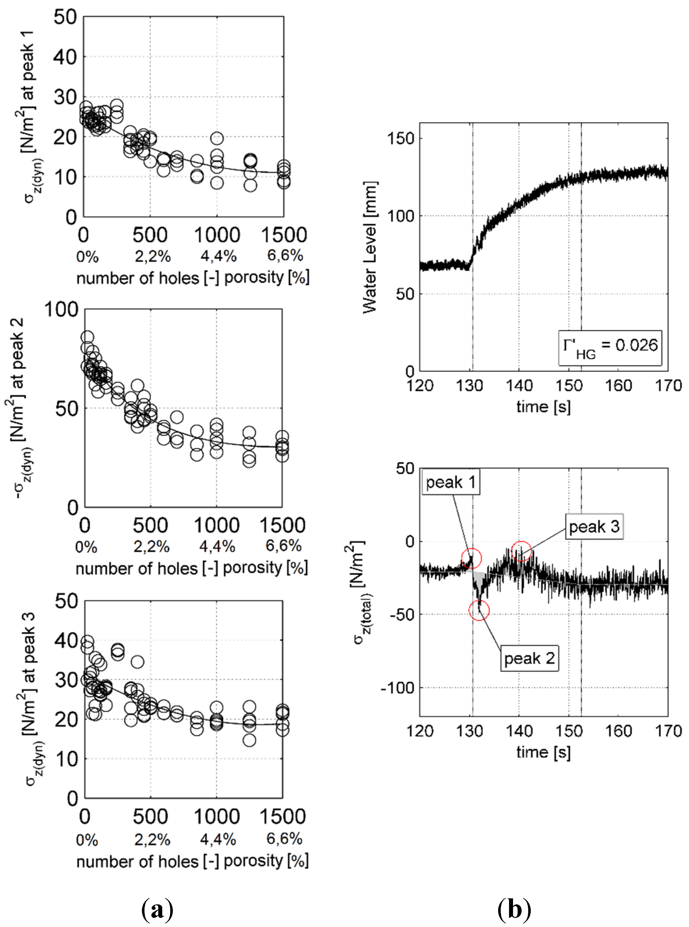
The present study further investigates the influence of the armor layer porosity by modifying the solid streambed and connecting the subsurface and surface water column via a number of randomly distributed holes. Accordingly, the natural armor layer porosity was underestimated by the solid bed (0 holes; $\text{Φ}=0\text{\%}$) and slightly overestimated by the most porous bed (1500 holes; $\text{Φ}$ = 6.6%). Both the upper and lower limit in porosity showed qualitatively similar results, so that comparable dynamic lift peaks can be expected in a natural gravel bed. Quantitatively however, expected ${\sigma }_{z\left(dyn\right)}$ values in a real armor layer might be estimated lower than the values from the solid bed results and slightly higher than the values of the most-porous bed results in this study.

It remains unclear whether the granular structure of real subsurface material implicates a general dampening or time lag of pressure exchanges between the surface- and subsurface water, compared to the clear water body in the model. It is, furthermore, uncertain what influence such a dampening would have on the observed dynamic lift peaks. An adjusted model, including a granular subsurface material below the porous streambed, might be applicable for future investigations regarding the influence of the subsurface material, which should also include pressure measurements above and below the armor layer.

4.2. Range of Unsteadiness Parameters

Unsteady flow in rivers has various origins such as natural floods, hydropower peaking or even dam break scenarios. The unsteadiness of the flow in such examples can range from mild flow variations, to very rapid fluctuations. To cover most of this variety, the present study included hydrographs with a wide range of unsteadiness parameters, $0.0048<{\Gamma }_{HG}^{\prime }<0.0800$. As a practical example: Recent field studies on hydropower peaking have shown that unsteadiness parameters of ${\Gamma }_{HG}^{\prime }=0.0180$ and higher, also occur in real gravel bed streams. Applying Equation (2) to the raw data of a field study at River Lundesokna in Norway [2], a hydrograph with an unsteadiness parameter of ${\Gamma }_{HG}^{\prime }=0.0183$ could be observed downstream a hydropower plant on 30 January 2012. In comparison, the largest unsteadiness parameter in the study of [3] is ${\Gamma }_{HG}=0.0180$, resulting in hardly recognizable significant unsteady effects for this measurement range (Figure 7). Song and Graf [3] used a slightly wider but comparable channel to the one in the present study. The maximum specific discharges used in both studies were also in a similar range. The present study, however, covered lower initial depths, as well as higher ramping rates.

4.3. Negative Lift during Steady Flow

During steady flow, negative lift was experienced in the present study. Einstein and El-Samni [4] stated the lift on a rough surface during steady open channel flow to be generally positive in upward direction. A possible explanation for the contrary observations in the present study could be the individual shape of the streambed in the target piece area. The target piece area was carefully chosen to represent the entire streambed in order to draw general conclusions (see Section 2.3). However, some areas of the riverbed are formed differently than others, so that the vertical stress on the bed is not equally distributed. Depending on the surface structure and the orientation in which single grains are exposed to the flow, it is only reasonable that some areas experience a slight lift. Others must be affected in the opposite way with a slight downward pressure. The integral of the vertical stress over a large area is still slightly positive in upward direction, according to [4].

In fact, Friedrich et al. [30] performed velocity measurements during steady flow over the exact same artificial surface as the present study. The measurements show that an exposed grain upstream the target piece causes a downward velocity component in the target piece area. This downward velocity exerts a downward force or negative lift on the target piece. Higher discharges cause higher downward velocities and therefore a higher negative static lift in this area.

For the present study, a neutral section of the streambed would be preferred for lift measurements, since the static lift would be negligible and the measured total lift would directly represent the dynamic lift. However, it is difficult to identify which part of the bed surface acts in that way. Even though the chosen segment for force measurements was representative for the entire streambed in terms of shape and grain size distribution, it turned out to be subject to a negative static lift force. This tendency increases with the discharge and is persistent throughout all experimental runs.

To adjust the results for general conclusions, the static lift was subtracted from the total lift by relating all lift peaks to a quasi-steady reference line. In a neutral section of the riverbed, where neither lift nor downward pressure occurs during steady flow, this reference line would be constant at ${\sigma }_{z\left(dyn\right)}$ = 0. Any significant deviation of the force measurement from this reference line was regarded as dynamic lift, or in other words, an unsteady effect that is not describable with a quasi-steady approach. Thus, the dynamic lift, which is the core parameter of this investigation, is regarded to be representative for the entire flume, so that general conclusions can be drawn from this investigation.

4.4. The Cause of the Dynamic Lift Peaks

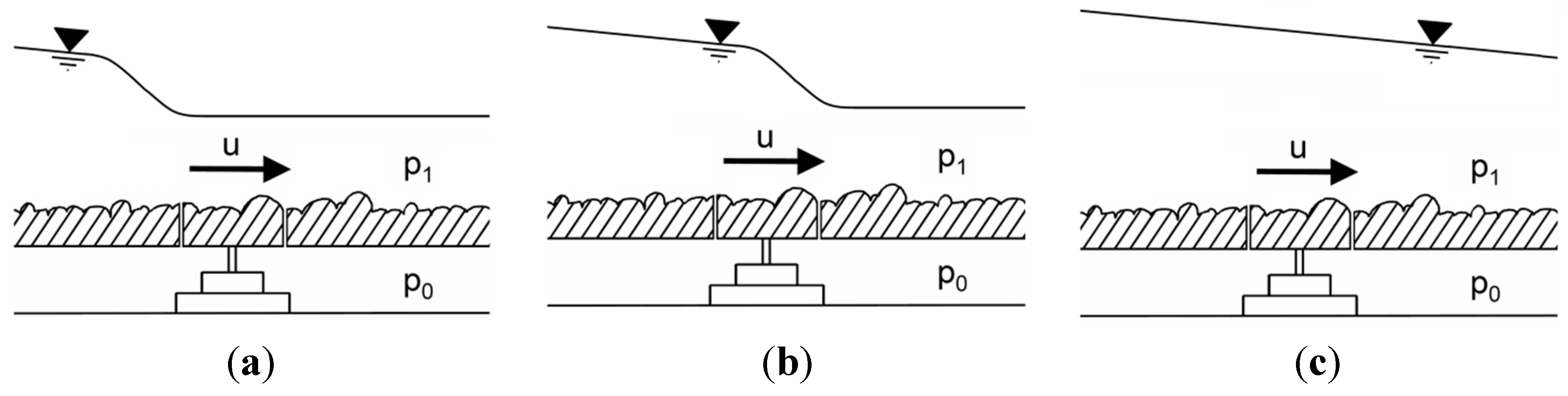
The first peak occurs a few seconds before the tip of the increasing water flow reaches the target piece. Figure 11a shows the water level during Peak 1. A rather steep depth increase is approaching the test section. The main part of the measured lift in this case results from a pressure difference below and above the bed surface, p₀ and p₁, respectively. Peak 1 corresponds to a positive dynamic lift in upward direction, p₀ must therefore be larger than p₁. Assuming hydrostatic pressure above the target piece, p₁ correlates with the initial flow depth. On the other hand, below the target piece, p₀ seems to be partly influenced by the elevated flow depth further upstream. Through small gaps at the upstream end of the artificial bed as well as through the de-aeration holes in the PVC bars besides the artificial bed, p₀ could already build up to an increased level before the free surface wave above the bed reached the target piece. Hence, the target piece experiences a positive dynamic lift. In an actual riverbed, this translates to a situation where through a breach in the clogged armor layer, pressure builds up in the porous subsurface material and causes lift on the armor layer further downstream.

The beginning of the second peak coincides with the rather steep wave front arriving at the target piece (Figure 11b). At a certain moment, the hydrostatic pressure above the bed surface increases significantly. At this stage, the subsurface pressure still depends partly on the increased pressure from upstream and the initial pressure from downstream, so that p₁ even exceeds p₀ for a moment causing negative lift. Peak 2 ends after a few seconds when p₀ adjusts to p₁.

Figure 11. Schematic water level above the test section during the occurrence of the dynamic lift peaks: (a) Peak 1; (b) Peak 2; and (c) Peak 3.

Figure 11. Schematic water level above the test section during the occurrence of the dynamic lift peaks: (a) Peak 1; (b) Peak 2; and (c) Peak 3.

The steep tip of the approaching flow increase is followed by a consistent increase in flow depth, lasting for a much longer time than Peaks 1 and 2. In a similar way to Peak 1, p₀ is possibly affected by the further depth increase approaching from upstream and causes positive dynamic lift, i.e., Peak 3. Depending on the water surface slope, which directly correlates to the ramping rate, a larger difference between p₀ and p₁ could be expected. 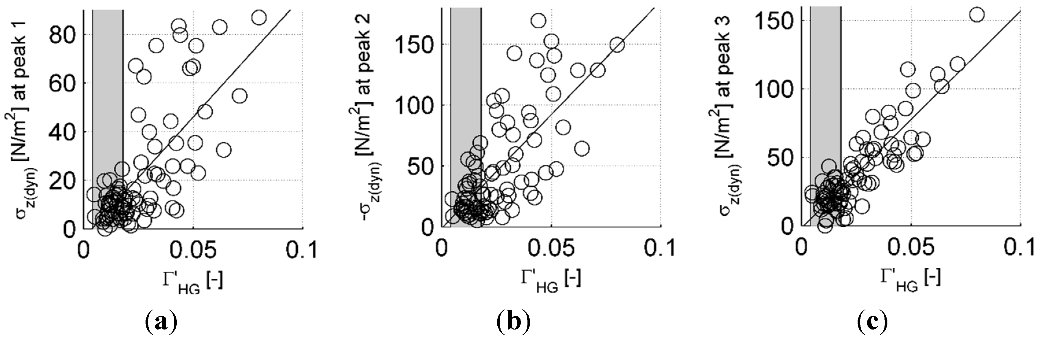This explains why higher ramping rates lead to larger dynamic lift in Peak 3 (Figure 6). 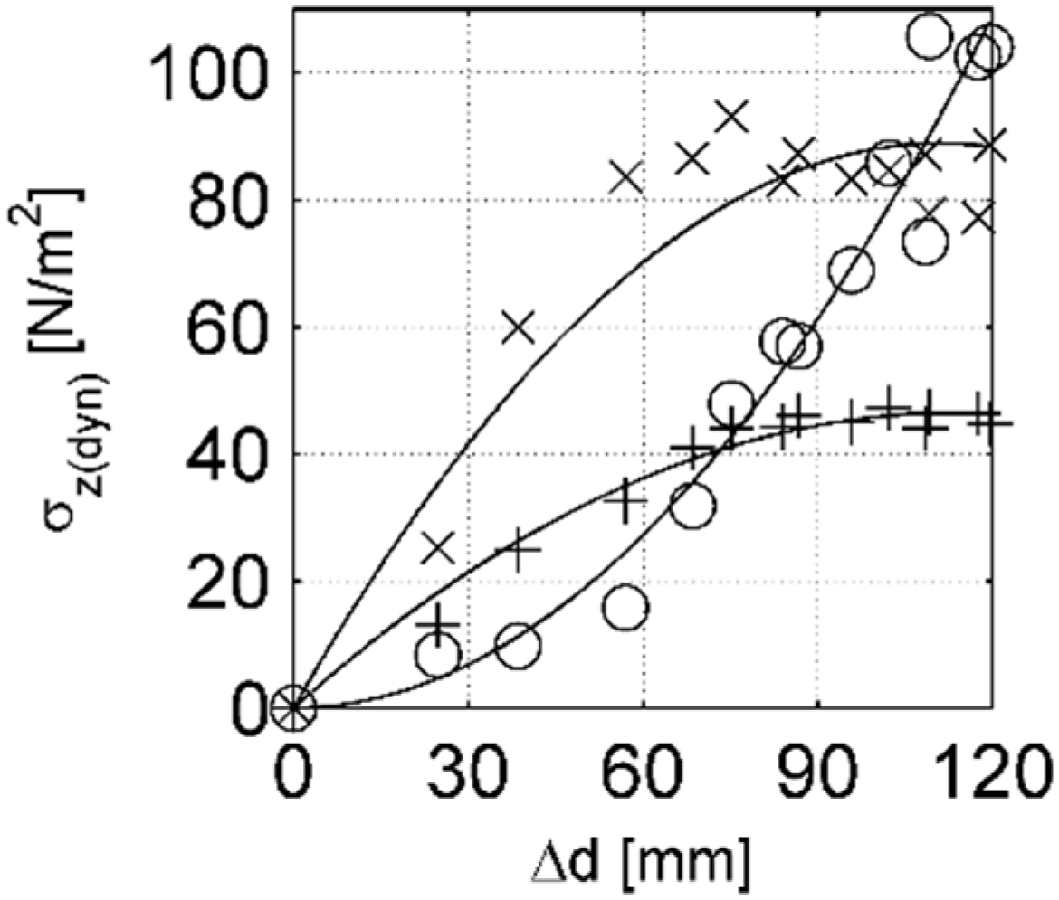It does not explain why stronger dynamic lift was recorded for higher $\text{Δ}d$ values, with a constant ramping rate (Figure 9). It seems that additional, hydrodynamic effects enhance the dynamic lift in Peak 3. Investigations regarding the velocity field above the streambed during unsteady flow are suggested to provide further conclusions.

5. Conclusions

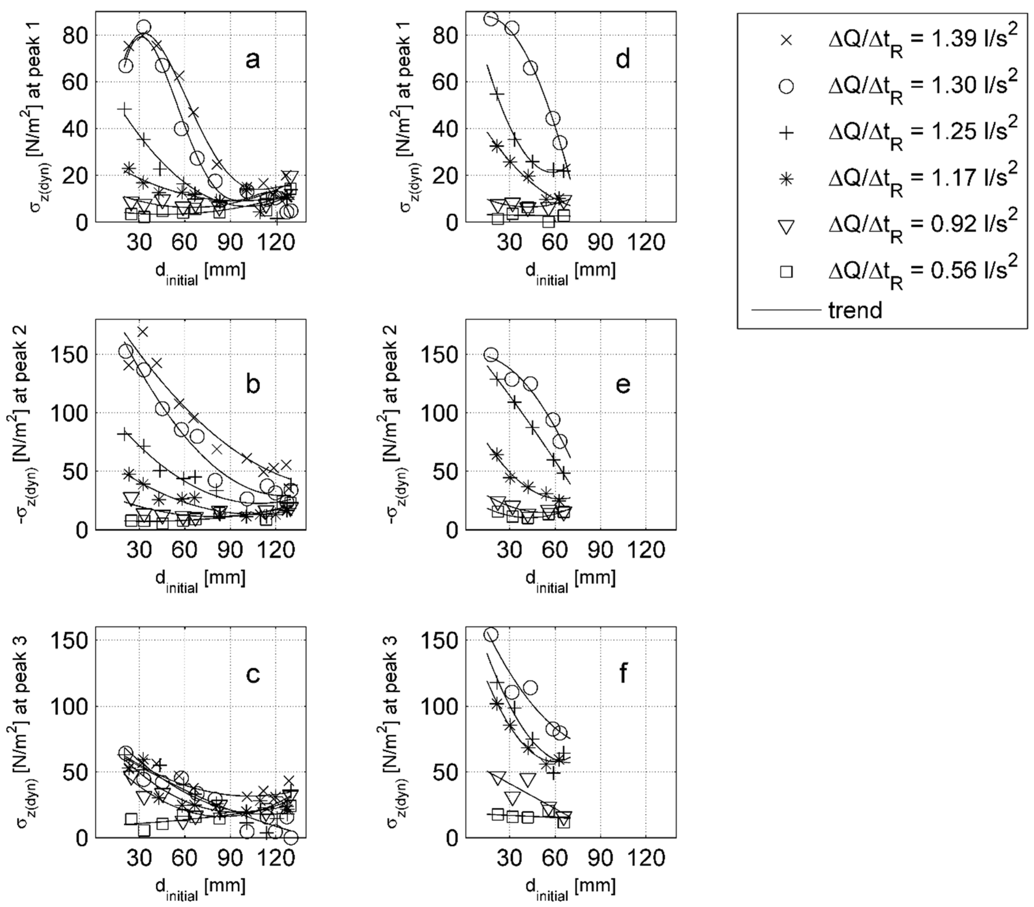
The lift on a 100 mm × 100 mm piece of artificial streambed was directly measured during unsteady flow in a physical experiment. Increasing the flow from a lower to a higher discharge, a wide spectrum of unsteadiness parameters and porosities was tested during 190 experimental runs. In general, three major dynamic lift peaks were recorded for experiments with unsteadiness parameters of ${\Gamma }_{HG}^{\prime }>0.02$. Comparing the maximum dynamic lift during the observed peaks, the influence of single hydrograph characteristics could be isolated and evaluated. Initial flow depth, duration and extent of the flow increase are therefore the key factors influencing dynamic lift during highly unsteady flow.

The observed unsteady effects in form of dynamic lift peaks were increasing with: (1) decreasing initial flow depth $d_{initial}$; (2) increasing ramping rate $\text{Δ}d/\text{Δ}{t}_R$ and therefore decreasing ramping duration $\text{Δ}{t}_R$; (3) increasing flow variation $\text{Δ}d$ or $\text{Δ}Q$ at a constant ramping rate, especially regarding Peak 3; and, finally, (4) increasing unsteadiness parameter ${\Gamma }_{HG}^{\prime }$.

Additional experiments showed a major influence of the armor layer porosity on the observed dynamic lift peaks. Increasing armor layer porosity reduced the dynamic lift, but could not make it disappear entirely.

The present study shows that lift, which is compared to the shear stress and is often neglected during steady flow, plays a vital role in the interaction between unsteady flow and the streambed.

References

1. Graf, W.H.; Suszka, L. Unsteady Flow and Its Effect on Sediment Transport. In Proceedings of International Association for Hydraulic Research (IAHR) Preprinted Proceedings: 21st Congress, Melbourne, Australia, 19–23 August 1985; pp. 85–13.
2. Casas-Mulet, R.; Alfredsen, K.; Hamududu, B.; Timalsina, N.P. The effects of hydropeaking on hyporheic interactions based on field experiments. Hydrol. Process. 2014, 29, 1370–1384. [Google Scholar] [CrossRef]
3. Song, T.; Graf, W.H. Velocity and turbulence distribution in unsteady open-channel flows. J. Hydraul. Eng. 1996, 122, 141–154. [Google Scholar] [CrossRef]
4. Einstein, H.A.; El-Samni, E.S.A. Hydrodynamic forces on a rough wall. Rev. Mod. Phys. 1949, 21, 520–524. [Google Scholar] [CrossRef]
5. Chepil, W.S. The use of evenly spaced hemispheres to evaluate aerodynamic forces on a soil surface. Trans. Am. Geophys. Union 1958, 39, 397–404. [Google Scholar] [CrossRef]
6. Chi-Hai, L. Criteria for incipient motion of spherical sediment particles. J. Hydraul. Eng. 1995, 121, 472–478. [Google Scholar]
7. Vollmer, S.; Kleinhans, M.G. Predicting incipient motion, including the effect of turbulent pressure fluctuations in the bed. Water Resour. Res. 2007, 43. [Google Scholar] [CrossRef]
8. Detert, M.; Weitbrecht, V.; Jirka, G.H. Laboratory measurements on turbulent pressure fluctuations in and above gravel beds. J. Hydraul. Eng. 2010, 136, 779–789. [Google Scholar] [CrossRef]
9. Hofland, B.; Battjes, J.; Booij, R. Measurement of fluctuating pressures on coarse bed material. J. Hydraul. Eng. 2005, 131, 770–781. [Google Scholar] [CrossRef]
10. Derksen, J.J.; Larsen, R.A. Drag and lift forces on random assemblies of wall-attached spheres in low-Reynolds-number shear flow. J. Fluid Mech. 2011, 673, 548–573. [Google Scholar] [CrossRef]
11. Hong, A.; Tao, M.; Kudrolli, A. Onset of erosion of a granular bed in a channel driven by fluid flow. Phys. Fluids 2015, 27. [Google Scholar] [CrossRef]
12. Bagherimiyab, F.; Lemmin, U. Sediment flux dynamics in turbulent unsteady open-channel flow over a gravel bed. Environ. Hydraul. 2010, 2, 783–788. [Google Scholar]
13. Bombar, G.; Elçei, Ş.; Tayfur, G.; Göney, M.Ş.; Bor, A. Experimental and numerical investigation of bed-load transport under unsteady flows. J. Hydraul. Eng. 2011, 137, 1276–1282. [Google Scholar] [CrossRef]
14. Guney, M.S.; Bombar, G.; Aksoy, A.O. Experimental study of the coarse surface development effect on the bimodal bed-load transport under unsteady flow conditions. J. Hydraul. Eng. 2013, 139, 12–21. [Google Scholar] [CrossRef]
15. Harby, A.; Noack, M. Rapid flow fluctuations and Impacts on Fish and the Aquatic Ecosystem. In Ecohydraulics: An Integrated Approach; Maddock, I., Harby, A., Kemp, P., Wood, P., Eds.; John Wiley & Sons, Ltd.: Chichester, UK, 2013; pp. 323–335. [Google Scholar]
16. Nezu, I.; Kadota, A.; Nakagawa, H. Turbulent structure in unsteady depth-varying open-channel flows. J. Hydraul. Eng. 1997, 123, 752–762. [Google Scholar] [CrossRef]
17. Nezu, I.; Nakagawa, H. Turbulence measurements in unsteady free-surface flows. Flow Meas. Instrum. 1995, 6, 49–59. [Google Scholar] [CrossRef]
18. Nogueira, H.I.S.; Adduce, C.; Alves, E.; Franca, M.J. Analysis of lock-exchange gravity currents over smooth and rough beds. J. Hydraul. Res. 2013, 51, 417–431. [Google Scholar] [CrossRef]
19. Nasr-Azadani, M.M.; Meiburg, E. Turbidity currents interacting with three-dimensional seafloor topography. J. Fluid Mech. 2014, 745, 409–443. [Google Scholar] [CrossRef]
20. Aberle, J. Measurements of armour layer roughness geometry function and porosity. Acta Geophys. 2007, 55, 23–32. [Google Scholar] [CrossRef]
21. Chin, C.O.; Melville, B.W.; Raudkivi, A.J. Streambed armoring. J. Hydraul. Eng. 1994, 120, 899–918. [Google Scholar] [CrossRef]
22. Powell, D.M. Patterns and processes of sediment sorting in gravel-bed rivers. Prog. Phys. Geogr. 1998, 22, 1–32. [Google Scholar] [CrossRef]
23. Detert, M.; Nikora, V.; Jirka, G.H. Synoptic velocity and pressure fields at the water-sediment interface of streambeds. J. Fluid Mech. 2010, 660, 55–86. [Google Scholar] [CrossRef]
24. Dwivedi, A.; Melville, B.W.; Shamseldin, A.Y.; Guha, T.K. Flow structures and hydrodynamic force during sediment entrainment. Water Resour. Res. 2011, 47. [Google Scholar] [CrossRef]
25. Hoan, N.T.; Stive, M.; Booij, R.; Hofland, B.; Verhagen, H.J. Stone stability in nonuniform flow. J. Hydraul. Eng. 2011, 137, 884–893. [Google Scholar] [CrossRef]
26. Hofland, B.; Battjes, J.A. Probability density function of instantaneous drag forces and shear stresses on a bed. J. Hydraul. Eng. 2006, 132, 1169–1175. [Google Scholar] [CrossRef]
27. Spiller, S.; Rüther, N.; Baumann, B. Artificial reproduction of the surface structure in a gravel bed. In Proceedings of 2nd International Association for Hydraulic Research (IAHR) Europe Congress, Munich, Germany, 27–29 June 2012.
28. Fehr, R. Geschiebeanalysen in Gebirgsfluessen, Umrechnung und Vergleich von Verschiedenen Analyseverfahren; Mitteilungen der Versuchsanstalt fur Wasserbau, Hydrologie und Glaziologie an der Eidgenossischen Technischen Hochschule Zurich: Zürich, Switzerland, 1987; Volume 92, pp. 1–139. [Google Scholar]
29. Chow, V.T. Open-Channel Hydraulics; McGraw-Hill Book Company, Inc: New York, NY, USA, 1959. [Google Scholar]
30. Friedrich, H.; Spiller, S.; Rüther, N. Near-bed Flow over A Fixed Gravel Bed. In River Flow 2014; Schleiss, A.J., de Cesare, G., Franca, M.J., Pfister, M., Eds.; CRC Press: London, UK, 2014; pp. 279–285. [Google Scholar]