
Fractal Dimension of Cohesive Sediment Flocs at Steady State under Seven Shear Flow Conditions


Abstract
:1. Introduction
2. Fractal Dimension and Experimental Setup
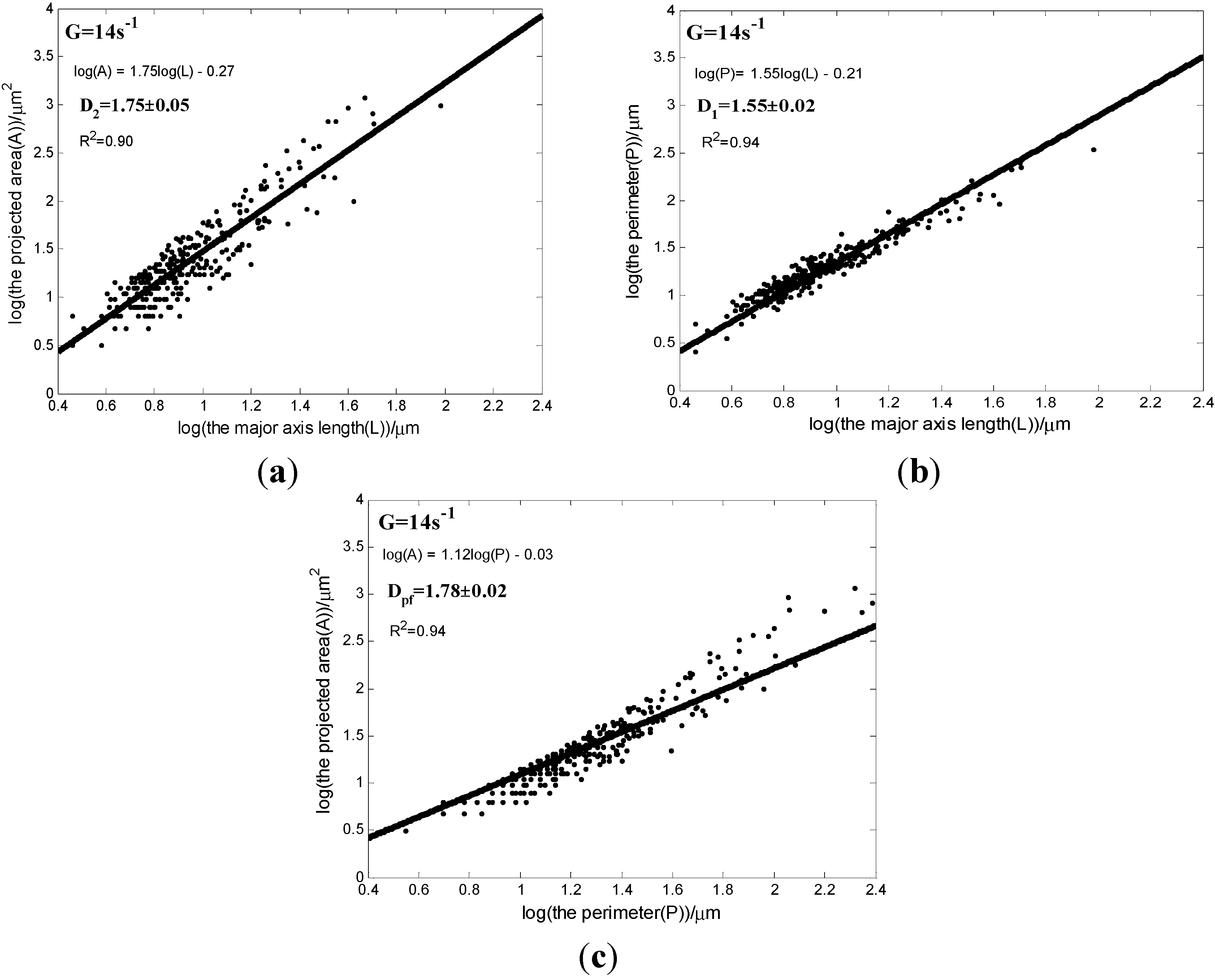
2.1. Fractal Dimension Analyses
2.2. Experiment Description
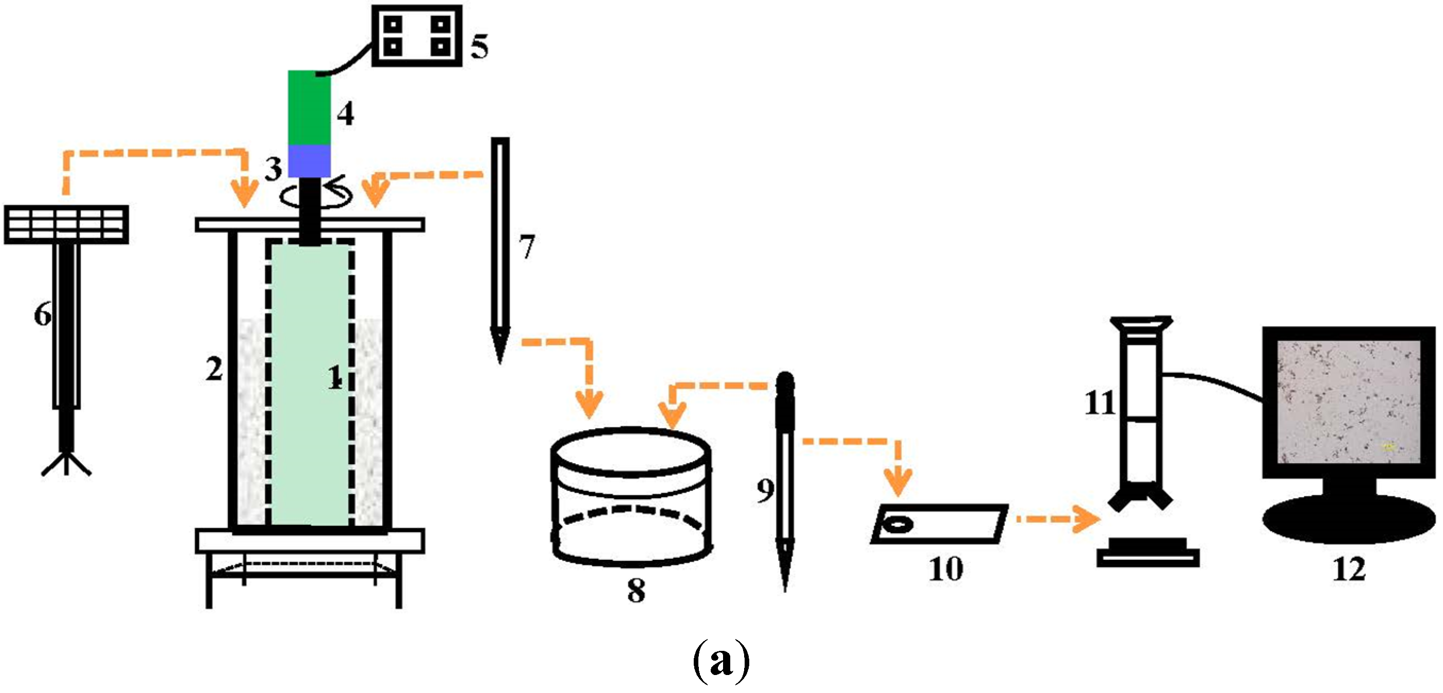
2.2.1. Turbulence-Generating Device
2.2.2. Shear Rate Calculation

| ω (rpm) | 24 | 27 | 42 | 60 | 90 | 120 | 150 | 180 |
|---|---|---|---|---|---|---|---|---|
| (mm/s) | 0 | 0 | 31.5 | 39.1 | 57.6 | 70.8 | 81.5 | 103.2 |
| G (s−1) | 5.36 | 5.96 | 9.17 | 14 | 24 | 31 | 41 | 53 |
| Pe | 406 | 452 | 695 | 1062 | 1820 | 2352 | 3110 | 4021 |
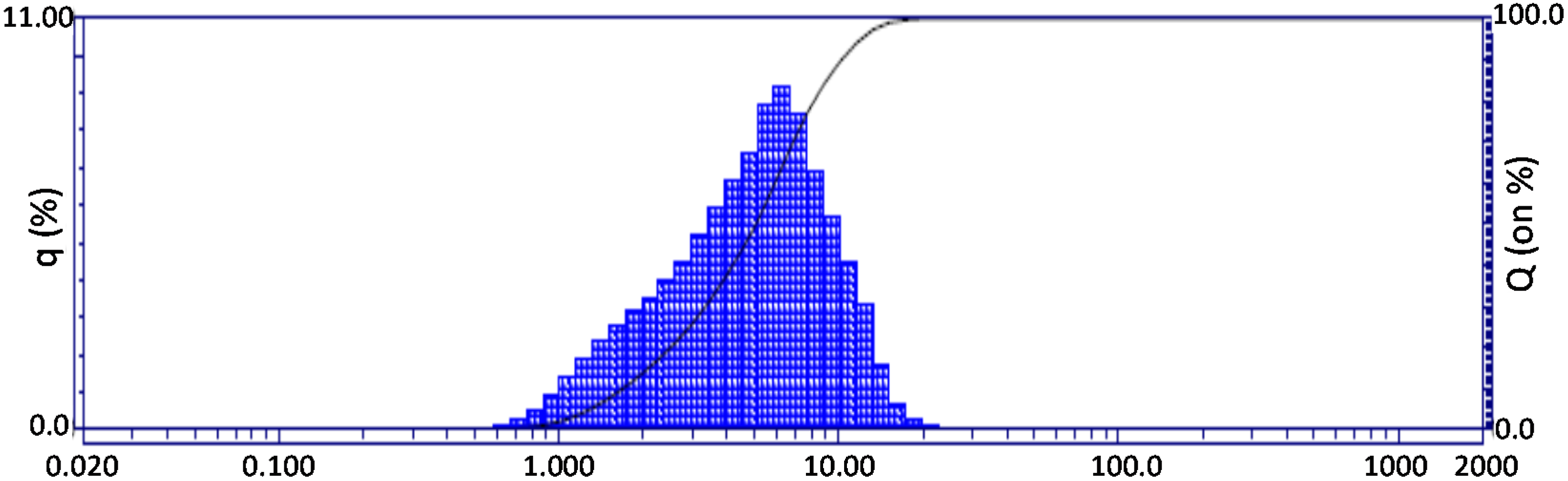
2.2.3. Sediment

| Sediment | Range (µm) | d10 (µm) | d30 (µm) | d50 (µm) | d70 (µm) | d90 (µm) |
|---|---|---|---|---|---|---|
| Primary particles | 0.59~23 | 1.7 | 3.36 | 5.07 | 6.89 | 10.27 |
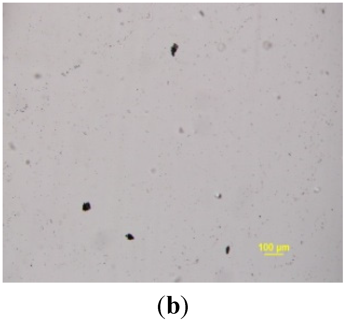
2.2.4. Experimental Procedure


3. Results and Discussions
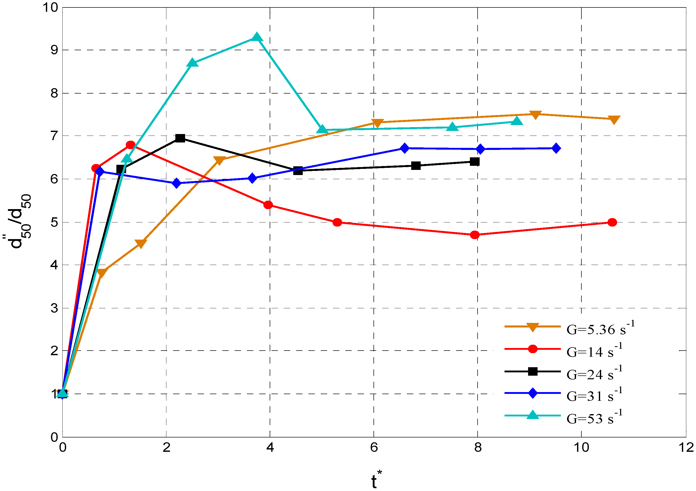
3.1. Attainment of Steady-State Flocculation Development
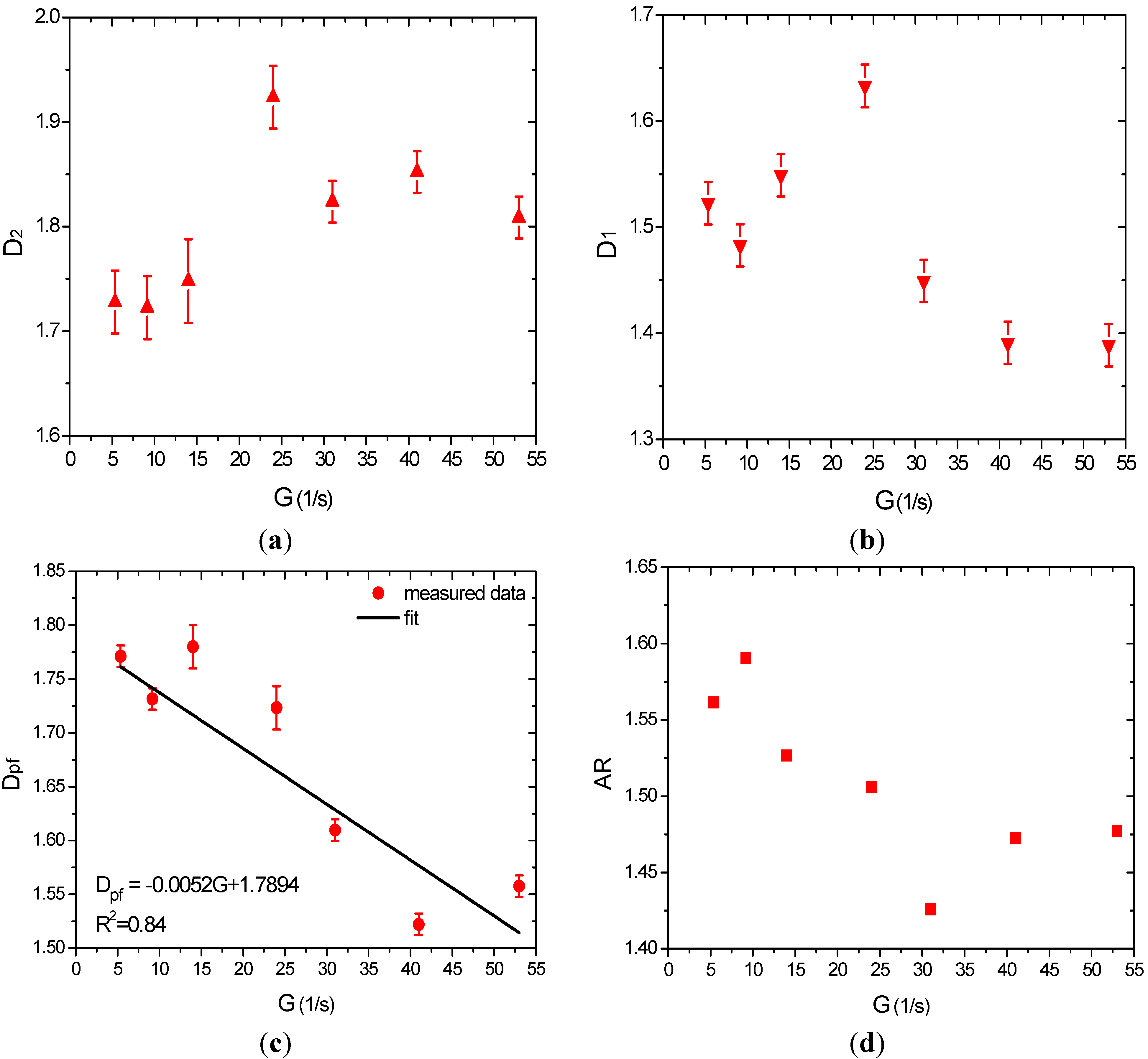
3.2. Fractal Dimension of the Flocs with Respect to Shear Rate

| G (s−1) | 5.36 | 9.17 | 14 | 24 | 31 | 41 | 53 |
|---|---|---|---|---|---|---|---|
| η (μm) | No | 330.23 | 267.26 | 204.12 | 179.61 | 156.17 | 137.36 |
| Maximum floc size (μm) | No | 51.11 | 134.71 | 101.05 | 73.45 | 64.67 | 55.13 |
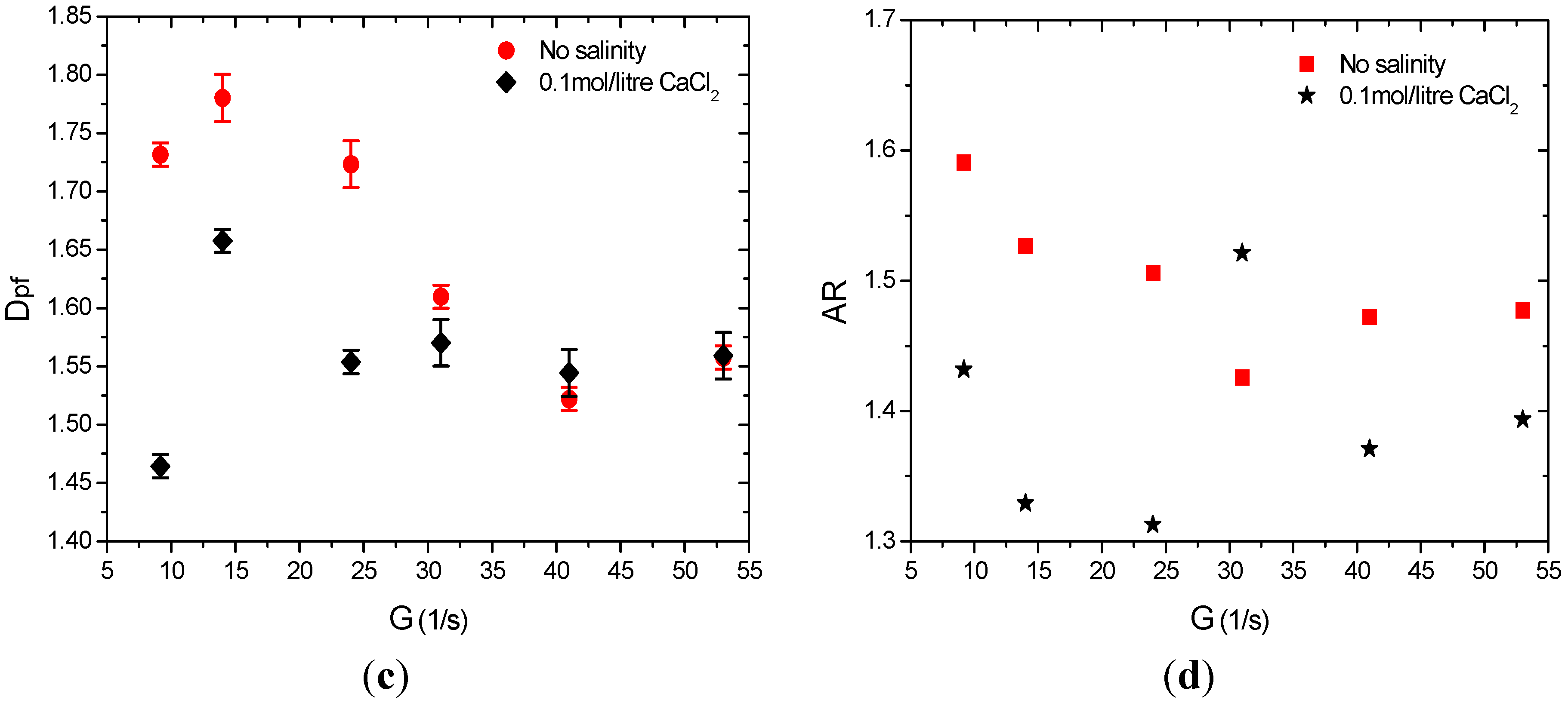
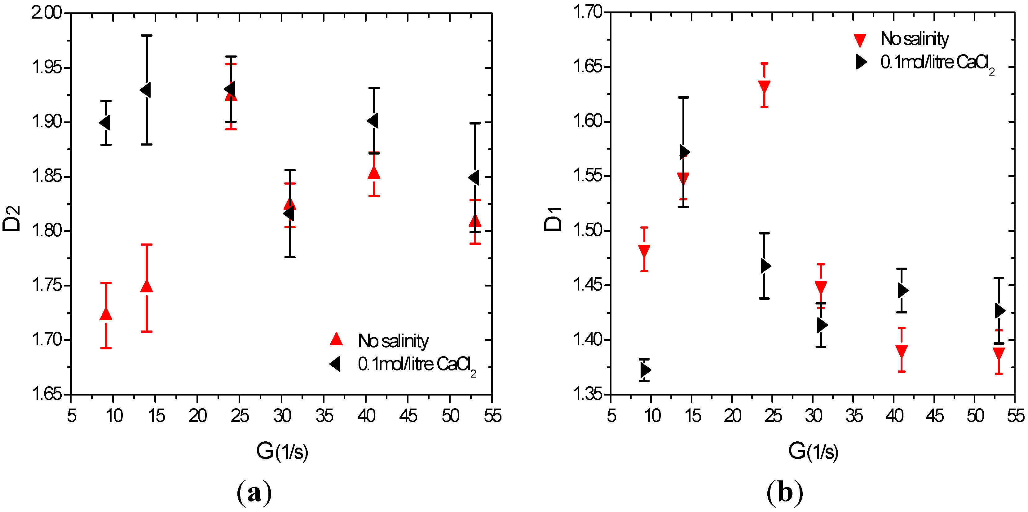
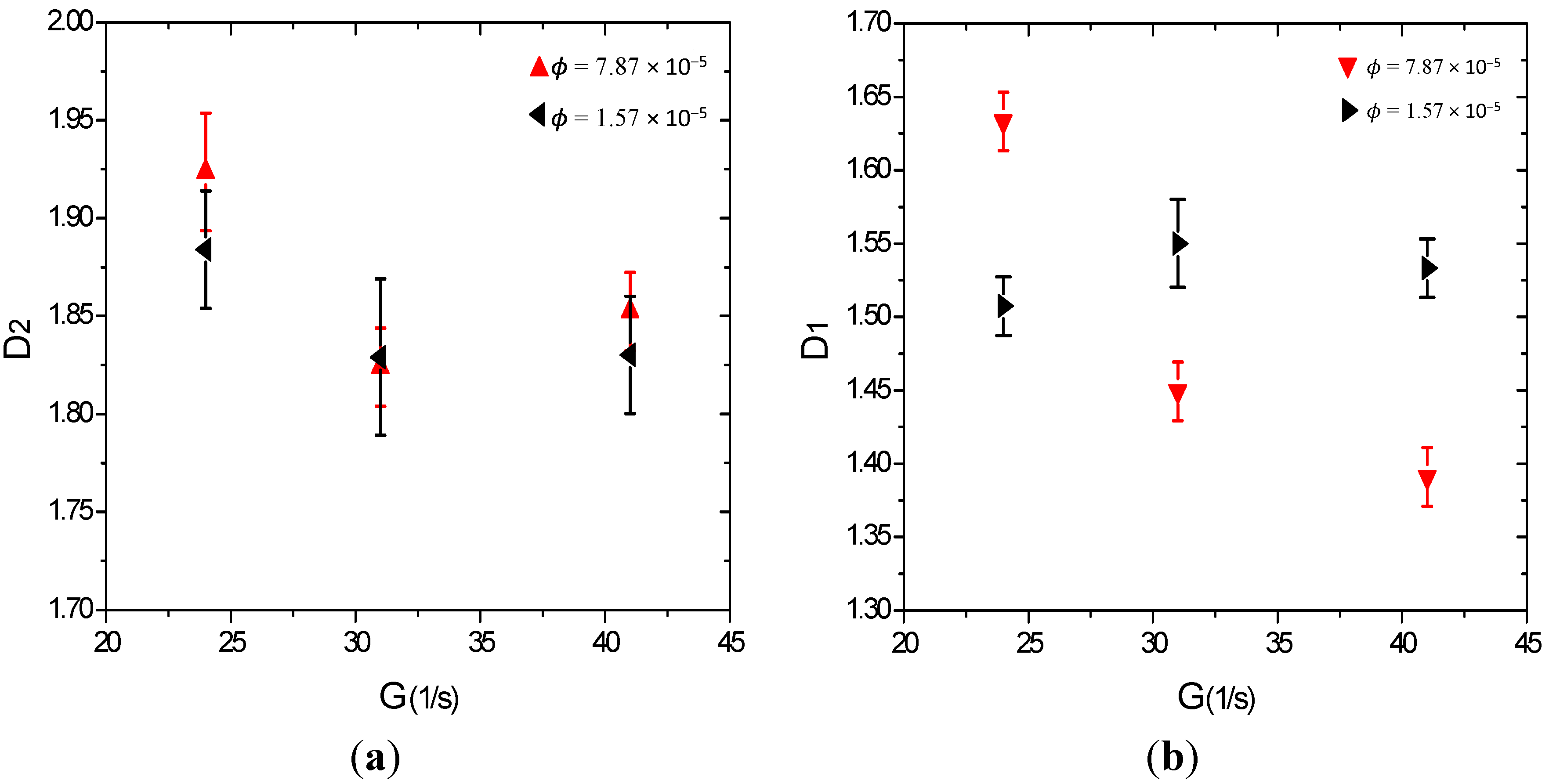
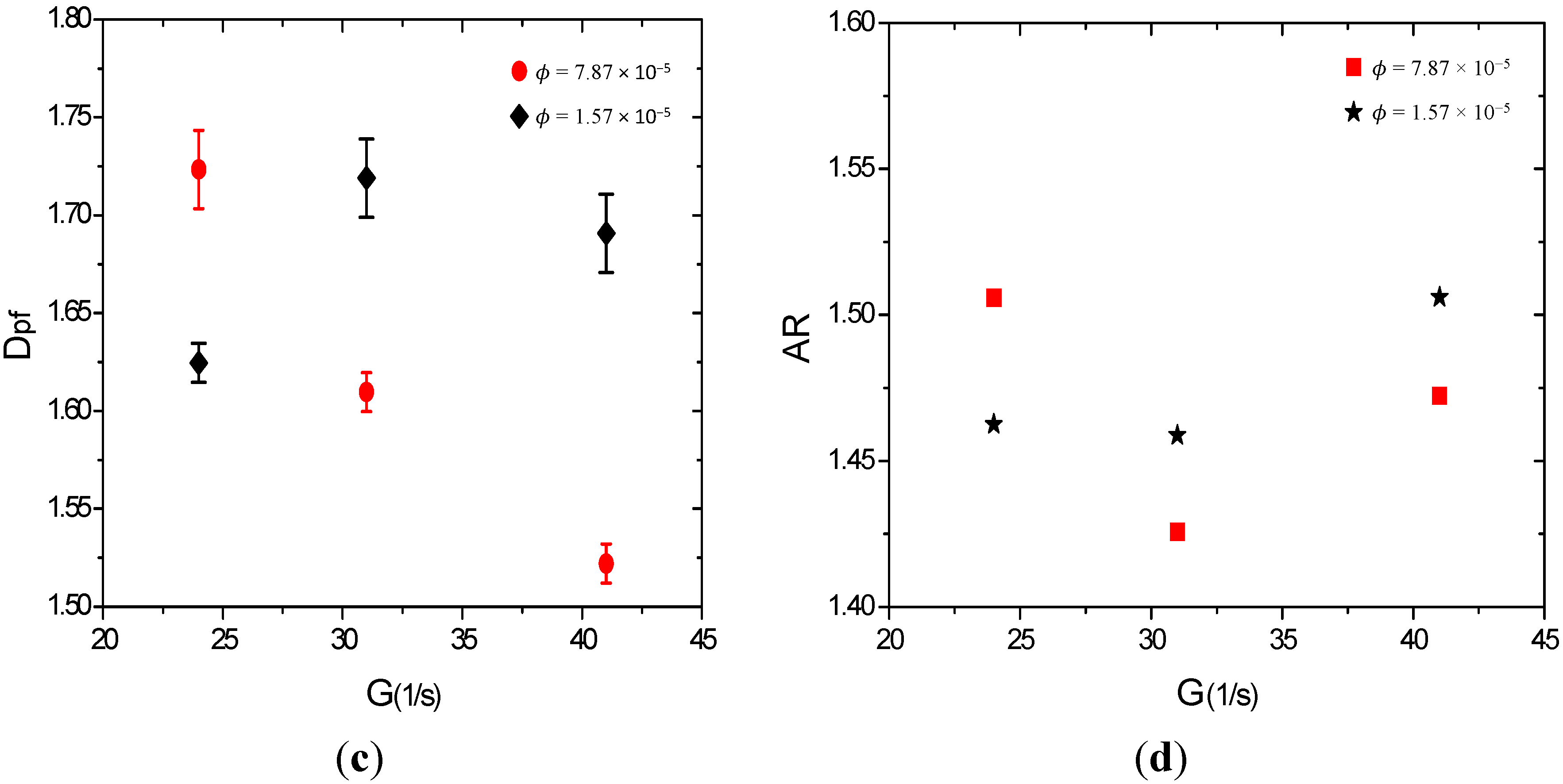
3.3. Effect of Electrolyte on Floc Fractal Dimension

3.4. Effect of Primary Sediment Concentration on Floc Fractal Dimension
4. Conclusions
- (1)
- With increasing shear stresses, the flocs become less elongated and less convoluted, and their boundary lines get tighter and more regular, caused by more breakages and possible restructurings of the flocs at high shear conditions.
- (2)
- As the electrolyte is added and initial sediment concentration goes up, the flocs become less elongated and more symmetrical, and their boundaries become less convoluted and simpler.
Acknowledgments
Author Contributions
Conflicts of Interest
References
- Winterwerp, J.C. A simple model for turbulence induced flocculation of cohesive sediment. J. Hydraul. Res. 1998, 36, 309–326. [Google Scholar] [CrossRef]
- Kranenburg, C. Effects of floc strength on viscosity and deposition of cohesive sediment suspensions. Cont. Shelf Res. 1999, 19, 1665–1680. [Google Scholar] [CrossRef]
- Thomas, D.; Judd, S.; Fawcett, N. Flocculation modelling: A review. Water Res. 1999, 33, 1579–1592. [Google Scholar] [CrossRef]
- Xu, F.; Wang, D.-P.; Riemer, N. Modeling flocculation processes of fine-grained particles using a size-resolved method: Comparison with published laboratory experiments. Cont. Shelf Res. 2008, 28, 2668–2677. [Google Scholar] [CrossRef]
- Dyer, K. Sediment processes in estuaries: Future research requirements. J. Geophys. Res. Oceans 1978–2012 1989, 94, 14327–14339. [Google Scholar]
- Mandelbrot, B.B. The Fractal Geometry of Nature; William H. Freeman: New York, NY, USA, 1983. [Google Scholar]
- Stone, M.; Krishnappan, B. Floc morphology and size distributions of cohesive sediment in steady-state flow. Water Res. 2003, 37, 2739–2747. [Google Scholar] [CrossRef]
- Serra, T.; Casamitjana, X. Structure of the aggregates during the process of aggregation and breakup under a shear flow. J.Colloid Interface Sci. 1998, 206, 505–511. [Google Scholar] [CrossRef] [PubMed]
- Bubakova, P.; Pivokonsky, M.; Filip, P. Effect of shear rate on aggregate size and structure in the process of aggregation and at steady state. Powder Technol. 2013, 235, 540–549. [Google Scholar] [CrossRef]
- Oles, V. Shear-induced aggregation and breakup of polystyrene latex particles. J. Colloid Interface Sci. 1992, 154, 351–358. [Google Scholar] [CrossRef]
- Spicer, P.T.; Keller, W.; Pratsinis, S.E. The effect of impeller type on floc size and structure during shear-induced flocculation. J. Colloid Interface Sci. 1996, 184, 112–122. [Google Scholar] [CrossRef] [PubMed]
- Serra, T.; Colomer, J.; Casamitjana, X. Aggregation and breakup of particles in a shear flow. J. Colloid Interface Sci. 1997, 187, 466–473. [Google Scholar] [CrossRef] [PubMed]
- Flesch, J.C.; Spicer, P.T.; Pratsinis, S.E. Laminar and turbulent shear—Induced flocculation of fractal aggregates. AIChE J. 1999, 45, 1114–1124. [Google Scholar] [CrossRef]
- Biggs, C.; Lant, P. Activated sludge flocculation: On-line determination of floc size and the effect of shear. Water Res. 2000, 34, 2542–2550. [Google Scholar] [CrossRef]
- Soos, M.; Wang, L.; Fox, R.; Sefcik, J.; Morbidelli, M. Population balance modeling of aggregation and breakage in turbulent taylor–couette flow. J. Colloid Interface Sci. 2007, 307, 433–446. [Google Scholar] [CrossRef] [PubMed]
- Ehrl, L.; Soos, M.; Morbidelli, M. Dependence of aggregate strength, structure, and light scattering properties on primary particle size under turbulent conditions in stirred tank. Langmuir 2008, 24, 3070–3081. [Google Scholar] [CrossRef] [PubMed]
- Ehrl, L.; Soos, M.; Morbidelli, M.; Bäbler, M.U. Dependence of initial cluster aggregation kinetics on shear rate for particles of different sizes under turbulence. AIChE J. 2009, 55, 3076–3087. [Google Scholar] [CrossRef]
- Ehrl, L.; Soos, M.; Wu, H.; Morbidelli, M. Effect of flow field heterogeneity in coagulators on aggregate size and structure. AIChE J. 2010, 56, 2573–2587. [Google Scholar] [CrossRef]
- Keyvani, A.; Strom, K. Influence of cycles of high and low turbulent shear on the growth rate and equilibrium size of mud flocs. Mar. Geol. 2014, 354, 1–14. [Google Scholar] [CrossRef]
- Selomulya, C.; Bushell, G.; Amal, R.; Waite, T. Understanding the role of restructuring in flocculation: The application of a population balance model. Chem. Eng. Sci. 2003, 58, 327–338. [Google Scholar] [CrossRef]
- Williams, R.; Peng, S.; Naylor, A. In situ measurement of particle aggregation and breakage kinetics in a concentrated suspension. Powder Technol. 1992, 73, 75–83. [Google Scholar] [CrossRef]
- Selomulya, C.; Amal, R.; Bushell, G.; Waite, T.D. Evidence of shear rate dependence on restructuring and breakup of latex aggregates. J. Colloid Interface Sci. 2001, 236, 67–77. [Google Scholar] [CrossRef] [PubMed]
- Hopkins, D.C.; Ducoste, J.J. Characterizing flocculation under heterogeneous turbulence. J. Colloid Interface Sci. 2003, 264, 184–194. [Google Scholar] [CrossRef]
- Rahmani, N.H.; Masliyah, J.H.; Dabros, T. Characterization of asphaltenes aggregation and fragmentation in a shear field. AIChE J. 2003, 49, 1645–1655. [Google Scholar] [CrossRef]
- Logan, B.E.; Kilps, J.R. Fractal dimensions of aggregates formed in different fluid mechanical environments. Water Res. 1995, 29, 443–453. [Google Scholar] [CrossRef]
- Jiang, Q.; Logan, B.E. Fractal dimensions of aggregates determined from steady-state size distributions. Environ. Sci. Technol. 1991, 25, 2031–2038. [Google Scholar] [CrossRef]
- Spicer, P.T.; Pratsinis, S.E. Shear-induced flocculation: The evolution of floc structure and the shape of the size distribution at steady state. Water Res. 1996, 30, 1049–1056. [Google Scholar] [CrossRef]
- Mandelbrot, B.B.; Passoja, D.E.; Paullay, A.J. Fractal character of fracture surfaces of metals. Nature 1984, 308, 721–722. [Google Scholar] [CrossRef]
- Serra, T.; Colomer, J.; Logan, B.E. Efficiency of different shear devices on flocculation. Water Res. 2008, 42, 1113–1121. [Google Scholar] [CrossRef] [PubMed]
- Bouyer, D.; Line, A.; Cockx, A.; Do-Quang, Z. Experimental analysis of floc size distribution and hydrodynamics in a jar-test. Chem. Eng. Res. Des. 2001, 79, 1017–1024. [Google Scholar] [CrossRef]
- Colomer, J.; Peters, F.; Marrasé, C. Experimental analysis of coagulation of particles under low-shear flow. Water Res. 2005, 39, 2994–3000. [Google Scholar] [CrossRef] [PubMed]
- Winterwerp, J. On the flocculation and settling velocity of estuarine mud. Cont. Shelf Res. 2002, 22, 1339–1360. [Google Scholar] [CrossRef]
- Camp, T.R.; Stein, P.C. Velocity gradients and internal work in fluid motion. J. Boston Soc.Civil Eng. 1943, 85, 219–237. [Google Scholar]
- Hinze, J.O. Turbulence, 2nd ed.; McGraw-Hill: New York, NY, USA, 1975. [Google Scholar]
- Zhu, Z. The Investigation on Phase Transition and the Influence of Shear on the Flocculation of Cohesive Sediment. Master’s Thesis, Tsinghua University, Beijing, China, 2009. [Google Scholar]
- Lazier, J.; Mann, K. Turbulence and the diffusive layers around small organisms. Deep Sea Res. Part A. Oceanogr. Res. Pap. 1989, 36, 1721–1733. [Google Scholar] [CrossRef]
- Bowen, J.D.; Stolzenbach, K.D.; Chisholm, S.W. Simulating bacterial clustering around phytoplankton cells in a turbulent ocean. Limnol. Oceanogr. 1993, 38, 36–51. [Google Scholar] [CrossRef]
- Kumar, R.G.; Strom, K.B.; Keyvani, A. Floc properties and settling velocity of san jacinto estuary mud under variable shear and salinity conditions. Cont. Shelf Res. 2010, 30, 2067–2081. [Google Scholar] [CrossRef]
- Kiørboe, T.; Saiz, E. Planktivorous feeding in calm and turbulent environments, with emphasis on copepods. Mar. Ecol. Prog. Ser. 1995, 122, 135–145. [Google Scholar] [CrossRef]
- Lick, W.; Lick, J. Aggregation and disaggregation of fine-grained lake sediments. J. Great Lakes Res. 1988, 14, 514–523. [Google Scholar] [CrossRef]
- Burban, P.Y.; Lick, W.; Lick, J. The flocculation of fine—Grained sediments in estuarine waters. J. Geophys. Res. Ocean. 1978–2012 1989, 94, 8323–8330. [Google Scholar] [CrossRef]
- Estrada, M.; Berdalet, E. Phytoplankton in a turbulent world. Sci. Mar. 1997, 61, 125–140. [Google Scholar]
- Crittenden, J.C.; Trussell, R.R.; Hand, D.W.; Howe, K.J.; Tchobanoglous, G. Mwh’s Water Treatment: Principles and Design, 2nd ed.; John Wiley & Sons: Hoboken, NJ, USA, 2005. [Google Scholar]
- Chandrasekhar, S. Hydrodynamic and Hydromagnetic Stability; Clarendon Press: Oxford, UK, 1961; Volume 196. [Google Scholar]
- Maggi, F. Variable fractal dimension: A major control for floc structure and flocculation kinematics of suspended cohesive sediment. J. Geophys. Res. Ocean. 1978–2012 2007, 112. [Google Scholar] [CrossRef]
- Maggi, F.; Mietta, F.; Winterwerp, J. Effect of variable fractal dimension on the floc size distribution of suspended cohesive sediment. J. Hydrol. 2007, 343, 43–55. [Google Scholar] [CrossRef]
- Tambo, N.; Watanabe, Y. Physical aspect of flocculation process—I: Fundamental treatise. Water Res. 1979, 13, 429–439. [Google Scholar] [CrossRef]
- Francois, R. Growth kinetics of hydroxide flocs. J. Am. Water Works Assoc. 1988, 80, 92–96. [Google Scholar]
- Gibbs, R.J.; Konwar, L.N. Effect of pipetting on mineral flocs. Environ. Sci. Technol. 1982, 16, 119–121. [Google Scholar] [CrossRef]
- Lick, W.; Huang, H.; Jepsen, R. Flocculation of fine—Grained sediments due to differential settling. J. Geophys. Res. Ocean. 1978–2012 1993, 98, 10279–10288. [Google Scholar] [CrossRef]
- Stolzenbach, K.D.; Elimelech, M. The effect of particle density on collisions between sinking particles: Implications for particle aggregation in the ocean. Deep Sea Res. Part I Oceanogr. Res. Pap. 1994, 41, 469–483. [Google Scholar] [CrossRef]
- Son, M.; Hsu, T.-J. Flocculation model of cohesive sediment using variable fractal dimension. Environ. Fluid Mech. 2008, 8, 55–71. [Google Scholar] [CrossRef]
- Son, M.; Hsu, T.-J. The effect of variable yield strength and variable fractal dimension on flocculation of cohesive sediment. Water Res. 2009, 43, 3582–3592. [Google Scholar] [CrossRef] [PubMed]
- Smoluchowski, M. Mathematical theory of the kinetics of the coagulation of colloidal solutions. Z. Phys. Chem. 1917, 92, 129. [Google Scholar]
- Prat, O.P.; Ducoste, J.J. Modeling spatial distribution of floc size in turbulent processes using the quadrature method of moment and computational fluid dynamics. Chem. Eng. Sci. 2006, 61, 75–86. [Google Scholar] [CrossRef]
- Kusters, K.A.; Wijers, J.G.; Thoenes, D. Aggregation kinetics of small particles in agitated vessels. Chem. Eng. Sci. 1997, 52, 107–121. [Google Scholar] [CrossRef]
- Francois, R. Strength of aluminium hydroxide flocs. Water Res. 1987, 21, 1023–1030. [Google Scholar] [CrossRef]
- Winterwerp, J.; Manning, A.; Martens, C.; de Mulder, T.; Vanlede, J. A heuristic formula for turbulence-induced flocculation of cohesive sediment. Estuar. Coast. Shelf Sci. 2006, 68, 195–207. [Google Scholar] [CrossRef]
- Gorczyca, B.; Ganczarczyk, J. Image analysis of alum coagulated mineral suspensions. Environ. Technol. 1996, 17, 1361–1369. [Google Scholar] [CrossRef]
- De Boer, D.H. An evaluation of fractal dimensions to quantify changes in the morphology of fluvial suspended sediment particles during baseflow conditions. Hydrol. Process. 1997, 11, 415–426. [Google Scholar]
- Li, D.H.; Ganczarczyk, J. Fractal geometry of particle aggregates generated in water and wastewater treatment processes. Environ. Sci. Technol. 1989, 23, 1385–1389. [Google Scholar] [CrossRef]
- De Boer, D.H.; Stone, M. Fractal dimensions of suspended solids in streams: Comparison of sampling and analysis techniques. Hydrol. Process. 1999, 13, 239–254. [Google Scholar]
- Manning, A.; Dyer, K. A laboratory examination of floc characteristics with regard to turbulent shearing. Mar. Geol. 1999, 160, 147–170. [Google Scholar] [CrossRef]
- Tang, S.; Ma, Y.; Shiu, C. Modelling the mechanical strength of fractal aggregates. Colloids Surf. A Physicochem. Eng. Asp. 2001, 180, 7–16. [Google Scholar] [CrossRef]
© 2015 by the authors; licensee MDPI, Basel, Switzerland. This article is an open access article distributed under the terms and conditions of the Creative Commons Attribution license (http://creativecommons.org/licenses/by/4.0/).
Share and Cite
Zhu, Z.; Yu, J.; Wang, H.; Dou, J.; Wang, C. Fractal Dimension of Cohesive Sediment Flocs at Steady State under Seven Shear Flow Conditions. Water 2015, 7, 4385-4408. https://doi.org/10.3390/w7084385
Zhu Z, Yu J, Wang H, Dou J, Wang C. Fractal Dimension of Cohesive Sediment Flocs at Steady State under Seven Shear Flow Conditions. Water. 2015; 7(8):4385-4408. https://doi.org/10.3390/w7084385
Chicago/Turabian StyleZhu, Zhongfan, Jingshan Yu, Hongrui Wang, Jie Dou, and Cheng Wang. 2015. "Fractal Dimension of Cohesive Sediment Flocs at Steady State under Seven Shear Flow Conditions" Water 7, no. 8: 4385-4408. https://doi.org/10.3390/w7084385