Defining an Ecologically Ideal Shallow Groundwater Depth for Regional Sustainable Management: Conceptual Development and Case Study on the Sanjiang Plain, Northeast China


Abstract
:1. Introduction
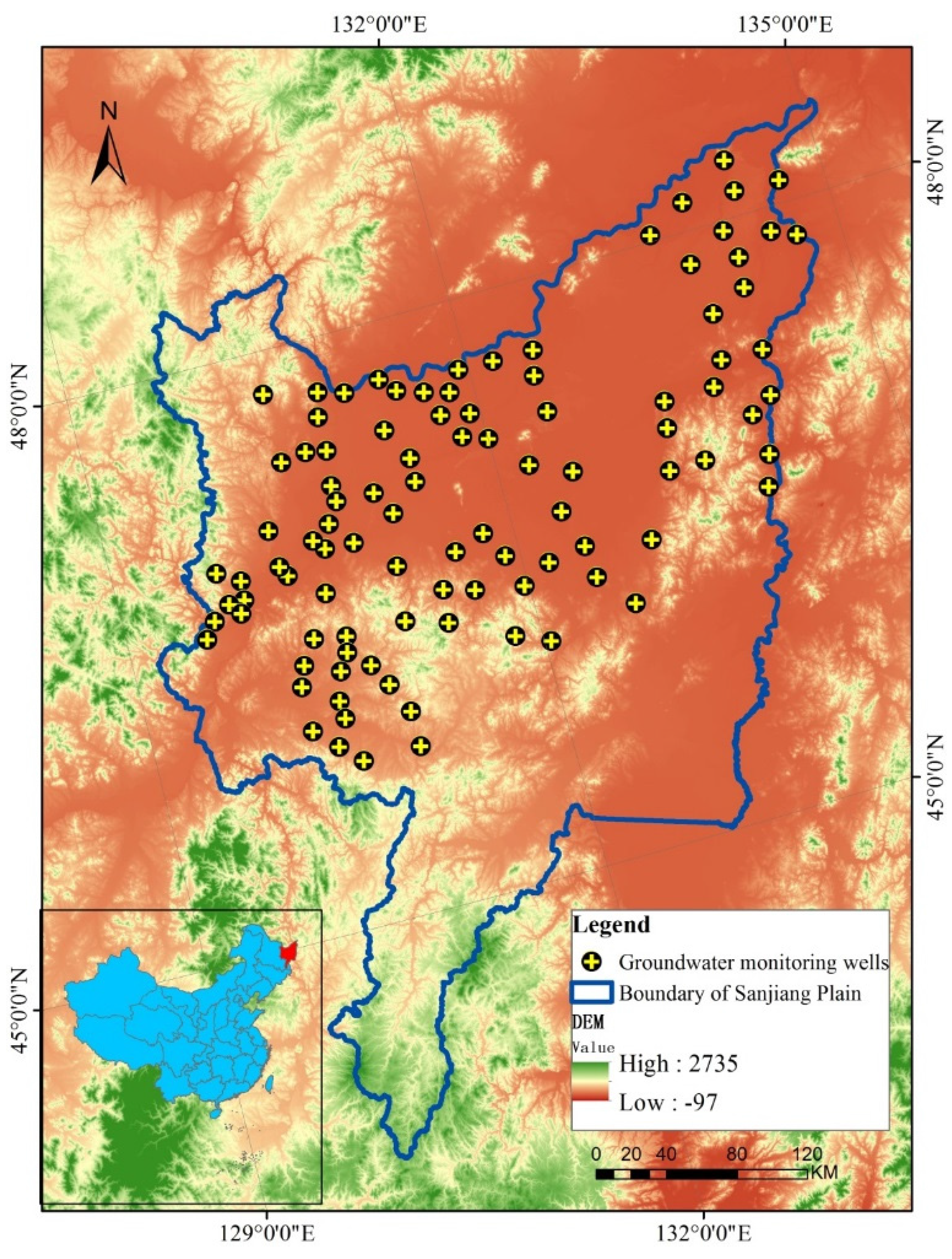
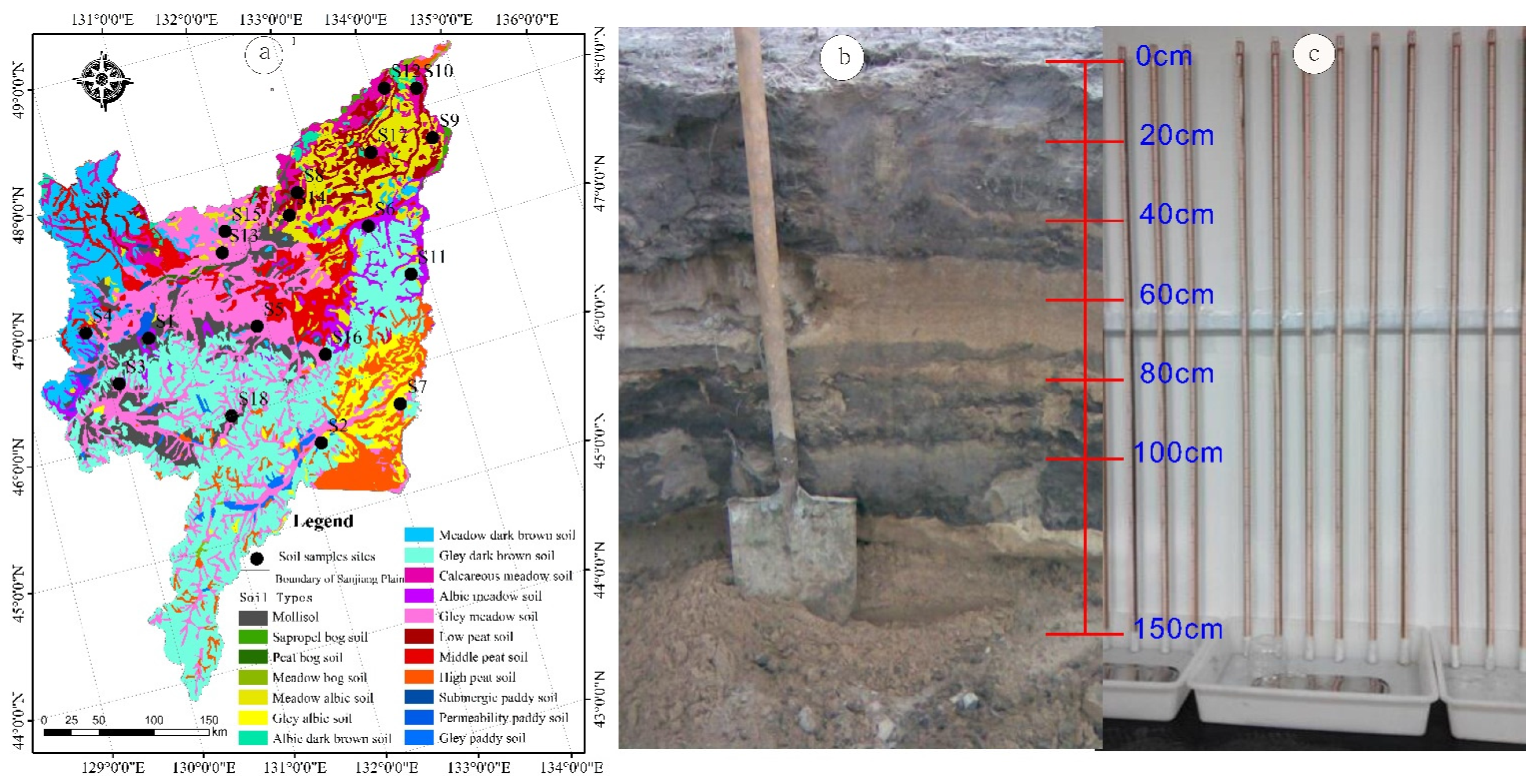
2. Study Area
3. Methodology
3.1. Conceptual Framework of an Ecologically Ideal Shallow Groundwater Depth (EISDG)

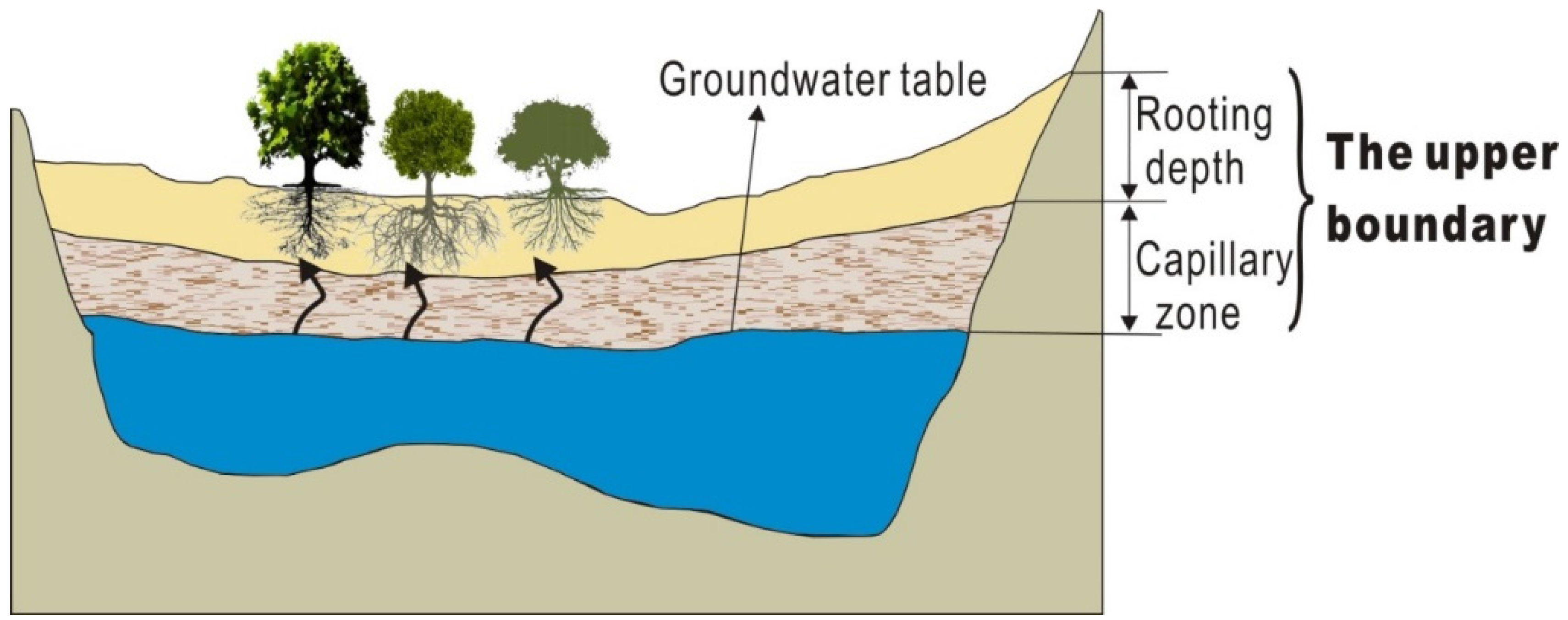
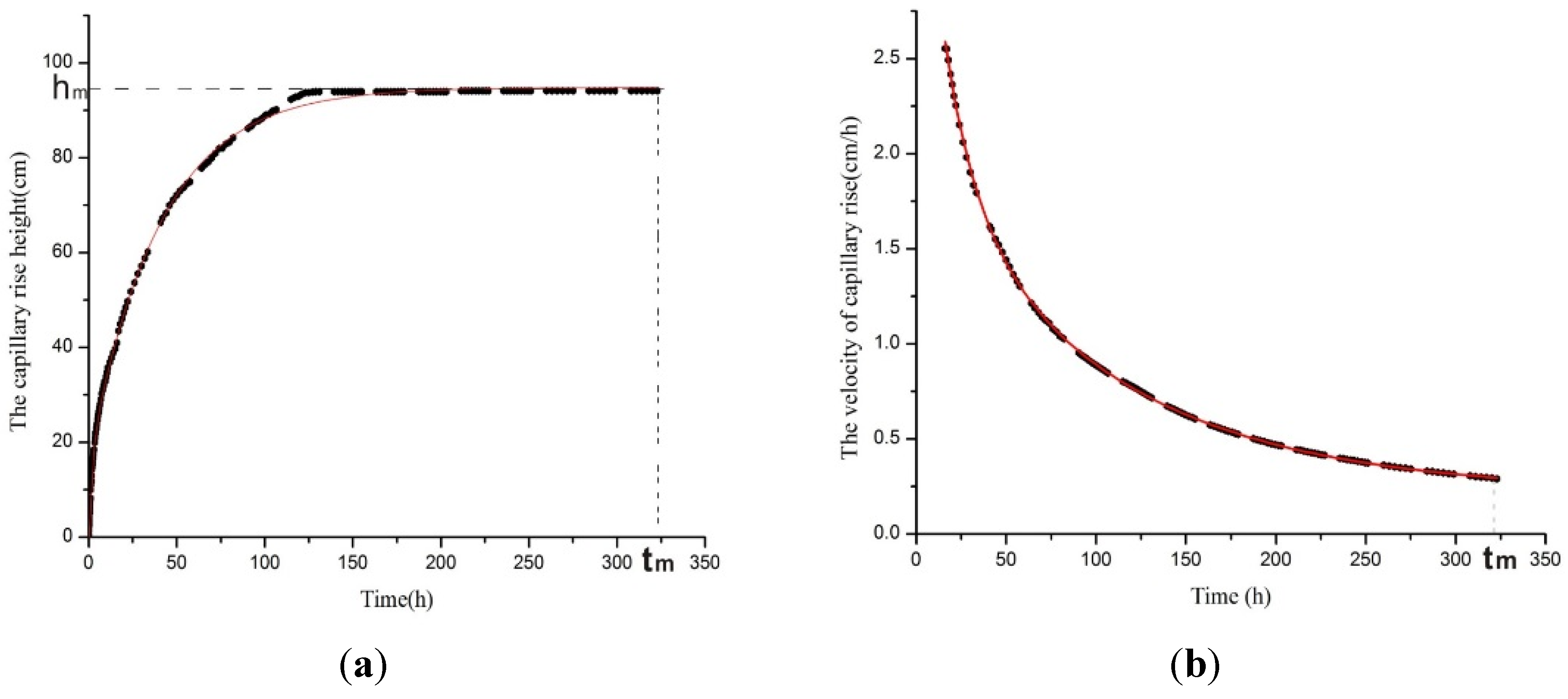
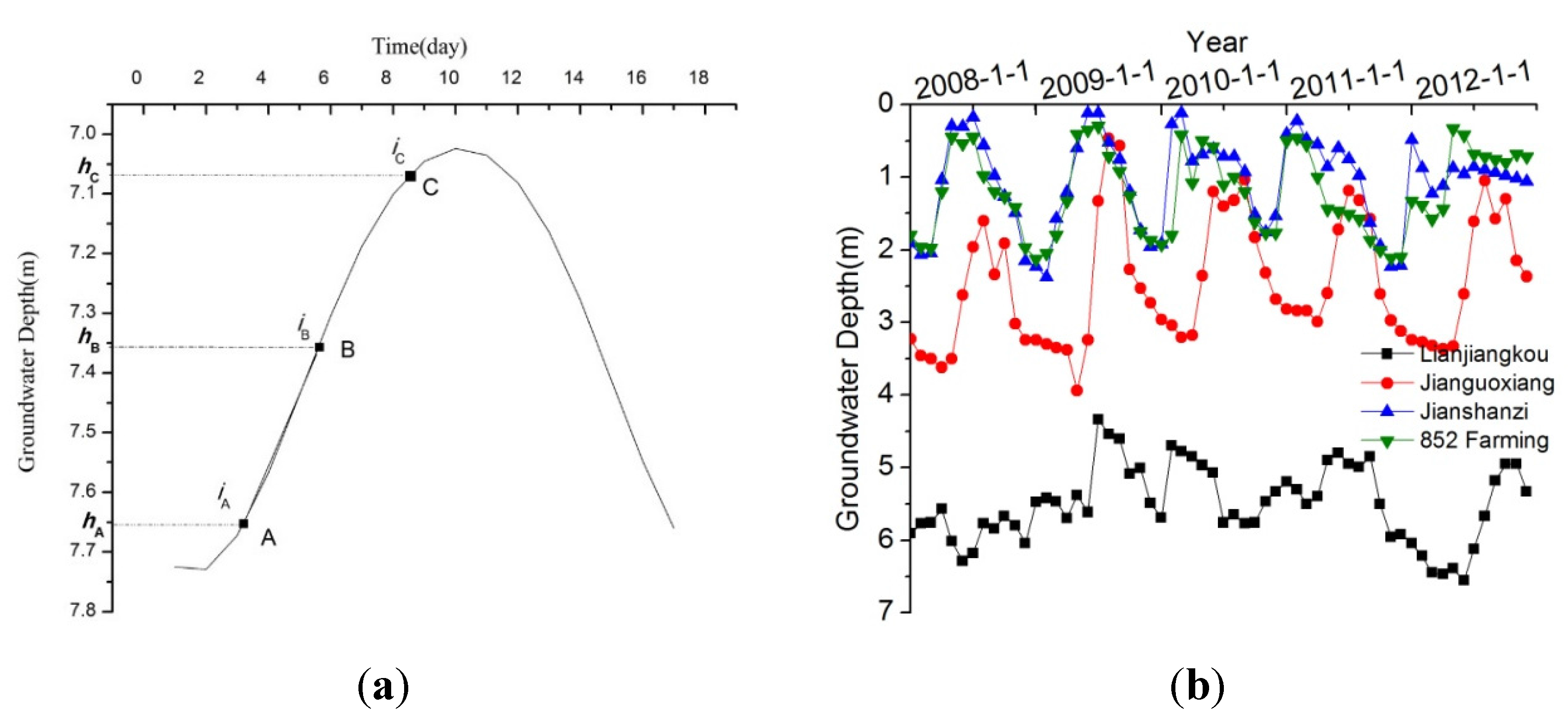
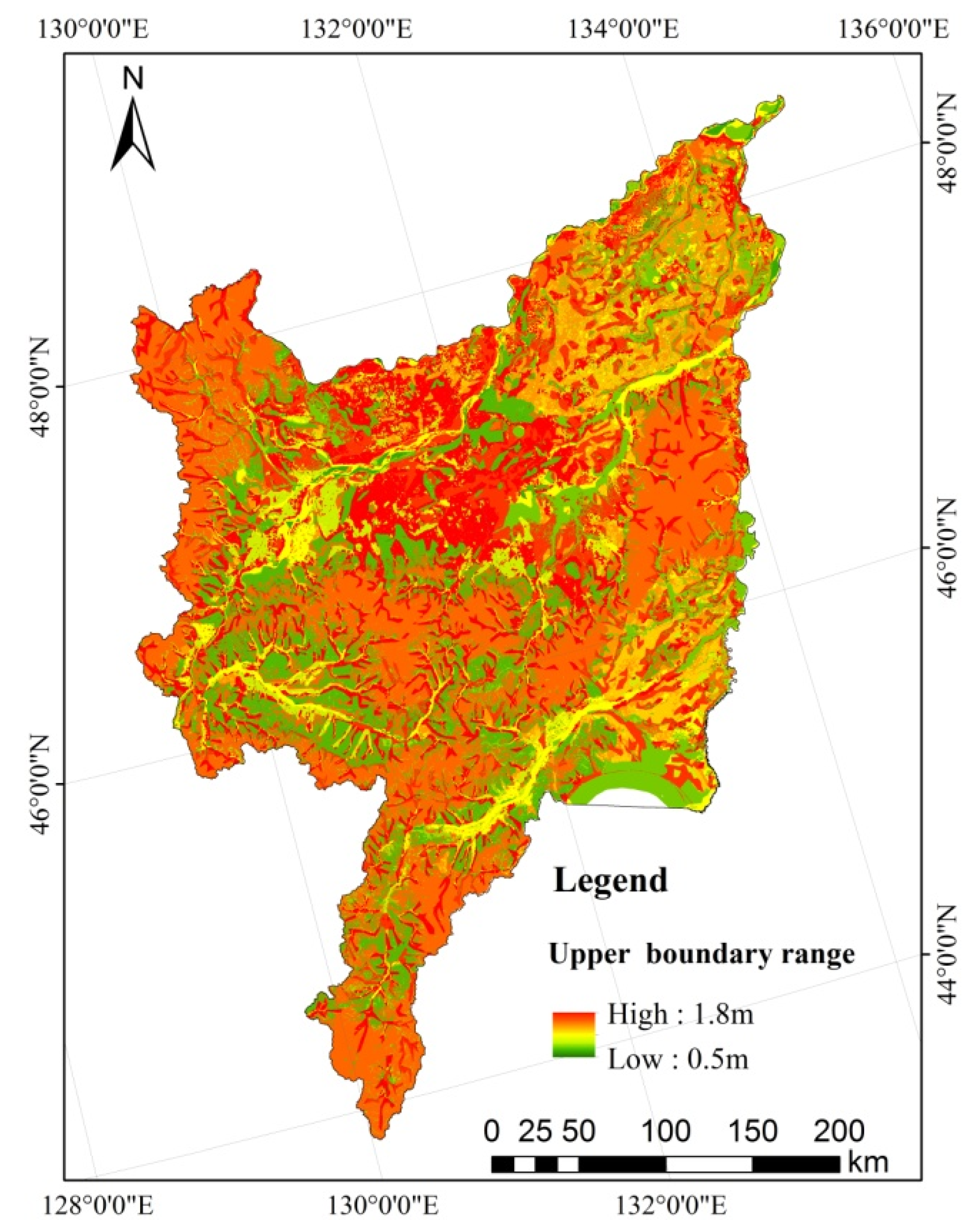
3.1.1. Determining the Upper Boundary of EISGD
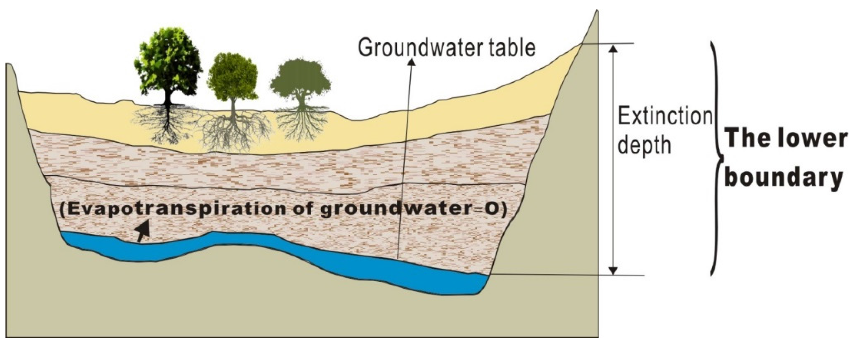
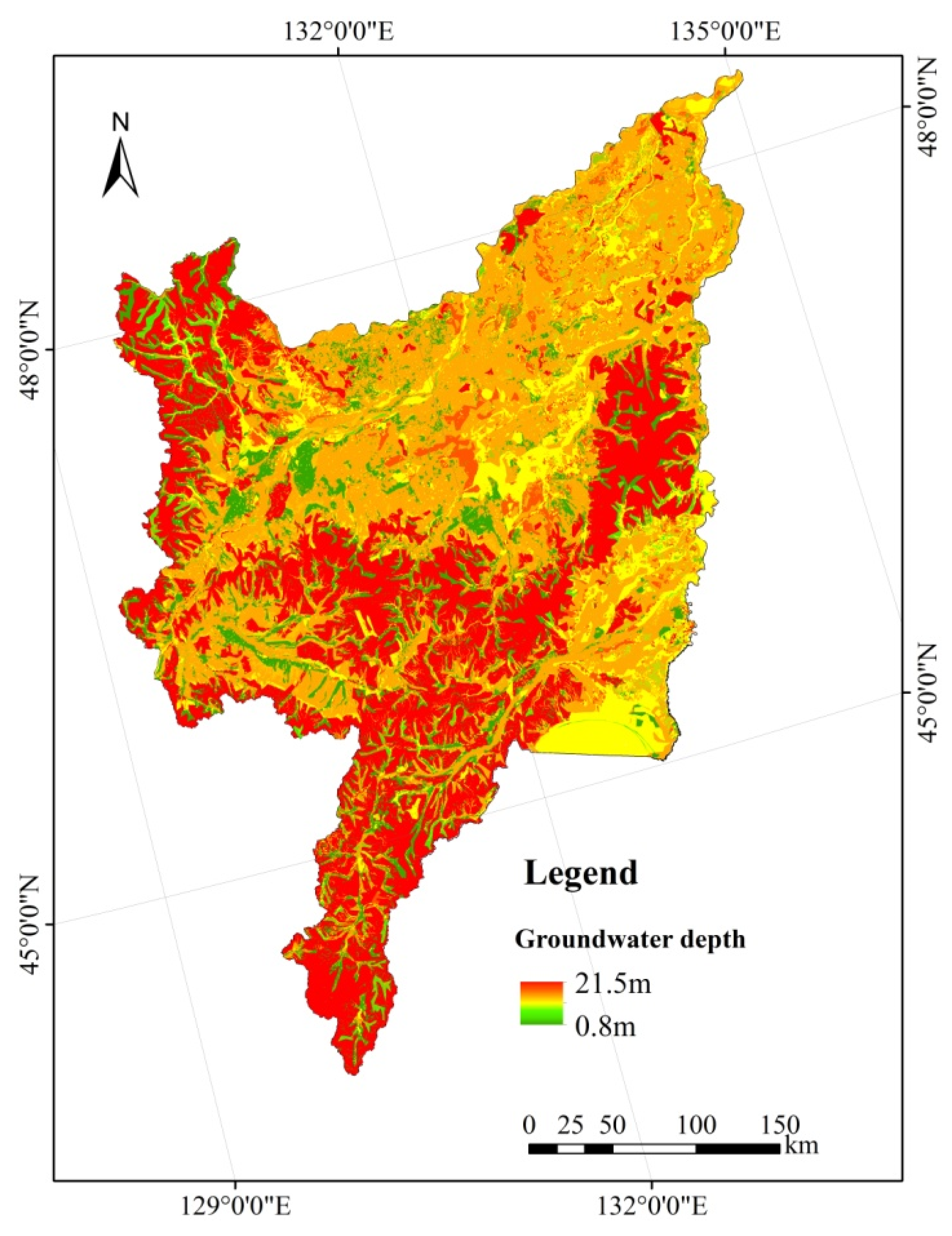
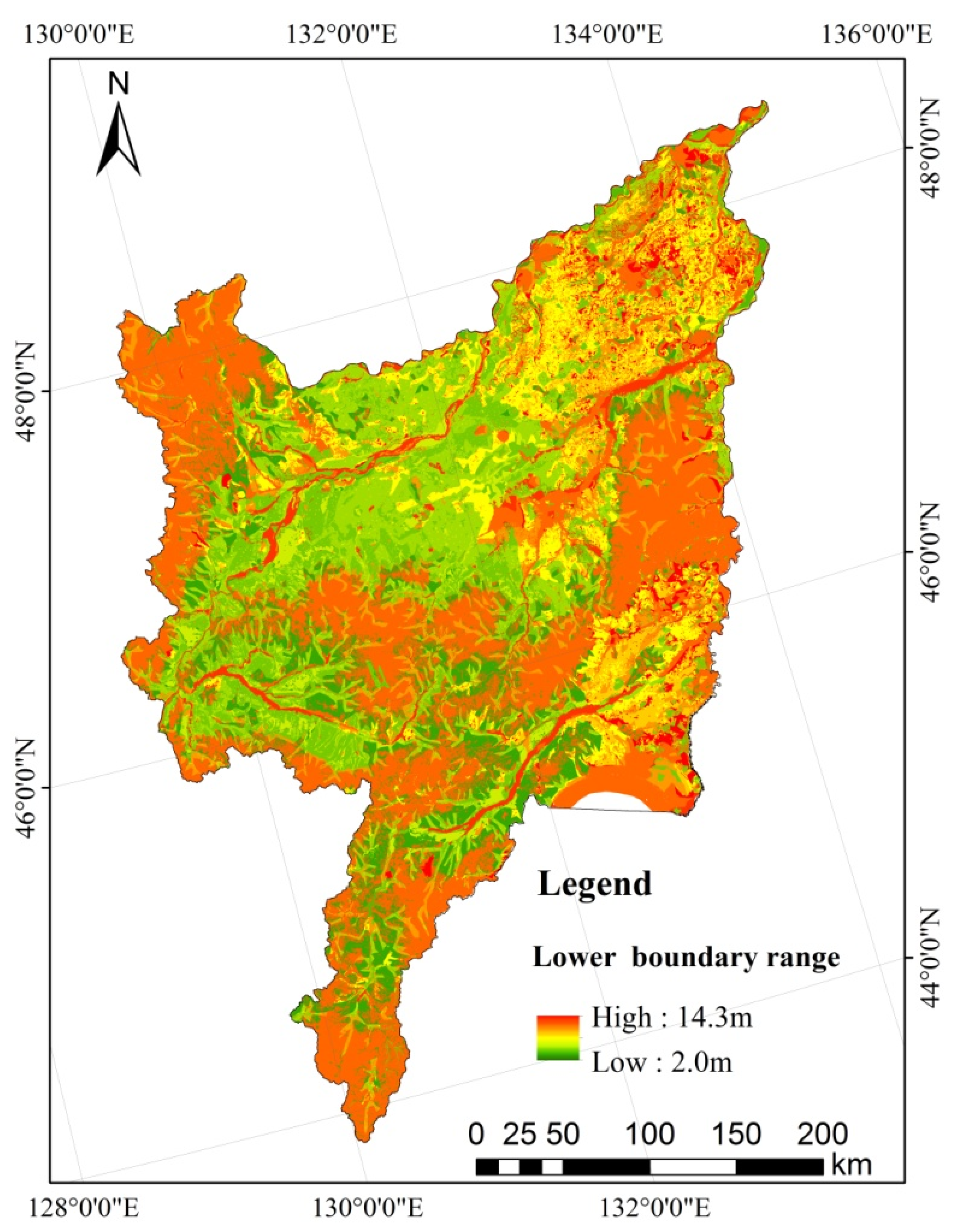
3.1.2. Determining the Lower Boundary of EISGD


3.3. Data Collection
3.4. Field Survey and Sampling


| Main Plants | Rooting Depth/m |
|---|---|
| Rice | 0.2 |
| Corn | 0.4 |
| Bean | 0.2 |
| Negundo artemisia | 0.1 |
| Green bristlegrass | 0.3 |
| Lespedeza | 1.8 |
| Moraceae | 2.2 |
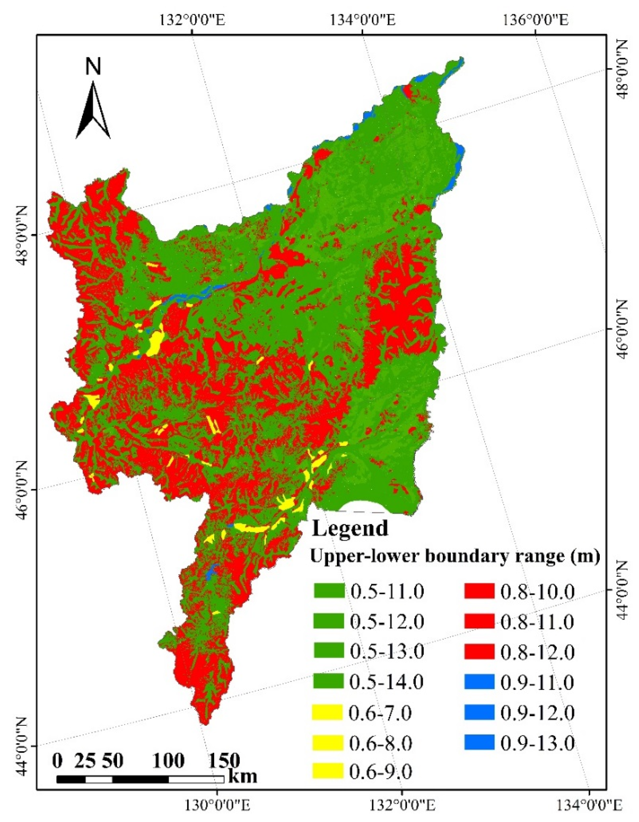
3.5. EISGD Boundary Mapping and Regional Assessment

3.6. Allowable Withdrawal of EISGD-Based Shallow Groundwater
4. Results
4.1. Boundary of EISGD
| City | Well ID | Lower of EISGD/m | Mean/m |
|---|---|---|---|
| Fuyuan | 10178180.00 | 10.5 | 12.1 |
| 10178080.00 | 6.2 | ||
| 10500400.00 | 9.5 | ||
| 10178060.00 | 10.6 | ||
| 10178090.00 | 18.5 | ||
| 10178110.00 | 22.4 | ||
| 10178140.00 | 10.6 | ||
| 10178100.00 | 8.1 | ||
| 10178170.00 | 12.5 | ||
| Raohe | 10561040.00 | 9.8 | 8.7 |
| 10561040.00 | 8.4 | ||
| 10561110.00 | 7.6 | ||
| 10561070.00 | 7.4 | ||
| 10500330.00 | 8.3 | ||
| 110561080.00 | 8.6 | ||
| 10500020.00 | 8.2 | ||
| 10561190.00 | 9.3 | ||
| 10561220.00 | 9.6 | ||
| 10561230.00 | 9.7 | ||
| Baoqing | 10573040.00 | 2.9 | 2.3 |
| 10573140.00 | 1.7 | ||
| 10573080.00 | 1.9 | ||
| 10573060.00 | 1.9 | ||
| 10573010.00 | 1.8 | ||
| 10573050.00 | 2.0 | ||
| 10573120.00 | 2.6 | ||
| 10573110.00 | 2.3 | ||
| 10573070.00 | 2.8 | ||
| 10573200.00 | 2.9 | ||
| Fujin | 10577150.00 | 6.9 | 7.3 |
| 10577110.00 | 7.5 | ||
| 10577190.00 | 7.6 | ||
| 10700151.00 | 7.2 | ||
| Youyi | 10575060.00 | 6.1 | 7.8 |
| 10575030.00 | 9.5 | ||
| Shuangyashan | 11168020.00 | 4.8 | 3.5 |
| 11168040.00 | 3.6 | ||
| 11168030.00 | 2.2 | ||
| Jixian | 11100592.00 | 18.9 | 14.8 |
| 11169010.00 | 10.7 | ||
| Huachuan | 10779050.00 | 9.3 | 7.1 |
| 10779030.00 | 4.9 | ||
| 10779020.00 | 8.6 | ||
| 10779070.00 | 5.2 | ||
| 10779060.00 | 6.5 | ||
| 10779040.00 | 7.8 | ||
| Suibin | 10779531.00 | 7.0 | 8.2 |
| 10100140.00 | 9.1 | ||
| 10779550.00 | 7.0 | ||
| 10779570.00 | 7.7 | ||
| 10779580.00 | 8.5 | ||
| 10779540.00 | 8.4 | ||
| 10779520.00 | 9.0 | ||
| 10779650.00 | 9.1 | ||
| Luobei | 10471050.00 | 9.1 | 8.1 |
| 10471120.00 | 6.6 | ||
| 10471030.00 | 7.2 | ||
| 10471020.00 | 7.6 | ||
| 10471130.00 | 7.4 | ||
| 10471100.00 | 8.6 | ||
| 10471080.00 | 9.2 | ||
| 11100540.00 | 8.7 | ||
| Jiamusi | 10778430.00 | 7.8 | 8.6 |
| 10700120.00 | 9.3 | ||
| 10778470.00 | 8.2 | ||
| 10778040.00 | 8.6 | ||
| 10778030.00 | 9.2 | ||
| Tangyuan | 11165030.00 | 8.5 | 7.7 |
| 11100520.00 | 6.6 | ||
| 11100520.00 | 7.2 | ||
| 11165060.00 | 7.6 | ||
| 11165090.00 | 8.5 | ||
| 11165120.00 | 6.9 | ||
| 11165080.00 | 7.8 | ||
| 11165160.00 | 8.2 | ||
| Tongjiang | 10473100.00 | 7.8 | 6.3 |
| 10473120.00 | 4.8 | ||
| Huanan | 11100370.00 | 8.6 | 5.1 |
| 11100350.00 | 5.5 | ||
| 11163050.00 | 4.4 | ||
| 11163070.00 | 3.5 | ||
| 11163080.00 | 3.9 | ||
| 11163090.00 | 4.3 | ||
| 11163110.00 | 5.4 | ||
| 11163100.00 | 5.5 | ||
| Boli | 11162020.00 | 5.3 | 7.0 |
| 11162040.00 | 8.9 | ||
| 11162030.00 | 6.5 | ||
| 11162010.00 | 7.4 | ||
| Qitaihe | 11100290.00 | 2.0 | 2.0 |

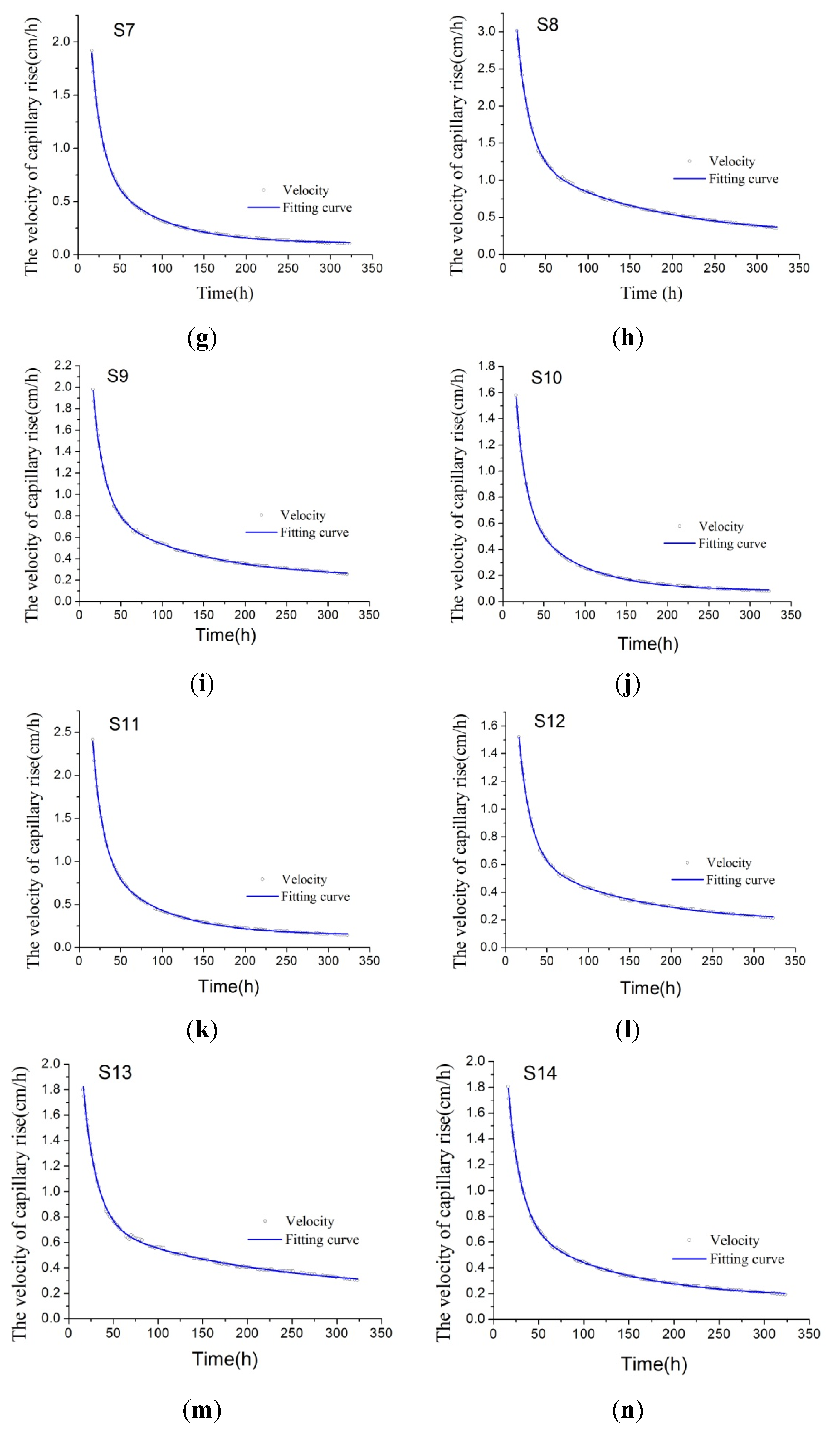
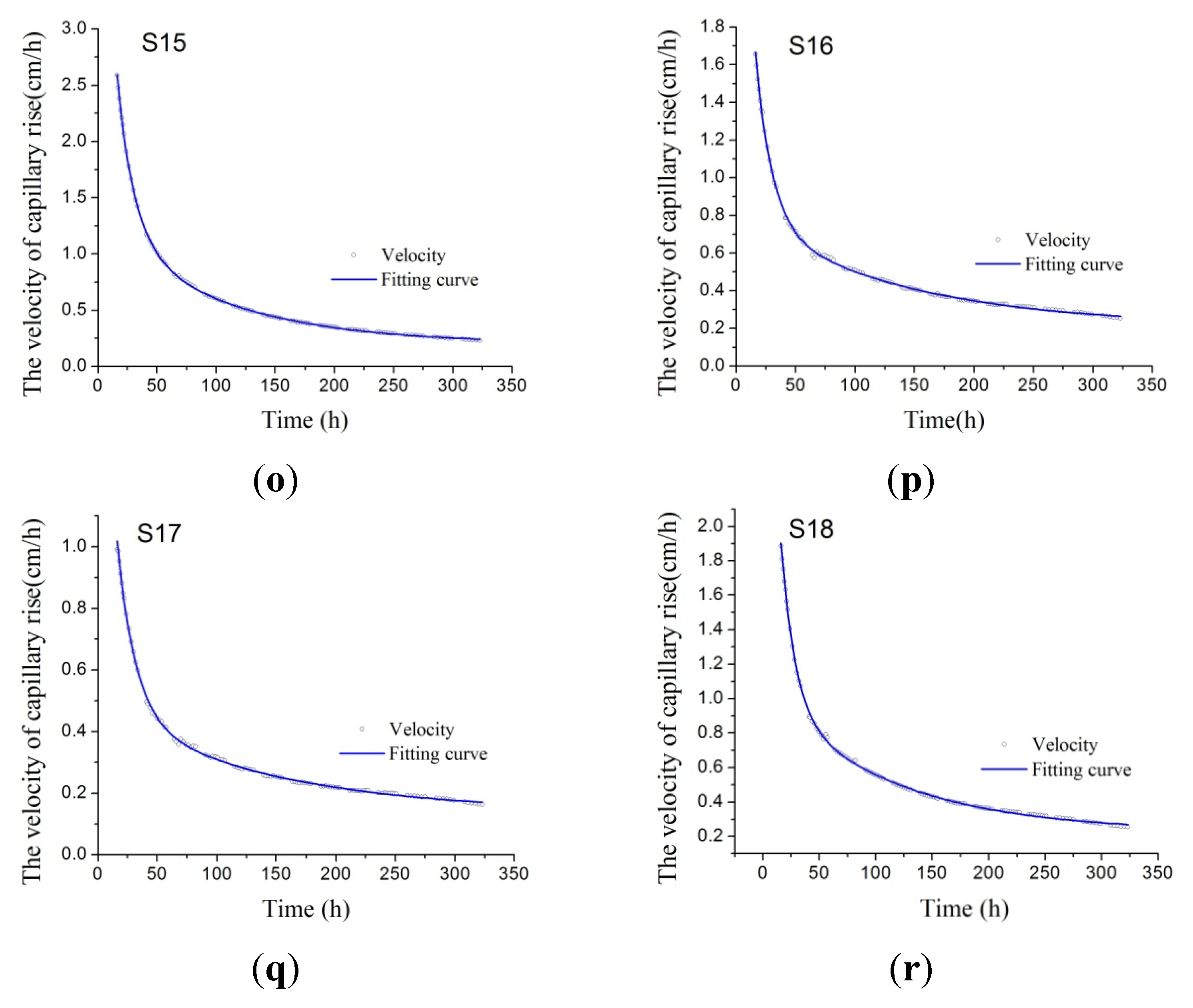
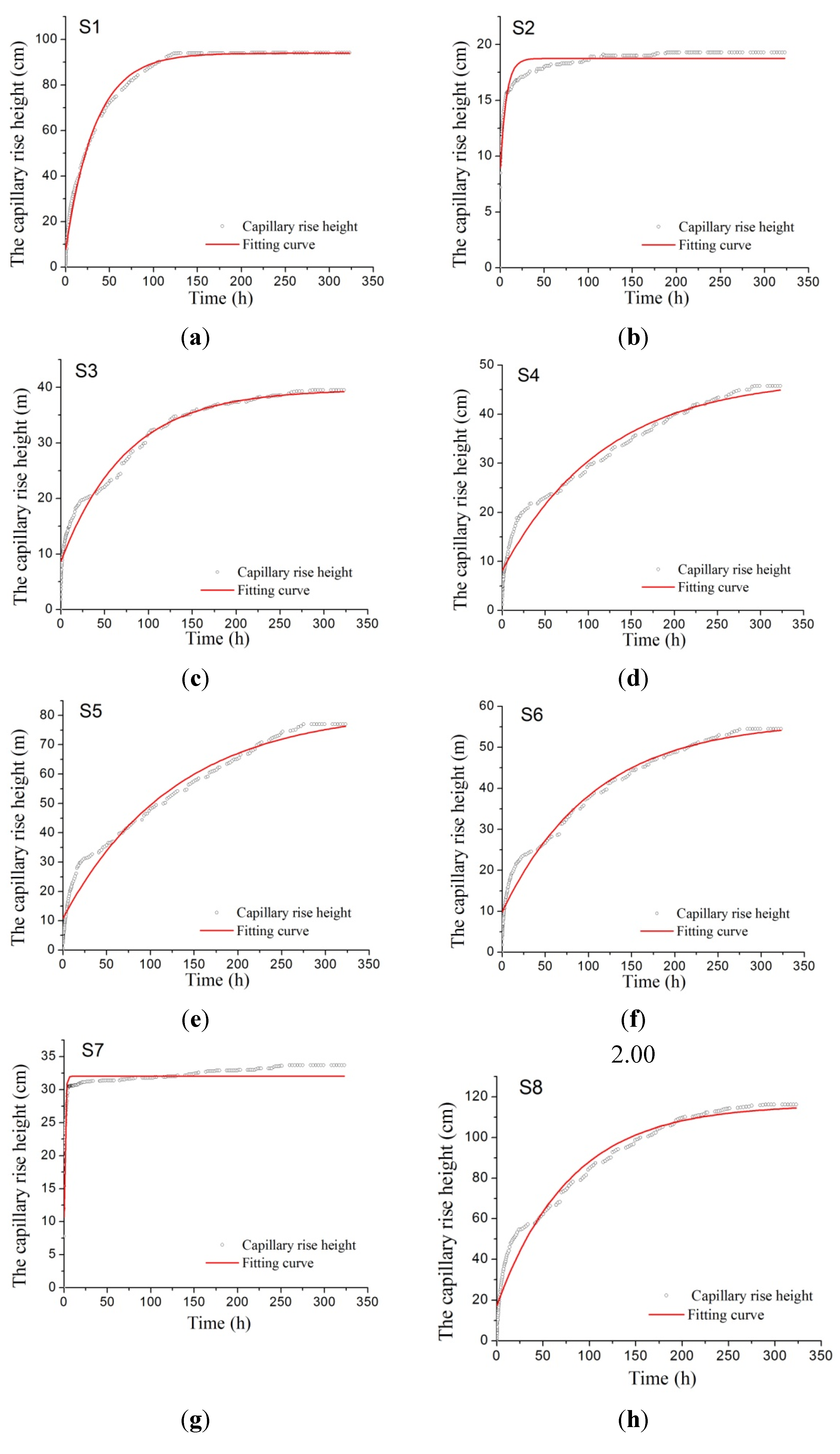
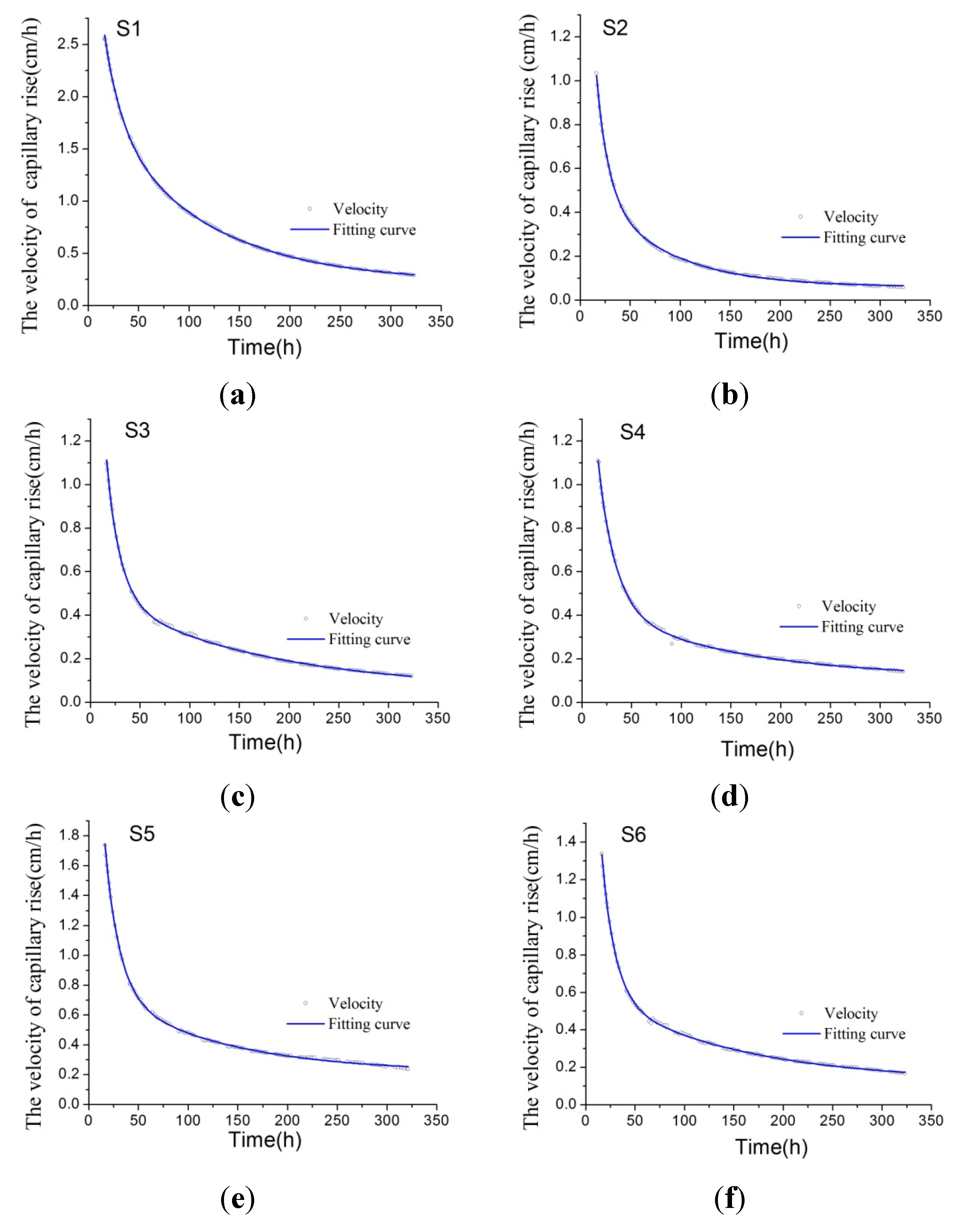
| Sites | Functions | Fitting Curve | R² | CRHP(m) |
|---|---|---|---|---|
| S1 | h-t | y = 14.153ln(x) + 13.978 | 0.9051 | 1.8 |
| v-t | y = 27.082x −0.764 | 0.9825 | ||
| S2 | h-t | y = 1.42ln(x) + 11.898 | 0.9744 | 0.5 |
| v-t | y = 12.976x−0.924 | 0.9995 | ||
| S3 | h-t | y = 5.0915ln(x) + 7.6914 | 0.8948 | 0.6 |
| v-t | y = 7.3382x−0.696 | 0.9930 | ||
| S4 | h-t | y = 5.7629ln(x) + 5.8171 | 0.8591 | 0.7 |
| v-t | y = 6.2311x−0.655 | 0.9921 | ||
| S5 | h-t | y = 10.105ln(x) + 6.7279 | 0.8477 | 1.2 |
| v-t | y = 8.5344x −0.617 | 0.9913 | ||
| S6 | h-t | y = 7.3208ln(x) + 6.3176 | 0.8893 | 0.9 |
| v-t | y = 7.1143x−0.64 | 0.9941 | ||
| S7 | h-t | y = 1.9782ln(x) + 23.331 | 0.8062 | 1.1 |
| v-t | y = 27.691x−0.967 | 0.9999 | ||
| S8 | h-t | y = 16.815ln(x) + 10.936 | 0.9167 | 0.7 |
| v-t | y = 18.127x−0.668 | 0.9956 | ||
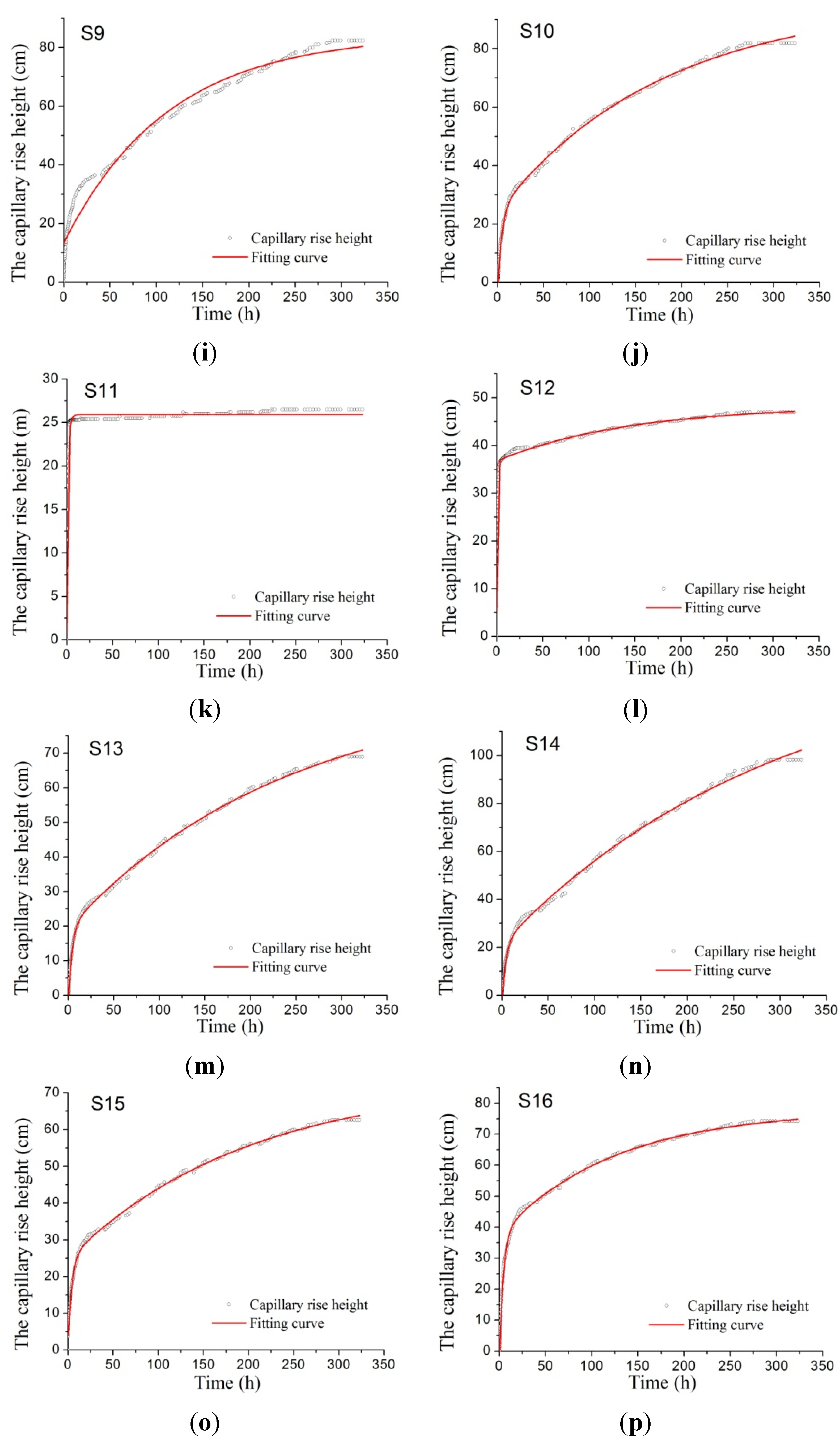
| S9 | h-t | y = 11.108ln(x) + 7.3621 | 0.8959 | 1.4 |
| v-t | y = 11.794ln(x) + 5.068 | 0.9003 | ||
| S10 | h-t | y = 10.085x−0.63 | 0.9967 | 1.1 |
| v-t | y = 10.372x−0.639 | 0.9943 | ||
| S11 | h-t | y = 1.3546ln(x) + 19.87 | 0.9410 | 0.5 |
| v-t | y = 23.749x−0.981 | 0.9999 | ||
| S12 | h-t | y = 3.4666ln(x) + 27.556 | 0.9055 | 0.5 |
| v-t | y = 30.547x−0.926 | 0.9997 | ||
| S13 | h-t | y = 9.5032ln(x) + 4.1629 | 0.8833 | 1.2 |
| v-t | y = 7.3138x−0.609 | 0.9928 | ||
| S14 | h-t | y = 13.531ln(x) + 2.4436 | 0.8414 | 1.4 |
| v-t | y = 6.9448x−0.539 | 0.9829 | ||
| S15 | h-t | y = 8.1193ln(x) + 9.6878 | 0.9263 | 0.6 |
| v-t | y = 11.793x−0.709 | 0.9966 | ||
| S16 | h-t | y = 10.402ln(x) + 12.814 | 0.9696 | 1.2 |
| v-t | y = 23.37x−0.795 | 0.9994 | ||
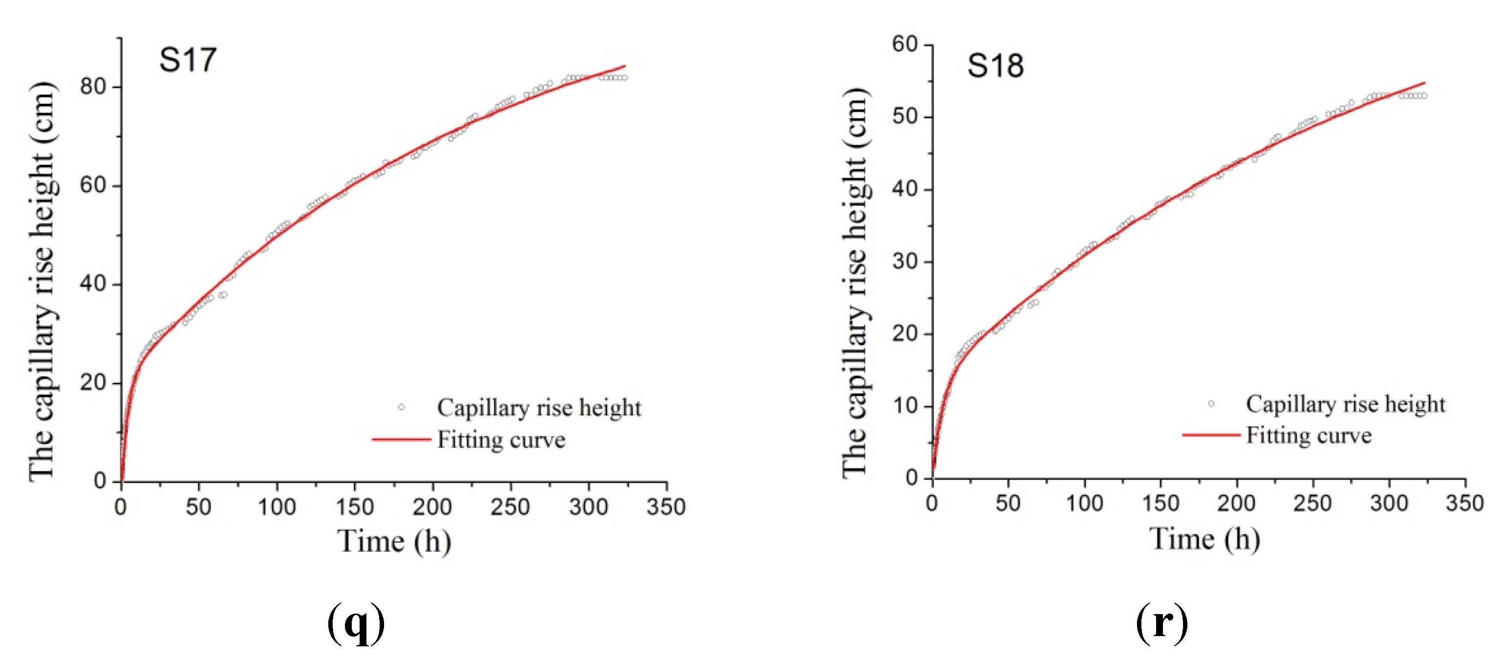
| S17 | h-t | y = 11.271ln(x) + 4.0682 | 0.8676 | 0.5 |
| v-t | y = 7.3882x−0.58 | 0.9922 | ||
| S18 | h-t | y = 7.2199ln(x) + 1.981 | 0.8466 | 0.9 |
| v-t | y = 4.384x−0.568 | 0.9902 |

| Site | Land-Use Type | CRHP (m) | Plant Rooting Depth (m) | The Lower of EISGD (m) | Mean (m) |
|---|---|---|---|---|---|
| S1 | corn | 1.6 | 0.4 | 2.0 | 1.6 |
| S3 | corn | 0.6 | 0.4 | 1.0 | |
| S9 | corn | 1.4 | 0.4 | 1.8 | |
| S16 | corn | 1.2 | 0.4 | 1.6 | |
| S2 | wetland | 0.5 | - | 0.5 | 0.8 |
| S5 | wetland | 1.2 | - | 1.2 | |
| S6 | wetland | 0.9 | - | 0.9 | |
| S11 | wetland | 0.5 | - | 0.5 | |
| S18 | wetland | 0.9 | - | 0.9 | |
| S7 | meadow | 0.4 | 0.4 | 0.8 | 1.2 |
| S10 | meadow | 1.4 | 0.4 | 1.8 | |
| S12 | meadow | 0.6 | 0.4 | 1.0 | |
| S4 | rice | 0.7 | 0.2 | 0.9 | 1.3 |
| S13 | rice | 1.2 | 0.2 | 1.4 | |
| S14 | rice | 1.4 | 0.2 | 1.6 | |
| S8 | woodland | 0.8 | 2 | 2.8 | 2.6 |
| S15 | woodland | 0.6 | 2 | 2.6 | |
| S17 | woodland | 0.4 | 2 | 2.4 |
4.2. Suitable Regions Distribution and Allowable Withdrawal Shallow Groundwater (AWG)
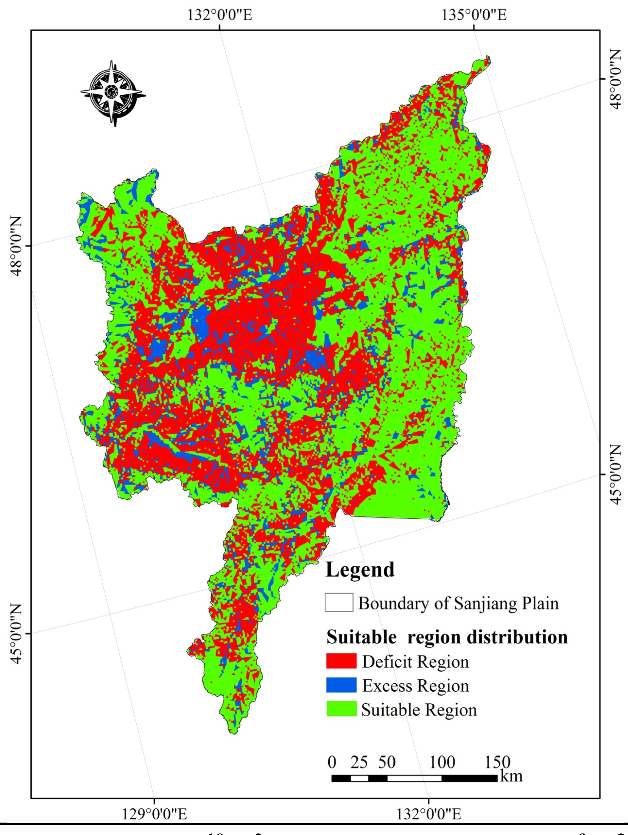
| No. | Name | Area/1010 m2 | Percentage/% | WG/108 m3 | AWG*/108 m3 |
|---|---|---|---|---|---|
| 1 | Excess Region | 1.22 | 11.2 | 7.32 | |
| 2 | Suitable Region | 7.14 | 65.5 | 47.12 | |
| 3 | Deficit Region | 2.54 | 23.3 | −9.14 | 45.3 |
5. Discussion
6. Conclusions
Acknowledgments
Author Contributions
Conflicts of Interest
References
- Quinn, P.; Beven, K.; Culf, A. The introduction of macroscale hydrological complexity into land surface-atmosphere transfer models and the effect on planetary boundary layer development. J. Hydrol. 1995, 166, 421–444. [Google Scholar] [CrossRef]
- York, J.P.; Person, M.; Gutowski, W.J.; Winter, T.C. Putting aquifers into atmospheric simulation models: An example from the Mill Creek Watershed, Northeastern Kansas. Adv. Water Resour. 2002, 25, 221–238. [Google Scholar] [CrossRef]
- Yeh, P.J.F.; Eltahir, E.A. Representation of water table dynamics in a land surface scheme. Part I: Model development. J. Clim. 2005, 18, 38–56. [Google Scholar] [CrossRef]
- Doble, R.; Simmons, C.; Jolly, I.; Walker, G. Spatial relationships between vegetation cover and irrigation-induced groundwater discharge on a semi-arid floodplain, Australia. J. Hydrol. 2006, 329, 75–97. [Google Scholar] [CrossRef]
- Kollet, S.J.; Maxwell, R.M. Capturing the influence of groundwater dynamics on land surface processes using an integrated, distributed watershed model. Water Resour. Res. 2008, 44. [Google Scholar] [CrossRef]
- Zhu, J.; Yu, J.; Wang, P.; Yu, Q.; Eamus, D. Variability in groundwater depth and composition and their impacts on vegetation succession in the lower Heihe River Basin, North-western China. Mar. Freshw. Res. 2013, 65, 206–217. [Google Scholar] [CrossRef]
- Kelliher, F.M.; Kirkham, M.B.; Tauer, C.G. Stomatal resistance, transpiration, and growth of drought-stressed eastern cottonwood. Can. J. For. Res. 1980, 10, 447–451. [Google Scholar] [CrossRef]
- Brothers, T.S. Historical vegetation change in the Owens River riparian woodland. Calif. Riparian Syst. 1984, 15, 75–84. [Google Scholar]
- Kranjcec, J.; Mahoney, J.M.; Rood, S.B. The responses of three riparian cottonwood species to water table decline. For. Ecol. Manag. 1998, 110, 77–87. [Google Scholar] [CrossRef]
- Xu, Y.J.; Burger, J.A.; Aust, W.M. Responses of surface hydrology and early loblolly pine growth to soil disturbance and site preparation in a lower coastal plain wetland. N. Z. J. For. Sci. 2000, 30, 250–265. [Google Scholar]
- Horton, J.L.; Clark, J.L. Water table decline alters growth and survival of Salix gooddingii and Tamarix chinensis seedlings. For. Ecol. Manag. 2001, 140, 239–247. [Google Scholar] [CrossRef]
- Naumburg, E.; Mata-Gonzalez, R.; Hunter, R.G.; Mclendon, T.; Martin, D.W. Phreatophytic vegetation and groundwater fluctuations: A review of current research and application of ecosystem response modeling with an emphasis on Great Basin vegetation. Environ. Manag. 2005, 35, 726–740. [Google Scholar] [CrossRef] [PubMed]
- Fan, Y.; Li, H.; Miguez-Macho, G. Global patterns of groundwater table depth. Science 2013, 339, 940–943. [Google Scholar] [CrossRef] [PubMed]
- Lowry, C.S.; Loheide, S.P.; Moore, C.E.; Lundquist, J.D. Groundwater controls on vegetation composition and patterning in mountain meadows. Water Resour. Res. 2011, 47. [Google Scholar] [CrossRef]
- Satchithanantham, S.; Krahn, V.; Sri, R.R.; Sager, S. Shallow groundwater uptake and irrigation water redistribution within the potato root zone. Agric. Water Manag. 2014, 132, 101–110. [Google Scholar] [CrossRef]
- Schilling, O.S.; Doherty, J.; Kinzelbach, W.; Wang, H.; Yang, P.N.; Brunner, P. Using tree ring data as a proxy for transpiration to reduce predictive uncertainty of a model simulating groundwater-surface water-vegetation interactions. J. Hydrol. 2014, 519, 2258–2271. [Google Scholar] [CrossRef]
- Zhang, C.C.; Shao, J.L.; Li, C.J.; Cui, Y.L. A study on the ecological groundwater table in the North China Plain. J. Jilin Univ. (Earth Sci. Ed.) 2003, 33, 323–326. (In Chinese) [Google Scholar]
- Zhang, X.; Gai, M. Ecological level of groundwater in the Haihe River valley. J. Geol. Hazards Environ. Preserv. 2005, 16, 87–88. (In Chinese) [Google Scholar]
- Sun, X.G.; Ai, X.Y.; Zhang, L.C. The preliminary research on groundwater ecological water table in Sanjiang Plain. Heilongjiang Sci. Technol. Water Conserv. 2012, 40, 166–168. (In Chinese) [Google Scholar]
- Brunner, P.; Li, H.T.; Kinzelbach, W.; Li, W.P. Generating soil electrical conductivity maps at regional level by integrating measurements on the ground and remote sensing data. Int. J. Remote Sens. 2007, 28, 3341–3361. [Google Scholar] [CrossRef]
- Brunner, P.; Li, H.T.; Kinzelbach, W.; Li, W.P.; Dong, X.G. Extracting phreatic evaporation from remotely sensed maps of evapotranspiration. Water Resour. Res. 2008, 44. [Google Scholar] [CrossRef] [Green Version]
- Sun, C.Z.; Gao, Y.; Zhu, Z.R. Estimation of ecological water demands based on ecological water table limitations in the lower reaches of the Liaohe River Plain, China. Acta Ecol. Sinica 2013, 33, 1513–1523. (In Chinese) [Google Scholar]
- Sun, C.Z. Research on the ecological and sustainable groundwater table regulation in the lower Liaohe River plain. J. Jilin Univ. (Earth Sci. Ed.) 2007, 37, 249–254. (In Chinese) [Google Scholar]
- Rong, L.S.; Shu, L.C.; Wang, M.M.; Deng, Z.B. Study on estimation method of ecological water level of reasonable groundwater-case study on lower reaches of the Tarim River. Ground Water 2009, 31, 12–16. (In Chinese) [Google Scholar]
- Xin, X.J.; Xiang, G.S. Study on Reasonable Groundwater Exploitation Based on the Ecological Water Level in Zhangye Basin. Yellow River 2013, 8, 43–48. (In Chinese) [Google Scholar]
- Zhao, Q.; Han, Y.M. Analysis of stimulated recharge of groundwater on the Jiansanjiang Farming Bureau, Sanjiang Plain. J. Heilongjiang Hydraul. Eng. Coll. 2008, 3, 1–4. (In Chinese) [Google Scholar]
- Crosbie, R.S.; Scanlon, B.R.; Mpelasoka, F.S.; Reedy, R.C.; Gates, J.B.; Zhang, L. Potential climate change effects on groundwater recharge in the High Plains Aquifer, USA. Water Resour. Res. 2013, 49, 3936–3951. [Google Scholar] [CrossRef]
- Zeng, R.; Cai, X. Analyzing streamflow changes: Irrigation-enhanced interaction between aquifer and streamflow in the Republican River Basin. Hydrol. Earth Syst. Sci. Discuss. 2014, 10, 7783–7807. [Google Scholar] [CrossRef]
- Herrea-Pantoja, M.; Hiscock, K.M.; Boar, R.R. The potential impact of climate change on groundwater-fed wetlands in Eastern England. Ecohydrology 2012, 5, 401–413. [Google Scholar] [CrossRef]
- Wang, C.Y.; Wu, Z.J.; Shi, Y.L.; Wang, R.Y. The resource of saline soil in the Northeast China. Chin. J. Soil Sci. 2004, 35, 643–646. (In Chinese) [Google Scholar]
- Yang, X.; Yang, W.; Zhang, F.; Chu, Y.; Wang, Y. Investigation and assessment of groundwater resources potential and eco-environment geology in Sanjiang Plain. In China Geology Survey; Geological Publishing House: Beijing, China, 2010. (In Chinese) [Google Scholar]
- Pan, X.F.; Yan, B.X. Effects of land use and changes in cover on the transformation and transportation of iron: A case study of the Sanjiang Plain, Northeast China. Sci. China Earth Sci. 2011, 54, 686–693. [Google Scholar] [CrossRef]
- Wang, X.; Yan, B.X. The Spatial Variation and Factors Controlling the Concentration of Total Dissolved Iron in Rivers, Sanjiang Plain Clean. Soil Air Water 2012, 40, 712–717. [Google Scholar] [CrossRef]
- Cao, Y.J.; Tang, C.Y.; Song, X.F.; Liu, C.M.; Zhang, Y.H. Characteristics of nitrate in major rivers and aquifers of the Sanjiang Plain, China. J. Environ. Monit. 2012, 14. [Google Scholar] [CrossRef] [PubMed]
- Song, K.; Liu, D.; Wang, Z.; Zhang, B.; Jin, C.; Li, F.; Liu, H. Land use change in Sanjiang Plain and its driving forces analysis since 1954. J. Geogr. Sci. 2008, 63, 93–104. [Google Scholar]
- Li, Y.F. Study on the eco-environmental changes in Sanjiang Plain during recent years. Environ. Sci. Manag. 2013, 38, 42–46. [Google Scholar]
- Wang, C.Y.; Wu, Z.J.; Wang, R.Y. Soda-saline soil in the Sanjiang Plain of Heilongjiang Province. Chin. J. Soil Sci. 2001, 32, 23–25. (In Chinese) [Google Scholar]
- Wang, X.; Zhang, G.; Xu, Y.J. Spatiotemporal groundwater recharge estimation for the largest rice production region in Sanjiang Plain, Northeast China. J. Water Supply Res. Technol. 2014, 63, 630–641. [Google Scholar] [CrossRef]
- Drew, M.C.; Stolzy, L.H. Growth under oxygen stress. In Plant Roots: The Hidden Half; Waisel, Y., Eshel, A., Kafkafi, U., Eds.; Marcel Dekker: New York, NY, USA, 1996; pp. 363–381. [Google Scholar]
- Drew, M.C. Oxygen deficiency and root metabolism: Injure and acclimation under hypoxia and anoxia. Annu. Rev. Plant Physiol. 1997, 48, 223–250. [Google Scholar] [CrossRef] [PubMed]
- Sorenson, S.K.; Dileanis, P.D.; Branson, F.A. Soil Water and Vegetation Responses to Precipitation and Changes in Depth to Ground Water in Owens Valley; USGS: Denwer, CA, USA, 1991.
- Rengasamy, P.; Chittleborough, D.; Helyar, K. Root-Zone constraints and plant-based solutions for dryland salinity. Plant Soil 2003, 257, 249–260. [Google Scholar] [CrossRef]
- Bouwer, H. Artificial recharge of groundwater: Hydrogeology and engineering. Hydrogeol. J. 2002, 10, 121–142. [Google Scholar] [CrossRef]
- Lago, M.; Araujo, M. Capillary rise in porous media. J. Colloid Interface Sci. 2001, 234, 35–43. [Google Scholar] [CrossRef] [PubMed]
- Fries, N.; Dreyer, M. The transition from inertial to viscous flow in capillary rise. J. Colloid Interface Sci. 2008, 327, 125–128. [Google Scholar] [CrossRef] [PubMed]
- Averianov, S. Seepage from irrigation canals and its influence on regime of groundwater table. In Influence of Irrigation System on Regime of Ground Water; Academic Press, USSR: Moscow, The Soviet Union, 1956; pp. 140–151. [Google Scholar]
- Chen, T.F.; Wang, X.S.; Li, H.; Jimmy, J.J.; Li, W. Redistribution of groundwater evapotranspiration and water table around a well field in an unconfined aquifer: A simplified analytical model. J. Hydrol. 2013, 495, 162–174. [Google Scholar] [CrossRef]
- Yu, Z.W. The Theory of Crop Planting: North Part; China Agriculture Press: Beijing, China, 2003. (In Chinese) [Google Scholar]
- Ma, W.; Fang, J.; Yang, Y.; Mohammat, A. Biomass carbon stocks and their changes in Northern China’s grasslands during 1982–2006. Sci. China Life Sci. 2010, 53, 841–850. (In Chinese) [Google Scholar] [CrossRef] [PubMed]
- Gardner, W.H. Some steady state solutions of the unsatuarated moisture flow equation with application to evaporation from a water table. Soil Sci. 1950, 85, 228–232. [Google Scholar] [CrossRef]
- Gardner, W.H. Calculation of capillary conductivity from pressure plate outflow date. Soil Sci. Soc. Am. Proc. 1956, 20, 317–320. [Google Scholar] [CrossRef]
- Hillel, D. Introduction to Soil Physics; Academic Press, Inc.: San Diego, CA, USA, 1982; p. 364. [Google Scholar]
- Shah, N.; Nachabe, M.; Ross, M. Extinction depth and evapotranspiration from groundwater under selected land covers. Groundwater 2007, 45, 329–338. [Google Scholar] [CrossRef] [PubMed]
© 2015 by the authors; licensee MDPI, Basel, Switzerland. This article is an open access article distributed under the terms and conditions of the Creative Commons Attribution license (http://creativecommons.org/licenses/by/4.0/).
Share and Cite
Wang, X.; Zhang, G.; Xu, Y.J.; Shan, X. Defining an Ecologically Ideal Shallow Groundwater Depth for Regional Sustainable Management: Conceptual Development and Case Study on the Sanjiang Plain, Northeast China. Water 2015, 7, 3997-4025. https://doi.org/10.3390/w7073997
Wang X, Zhang G, Xu YJ, Shan X. Defining an Ecologically Ideal Shallow Groundwater Depth for Regional Sustainable Management: Conceptual Development and Case Study on the Sanjiang Plain, Northeast China. Water. 2015; 7(7):3997-4025. https://doi.org/10.3390/w7073997
Chicago/Turabian StyleWang, Xihua, Guangxin Zhang, Yi Jun Xu, and Xiangjun Shan. 2015. "Defining an Ecologically Ideal Shallow Groundwater Depth for Regional Sustainable Management: Conceptual Development and Case Study on the Sanjiang Plain, Northeast China" Water 7, no. 7: 3997-4025. https://doi.org/10.3390/w7073997