
Desalination of Water Using ZVI (Fe0)

DCA Consultants Ltd., Haughend, Bridge of Earn Road, Dunning, Perthshire PH2 9BX, UK
Water 2015, 7(7), 3671-3831; https://doi.org/10.3390/w7073671
Submission received: 15 February 2015
/
Revised: 27 May 2015
/
Accepted: 15 June 2015
/
Published: 14 July 2015
Abstract
:Batch treatment of water (0.2 to 240 L) using Fe0 (44,000–77,000 nm) in a diffusion environment operated (at −8 to 25 °C) using: (a) no external energy; (b) pressurized (<0.1 MPa) air; (c) pressurized (<0.1 MPa) acidic gas (CO2); (d) pressurized (<0.1 MPa) anoxic gas (N2); (e) pressurized (<0.1 MPa) anoxic, acidic, reducing gas (H2 + CO + CO2 + CH4 + N2), reduces the salinity of water. Desalination costs increase with increasing NaCl removal. The cost of reducing water salinity from: (i) 2.65 to 1.55 g·L−1 (over 1–24 h) is $0.002–$0.026 m−3; (ii) 38.6 to 0.55 g·L−1 (over 210 days) is $67.6–$187.2 m−3. Desalination is accompanied by the removal, from the water, of one or more of: nitrate, chloride, fluoride, sulphate, phosphate, As, B, Ba, Ca, Cd, Co, Cu, Fe, Mg, Mn, Na, Ni, P, S, Si, Sr, Zn. The rate of desalination is enhanced by increasing temperatures and increasing HCO3−/CO32− concentrations. The rate of desalination decreases with increasing SO42− removal under acidic, or pH neutral, operating conditions.
Keywords:
desalination; zero valent metal; Eh; pH; electrical conductivity (EC); Fe0; Al0; Cu0; FeOOH1. Introduction
Water treatment using zero valent metals (ZVM) in a reactor (or water body) [1,2,3,4,5,6], by aquifer injection/infiltration [7,8,9,10,11,12,13,14], or by placement in a permeable reactive barrier (PRB) located within an aquifer [15,16,17], results in an increase in water pH [5,6,7,18] and a change in water Eh [5,6,7,18]. This is accompanied by a change in water electrical conductivity (EC) [5,6,7,18] which is associated with: (i) the removal of cations and anions from the water by the ZVM (water treatment) [5,6,7,18]; (ii) dissolution of part of the ZVM into the water body [5,19]. Assessment of how the results of this study impact on the removal of microbiota, cations and anions from the water by the ZVM (water treatment) is addressed in Section 6 and Appendix A. ZVM includes Fe0, Cu0, and Al0. In all the trials used in this study, the dominant ZVM is zero valent iron, ZVI (Fe0). The abbreviation ZVI is used for Zero Valent Iron (Fe0).
Analyses of the salinity of water in aquifers passing through PRB’s and in reactors containing ZVM have established that both Na+ and Cl− can be removed from water by ZVM [6,15,20,21,22,23,24,25], or mixtures of ZVM + ion exchange material such as aluminium silicates (e.g., Ca-montmorillonite) [5]. The ZVM is considered to form anodic and cathodic sites in water [18,22,23,24]. The Cl− ions are interpreted as attaching to the anodic sites [22,23]. The iron corrosion rate increases with water velocity [26]. Electrical conductivity (EC) measurements can be used to assess both water salinity and the release of iron corrosion products into the water [20,27].
This study evaluates the partial desalination of water using: (i) 44,000–77,000 nm Fe0 powders which are derived from carbon steel; and (ii) a control/reference air stable 50 nm n-Fe0 powder (PS7) which is impregnated with polyvinylpyrrolidone (PVP) and coated with tetraethylorthosilicate (TEOS) [28].
Na:Fe:C electrochemical capacitor studies have demonstrated that a high capacitance is associated with: (i) structures where a FeIII corrosion product is templated onto Fe0 [29]; (ii) and structures containing a FeIII corrosion product and carbon [29].
1.1. Potential Agricultural Application for Partial Desalination by ZVI
Agricultural water usage for irrigation, livestock and cleaning represents about 70% of global water usage [30] (i.e., about 2600 billion·m3·a−1 [31]). This is projected to rise to between 2800 and 3900 billion·m3·a−1 by 2050 [31]. 260–1000 billion·m3·a−1 of global arable irrigation water is adversely affected by salinity [32,33,34,35]. Any reduction in irrigation water salinity, or livestock feed water salinity, can be expected to result in an increase in crop, or livestock, yield (Appendix B, Figure B1 and Figure B2).
A series of background Figures (Figure B1a–p) have been provided (Appendix B) to show the UN FAO (Food and Agricultural Organization) estimates of the relationship between crop yield and water salinity. This is to demonstrate:
- (1)
- The impact of a decrease in water salinity on the crop yields;
- (2)
- The impact of a small decrease in water salinity on the number of crops which could be grown on an agricultural holding.
For example, a reduction in water salinity from:
- (1)
- 8 to 4 g·L−1 has the potential (Appendix B, Figure B1a) to increase the possible crop yield (t·ha−1) associated with wheat by 300%.
- (2)
- 4 to 2 g·L−1 has the potential (Appendix B, Figure B1i) to increase the possible crop yield (t·ha−1) associated with potato by >200%.
- (3)
- 3 to 1 g·L−1 has the potential (Appendix B, Figure B1g) to increase the possible crop yield (t·ha−1) associated with soft fruit such as blackberry, raspberry or strawberry by >800%.
These changes in crop yield with reduced salinity indicate that if the salinity of saline irrigation water can be reduced for a reasonable cost using a solution that utilises existing reservoirs, impoundments and tanks, then it may be possible to:
- (i)
- Significantly reduce the proportion of global agricultural land which is adversely affected by salinity;
- (ii)
- Increase crop yields on individual agricultural holdings (Appendix B);
- (iii)
- Increase the range of crops that can be grown commercially on a specific agricultural holding (Appendix B).
Irrigation water, supplied as desalinated water produced by large (>100,000 m3·d−1) reverse osmosis (RO), or multistage flash distillation (MSFD) desalination plants, has a delivery cost of US$0.9–3 m−3 [36,37,38].
An agricultural holding may require an irrigation rate of 1000 m3·ha−1·a−1, but may not have access to the finance, or energy, required to operate a suitably sized RO, or MSFD, desalination plant. ZVM desalination has the potential to: (i) reduce the irrigation cost; (ii) utilise existing tanks, ponds and impoundments on the agricultural holding, thereby removing a requirement for new capital investment; (iii) undertake desalination without requiring an energy source (electricity or heat); and (iv) provide an economically viable partial desalination solution for agricultural holdings utilizing 10 to more than 100,000 m3·a−1 of irrigation water.
1.2. Background
1.2.1. Historical ZVI Desalination Experiments
There have been five experimental studies which have evaluated desalination associated with ZVI and ZVM (Fe0 + Al0 + Cu0). They are:
- (1)
- ZVM (Fe0 + Al0 + Cu0)-Ca-montmorillonite combination and ZVI (Fe0)-Ca-montmorillonite. This study [5] demonstrated (Temperature, T = 12–25 °C; Brunauer-Emmett-Teller (BET) surface area, as = 0.00289–0.01732 m2·g−1; ZVI (Fe0) concentration, Pw = 90 g·L−1) (in an open, unstirred, static flow, batch diffusion reactor operated at ambient temperatures) declines in salinity of 25%–50% over 60 days from an initial salinity of about 1 g·L−1.
- (2)
- ZVM (Fe0 and Fe0 + Al0 + Cu0). This study [6] demonstrated (T = 8–20 °C; as = 0.00289–0.01732 m2·g−1; Pw = 90 g·L−1) in an open, unstirred, static flow, batch diffusion reactor operated at ambient temperatures with an initial salinity of about 1 g·L−1, no effective decline in salinity over 60 days.
- (3)
- ZVI (Fe0). This study [20] established (T = 15.3 °C; as = 77.26 m2·g−1; Pw = 3.33 g·L−1) in an open, unstirred, static flow, batch diffusion reactor over 48 h a decline in Cl− concentration from 1.52913 to 1.19831 g·L−1. This was associated with an increase in electrical conductivity (EC) from 3.9 to 4.51 mS·cm−1, and an increase in pH from 6.47 to 9.59.
- (4)
- ZVI (Fe0). This study [21] established (T = 20–22 °C; as = 77.26 m2·g−1; Pw = 8 g·L−1) in an open, continuously stirred, batch diffusion reactor over a 24 h period a statistical relationship between Cl− concentration in the feed water [CF] and product water [CR] over a 24 h period, where CR, mg·L−1 = 1.1 CF0.98 [R2 = 0.99] [21]. The absorbed Cl−, mg·L−1 (CL) = CF − CR.
- (5)
- ZVI (n-Fe0). This study [25] established over a 3 h period using highly reduced n-Fe0, (structured with a Fe0 core and an outer carbon coating (Pw = 1.25 g·L−1; 0.1 gNO3−·L−1), in a fluidised, batch diffusion reactor saturated with argon), a linear relationship between Cl− removal [CL] (g Cl−·g−1 Fe0) and NaCl concentration g·L−1. CL = Adsorbed Cl−, gCl−·g−1 n-Fe0; after 3 h CL = 0.055 g Feed NaCl·L−1. At a salinity of 20 gNaCl·L−1, after 3 h [CL] = 1.1 gCl−·g−1 Fe0. This implies a NaCl removal of 1.77 gNaCl·g−1 Fe0.
These studies establish five important points:
- (1)
- (2)
- (3)
- (4)
- The rate of desalination can be significantly increased by combining ZVM with ion exchange material (e.g., aluminium silicates such as Ca-montmorillonite) [5].
- (5)
1.2.2. ZVI Composition
Most low cost commercial iron powders (<0.1 mm diameter) are constructed from electrolytic iron, or milled iron (44,000–77,000 nm), or iron carbonyl (1000–10,000 nm spheres).
The iron powders will typically contain <0.4 wt % Mn; <0.35 wt % O; <0.03 wt % S; <0.1 wt % Si; <0.04 wt % C; <0.03 wt % P, e.g., [39,40,41,42].
The carbonyl iron will typically contain 0.01–2 wt % C; 0.01–2.5 wt % N, and 0.15–0.5 wt % O [43].
Milled iron produced from carbon steel will have a composition which varies with the grade. For example Q235C/U12358 grade (Chinese Standard GB/T 700-2006 [44]) can contain 0.17 wt % C; 0.35 wt % Si; 1.4 wt % Mn; 0.04 wt % P; 0.04 wt % S; 0.3 wt % Cr; 0.3 wt % Ni; 0.3 wt % Mo; 0.3 wt % Cu, e.g., [45,46].
1.2.3. ZVI Cost
The price of Fe0 powders is a function of particle size, quantity purchased, purity, packaging, stabilization, supplier, and prevailing commodity prices. Indicative FOB (free on board) prices on www.alibaba.com for volume purchases (>10 t) were:
- (i)
- (ii)
- (iii)
The price of small quantities (<5 kg) of chemical grade Fe powders varies with particle size and can fall in the range $50 to greater than$10,000/kg for some powders with a particle size of 1–100 nm (e.g., [47,48,61]).
The term FOB is defined, for international trade, by the Incoterms® 2010 [62,63,64]. The Incoterms® 2010 define FOB as meaning that the seller delivers the goods on board the vessel nominated by the buyer at the named port of shipment, or to a named destination. The risk of loss, or of damage, to the goods passes to the buyer when the goods arrive on board the vessel, or arrive at the nominated destination. The buyer bears all costs from that moment onwards. The Incoterms® 2010 define a number of other alternative international contract structures [62,63,64], which can be applied to the pricing and sale of ZVM powders.
1.2.4. Potential Cost of Partial Desalination Using ZVI
The cost of partial water desalination is a function of: (i) the cost of the ZVI ($·t−1); (ii) the ZVI loading, Pw, g·L−1 (kg·m−3); (iii) length of time required to achieve the required level of desalination; and (iv) the number of times a specific batch of ZVI can be reused.
This study establishes (for a salinity reduction of <4 gNaCl·L−1·d−1), that it is possible to reuse a batch of ZVI at least 18 times. This allows achievement of an effective partial desalination cost for irrigation water of <$0.1 m−3.
1.3. Study Structure
This study includes the results from 137 separate desalination trials and 144 control trials. Trial data, detailed methodology descriptions and background information has been placed in the Appendices in order to improve text readability. The Appendices comprise:
- (a)
- Appendix A: Microbiota, cations, and anions removed by ZVM.
- (b)
- Appendix B: Impact of changing water salinity of arable crop yields and changing feed water salinity on livestock yields;
- (c)
- Appendix C: Trial results: feed and product water cations and anion analyses, gas flow rates, Eh, pH, EC, salinity vs. time, UV-visible spectroscopy analyses of entrained particles.
- (d)
- Appendix D: ZVM compositional and pre-treatment details; Control Reactor Trials;
- (e)
- Appendix E: Interpretation of salinity from electrical conductivity and UV-visible absorbance data.
- (f)
- Appendix F: Fe, Al, Cu corrosion in saline water; Relationship between EC (salinity) and reaction kinetics;
- (g)
- Appendix G: Corrosion species involved in desalination;
- (h)
- Appendix H: Identification of radicals removed during desalination;
Reference to a specific figure or table in an Appendix is prefixed by the Appendix letter, e.g., Figure C1 is located in Appendix C.
1.3.1. ZVM TP and ZVM TPA
This study examines if it is possible to:
- Treat the iron powders (and ZVM combinations) prior to use to form air stable, attrition resistant porous pellets which can partially desalinate water over a 30–250 day trial period. This treated ZVM is termed ZVM TP in this study; TP = treatment product;
- Use a combination of untreated Fe0 and potassium aluminium silicate powder (K-feldspar) to force partial desalination to occur with a 1–24 h period. This combination of untreated Fe0 + K-feldspar is termed ZVM TPA in this study; TPA = treatment product, Type A.
The desalination results associated with:
- The ZVM TP are provided in Section 4 and Section 6, Appendix C (Table C1, Table C2, Table C3 and Table C4; Figure C1, Figure C2, Figure C3, Figure C4, Figure C5, Figure C6, Figure C7, Figure C8, Figure C9, Figure C10, Figure C11, Figure C12, Figure C13, Figure C14, Figure C15, Figure C16, Figure C17 and Figure C18), Appendix D (Figure D1, Figure D2, Figure D3, Figure D4, Figure D5 and Figure D6), Appendix F.
- The ZVM TPA are provided in Section 5, Appendix C (Table C5, Table C6, Table C7, Table C8, Table C9, Table C10, Table C11, Table C12 and Table C13; Figure C19, Figure C20, Figure C21, Figure C22, Figure C23, Figure C24, Figure C25, Figure C26, Figure C27, Figure C28, Figure C29, Figure C30, Figure C31, Figure C32, Figure C33, Figure C34, Figure C35, Figure C36 and Figure C37), Appendix H.
1.3.2. Partial Desalination Information Provided in This Study
- Control Trials and Reference Data (Section 2, Table C1, Table C2, Table C3 and Table C4, Figure D1)
- Natural spring water used to construct the synthetic saline water used in the trials;
- Initial Control Data Set: Variation in Eh, pH, EC of untreated ZVM (Fe0, Al0, Fe0 + Al0, Fe0 + Cu0, Fe0 + Al0 + Cu0) in fresh water and saline water;
- Trial Control Data Set: Variation in Eh, pH, EC of treated particulate ZVM TP (P1) in fresh water (P1c) and saline water (P1);
- Saline feed water used in the trials, at the trial onset and trail conclusion;
- ZVM TP (Section 4 and Section 6, Table C1, Table C2, Table C3 and Table C4; Figure C1, Figure C2, Figure C3, Figure C4, Figure C5, Figure C6, Figure C7, Figure C8, Figure C9, Figure C10, Figure C11, Figure C12, Figure C13, Figure C14, Figure C15, Figure C16, Figure C17 and Figure C18, Table D1 and Table D2, Figure D1, Figure D2, Figure D3, Figure D4, Figure D5 and Figure D6)
- Impact of ZVM pre-treatment on desalination rates;
- Variation in EC (salinity) with time;
- Variation in Eh and pH with time;
- Relationship between desalination and ZVM TP loading (g·L−1);
- Relationship between desalination, particle size and capacitance;
- Economics of partial desalination using ZVM TP.
- ZVM TPA (Section 5, Table C5, Table C6, Table C7, Table C8, Table C9, Table C10, Table C11, Table C12 and Table C13, Figure C19, Figure C20, Figure C21, Figure C22, Figure C23, Figure C24, Figure C25, Figure C26, Figure C27, Figure C28, Figure C29, Figure C30, Figure C31, Figure C32, Figure C33, Figure C34, Figure C35, Figure C36 and Figure C37, Table D3)
- Relationship between desalination rate, ZVM TPA reuse, and time;
- Economics of partial desalination.
- Mechanism of desalination (Section 4 and Section 5, Appendix F, Appendix G, Appendix H)
- Removal of NaCl by incorporation into Fe corrosion products;
- Removal of NaCl by inclusion in a hydration shell;
2. Materials, Methods and Equipment
Tabulated and graphical experimental/trial data used in this study are provided in Appendix C (Table C1, Table C2, Table C3, Table C4, Table C5, Table C6, Table C7, Table C8, Table C9, Table C10, Table C11, Table C12 and Table C13; Figure C1, Figure C2, Figure C3, Figure C4, Figure C5, Figure C6, Figure C7, Figure C8, Figure C9, Figure C10, Figure C11, Figure C12, Figure C13, Figure C14, Figure C15, Figure C16, Figure C17, Figure C18, Figure C19, Figure C20, Figure C21, Figure C22, Figure C23, Figure C24, Figure C25, Figure C26, Figure C27, Figure C28, Figure C29, Figure C30, Figure C31, Figure C32, Figure C33, Figure C34, Figure C35, Figure C36 and Figure C37). All particles used to construct the ZVM TP and ZVM TPA were powdered (44,000–77,000 nm particle size). Details of the ZVM TP and ZVM TPA compositions are provided in Appendix D (Table D1, Table D2 and Table D3).
2.1. Feed Water
The natural untreated spring water used in the trials was extracted from a well located in fractured andesites and acid (rhyolitic) pyroclastics (Devonian, Old Red Sandstone Volcanic Series, Ochil Hills, Scotland). This water has previously been used in ZVM studies [5,6]. The variation in EC, Eh, and pH with time of this water source is documented elsewhere [6]. The cation and anion composition of the natural spring water water is provided in Table C1, Table C2, Table C3 and Table C4. The term freshwater in this study is used to refer to this natural spring water.
2.2. Equipment
Eh, pH, EC, and temperature were measured using equipment manufactured or branded by Hanna Instruments Ltd. (Leighton Buzzard, Bedfordshire LU7 4AD, UK), Extech Instruments (Nashua, NH, USA), HM-Digital Inc. (Culver City, CA, USA) and Oakton Instruments (Vernon Hills, IL, USA). EC, Eh and pH calibration standards used were manufactured or branded by Hanna Instruments, HM-Digital, Milwaukee Instruments Inc. (Rocky Mount, NC, USA). Eh is calibrated to the standard hydrogen electrode (SHE) (Appendix D2.1). Current, voltage, resistance and capacitance of the ZVM TP were measured using equipment manufactured or branded by Philex Electronic (UK) Ltd. (Bedford, UK). Cation and anion analyses were contracted to Forest Research (Farnham, Surrey, UK), the commercial laboratories of the UK Forestry Commission. Anions were determined using Dionex Ion Chromatography (Thermo Fischer Scientific Inc. (Waltham, MA, USA)). Cations were determined using a Thermo Icap 6500 Spectrometer.
Real time salinity changes were determined using EC (Figure C1, Figure C2, Figure C3, Figure C4, Figure C5, Figure C6, Figure C7, Figure C8, Figure C9, Figure C10, Figure C11, Figure C12, Figure C13, Figure C14, Figure C15, Figure C16 and Figure C17 and Figure D1, Figure D2, Figure D3, Figure D4, Figure D5 and Figure D6) and UV-visible spectroscopy (Figure C19, Figure C20, Figure C21, Figure C22, Figure C23, Figure C24, Figure C25, Figure C26, Figure C27, Figure C28, Figure C29, Figure C30, Figure C31, Figure C32, Figure C33, Figure C34, Figure C35 and Figure C36) analysed using a YXUV-5200 spectrometer supplied by Shanghai Selon Scientific Instruments, Shanghai University National Science Park, Shanghai, China. The gas compositions (CH4, CO, CO2, N2, H2) entering and leaving the water from the 3.5 L, 5.4 L and 8 L capacity reactors were monitored using a SRI 8610C TCD GC (manufactured by SRI Instruments Inc. (Torrance, CA, USA)) with a silica gel column and He carrier gas. GC = gas chromatograph, TCD = Thermal Conductivity Detector). Gases and gas calibration standards used in this study were purchased from BOC/Linde, (Guildford, Surrey, UK).
2.3. Control and Reference Trials
2.3.1. Reference Trials: Feedwater Analysed at the Start and End of Each Trial
The trials used saline water which was constructed by either dissolving NaCl into natural spring water (control trials and ZVM TP trials), or by dissolving halite into natural spring water (ZVM TPA trials). Cation and anion compositions are provided in Table C1, Table C2, Table C3 and Table C4 for the saline feed water constructed using NaCl. The amount (wt) of NaCl/halite dissolved into the water was recorded.
The EC, Eh, pH and temperature of the saline water was determined prior to each trail. Some of the saline feed water used in each trial was stored as a control. At the conclusion of the trial the EC, pH and temperature of the saline feed water was redetermined. In each instance the redetermined pH reading was within 0.1 units of the original reading and the redetermined EC reading was within 2% of the original reading. The redetermined results are within the margins of error of the analytical tools used. The reference trials establish that any differences in pH and EC between the original feed water and the product water containing ZVM, or ZVM TP, or ZVM TPA, arise from the presence of the ZVM, ZVM TP and ZVM TPA.
2.3.2. Initial Control Trials Using Untreated ZVM
A series of batch reactors were constructed where each reactor contained ZVM powders (Fe0, Al0, Fe0 + Al0, Fe0 + Cu0 and Fe0 + Al0 + Cu0) + water. Each reactor was not sealed, was open to the air and had an air-water contact. The water was not stirred and the principal interaction between the water and ZVM was by diffusion. These control trials are documented in [6]. Two of the trials (containing Fe0 and Fe0 + Al0 + Cu0) were undertaken in both saline water and freshwater [6] to identify the differences which arise with time in Eh, pH and EC. The EC declines recorded over 60 days in the freshwater and saline water were similar [6]. Therefore it is reasonable to conclude that no noticeable desalination had occurred during the trials with untreated ZVM.
In order to allow comparison with the earlier trials documented in references [5,6], the untreated Fe0, Al0, and Cu0 powders used (and illustrated [5]) in references [5,6] were used to construct the ZVM TP (containing treated ZVM) and ZVM TPA (containing a mixture of untreated ZVM and ion exchange material). The ZVM TPA operating procedure effectively treats the ZVM during desalination.
2.3.3. Control Trial Using ZVM TP
A control trial was established where two trials were run simultaneously (PS1 (Figure C1) and PS1C (Figure D1)) under the same temperature and pressure conditions. In each trial the ZVM TP powder was placed in an unsealed, unstirred, reactor containing a batch of water, and an air-water contact. Reactor PS1 contained saline water. Reactor PS1C contained fresh water. Both Reactors displayed a rapid increase in pH with time (Figure D1), and an initial decrease in Eh followed by a rise in Eh (Figure D1). PS1 displayed a general decrease in EC with time due to desalination (Figure D1), while PS1C displayed a general increase in EC with time due to the release of Fen+ (aq) ions (Figure D1). Water consumption in PS1C was higher than in PS1. 35% of the feed water was consumed in PS1C within 42 days.
Cross plots of Eh vs. pH, Eh vs. EC, and pH vs. EC (Figure D1) indicate that PS1C had a consistently higher pH than PS1 and operated with an Eh over a wider range. The pH in PS1 reduced as the salinity reduced towards the pH of the initial feed water. The pH in PS1C remained at elevated levels. The bulk of the salinity reduction in PS1 occurred at Eh > 0 mV. The Eh in PS1 reduced below 0 mV when the EC fell below 3 mS·cm−1 (Figure D1).
The performance (Eh, pH, EC) of PS1C was similar to that observed for untreated ZVM [6].
2.4. ZVM TP Trials
2.4.1. Temperatures and Pressures Used in the ZVM TP Trials and ZVM TP Control Trial
The reactors were all placed in an external environment. The temperatures and pressures used in the ZVM TP trials (Appendix C) and ZVM TP control trials (Figure D1) are provided in Figure 1.
Figure 1.
Diabatic operating conditions. (a) Temperature; (b) Air Pressure. Data Source: Strathallan weather station (www.weatheronline.com). All trials are referenced to Day 1, where Day 1 is 17 July 2012.
Figure 1.
Diabatic operating conditions. (a) Temperature; (b) Air Pressure. Data Source: Strathallan weather station (www.weatheronline.com). All trials are referenced to Day 1, where Day 1 is 17 July 2012.

2.4.2. Manufacture of ZVM TP
ZVM TP particles and pellets were manufactured by placing the raw ZVM in saline water which was saturated with either:
- Type A: [16.79% CH4 + 16.88% H2 + 11.97% CO + 8.33% CO2 + 46.03% N2], Trials: AS1–AS3, PS5; Manufacturing time = 17 days; Manufacturing time for Trial PS15 = 35 Days;
- Type B: [16.79% CH4 + 16.88% H2 + 11.97% CO + 8.33% CO2 + 46.03% N2 for 110 days] followed by [80% N2 + 20% CO2 for 135 days] followed by [100% N2 for 46 days]; Trials: ST1–ST7, AS4–AS6, PS1–PS4, PS1C; Manufacturing time = 291 days; Manufacturing time for Trial PS16 = 65 Days;
- Type C: [N2] Trials: PS8–PS10, ST8, MT1, MT2; Manufacturing time = 34 days;
- Type D: [air] Trials: PS11, PS12, PS13, MT3, MT4; Manufacturing time = 42 days.
During the manufacturing process the ZVM was maintained at a temperature which varied within the range −8 to 25 °C, and at a pressure which was between atmospheric pressure and 0.1 MPa.
2.4.3. ZVM Composition Used to Manufacture ZVM TP (Table D1 and Table D2)
The molar ZVM compositions entered into the manufacturing reactor to construct the ZVM TP are referenced to Fe0. The recovered ZVM TP was used as particulate matter (Figure 2) or was placed in the water as either:
- (i)
- Copper sheathed pellets (Figure 2),
- (ii)
- MDPE sheathed pellets,
- (iii)
- A cartridge.
Figure 2.
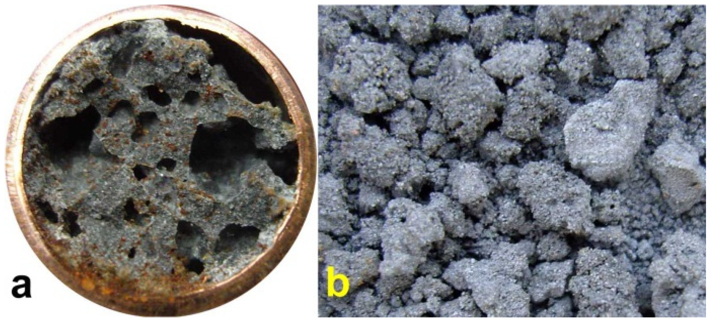
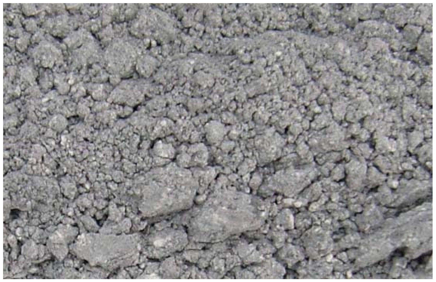
Macroporous ZVM TP (a) End view of a partially oxidized Cu sheathed ST1a–ST5j series ZVM TP pellet (15 mm OD; OD = Outer diameter). Porosity produced by degassing during manufacture; (b) Particulate ZVM TP (PS1–PS4, PS1C, PS15, PS16), field of view = 2 cm.
Figure 2.
Macroporous ZVM TP (a) End view of a partially oxidized Cu sheathed ST1a–ST5j series ZVM TP pellet (15 mm OD; OD = Outer diameter). Porosity produced by degassing during manufacture; (b) Particulate ZVM TP (PS1–PS4, PS1C, PS15, PS16), field of view = 2 cm.
2.4.4. Reactors: ZVM TP Tests at Ambient Temperatures
The reactors used for testing the ZVM TP pellets and particles were containers with capacities of 0.3, 2.3 and 10 L. Each container had an air-water contact and was operated at atmospheric pressure and temperature (Figure 1). The ZVM TP was placed in the reactors and settled at their base. The water in the reactors was not stirred or agitated during the desalination. The upper surface of the reactor was not sealed. This allowed fresh air to continually interact with the water body.
2.4.5. Reactors: ZVM TP Tests Using Pressured Reactors where a Gas Is Used to Maintain the Pressure
Sealed reactors (3.5 and 8 L) containing particulate ZVM TP held in a cartridge, were used for ZVM TP trials CSD1 (8 L reactor), PS15, and PS16. Trials PS15 and PS16 used a reactor with a capacity of 3.5 L. Both reactors had a 1.5 m water column above the gas distributor with >0.5 m gas located above the gas-water contact. The ZVM TP cartridges were located below the gas distributors.
The 8.0 L reactor contained a heat exchanger which allowed the water temperature to be increased into the range 30 to 70 °C.
2.5. ZVM TPA Trials
2.5.1. Cartridge and Particle Manufacture: ZVM TPA (Table D3)
The ZVM TPA was constructed by mixing untreated ZVM with ion exchange material (Figure 3) prior to placement in cartridges. This series of tests determined if this ZVM combination could partially desalinate water over a 1 h to 24 h period, and whether a specific batch of ZVM TP could be used multiple times without regeneration.
2.5.2. Reactors: Used for Testing ZVM TPA
The reactors used for testing the ZVM TPA cartridges had capacities of 5.4, 8.0, 114 and 240 L. Each reactor contained a ZVM TPA cartridge and a gas (80% N2 + 20% CO2, or air) was bubbled through the reactor during operation. The 5.4 and 8.0 L reactors were structured to allow no interaction between air and the gas-water contact in the reactor. The 114 and 240 L reactors were not sealed. They were specifically structured to allow some interaction between atmospheric air and the water body.
3. Interpretation of Salinity
The methodology used to interpret the real time salinity in the trials is detailed in Appendix E, (Figure E1, Figure E2, Figure E3 and Figure E4, Table E1).Two methods are used. They are determination of salinity using EC and determination of salinity using absorbance determined by UV-visible spectroscopy (Figure E1). The basic equations used to calculate salinity are:
(a) Salinity at time t = n calculated using EC:
where [A] = EC due to salinity at time t = 0; [B] = EC due to other components in the water at time t = 0; [C] = EC added to the water by the ZVM, ZVM TP, ZVM TPA between time, t = 0 and time, t = n; [D] = EC due to salinity which has been removed from the water between time, t = 0 and time, t = n; [E] = EC due to other components in the feed water which has been removed from the water between time, t = 0 and time, t = n.
ECt=n = [A] + [B] + [C] − [D] − [E]
EC is related to salinity (Appendix E, Figure E3) using a regression equation of the form:
a and b are constants where b is a function of [B]. a is feed water specific and may vary with temperature.
Salinity = a[EC] + b
(b) Salinity at time t = n calculated using Absorbance at wavelength x nm
where [A]a = Absorbance due to salinity at time t = 0; [B]a = Absorbance due to other components in the water at time t = 0; [C]a = Absorbance added to the water by the ZVM, ZVM TP, ZVM TPA between time, t = 0 and time, t = n; [D]a = Absorbance due to salinity which has been removed from the water between time, t = 0 and time, t = n; [E]a = Absorbance due to other components in the feed water which has been removed from the water between time, t = 0 and time, t = n;
Absorbancet=n = [A]a + [B]a+ [C]a − [D]a − [E]a
Absorbance is related to salinity (Appendix E, Table E1) using a regression equation of the form:
where a, e and f are constants, n is a polynomial number. The regression equation (and applicable equation type, linear, polynomial, etc.) which is applicable will vary with water composition. Different relationships will apply at different wavelengths. Measurement accuracy is enhanced by calculating salinity at multiple wavelengths [65] and then using the average calculated salinity as the salinity of the water [65]. In this study, each salinity value calculated from absorbance is the average of the salinity indicated by 27 different wavelengths (Table E1, Figure E1 and Figure E2). The absorbance attributable to ([A]a − [D]a) is 0 when the salinity is zero.
Salinity = a[absorbance] + b, or Salinity = a[absorbance]n…… e[absorbance] + f
4. Results: ZVM TP
Placement of ZVM TP in a static water body at ambient temperatures, utilising no external energy, established a general decline in salinity with time (Figure C1, Figure C2, Figure C3, Figure C4, Figure C5, Figure C6, Figure C7, Figure C8, Figure C9, Figure C10, Figure C11, Figure C12, Figure C13, Figure C14, Figure C15, Figure C16 and Figure C17). The process produces product water and used ZVM TP. The magnitude of the salinity declines (documented in Table C1, Table C2, Table C3 and Table C4, Figure C1, Figure C2, Figure C3, Figure C4, Figure C5, Figure C6, Figure C7, Figure C8, Figure C9, Figure C10, Figure C11, Figure C12, Figure C13, Figure C14, Figure C15, Figure C16 and Figure C17 and Figure D1, Figure D2, Figure D3, Figure D4, Figure D5 and Figure D6) indicates that ZVM TP pellets or powders have a potential application in the desalination of irrigation water (Appendix B). Salinity declines of up to 8 gNaCl·L−1 are recorded in Figure C1, Figure C2, Figure C3, Figure C4, Figure C5, Figure C6, Figure C7, Figure C8, Figure C9, Figure C10, Figure C11, Figure C12, Figure C13, Figure C14, Figure C15, Figure C16 and Figure C17. Example analyses are summarised in Table 1.
The economic effectiveness of ZVM TP as a potential desalination agent for irrigation water is a function of:
- (1)
- The weight of NaCl removed/unit weight ZVM TP (Qe);
- (2)
- The ZVM TP loading in the water body (weight of ZVM TP/unit volume of water, Pw);
- (3)
- The time, t, taken to achieve the required level of desalination;
- (4)
- The amount of water consumed during desalination;
- (5)
- The number of times the ZVM TP can be reused;
- (6)
- The residual value of the ZVM TP;
- (7)
- The cost of the ZVM TP.
Qe and Pw and the inter-relationship between Qe, Pw, pH, Eh, surface charge, and ZVM TP capacitance are used to assess the economic effectiveness of different pre-treatment methods. The relationship between surface charge/capacitance and EC decline rates is used to provide a measure of quality control for the ZVM TP (i.e., Qe, Pw and the length of time required to achieve a targeted level of desalination).
The significance of Eh, pH, EC, Pw, Qe, temperature, pre-treatment, EC decline rates, and surface charge/capacitance, is discussed here in the context of established Fe corrosion theory in order to demonstrate the mechanism which ZVM TP uses to facilitate desalination and to facilitate the manufacture of more effective ZVM TP desalination pellets and particles.

Table 1.
Changes in water salinity associated with ZVM TP. Gross Qe is calculated from the gross salinity reduction after consideration of water reduction. EC and Salinity Data: Figure C1, Figure C2, Figure C3, Figure C4, Figure C5, Figure C6, Figure C7, Figure C8, Figure C9, Figure C10, Figure C11, Figure C12, Figure C13, Figure C14, Figure C15, Figure C16 and Figure C17; Table C1, Table C2, Table C3 and Table C4. Colour coding reflects the manufacturing process, which is defined in Table D1: Yellow = Type A; Blue = Type B; Tan = Type C; Green = Type D.
| Trial | Feed Water | Feed Water Na + K + Cl | Product Water | Product Water Na + K + Cl | Number of Days | Reduction in Water Volume | Salinity Reduction | EC Reduction | Qe | Gross Salinity Reduction | Gross Qe | ZVM TP |
|---|---|---|---|---|---|---|---|---|---|---|---|---|
| EC mS·cm−1 | mg·L−1 | mS·cm−1 | mg·L−1 | % | mg·L−1 | mS·cm−1 | mg g−1 | mg·L−1 | mg g−1 | g·L−1 | ||
| MT1b | 14.65 | 7,823.30 | 12.53 | 6,614.80 | 100 | 17% | 1,208.50 | 2.12 | 28.1 | 2,359.48 | 54.87 | 43 |
| MT2b | 12.66 | 6,475.88 | 10.93 | 5,922.57 | 98 | 21% | 553.31 | 1.73 | 4.56 | 1,785.20 | 14.72 | 121.3 |
| MT3d | 7.23 | 3,465.60 | 6.46 | 3,308.2 | 98 | 17% | 157.40 | 0.77 | 2.5 | 733.03 | 11.65 | 62.9 |
| MT4d | 7.84 | 3988.07 | 6.57 | 3,149.62 | 57 | 9% | 838.45 | 1.27 | 9.31 | 1,112.47 | 12.35 | 90.1 |
| ST3b | 18.84 | 11,049.49 | 6.73 | 3,374.48 | 126 | 25% | 7,675.01 | 12.11 | 307 | 8,518.63 | 340.75 | 25 |
| ST3f | 18.84 | 11,049.49 | 6.66 | 3,052.11 | 126 | 25% | 7,997.38 | 12.18 | 139.08 | 8,760.41 | 152.35 | 57.5 |
| ST6d | 16.59 | 9,089.82 | 15.74 | 8,550.01 | 120 | 17% | 539.81 | 0.85 | 105.85 | 2,027.51 | 397.55 | 5.1 |
| ST8e | 12.35 | 6,380.24 | 10.95 | 5,814.14 | 98 | 6% | 566.10 | 1.4 | 15.51 | 903.32 | 24.75 | 36.5 |
| PS4 | 19.71 | 10,001.69 | 5.05 | 2,195.88 | 150 | 45% | 7,805.81 | 14.66 | 141.92 | 8,793.96 | 159.89 | 55 |
| PS5 | 15.18 | 7,609.68 | 5.32 | 2,633.33 | 150 | 45% | 4,976.35 | 9.86 | 165.88 | 6,161.35 | 205.38 | 30 |
| PS7 | 14.05 | 7,391.68 | 4.7 | 1,941.37 | 198 | 45% | 5450.30 | 9.35 | 2180.12 | 6,323.93 | 2529.57 | 2.5 |
| PS11 | 7.84 | 3,988.07 | 5.43 | 2,664.32 | 57 | 7% | 1,323.75 | 2.41 | 49.95 | 1,515.58 | 57.19 | 26.5 |
| PS14 | 6.41 | 3,162.04 | 5.66 | 3,024.48 | 57 | 22% | 137.56 | 0.75 | 13.49 | 793.87 | 77.83 | 10.2 |
| PS15 | 57.49 | 23,707.28 | 31.12 | 17,284.81 | 79 | 33% | 6,422.47 | 26.37 | 47.93 | 12,212.88 | 91.14 | 134 |
| PS16 | 78.18 | 38,577.1 | 1.09 | 576.48 | 210 | 74% | 38,000.62 | 77.09 | 182.7 | 38,424.33 | 184.73 | 208 |
The NaCl is removed by the ZVM TP and is not present as a separate precipitate within the water. This demonstrates that the NaCl interacts with, and is bound into, a reaction product associated with the corrosion of ZVM TP in water.
The NaCl is removed by one or more of:
- (1)
- Incorporation into a Fe corrosion product. Green Rust One (Cl−), GR1, incorporates Cl− ions in its crystal structure. β-FeOOH requires the presence of Cl− ions to form. All other Fe corrosion products do not incorporate Cl− ions within their crystal structure. In this instance Qe < 70 mg NaCl removed g−1 ZVM [67,68,69,70,71,72,73,74,75,76,77,78,79,80,81,82,83,84,85,86,87,88,89,90,91,92,93,94,95,96,97,98,99,100].
- (2)
- Incorporation into the hydration shell of a Fe corrosion product (e.g., green rust, FeOOH) [96]. A hydrated amorphous FeOOH corrosion product containing 46 wt % H2O will contain 5 hydration shells. Radicals containing Na+ and Cl− can substitute for H2O in the hydration lattice [96]. This may potentially allow Qe to exceed 3 gNaCl removed g−1 ZVM [96].
- (3)
- Concentration of NaCl in the pore waters within the ZVM TP/ZVM TPA corrosion product bed, when the ZVM interacts with the overlying water body by diffusion. This may potentially allow Qe to exceed 20 gNaCl·removed·g−1 ZVM. This method of NaCl removal is investigated in the ZVM TP trials CSD1 and ZVM TPA trials E143, and E144 (Section 5).
The method of NaCl removal is considered in the context of established iron corrosion theory (Section 4.2).
4.1. Pre-Treatment
The relative effectiveness of a treatment process can be evaluated using a standardized measure of salinity reduction, Qe, (mgNaCl·removed·g−1 ZVM). The relative effectiveness of different pre-treatments (for similar sized ZVM particles) is demonstrated by the data in Table 1 and reference [6] to be:
[H2 + CH4 + CO + CO2 + N2] > [N2] > [air] > no pretreatment
The pre-treatment is designed to increase the amount of NaCl incorporated into the hydration shell of a Fe corrosion product during desalination.
Example Calculation of the Relative Efficiency of a Pre-Treatment: ST1a, MT2b
The rate of decline in salinity is a measure of the size of the facilities required to process a specific volume of water over a specific time period. For example, a reduction in the length of time taken to achieve a reduction of x g·L−1 from 100 days to 20 days, allows:
- The size of the desalination tanks (water bodies) required to be reduced by 80% (e.g., from 1000 to 200 m3);
- The land take required for the desalination tanks to be reduced from 100–500 m2 to 50–150 m2.
The EC declines associated with ZVM TP can be analysed in accordance with the methodology in Section F3, where [at+1] is a normalized measure of the relative efficiency of the desalination process. [at+1] increases with increasing desalination efficiency. This analysis, summarised in Table 2 and Figure 4 for example calculations using ST1a and MT2b, establishes:
- The expected value of [at+1] if the ZVM is used at a specific Pw, without pre-treatment;
- The expected value of [at+1] following pre-treatment without considering water losses;
- The expected value of [at+1] following pre-treatment after consideration of water losses.
This analysis demonstrates the benefit of pre-treatment, and allows the effectiveness of different types of pre-treatment to be evaluated. In this example, a Type B pre-treatment is more effective than a Type C pre-treatment.
Table 2.
Assessed Impact of Pre-Treatment on the desalination rate using [at+1] is an adjustable variable. Data: Figure 4a–d. Reference data set without pre-treatment: [6,21]: as = 0.017 m2·g−1 [6]; Methodology: Appendix F3.
| Trial | Expected without Pre-Treatment | With Pre-Treatment | Adjusted for Water Consumption | Improvement Due to Pre-Treatment | Improvement Due to Pre-Treatment |
|---|---|---|---|---|---|
| Observed | Observed | Adjusted for Water Consumption | |||
| ST1a | 0.00020 | 0.12000 | 0.15000 | 60,000% | 75,000% |
| MT2b | 0.00134 | 0.02000 | 0.10000 | 1498% | 7491% |
The data required to calculate [at+1] is:
- The surface area, as, and Pw of the ZVI used in the reference desalination data set using untreated ZVI (Section 1.2.1 and Section 2.3.2 [21]);
- The as and Pw of the ZVI used in the control desalination data using untreated ZVI (Section 2.3.2 [6]);
- Qe and Pw for the individual trial (Table 1, Figure C1, Figure C2, Figure C3, Figure C4, Figure C5, Figure C6, Figure C7, Figure C8, Figure C9, Figure C10, Figure C11, Figure C12, Figure C13, Figure C14, Figure C15 and Figure C16).
The desalination is associated with changes in Eh (Figure C5 and Figure C14). Changes in Eh reflect changes in the rate of hydrolysis, where decreases in Eh represent increased hydrolysis, and increases in Eh represent reduced hydrolysis [67]. They indicate that NaCl removal is associated with the OH radical and related species (e.g., HO2−) [67]. This is confirmed by the [at+1] analysis in Table 2 where hydrolysis improves the effective NaCl removal efficiency of a Type B pre-treatment by 25%, and a Type C pre-treatment by 500%.
Figure 4.
Example EC changes vs. time. (a) ST1a; (b) MT2b; (c) ST1a, adjusted for water losses; (d) MT2b, adjusted for water losses. Spikes where the EC rises represent periods when the water was partially frozen. Spikes where the EC reduces to zero represent periods when the entire water body was frozen. Data: Figure C5 and Figure C14. Methodology: Appendix F3.

PS14 (Figure F1) used a Type A gaseous pre-treatment (Table D1). A [a + t] analysis (Section F3), normalising the particle size in PS14, to the particle size used in ST1a, and setting a Pw of 20 g·L−1, indicates that PS14 would be expected to provide a Qe of 346 mgNaCl·g−1 ZVM TP. Similar values of Qe are recorded for ST3b (Table 1) which was manufactured using a Type B pre-treatment. The Type A pre-treatment undertaken in a gaseous environment can be as effective as a Type B pre-treatment undertaken in an aqueous environment.
4.2. Iron Corrosion in Saline Water
The removal of NaCl is associated with ZVM TP corrosion. The rate of corrosion, the nature of the ZVM TP corrosion products, and the nature of the Eh and pH environment created by the ZVM TP controls the rate of desalination [18,19,67,68,69,70,71,72,73,74,75,76,77,78,79,80,81,82,83,84,85,86,87,88,89,90,91,92,93,94,95,96,97,98,99,100].
Two roles have been proposed for Cl− during iron corrosion, they are:
Appendix F1, Appendix F2 and Appendix G consider the principal corrosion products associated with ZVM TP and ZVI in the Eh and pH environment created by the ZVM TP (Figure C1, Figure C2, Figure C3, Figure C4, Figure C5, Figure C6, Figure C7, Figure C8, Figure C9, Figure C10, Figure C11, Figure C12, Figure C13, Figure C14, Figure C15 and Figure C16).
4.2.1. Pourbaix Relationships
Eh and pH define the stable (equilibrium) phases of iron which will be present in the pore waters and ZVM TP body [19]. They also define the corrosion sequence that occurs [19]. Analysis of aqueous ion (and ion adduct) equilibrium using temperature, pressure, pH and Eh is termed a Pourbaix analysis [19]. For any aqueous reaction involving one or more of ions, ion adducts (precipitates) and gaseous species, a Pourbaix analysis defines [19] the equilibrium constant, K, the Reaction Quotient, Q, the Gibbs Free Energy, G, the heat of formation, H, and the enthalpy, S, associated with the reaction (Appendix F2). Therefore, if two or more reaction products are theoretically possible a Pourbaix analysis will identify which species is the equilibrium product [19]. A Pourbaix analysis will allow the equilibrium ion concentrations and gas partial pressures to be determined for a specific Eh and pH [19].
Iron, as it corrodes, adjusts the Eh and pH of the water with time [5,6,18]. The initial change is an increase in pH followed by a subsequent decrease in pH [5,6,18]. The Eh either initially drops, or remains stable, before rising and then falling [5,6,18]. These changes are associated with the progressive formation in fresh water of [19]:
Fe0 → Fe(OH)2 → FeOOH
The Eh and pH at any moment in time defines [19] the equibrium constants for Fe(OH)2 and FeOOH. During periods when Eh and pH are constantly changing (e.g., Figure C1, Figure C2, Figure C3, Figure C4, Figure C5, Figure C6, Figure C7, Figure C8, Figure C9, Figure C10, Figure C11, Figure C12, Figure C13, Figure C14, Figure C15, Figure C16 and Figure C17 and Figure C19, Figure C20, Figure C21, Figure C22, Figure C23, Figure C24, Figure C25, Figure C26, Figure C27, Figure C28, Figure C29, Figure C30, Figure C31, Figure C32, Figure C33, Figure C34, Figure C35 and Figure C36) the water is in disequilibria [19]. Once the Eh and pH values achieve a stable level (at a constant temperature and pressure (e.g., Figure C1, Figure C2, Figure C3, Figure C4, Figure C5, Figure C6, Figure C7, Figure C8, Figure C9, Figure C10, Figure C11, Figure C12, Figure C13, Figure C14, Figure C15, Figure C16 and Figure C17 and Figure C19, Figure C20, Figure C21, Figure C22, Figure C23, Figure C24, Figure C25, Figure C26, Figure C27, Figure C28, Figure C29, Figure C30, Figure C31, Figure C32, Figure C33, Figure C34, Figure C35 and Figure C36) the water is in a chemical equilibrium [19].
Eh, pH relationships do not define reaction rates (though the rate of change and direction of change is a reflection of underlying reaction rates) [19]. They do define the equilibrium product species and where two, or more, species can occur, the equilibrium molar ratios between the products [19].
A byproduct of iron corrosion is the removal and consumption of water [19]. Water removal was observed in the trials associated with both ZVM TP and ZVM TPA (Appendix C). The principle reactions are [19]:
Fe0 → Fen+ + ne−
H2O = H+ + OH−
The rate of water ionisation is higher than the rate of iron ionisation [19] and the amount (wt) of water removed can exceed the weight of Fe placed in the reaction environment (e.g., Table 1, Appendix C).
4.2.2. Fe0 Corrosion Series
The established redox (Eh, pH) boundaries for the stable phases of iron [19,69,70,71,72,73,74,75] in saline water are shown in Figure 5a. The stable equilibrium species are Fe0, Fe2+ ions, Fe(OH)2, Green Rust One (GR1, GR:Cl), and FeOOH. During corrosion (oxidation), the sequential reaction series in saline water which is free of sulphates and bicarbonates/carbonates is [19,69,70,71,72,73,74,75]:
Fe0 → Fe(OH)2 → GR1(Cl−) → FeOOH
The GR1 either [43,44,45,46,47,48,49]:
- transforms directly to β-FeOOH (akaganeite), or,
- adopts the reaction series, GR1 → α-FeOOH (goethite) → β-FeOOH, or,
- adopts the reaction series GR1 → γ-FeOOH (lepidocrocite) → α-FeOOH → β-FeOOH
In the presence of sulphate the corrosion reaction series is:
Fe0 → Fe(OH)2 → GR1(Cl−) → GR1(SO32−) → GR2(SO42−) → FeOOH (γ-FeOOH and/or α-FeOOH)
In the presence of carbonate/bicarbonate the corrosion reaction series is:
Fe0 → Fe(OH)2 → GR1(Cl−) → GR1(CO32−) → FeOOH (γ-FeOOH and/or α-FeOOH)
The corrosion of Fe0 in the presence of sulphate, carbonate, and bicarbonate is addressed in Section 6.
The trials analysed in Section 4 and Section 5 were operated in saline water containing <11 mgSO42−·L−1 (Table C1) and <100 mgHCO3−·L−1.
The corrosion of Fe0 to FeOOH produces adsorbed hydrogen (Fe + 2H2O = FeOOH + 3H+ + 3e−) [19]. The adsorbed hydrogen can interact with Fen+ ions at the FeOOH–water boundary to initiate the templated growth of GR1 growing from a FeOOH corroded ZVM particle (Figure F1) [69,70,71,72,73,74,75]:
FeOOH → GR1(Cl−) → FeOOH
Excess H2 (gas) formed as 2H+ + 2e− = H2 [19], can form small trapped accumulations of hydrogen [5,18] within the pore space of the ZVM TP (e.g., Figure F1). This hydrogen interacts with the FeOOH corrosion products to produce Fe3O4 (e.g., Figure F1) [19,83]:
3FeOOH + 0.5H2 → Fe3O4 + 2H2O
The corrosion environment associated with both iron corrosion and desalination is complex and dynamic. The trials documented in Figure C1, Figure C2, Figure C3, Figure C4, Figure C5, Figure C6, Figure C7, Figure C8, Figure C9, Figure C10, Figure C11, Figure C12, Figure C13, Figure C14, Figure C15 and Figure C16 used water which contained trace quantities of sulphates (Table C1) and bicarbonates/carbonates.
Figure 5.
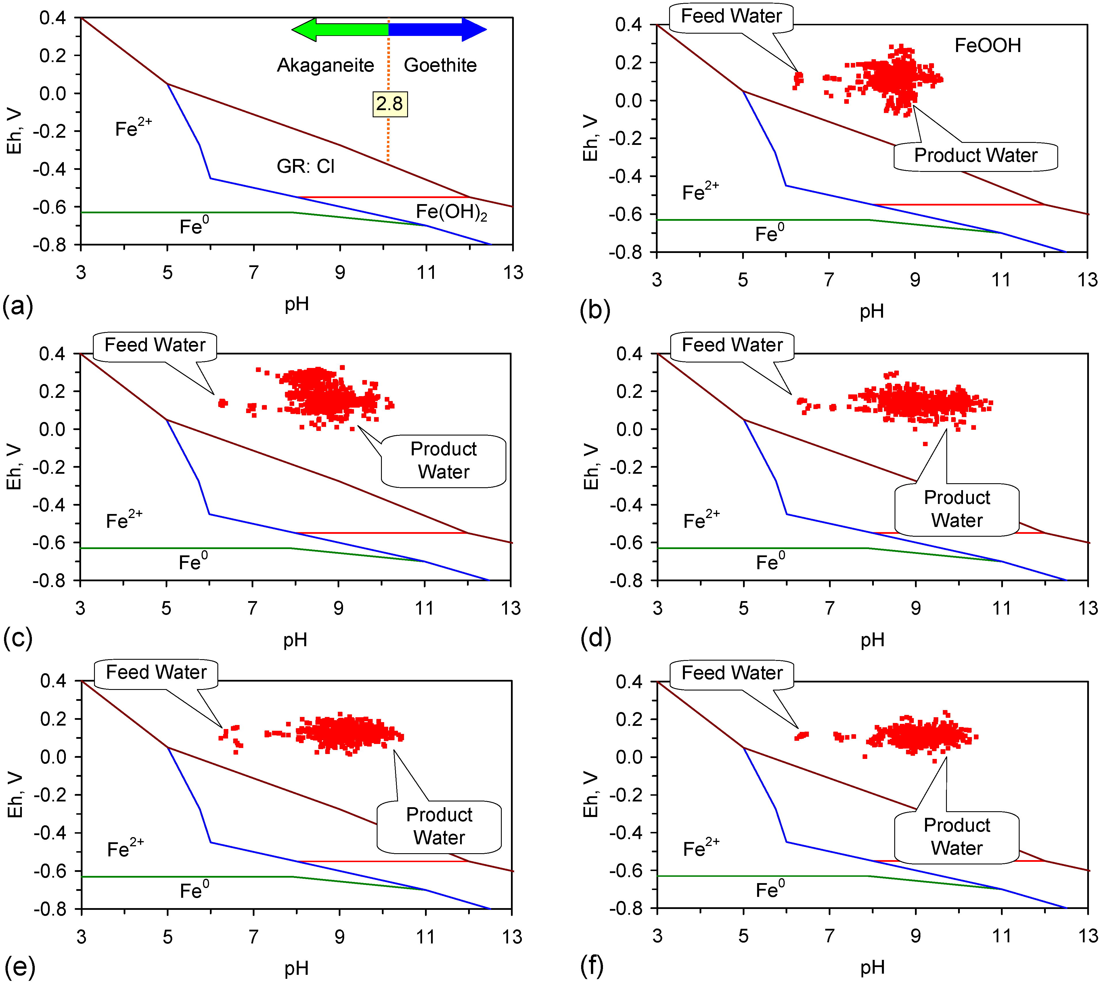
Eh vs. pH for the ST1 to ST5 series of ZVM TP trials (Figure C5, Figure C6, Figure C7, Figure C8 and Figure C9). (a) Pourbaix diagram identifying the dominant Fe species phase as a function of Eh and pH [19,69,70,71,72,73,74,75]. GR = green rust. 2.8 = 2.8 mgCl−·L−1 for R = 8; (b) ST1; (c) ST2; (d) ST3; (e) ST4; (f) ST5. Increasing the concentration of Cl− (salinity) increases the pH required to achieve R = 8, and increases the pH range where akaganeite is the dominant FeOOH corrosion species. Data taken for the time period between the date the ZVM TP was added to the water to the date the partial freezing event identified in Figure C5, Figure C6, Figure C7, Figure C8 and Figure C9. This is to demonstrate the Eh vs. pH redox regime during the principal desalination phase.
Figure 5.
Eh vs. pH for the ST1 to ST5 series of ZVM TP trials (Figure C5, Figure C6, Figure C7, Figure C8 and Figure C9). (a) Pourbaix diagram identifying the dominant Fe species phase as a function of Eh and pH [19,69,70,71,72,73,74,75]. GR = green rust. 2.8 = 2.8 mgCl−·L−1 for R = 8; (b) ST1; (c) ST2; (d) ST3; (e) ST4; (f) ST5. Increasing the concentration of Cl− (salinity) increases the pH required to achieve R = 8, and increases the pH range where akaganeite is the dominant FeOOH corrosion species. Data taken for the time period between the date the ZVM TP was added to the water to the date the partial freezing event identified in Figure C5, Figure C6, Figure C7, Figure C8 and Figure C9. This is to demonstrate the Eh vs. pH redox regime during the principal desalination phase.
4.2.3. Transformation from α-FeOOH → β-FeOOH
The transformation from α-FeOOH → β-FeOOH is a function of the pH and Cl− concentration in the water [69,70,71]. The molar ratio, R, log (Cl−/OH−) in the feed water has been proven to be an accurate predictor of the dominant (equilibrium) precipitated FeOOH species [69,70,71]. These studies have established that when:
- 1
- 2
- 3
- 4
- R ≥ 8, the only equilibrium FeOOH species which will be present is β-FeOOH [71].
The transformation from α-FeOOH → β-FeOOH is not instantaneous, therefore analyses of FeOOH species prior to equilibrium being achieved may show the presence of α-FeOOH.
At a pH of 10, R = 8 corresponds to a Cl− concentration of 2.8 mgCl−·L−1 (4.5 mgNaCl·L−1) (Figure 5a). In all the examples (ZVM TP and ZVM TPA) considered in this study (Figure C1, Figure C2, Figure C3, Figure C4, Figure C5, Figure C6, Figure C7, Figure C8, Figure C9, Figure C10, Figure C11, Figure C12, Figure C13, Figure C14, Figure C15, Figure C16, Figure C17, Figure C19, Figure C20, Figure C21, Figure C22, Figure C23, Figure C24, Figure C25, Figure C26, Figure C27, Figure C28, Figure C29, Figure C30, Figure C31, Figure C32, Figure C33, Figure C34, Figure C35, Figure C36 and Figure D1, Figure D2, Figure D3, Figure D4, Figure D5 and Figure D6), R is greater than 8, when the water pH < 13.
4.2.4. Dominant Corrosion Species Associated with ZVM TP
The Eh vs. pH cross plots (Figure 5) from 50 trials (ST1a to ST5j) indicate that the water chemistry throughout the trials was in the FeOOH precipitation zone [19]. The dominant Fe corrosion product surrounding the Fe0 core will be FeOOH [19]. R > 8, therefore any entrained n-Fe particles will be β-FeOOH [19,69,70,71]. Similar Eh, pH observations were made in the trials documented in Figure C1, Figure C2, Figure C3, Figure C4, Figure C10, Figure C11, Figure C12, Figure C13, Figure C14, Figure C15, Figure C16, Figure C17, Figure C19, Figure C20, Figure C21, Figure C22, Figure C23, Figure C24, Figure C25, Figure C26, Figure C27, Figure C28, Figure C29, Figure C30, Figure C31, Figure C32, Figure C33, Figure C34, Figure C35 and Figure C36.
The corrosion product reaction sequences result in a series of concentric halos of different corrosion products surrounding the Fe0 particle core [68]. Example halos associated with ZVM TP are illustrated in Figure F1. In this example the initial particle corrosion results in a structure where an Fe0 core is surrounded by Fe(OH)2 and the Fe(OH)2 is then surrounded by β-FeOOH (e.g., Figure F1). The β-FeOOH acts as a template for the growth of Schiller sheets of GR1. These are transformed at their margins to β-FeOOH (e.g., Figure F1) [76,77,87,88]. Figure F1 demonstrates the presence of, and growth of, spherulitic, amorphous, entrained particles of β-FeOOH. These particles display the characteristic colour of β-FeOOH (Figure F1). The margins of the Schiller sheets have a purple colour (Figure F1). This colour is a characteristic of Na incorporation in the lattice (see Appendix H).
4.2.5. NaCl Removal in the Hydrated Layers Surrounding ZVM TP
The Pourbaix analysis [19,69,70,71,72,73,74,75] has established that desalination is associated with green rust and FeOOH corrosion species. Figure F1 demonstrates incorporation of Cl− ions into entrained amorphous β-FeOOH and incorporation of Na+ ions into FeIII species associated with growing Schiller sheets within a ZVM TP body. Incorporation into these species is unable to account for the high levels of NaCl removal (e.g., PS14 (Table 1, Figure F1) Qe = 77.83 mg·g−1) observed (Table 1, Figure C1, Figure C2, Figure C3, Figure C4, Figure C5, Figure C6, Figure C7, Figure C8, Figure C9, Figure C10, Figure C11, Figure C12, Figure C13, Figure C14, Figure C15 and Figure C16). The removed NaCl is located principally in the hydration shells associated with ZVM TP and its corrosion products [87,88,96].
The hydrated shells surrounding FeOOH can remove NaCl by adsorption [78,79,80] or by concentration in the pore water within the ZVM body, surrounding the ZVM particles (e.g., Figure D1).
Analysis of ZVM TP will be expected (e.g., Figure F1) to contain a mixture of Fe0, FeII and FeIII species. The entrained FeIII species will be expected to contain a mixture of γ-FeOOH, α-FeOOH, β-FeOOH.
4.2.6. Identification of FeOOH or Other Fe Species Involved in NaCl Removal
Fe corrosion species have been identified from solid material using a number of different techniques including: Raman spectroscopy; X-Ray diffraction (XRD), Differential scanning calorimetry, FTIR, UV-Visible spectroscopy, fluorospectroscopy, vibrating sample magnetometry, electron paramagentic resonance, optical analyses, Mossbauer, Synchron X-ray powder analyses etc. Entrained Fe corrosion products in aqueous solutions are commonly identified using UV-Visible-NIR Spectroscopy. The identification of specific species in aqueous solution is addressed in Appendix H.
Figure F1 clearly illustrates the problem of using a tool such as XRD to analyse the corrosion products. This problem arises as a number of different species are present which represent different stages in the corrosion process and different products in each of the different micro-environments contained in the ZVM TP.
The use of Fe derived from carbon steel in this study results in the characteristic XRD pattern for β-FeOOH changing in the presence of carbon from having dominant peaks (CPS) at 2-Theta of 11.90° (110), 26.77° (310), 33.94° (400), and minor peaks at 16.92° (200), 35.20° (211), 39.31° (301) [80,81,82], to a dominant peak at 26.65° and a minor peak at 35.31° [80]. The other peaks are either absent or within the noise range of the spectra [80]. The numbers in brackets refer to crystal faces. The FeOOH peaks are labeled and indexed to a tetragonal FeOOH phase (JCPDS File No. 34-1266) [81,82]. Highly hydrated amorphous green rust, γ-FeOOH, α-FeOOH, β-FeOOH have either no XRD peaks, or very subdued peaks. The presence of other species such as carbon, further complicates the interpretation of the traces.
XRD analyses, and similar analyses, are suited to analyses associated with incorporation of Na and Cl in the crystal lattices. They are not suitable for the analysis of ions contained within the hydration shells of the crystallites. In these circumstances, the most reliable identification tool for the entrained FeOOH species is UV-Visible-NIR spectrography, which is used in this study.
The concentration of these entrained n-Fe corrosion species in the product water body associated with ZVM TP was less than 0.05 mg·L−1 in the product water. This is demonstrated in Table C2.
The reference standard UV-Visible-NIR spectra for GR1 (Cl−), GR2 (SO42−), hematite, γ-FeOOH, α-FeOOH, β-FeOOH (including hydrated polyionic β-FeOOH) are provided in Table 3. Hydrated polyionic β-FeOOH demonstrates a dominant absorption peaks at 225/8 nm. Minor peaks may be present at 350 and 500 nm, but are commonly absent.
| Species | Hydrated Ligand Field Transition Fe3+ | Ligand Field Transition Fe3+ | Ligand Field Transition Fe3+ | Ligand Field Transition Fe3+ | Excitation to an Fe-Fe Pair | Fe(II)-Fe(III) Intervalence and Fe(III) Absorption | Fe(II)-Fe(III) Intervalence | Excitation to an Fe-Fe Pair | Excitation to an Fe-Fe Pair | Excitation to an Fe-Fe Pair |
|---|---|---|---|---|---|---|---|---|---|---|
| Hematite | - | 300 | 370 | 430 | 485 | - | - | 555 | - | 900 |
| Ferrate | - | - | - | 450 | - | - | 550 | 800 | - | |
| Akaganeite (hydrated) | 225 | - | 350 | - | 500 | - | - | - | - | - |
| Akaganeite (low hydration) | - | - | - | - | 500 | - | - | - | - | - |
| Goethite | - | 300 | - | 450 | - | - | - | 590 | 760 | 910 |
| Lepidocrocite | - | 300 | 350 | 420 | 485 | - | - | - | - | - |
| GR2–SO4 | - | - | 320 | 410 | - | 550 | 690 | - | - | - |
| GR1–Cl | - | - | 350 | 485 | - | 550 | 690 | - | - | - |
The major difference in spectral behaviour between the different FeOOH species (see Section 5, and Table 3 allows UV-Visible-NIR spectra to be used (Figure C37, Appendix H) to provide a first level identification of the dominant entrained FeIII corrosion species within the water. The spectra (Figure C37) identified hydrated polyionic β-FeOOH as the dominant entrained species. Both α-FeOOH and ferrate were identified as minor entrained Fe corrosion species (Figure C37).
FeOOH species have a high capacitance, and are widely used as adsorbant and catalytic material [80].
These observations identify two areas of investigation which may assist in increasing Qe. They are an analysis of pH and an analysis of the parameters associated with capacitance (e.g., voltage, current, surface charge).
4.2.7. Significance of pH Change
Desalination is associated with an initial increase in pH, followed by a gradual decline in pH to an equilibrium or constant level (Figure C1, Figure C2, Figure C3, Figure C4, Figure C5, Figure C6, Figure C7, Figure C8, Figure C9, Figure C10, Figure C11, Figure C12, Figure C13, Figure C14, Figure C15, Figure C16 and Figure C17). The decrease in pH results in:
- An increase in surface protonation (H+, (–OH2)+), with an increase in Cl− ions adsorbed on the FeOOH surface [84].
- The competition between Cl− ions and OH− ions for the protonated sites decreasing due to both a decreased relative availability of OH− and increased surface protonation resulting in an increase in the number of available adsorption sites [84].
- The replacement of blocking OH− ions and H2O at the entrances to tunnels within the β-FeOOH by Cl− ions [84].
The change in Cl− resulting from incorporation in the Fe corrosion products, as the pH changes, can be assessed from the equation: μ mol·Cl−·m−2 FeOOH = 0.0375pH2 − 0.75pH + 3.7125 [84].
Adsorption of ions from water by FeOOH increases as the FeOOH surface charge increases [84].
4.2.8. Significance of Water Consumption
The water consumption rates increased as:
Figure 6.
Water consumption vs. Qe. (a) Type A + B Pre-treatment; (b) Type C + D Pre-treatment. Data: Table 1.
Figure 6.
Water consumption vs. Qe. (a) Type A + B Pre-treatment; (b) Type C + D Pre-treatment. Data: Table 1.

This demonstrates that the Type C pre-treatment, or D pre-treatment methods create a ZVM TP product which increasingly removes NaCl as the surface charge increases, while a Type A pre-treatment or B pre-treatment method creates a ZVM TP product which replaces water consumption with NaCl consumption in the Fe corrosion products. These observations demonstrate that the removed NaCl is concentrated in the hydration shells of the Fe corrosion products.
4.2.9. Significance of Surface Charge
The surface charge on FeOOH increases with increasing NaCl concentration and decreasing pH [58,59]. Adsorption on the FeOOH proton active site FeOH0.5− takes the form [85]
- Protonation: FeOH0.5− + H+ = FeOH20.5+;
- Cl− capture: FeOH20.5+ + Cl− = [(FeOH20.5+)(Cl−)];
- Na+ capture: FeOH0.5− + Na+ = [(FeOH0.5−)(Na+)].
The highest concentrations of the Cl− ions associated with the β-FeOOH crystallites, are held within 0.25 and 0.4 nm of an –OH2+ site [85,96], while the highest concentrations of the Na+ ions are held with 0.05 and 0.1 nm of the –OH site [85,96]. Both Cl− and Na+ ions are also held in the hydrated shell around the crystallite [85,96].
The relative ratio, RA, of active FeOH20.5+: FeOH0.5− sites, is demonstrated by the cation (Na+ + K+) and anion (Cl−) removal analyses (Table C1 and Table C2). RA approximates 1.0 for most desalination examples (Figure 7) where RA = Moles [Na+ + K+] Removed/Moles Cl− Removed.

4.2.10. Recovery of Adsorbed NaCl from ZVM TP
The adsorbed [Na+ + K+ + Cl−] can be recovered from the hydration shells by:
These observations demonstrate that it is possible to:
- recover the Na+ and Cl− ions separately from the used ZVM TP;
- recover the charge held in the ZVM TP following desalination;
- regenerate the ZVM TP for reuse following desalination.
Regeneration can involve reduction to Fe0, or changing the dominant Fe corrosion species within the recovered ZVM TP to facilitate corrosion via GR1 to FeOOH, or change the density and structure of active sites on the ZVM TP, or changes to the capacitance structure of the ZVM TP to facilitate removal of NaCl.
4.3. Removal of NaCl from Water in the Hydration Shells
NaCl removal is related to: pH, Qe, water consumption, surface charge and capacitance. NaCl removal in hydration shells can be analysed using an adsorption model (e.g., Langmuir, Freudlich, and Redlich–Peterson) [78,79,80]:
where Qe = the quantity of NaCl absorbed per unit weight of solid absorbent at equilibrium; Qmax = the maximum quantity of NaCl which could be absorbed per unit weight of solid absorbent; KL = the Langmuir adsorption equilibrium constant, L·mg−1; KF = the amount adsorbed at unit concentration (i.e., 1 mg·L−1); n = adsorption intensity, 1/n < 1.0; C0 = The initial concentration of the solute (NaCl) in the water, mg·L−1; Ce = The equilibrium concentration of the solute (NaCl) in the water, mg·L−1; V = volume of the adsorbate, L; m = mass of the adsorbent, g·L−1; A, B and g (where 0 < g < 1) are constants. KR = dimensionless separation (or equilibrium) factor. KR indicates the shape of the isotherm, where KR > 1, is unfavorable; KR = 1, is linear; 0 < KR < 1, is favorable; KR = 0, is irreversible [79]. Adsorption on β-FeOOH can decrease with increasing temperature [78], though KR commonly decreases with increasing temperature [79].
Langmuir: Qe = [QmaxKLCe]/[1 + KLCe]
Freudlich: Qe = KFCe1/n
Redlich-Peterson: Qe = [ACe]/[1 + BCeg]
Qe (mg/g) = [(C0 − Ce)V]/m = V[(C0 − Ce)/m] KR = 1/[1 + KLC0]
Removal Efficiency (%) = 100 − 100Ce/C0
Freudlich: Qe = KFCe1/n
Redlich-Peterson: Qe = [ACe]/[1 + BCeg]
Qe (mg/g) = [(C0 − Ce)V]/m = V[(C0 − Ce)/m] KR = 1/[1 + KLC0]
Removal Efficiency (%) = 100 − 100Ce/C0
An adsorption isotherm results in a general decline in the rate of adsorption (as absorbent sites [aa] are utilized) until the adsorbent is saturated. At that point adsorption ceases or proceeds at a reduced rate. This pattern of EC decline is observed in Figure C1, Figure C2, Figure C3, Figure C4, Figure C5, Figure C6, Figure C7, Figure C8, Figure C9, Figure C10, Figure C11, Figure C12, Figure C13, Figure C14, Figure C15, Figure C16 and Figure C17.
4.3.1. Characteristics of NaCl Removal by Adsorption in the Hydration Shells
Pre-treatment Type B trials, ST1a to ST5j (Figure C5, Figure C6, Figure C7, Figure C8 and Figure C9), established that, Qe:
The EC, Eh and pH in each example (Figure C5, Figure C6, Figure C7, Figure C8 and Figure C9) were stable during the last 50 days of each trial. This demonstrated [19] that a stable chemical equilibrium position had been reached in the reaction environment. The final Eh and pH measurements made in each trial were representative of these equilibrium conditions. The term equilibrium is used in Figure 8 to refer to this Eh, or pH, in the final equilibrium phase of operation (See Section F2 for further analysis). The term maximum pH refers to the maximum pH recorded in Figure C5, Figure C6, Figure C7, Figure C8 and Figure C9. The term minimum Eh refers to the minimum Eh recorded in Figure C5, Figure C6, Figure C7, Figure C8 and Figure C9.
In a conventional adsorbent model, increasing the amount of adsorbent will increase the amount of NaCl removed. Figure 8b establishes that this assumption is not applicable to desalination as:
These observations demonstrate that the surface charge associated with the hydration shells controls the effective desalination rate and total amount of desalination that occurs.
Figure 8.
Observed Relationships: between desalination (Qe) and: (a) Desalination (Qe) vs. C0; (b) Desalination (Qe) vs. ZVM TP concentration; (c) Desalination (Qe) vs. Equilibrium pH; (d) Desalination (Qe) vs. Maximum pH; (e) ZVM TP concentration vs. Equilibrium pH; (f) ZVM TP concentration vs. Maximum pH; (g) Desalination (Qe) vs. Equilibrium Eh; (h) Desalination (Qe) vs. Minimum Eh. Data: ST1a to ST5j Figure C5, Figure C6, Figure C7, Figure C8 and Figure C9. n = 50 samples; All trials operated under identical conditions. Water losses are not considered in calculating (Qe) (see Appendix C for further details of water losses).


4.3.2. Impact of Water Consumption
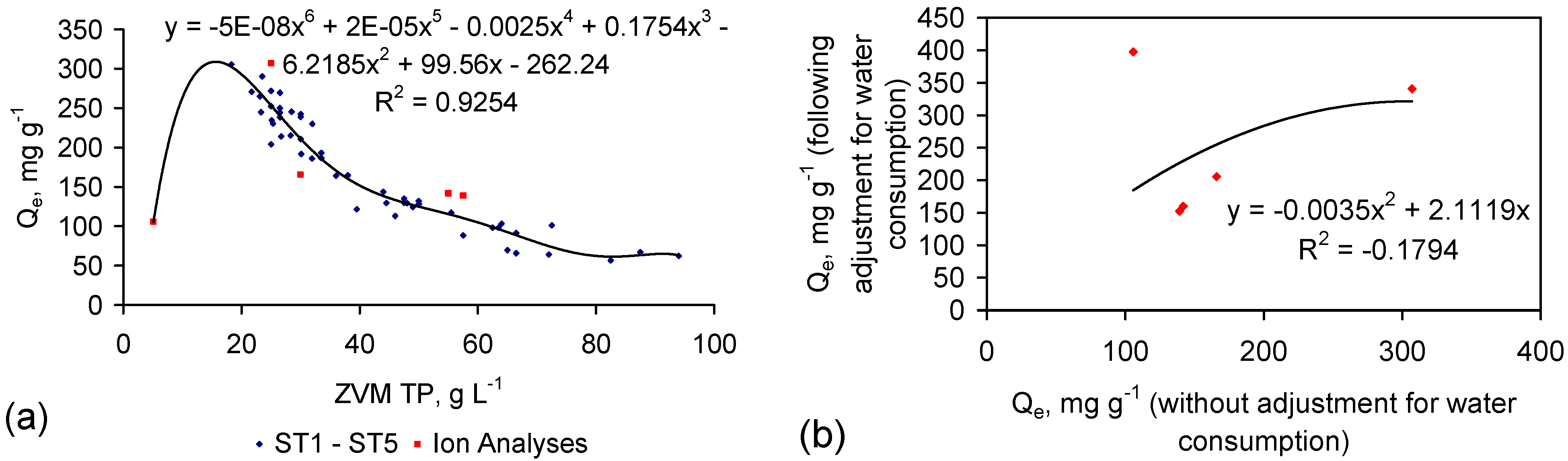
The analysis in Figure 8 does not consider water consumption during desalination. Integrating (into Figure 8) the salinity data in Table 1 (Table C1 and Table C2), demonstrates that Qe reaches a maxima at a ZVM TP concentration [Pw] of between 15 and 20 g·L−1 (Figure 9a).
The relationship between Qe calculated both before and after water loss consideration (Figure 9b) provides an estimate of:
This analysis demonstrates that the total amount of NaCl removed can approximate 10 g·L−1 for ZVM TP concentrations above 40 g·L−1 (Figure 9d).
Figure 9.
(a) Qe (without adjustment for water consumption) vs. ZVM TP concentration; (b) Measured relationship (Table 1) between Qe (without adjustment for water consumption) vs. Qe (with adjustment for water consumption); (c) Qe (with adjustment for water consumption) vs. ZVM TP concentration; (d) Total NaCl removed, g·L−1 vs. ZVM TP concentration; (e) Qe (with adjustment for water consumption) vs. Fe0 BET surface area, based on a ZVM TP concentration of 10 g·L−1 (for ST1-ST5, PS14) and 2.5 g·L−1 for PS7; (f) Total NaCl removed, g·L−1 vs. Fe0 surface area for a nominal ZVM TP concentration of 40 g·L−1. Ion analyses samples are: ST3b, ST3f, ST6d, PS4, PS5, PS7 (Table 1): Data: Appendix C. Surface Area Data: ST1–ST5 [6]; PS14 [6]; PS7 [28].

4.3.3. Impact of ZVM Particle Size
The [at+1] analysis established that NaCl removal is a function of as and Pw (Appendix F3). The measured relationship between Qe and as (Figure 9e,f), demonstrates that Qe increases with as.
This relationship confirms that it is possible for 1 g ZVM to remove >1 g NaCl [25]. This observation is consistent with a model of accretionary, polyionic, akaganeite/FeOOH nano rod formation where the bulk of the adsorbed NaCl is electrostatically bound in the hydration shells and the ionic layer surrounding each FeOOH, e.g., [22,23,25,78,79,90,91,92,93,94,95,96,97,98,99,100,108].
4.4. Desalination Associated with NaCl Concentration in the Pore Waters within the ZVM TP Bed
Molecular modeling demonstrates [96] that when the water contains 0.05–0.1 M NaCl·L−1, the Cl− concentrations associated with the ionic layer at the akaganeite crystal end (001) face are 7.34 M Cl−·L−1 [96]. The Cl− concentrations in the hydrated shell adjacent to the longitudinal (100), (110) crystal faces are 1.47 M Cl−·L−1 [96].
This situation can only arise if the Fe(H2O)63+ species create chemical gradients in the water which physically attract NaCl to the Fe(H2O)63+ species to enable akaganeite formation and growth [96].
The molecular modeling [96] for akaganeite formation creates an osmotic gradient between the hydrated shells surrounding the akaganeite and the surrounding water body [108]. Osmotic theory would expect the Cl− ions to migrate from the akaganeite water shell (and ionic layer) into the surrounding water body [108,109].
4.4.1. Osmotic Pressure
The osmotic pressure created between fresh water and the longitudinal water shell of the akaganeite nano-crystals is 3.6 MPa, where osmotic pressure [Op] is calculated as [Op] (MPa) = [c]RT [82,83], where [c] = salt concentration in the water (M·L−1), R = gas constant, T = temperature, K. At 25 °C, RT = 2.480 kJ·M−1 [108,109], and [Op] (MPa) = 2.480 [c].
Experiments which have examined the molar relationship between OH:Fe in water, in conjunction with the molar relationship between Cl:Fe in water, have established [110] that:
- No Cl− is observed in the first co-ordination shell of Fe in the polymers when OH:Fe > 2 [110].
These observations indicate that the critical control on the rate of desalination is the rate of discharge of Fen+ ions into the pores within the ZVM mass and the ability of those pores to access saline water from the overlying water body. This process creates an effective osmotic gradient between the water body and the pore water surrounding the ZVM, which results in a net migration of NaCl into the pore waters surrounding the ZVM.
This mechanism predicts that in a diffusion environment [the salinity of the hydration shells] > [the salinity of hydrated ZVM TP + associated pore waters] > [Salinity of the principal water body].
4.4.2. Role of Hydration Shells
The β-FeOOH polymorph is an unstable structure, which is stabilized by Cl− [111]. When Cl− is absent, or drops below a critical level in the pore waters within the ZVM TP, another FeOOH species (e.g., goethite) will form [111].
The Al0 in the ZVM TP corrodes in water to produce Al(–OH2)n+ sites and is able to remove both Na+ and Cl− ions as: [(AlOH20.5+)(Cl−)], [(Al3O0.5−)(Na+)], and [(Al3OH0.5+)(Cl−)] [112]. Both Fe and Al adopt similar and complementary surface sites [111,112,113].
The precipitated FeOOH species form a repeating sequence of atoms and radicals [113]:
- terminal surface (no hydration, e.g., FeOH0.5−): (OH)–(OH)–Fe–O–O–Fe–R (where R = a repeat of the stoichiometric atomic layer sequence, or tethering surface. R can included hydrated layers);
- interface terminal surface (no hydration, e.g., FeOH20.5+): (H2O)–(H2O)–(OH2)–(OH)–Fe–O–O–Fe–R
- double hydrated terminal surface: (H2O)–(H2O)–(OH)–(OH)–Fe–O–O–Fe–R
- double hydrated interface terminal surface: (H2O)–(H2O)–(OH2)–(OH)–Fe–O–O–Fe–R
The Na+ ions are removed within the (H2O)–(H2O)–(OH)–(OH)–Fe–O–O–Fe–R sequence. The Cl− ions are removed within the (H2O)–(H2O)–(OH2)–(OH)–Fe–O–O–Fe–R sequence.
The example illustrates two hydration shells. The actual number of hydration shells can exceed 2, i.e.,
(H2O)–……..–(H2O)–(OH)–(OH)–Fe–O–O–Fe–R and (H2O)–……–(H2O)–(OH2)–(OH)–Fe–O–O–Fe–R
The hydration shells can account for >41% of the weight of FeOOH [114], and increase the effective surface area of the FeOOH [114]. 5 hydration shells approximate to 46 wt % of FeOOH·mH2O.
This general phase structuring allows NaCl removal to be undertaken at the terminal sites and within the corrosion zone. It potentially allows any hydrated FeOOH species to be structured to form an effective desalination agent.
4.5. Role of Surface Charge and Capacitance in Assessing Desalination Efficiency
This section considers:
- the observed surface charge and capacitance associated with desalination;
- the capacitance characteristics of ZVM TP prior to use for desalination;
- the capacitance characteristics of the ZVM TP following desalination.
The trial results in Appendix C indicate that an understanding of surface charge and capacitance may allow elucidation of the ZVM TP characteristics required to maximize Qe and reduce the time required to achieve a specific level of Qe.
4.5.1. Observations Made during Desalination
The increase in Qe which is associated with a decrease in pH (Figure 8c,d) can be linked to surface charge and proton uptake associated with FeOOH, i.e.,
- the proton uptake increases with both increasing salinity and decreasing pH; (e.g., at 0.1 M (5.844 g·L−1) NaCl proton uptake ([H+]ads (μM NaCl)−1·m−2 = −0.7006pH + 4.3174; at 0.01 M (0.5844 g·L−1) NaCl proton uptake ([H+]ads (μM NaCl)−1·m−2 = −0.7006pH + 3.8174 [116]), M = moles NaCl·L−1; m−2 refers to the BET surface area;
- the surface charge (C·m−2) increases (at 0.1 M (5.844 g·L−1) NaCl) with decreasing pH (e.g., Surface charge, C·m−2 = −0.0009pH2 − 0.033pH + 0.2957 [116]).
Qe increases as a function of the magnitude of the proton uptake shift and surface charge shift (Figure 10a,b). The Qe increase is also a function of pH (Figure 10c–j). A statistical correlation is present between Qe and the change in surface charge (i.e., the difference between the surface charge at the maximum pH and the equilibrium pH) (Figure 10g).
Decreases in salinity removal with time (e.g., Figure C1, Figure C2, Figure C3, Figure C4, Figure C5, Figure C6, Figure C7, Figure C8, Figure C9, Figure C10, Figure C11, Figure C12, Figure C13, Figure C14, Figure C15, Figure C16 and Figure C17) can be interpreted as being related to a decrease in the surface charge and a decrease in the availability of H+ sites.
4.5.2. Impact of Changes in Surface Charge on Qe during Desalination
Qe is maximized under conditions where the change in surface charge and change in proton adsorption (associated with the change in redox environment between the maximum pH and equilibrium pH) is minimized (Figure 10e–g).
The surface charge is proportional to the capacitance [117]. The capacitance increases with BET surface area of the FeOOH [91], e.g., Inner Layer Capacitance, C, μF cm−2 = −1.629as + 208.955; as = −0.61939C +128.27; C = Surface Charge/(D1 – D2); D1 = potential at the 0 plane. D2 = potential at the beta plane [117]. Surface Charge = C(D1 − D2) [117].
The surface area was calculated for the case where (D1 − D2) = 1 (Figure 10k). This analysis demonstrates that the surface area increases as Qe increases (Figure 10k), and the effectve surface charge decreases as surface area increases (Figure 10a).
The formation of FeOOH species such as goethite and ledidocrocite (which have a lower capacity for Cl− adsorption) may result in different surface charge relationships and lower NaCl adsorption rates [116,118].
Figure 10.
ZVM TP: Surface charge and Qe during desalination. (a) Qe (without adjustment for water consumption) vs. surface charge; (b) Measured relationship Qe (without adjustment for water consumption) vs. proton adsorption; (c) Surface charge vs. proton adsorption; (d) Maximum and equilibrium Eh vs. proton adsorption; (e) Qe (without adjustment for water consumption) vs. change in surface charge; (f) Measured relationship Qe (without adjustment for water consumption) vs. change in proton adsorption; (g) Expected Qe (without adjustment for water consumption) vs. surface charge; (h) Equilibrium salinity vs. change in surface; (i) Change in salinity vs. change in surface charge; (j) Desalination cycle shown by water pH vs. surface charge; (k) Qe vs. calculated FeOOH surface area, when (D1 − D2) = 1. Data: ST1a–ST5j.

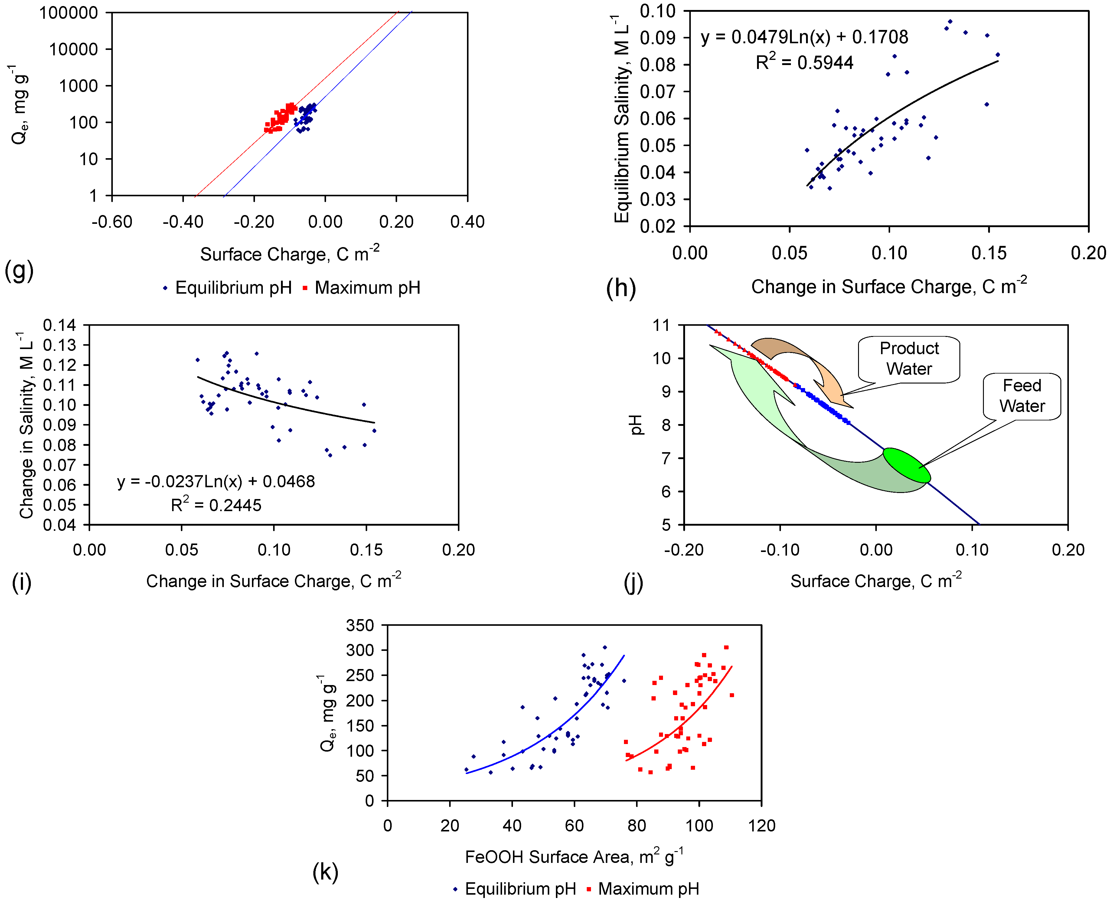
4.5.3. Measured Capacitance of the ZVM TP Prior to Usage for Desalination
Figure 10 demonstrates that Qe is a function of surface charge and capacitance. Two randomly selected Cu0 sheathed pellets (from the ZVM TP used in the analysis series ST1 to ST5 (which demonstrate desalination in Figure C5, Figure C6, Figure C7, Figure C8 and Figure C9)) were converted into dry cells by placing a steel electrode in the centre of the ZVM and a second steel electrode on the Cu0 shell of the pellet. The cell was placed on non conductive material (PVC) and attached to a multi-meter. The size of the current and voltage varied between pellets and with time.
These cells established that fresh ZVM TP pellets (manufactured by a Type B pre-treatment) placed in the saline water (Appendix C) were electrically active (Figure 11). The dry cells also established that the treated ZVM displayed significantly higher levels of electrical activity in the presence of NaCl + H2O (Figure 11).
Figure 11.
Measured currents and voltages as a function of time, associated with ZVM TP (ST1 to ST5 series) prior to usage for desalination. (a) Voltage vs. Time; (b) Current vs. Time. (c) Current vs. Voltage.
Figure 11.
Measured currents and voltages as a function of time, associated with ZVM TP (ST1 to ST5 series) prior to usage for desalination. (a) Voltage vs. Time; (b) Current vs. Time. (c) Current vs. Voltage.

4.5.4. Relationship between Capacitance and Desalination
The electrical analysis (Figure 11) demonstrates that ZVM TP can act as a charge receiver and storage unit (i.e., a capacitor or battery). In carbon steels (and carbon steel powders) the carbon content is typically within the range 0.15%–1.3% [119]. When the carbon content is <0.9% the corrosion sequence is Fe0 → FeII → FeIII [119]. When the carbon content is >0.9% the corrosion sequence is Fe0 → FeIII [119]. The FeIII species act as an anodic layer and carbon acts as a cathode.
The ZVM TP (formed from carbon steel) during desalination is effectively structured as a Fe0:Fe2O3:C capacitor, where the saline water acts as an electrolyte. Fe capacitor studies place FeIII species within their generic group (Fe2O3 [19]).
Under this model (e.g., [120]) NaCl removal at anodic sites (Fe2O3) will be associated with capacitor charging (e.g., formation of Fe3+ ion adduct species) while capacitor discharge will be associated with releases of NaCl into the water [120]. These gross changes are reflected in the EC measurements where a general EC decline is associated with oscillations between higher and lower EC values (Figure C1, Figure C2, Figure C3, Figure C4, Figure C5, Figure C6, Figure C7, Figure C8, Figure C9, Figure C10, Figure C11, Figure C12, Figure C13, Figure C14, Figure C15, Figure C16 and Figure C17).
4.5.5. Capacitance
The capacitance can be calculated [121,122] as:
where Cs = specific capacitance, F·g−1, i = average current (mA·s−1) applied, m = mass of ZVM, ΔE/Δt = average slope of the discharge curve after iR drop where i and R are current and resistance.
Cs = i/(m(ΔE/Δt)
The Energy Density, E, (Wh·kg−1) is [121]:
where (ΔV) (V) = the potential range. The power density, P (kW·kg−1) is [121]:
td = time (s) to discharge.
E = 0.5Cs (ΔV)2
P = E/td
The dry cells in Figure 11 analyze two situations:
- Cell 1 represents the typical capacitance associated with discharged ZVM TP prior to placement in saline water.
- Cell 2 demonstrates that in saline water (following, or during desalination), the presence of NaCl around the ZVM TP has the effect of charging the cell and increasing its specific capacitance. These features are quantified in Table 4.
Table 4.
Specific capacitance, energy density and power density associated with ZVM TP pellets prior to use in desalination. These pellets were used in ST1a to ST5j (Appendix C), Cell 1 and Cell 2. x = hours since start of measurement.
| Variable | Cell 1 | Cell 2 | |
|---|---|---|---|
| Current | mA | 0.08 exp(−0.24x) | 4.33 exp(−0.0119x) |
| R2 | 0.8463 | 0.408 | |
| Voltage | mV | 947.23 exp(−0.0216x) | 781.47 exp(−0.0028x) |
| R2 | 0.858 | 0.494 | |
| i | mA | 0.016 | 2.860 |
| m | g | 56.000 | 11.000 |
| (ΔE/Δt) | 0.01531 | 0.00081 | |
| Cs | F·g−1 | 0.018 | 321.208 |
| ΔV | V | 0.199 | 0.734 |
| E | Wh·kg−1 | 0.00036 | 86.411 |
| td | s | 12,469 | 4452 |
| P | kW·kg−1 | 0.00000003 | 0.01941 |
Table 4 demonstrates that the net impact of NaCl is to increase Cs, E and P. The energy density (E) of Cell 2 is comparable with the energy density recorded from Fe2O3:C composite capacitors (Figure 12).

4.5.6. Voltage/Current Changes Associated with the Cessation of Desalination
The gradual removal of Na+ and Cl− from the water will result in the gradual reduction in both the specific capacitance and the columbic efficiency with time. These factors when combined with the trapping of Na+ within the ZVM, will result in a major fading of the desalination rate after either a critical number of charge:discharge cycles (Eh:pH oscillations) has occurred [143], or the salinity (electrolyte concentration) drops below a specific level. This situation was demonstrated in all the trial examples when the desalination period was extended to Day 250 (Figure C1, Figure C2, Figure C3, Figure C4, Figure C5, Figure C6, Figure C7, Figure C8, Figure C9, Figure C10, Figure C11, Figure C12, Figure C13, Figure C14, Figure C15, Figure C16 and Figure C17).
The effective floor on desalination (or cessation of desalination) indicates that a minimum salinity (or electrolyte concentration) is required in order to drive the discharge reaction. Similar observations are associated with Na–Fe2O3:C battery analyses [143,144].
The current and voltage associated with discharge from the fresh pellets declined with time from a Level, L1 to a Level, L2 (Figure 13) In the presence of NaCl the initial current and voltage increased from a Level L1 to a Level L3 (Figure 13).
Figure 13.
Relationship between voltage and current associated with used ZVM TP pellets following desalination (ST1a to ST5j), L4, and the unused ZVM TP prior to desalination, Cell 1 (L1, L2) and Cell 2 (L3). The pellet series are labeled S1 to S5 to distinguish them from the analyses (ST1a to ST5j) in Appendix C, as the measurements were made 2 years after termination of the desalination trials.

The voltage and current produced by the pellets associated with ST1a to ST5j were measured two years after the conclusion of the desalination trials in order to investigate the impact of desalination on capacitance.
The measured current clustered at a Level L4 (Figure 13). The measured voltage was between L2 and L1. The ZVM pellets following conclusion of the desalination trials were in a discharged state where the discharged voltage is intermediate between L1 and L2. This demonstrates [143,144] that the effective cessation of desalination (Figure 13) is associated with a partially discharged capacitor. Appendix H addresses the significance of this observation for Na ion removal.
This interpretation (supported by electrical measurements) demonstrates that the initial model of NaCl removal by adsorption [20,21,25] is over-simplistic, and that focussing on the capacitance of the ZVM TP during manufacture will allow Qe to be increased and allow the time required to desalinate water to a specific salinity to be reduced.
4.5.7. ZVM TP Pellet Capacitance Following Desalination
The capacitance of each ZVM TP pellet used in trials ST1a to ST5j (Figure C5, Figure C6, Figure C7, Figure C8 and Figure C9) was measured following the cessation of desalination and the amount of charge stored in the pellets was calculated as:
Energy Stored, Es, (Joules) = 0.5[Measured Capacitance (F) × (Voltage (V))2] Potential Power Generated (W) = Es/Dissipation time, s
This analysis (Figure 14) establishes that the recovered (discharged) pellets have a stored charge in the range 0.00001 to 0.3 J. It was observed that if the pellets were subsequently moistened, the capacitance (F) increased by a factor of 100–1000. The dry pellets had a measured capacitance in the range 0.1–20 × 10−6 F. The pellets when in operation in a water body (at the conclusion of the desalination trials) had a capacitance (F) of between 10 and 20,000 × 10−6 F and had an effective stored charge within the range 0.00001 to 0.3 kJ (E = 0.0006 to 16.7 Wh·kg−1).
Figure 14.
Relationship between measured voltage and stored charge associated with ZVM pellets.

This observation is consistent with a desalination model where the capacitance comes from charge storage at the ZVM TP–electrolyte (water) interface [143] and the specific capacitance and current density reduces with time. This is discussed further in Appendix F2.2 and Appendix H and is illustrated in Figure F2, Figure F3 and Figure H1.
4.5.8. Desalination Model Associated with ZVM TP
In Fe0:Na–Fe2O3:C capacitors [143,144] structural dislocations resulting from Na+ release reduce the permeability (and efficiency) of the capacitor with time. The Fe2O3 section of the Fe0:Na–Fe2O3:C ZVM unit can be schematically viewed [89] as a composite slab (Figure 15) composed of different FenO2 layers (AB, CA, BC).
Figure 15.
(a) Schematic representation of the structural changes which occur in the anodic Fe2O3 schiller sheets (Figure F1) during desalination of water. Cs values are taken from Table 4 and Figure 15b; (b) Stored energy contained in the ZVM TP during desalination and following desalination.

The first stage in the desalination process is the formation of prismatic structures (e.g., colloidal nano-particles, or Schiller sheets) containing tetrahedral sites occupied by Fe3+. FeOOH grows as Schiller sheets, when templated on a substrate [87,88].
The initial Fe2O3 corrosion product adopts a cuboid structure (P3) dominated by prismatic sites of the form (AB, BC, AC) (Figure 15) during the initial part of the charge cycle [89]. The Na+ ions are accommodated at the octahedral sites located between the FenO2 layers (AB, CA, AB) [89]. This O3 structure develops during cell charging (desalination) [89]. The prismatic sites are energetically stabilized by the NaxO ions [89]. The glide vectors of the FenO2 layers during this transition can create a variety of staking faults in the crystal structures particularly during Na+ extraction (reversals of the desalination process) [89] caused by temperature, Eh and pH oscillations [5,6,18]. During Na+ extraction vacant face sharing tetrahedral sites are formed between the FenO2 layers (Figure 15) [89]. These sites are filled by Fe3+ (and other cations contained in the water) [89]. The Fe2O3–water interface is characterized by an outer layer of adsorbed H+ ions [145]. This positively charged surface attracts the negatively charged Cl− ions (which are present as Na+:Cl− dissolved ion adducts [145].
These observations demonstrate the type of Fe corrosion structure required in the ZVM TP to maximise NaCl removal.
4.6. Statistical Analysis of the Change in Salinity with Time
The analyses in C1 to C17 (collated in Figure 16) indicate that passive diabatic desalination at ambient temperatures is gradual with a progressive increase in the amount of NaCl removed with time. A proportion of trials showed an initial increase in EC due to the release of ions from the ZVM TP into the water. All of the trials established some level of desalination after 120–150 days. The highest levels of desalination were associated with the most saline water (i.e., the rate of desalination increases with increasing water salinity) (Figure 16).
Figure 16.
Statistical Trials: Relationship between EC change and the time interval which has lapsed following placement of the ZVM TP in the water. (a) Observed EC declines within 4 h; (b) ZVM TP concentrations associated with declines observed in a 4 h period; (c) Observed EC changes within 7 days; (d) Observed EC changes within 30 days; (e) Observed EC changes within 60 days; (f) Observed EC changes within 90 days; (g) Observed EC changes within 120 days; (h) Observed EC changes within 150 days; (i) Observed EC changes within 180 days; All the trials were undertaken simultaneously. Temperature: Figure 1.
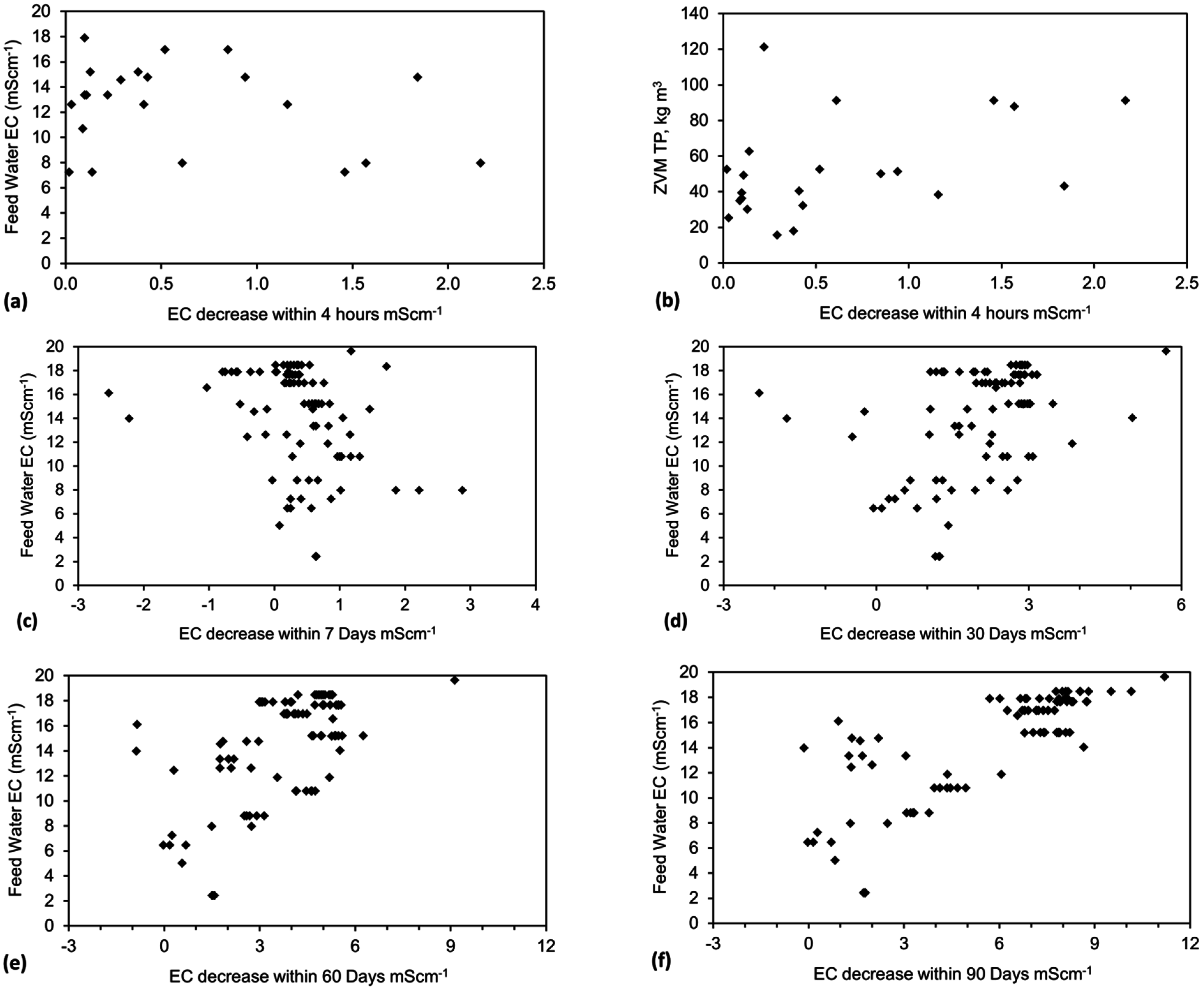

4.7. Cost of Desalination Using ZVM TP
Figure 16 and Figure C1, Figure C2, Figure C3 , Figure C4, Figure C5, Figure C6, Figure C7, Figure C8, Figure C9, Figure C10, Figure C11, Figure C12, Figure C13, Figure C14, Figure C15, Figure C16 and Figure C17 have established that placement of ZVM TP in water will result in a decline in water EC and salinity. The magnitude of the salinity decline is sufficient to have a substantial impact on crop yields (Figure B1) if the water is used for irrigation, or livestock yields if the water is used as livestock feed water (Figure B2).
4.7.1. Economics of ZVM TP without Reuse or Regeneration
The cost of Fe0 powders varies with time, grade, and location. The desalination cost is:
where Ws = water salinity drop required, kg·m−3; PFE = ZVM cost, $·t−1; Ru = number of times the ZVM TP is reused; Rv = Residual value, $·t−1, of the ZVM TP. The desalination cost reduces as Ws reduces, PFe reduces, Qe increases, Ru increases, Pw decreases, and Rv increases.
Desalination Cost, $·m−3 = (((Ws/Qe)(PFe))/Ru) − (PwRv)
For example, if the Fe0 powders are sourced for $400–$900 t−1, then based on Qe = 300 kg·t−1, 1 t Fe0 will be expected to remove 300 kg NaCl. The cost of desalination ($·m−3) is a function of the salinity reduction required (Figure 17) and the number of times a batch of ZVM TP can be reused.
Figure 17.
Desalination cost using ZVM TP, assuming no residual value for the ZVM TP and no reuse of the ZVM TP. Pw of 20 g·L−1, and Qe = 300 mg·g−1.
Figure 17.
Desalination cost using ZVM TP, assuming no residual value for the ZVM TP and no reuse of the ZVM TP. Pw of 20 g·L−1, and Qe = 300 mg·g−1.
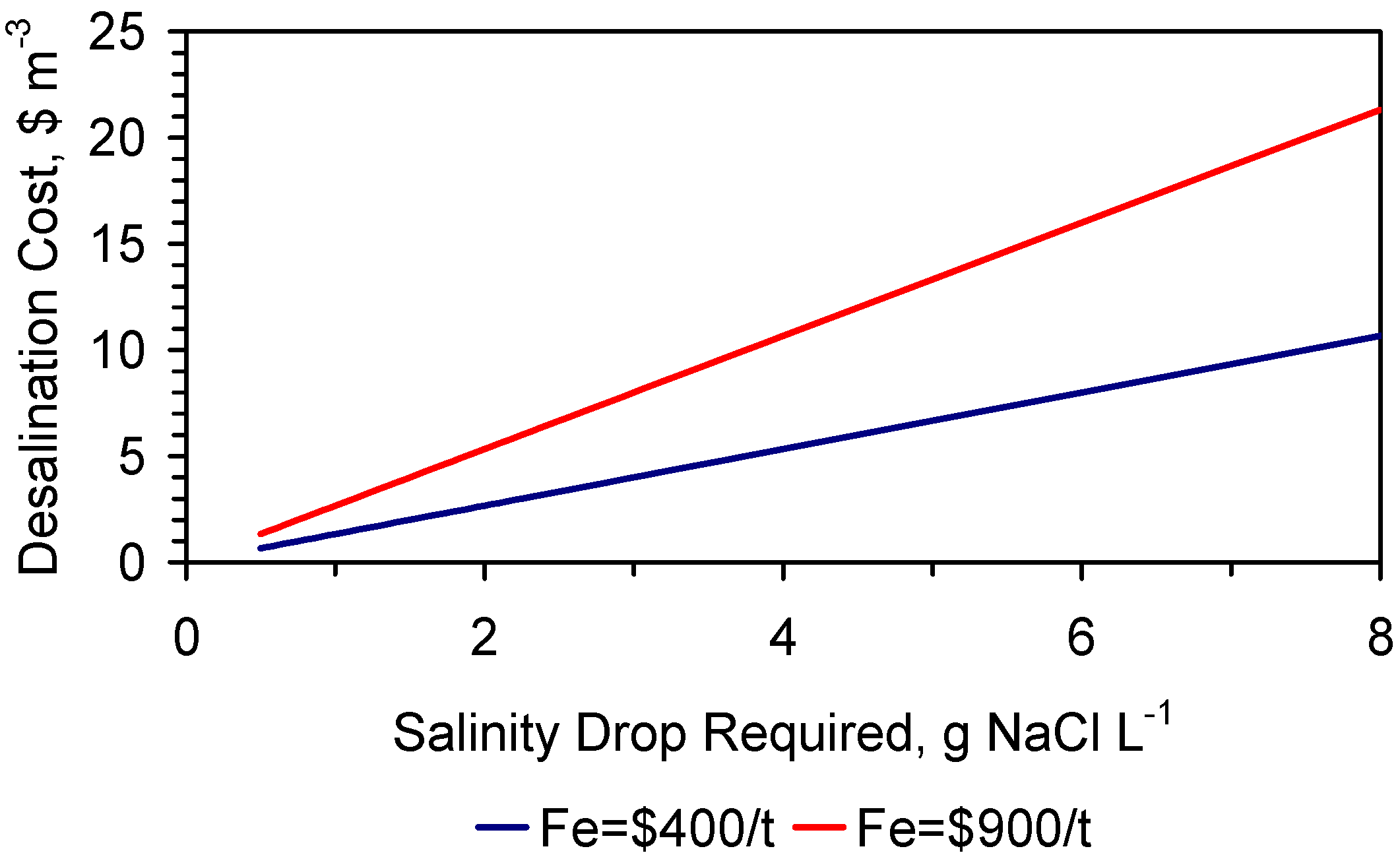
4.7.2. Reuse of the ZVM TP
The residual ZVM TP can be reused as a water treatment agent, or reprocessed for reuse as a desalination agent, or can be reused as an iron ore feedstock, or can be reused as a gas desulphurization agent (e.g., in an iron sponge), or reused in the construction of semi-conductors. The used ZVM TP can be regenerated as Fe0 (by reduction) or restructured (e.g., by NaCl removal) to allow reuse for desalination, or another purpose. An example life cycle for a batch of ZVM TP is illustrated in Figure 18.
Figure 18.
Example Life Cycle of a batch of ZVM TP which is used to desalinate water.

This residual value associated with reuse is location and application specific and will reduce the desalination cost further.
4.7.3 Reuse of ZVM TP as an Iron Sponge
The iron sponge gas desulphurization process has been in commercial use for >100 years [146]. It is based on the reaction [147,148]:
In gas: FexOy (s) + yH2S (g) = FexSy (s) + yH2O
In water: H2S (g) + H2O = H2S (aq) = HS− + H+
2Fe3+ (e.g., Fe2O3) + HS− = 2Fe2+ (e.g., Fe3O4) + H+ + S (s)
In water: H2S (g) + H2O = H2S (aq) = HS− + H+
2Fe3+ (e.g., Fe2O3) + HS− = 2Fe2+ (e.g., Fe3O4) + H+ + S (s)
1 t Fe (contained in ZVM TP) may remove 0.3 to 0.83 t S contained in a gas (or water) before regeneration. The sulphur is recovered by floatation from water [148]. Regeneration of the iron sponge by blowing air through the iron sulphide product [146,148], or by blowing air through water containing the 2Fe2+ (e.g., Fe3O4) [148]:
2Fe2S3 (s) + 3O2 (air) = 2Fe2O3 (s) + 6S + heat
2Fe3O4 (s) + 0.5O2 (air) = 3Fe2O3 (s)
2Fe3O4 (s) + 0.5O2 (air) = 3Fe2O3 (s)
Treatment of the nFe2O3 (s) + mS mixture with water under H2 or N2 at a pressure of 10.1 MPa (and elevated temperature) will result in the Fe2O3 catalysing the reaction [149]:
nS(s) + 2H2O = SO2 + (n − 1)H2S + (3 − n)H2
This cyclic process allows the ZVM TP to be reused for desulphurization, desalination and water treatment. A potential life cycle for a batch of ZVM is shown in Figure 18. The full life cycle allows the costs (depending on location and market conditions) associated with the ZVM and pre-treatment to be amortized over the various reuse/reapplication stages (Figure 18). Equation (21) demonstrates that any HS− ions in the water will be reformulated during desalination to release sulphur and H+ ions. This may allow both desulphuristion and desalination to be undertaken simultaneously.
The H2S removal operating costs for a sour gas producer using Fe based technologies vary with gas composition, competition between suppliers, field, and geographical location. An indicative operating cost is in the range $10,000–30,000 t−1 sulphur removed. This indicates that if the ZVM TP (following desalination) can be sold for reuse as a sulphur removal agent for $400–$950 t−1, the effective cost of desalinating the water will reduce to $0 m−3. The gross sales price is $550–$1,350 t−1 sulphur removed.
4.7.4. Reducing the Capital Costs Associated with Desalination
Qe and Pw define the amount of ZVM TP required to achieve a specific level of desalination. The time taken to achieve the required level of desalination is defined by the EC decline rate. The size of desalination facilities required is therefore a function of the amount of desalinated water required per unit time and the time taken to process a batch of water to a specific salinity level.
Trials ST1a to ST5j established that the salinity declined to a stable or equilibrium level and then abruptly ceased (Figure C5, Figure C6, Figure C7, Figure C8 and Figure C9). A number of freezing or partial freezing events occurred during the trials. The general decline in EC between the onset of the trial and the first freezing event was examined. In order to distinguish discussion of part of the trial, from the full trial data set, the following notation is used; (i) ST is replaced by S, i.e., ST1 becomes S1; (ii) The individual trial within a salinity grouping is labelled T1 to T10, i.e., ST1a becomes S1:T1. The individual plots of EC vs. time for each of these trials are provided as Figure D2, Figure D3, Figure D4, Figure D5 and Figure D6.
The decline in EC with time in each example can be modelled with a polynomial equation of the form:
where x = day number. In this study the first day of the trial is Day 59. A, B and C are constants. C represents the salinity (EC) at Day = 0. C can be replaced with salinity of the water at the onset of desalination. In this instance x can be replaced with the number of days since the onset of desalination. F = a factor required to the change units in the equation to mS·cm−1 (e.g., Figure E3) The observed polynomial regression equations for each trial are provided in Figure D2, Figure D3, Figure D4, Figure D5 and Figure D6.
EC, mS·cm−1 = (Ax2 − Bx + C)/F
The same data set (Figure D2, Figure D3, Figure D4, Figure D5 and Figure D6) could be interpreted using a regression power, or exponential function. The general exponential equation is:
where D = constant. The observed values of D ranged between 0.0042 and 0.0109 (Figure 19). R2 (for the exponential equation) was typically >0.91, but ranged between 0.604 and 0.995 (Figure D2, Figure D3, Figure D4, Figure D5 and Figure D6). Constant D reduces as the concentration of ZVM TP, or ZVM TP + Cu0 copper sheathing increases (Figure 19). The observed values of D and R2 are provided in Figure D2, Figure D3, Figure D4, Figure D5 and Figure D6 for Trials ST1a–ST5j).
EC, mS·cm−1 = (C·e(−Dx))/F
Figure 19.
Redox desalination constants (D) associated with an exponential regression correlation. (a) Constant D vs. ZVM concentration; (b) Constant D vs. weight of Cu0 pellet sheath; (c) Constant D vs. weight of ZVM + Cu0 pellet sheath; (d) EC vs. Length of desalination period (days), for the observed range of values of Constant D, and Constant C (initial salinity) = 17 mS·cm−1 at t = 0 days.

The unit cost of desalination ($·m−3) decreases as Pw decreases. The size of the facilities required to process a specific volume of water each year (and the length of time required to process a batch of water) decreases as Constant D increases.
Qe and Pw control the amount of NaCl that can be removed by a specific batch of ZVM and control operating costs. Constant D controls the size of the facilities required (capital costs), and associated land take required, to deliver a specific volume of water per unit time.
Trials PS15, and PS16 (see Section 6) demonstrate that Constant D can be increased to >0.04 by operating the desalination process in a pressured reactor (operated at <0.1 MPa) where air is replaced by CO2 and N2. For example, processing of 1000 m3 in an open tank or reservoir with Constant D = 0.07 (Figure 19) will take 148 days to reduce the salinity from 10 to 3.68 g·L−1. Operating the same ZVM TP (PS16) in a pressured reactor increases Constant D (Section 6) to 0.462. This will allow the same volume of water to be processed to the same salinity level (3.68 g·L−1) in 22 days. This would allow delivery of 1000 m3 of partially desalinated water over 148 days using a pressured batch reactor with a treatment capacity of 152 m3.
4.7.5. Improving the Economics of Partial Desalination by Increasing the Operating Temperature
The desalination can be defined in terms of a rate constant (kobserved) [18] which is linked to both the amount of ZVM and surface area of the ZVM in the water, where [Rad] = ([as]·[aa]). [Rad] represents the number of available reaction or adsorption sites on the ZVM TP. It follows that:
kobserved = kactual × [Pw] × [Rad]
At a constant [Pw] the reduction of NaCl to products must therefore adopt the general form [150]:
where m = the reaction order, k = rate constant. The [Rate] according to the Rate law relates the rate of reaction to the concentration of reactants (and catalyst) raised to various powers [150]. It therefore follows that if the concentration of NaCl in the water is changed from a concentration [C1] to a concentration [C2] the [Rate] of desalination must change to [150]:
Rate = k × [NaCl]m
Rate = ([C2]/[C1])m × k × [NaCl]m
The change in ([C2]/[C1])m accounts for all or part of the decline in the rate of desalination with time associated with different starting salinity concentrations.
The [Rate] can be calculated [90] as:
Rate = −Δ[NaCl]/Δt = ([C2]/[C1])m × k × [NaCl]m
The Arrhenius equation requires that [124]:
where A = frequency factor, E = activation energy, kJ·M−1, R = gas constant, T = temperature, K. It follows that the desalination rate will vary with temperature, and E, where different ZVM combinations will have different values of E.
k = Ae[−E/RT]
The desalination reaction will progress to equilibrium, where the equilibrium constant (Kc) is [18,150]
where ΔE0 = standard electropotential; n = number of electrons transferred; F = Faraday constant; ΔG0 = Standard Gibbs Free Energy. A change in state (e.g., T, Eh and pH) changes ΔG, ΔE and Kc.
Kc = [Products]a/[Reactants]b
ΔG0 = −RT·(lnKc)
ΔE0 = −RT/nF·(lnKc)
ΔG0 = −RT·(lnKc)
ΔE0 = −RT/nF·(lnKc)
4.7.6. Relationship between EC (Salinity) Reduction and Temperature
Equations (26)–(31) demonstrate that the desalination rate is a function of temperature. Therefore operation of a reactor at elevated temperatures may increase the rate of desalination.
A trial (CSD series (Table D1, Table D2 and Table 5)) was established using a reactor containing 8 L saline water and a 0.4 L cartridge containing ZVM TP constructed from 224 g Fe0 + 35 g Al0 (Table D1 and Table D2) The partial pressure in the water was maintained within the range 0–0.1 MPa. The same ZVM TP batch was reused in each of Trials CSD1a to CSD1d. The operating parameters were:
- Trial CSD1a: The trial duration was 15 h during which time the water temperature was raised from 5 to 50 °C. Air was bubbled through the water at a rate of 55 mL·min−1.
- Trial CSD1b: The trial duration was 124 h during which time the water temperature was raised from 5 to 44 °C. Air was bubbled through the water at a rate of 64 mL·min−1.
- Trial CSD1c: The trial duration was 30 h during which time the water temperature was raised from 7 to 39 °C. Air was bubbled through the water at a rate of 60 mL·min−1.
- Trial CSD1d: The trial duration was 11 h during which time the water temperature was raised from 7 to 36 °C. Air was bubbled through the water at a rate of 22 mL·min−1 for 4.7 h followed by 15 mL·min−1 80% N2 + 20% CO2.
The gases were not bubbled through the ZVM TP. The trial results are summarized in Table 5. This trial established that increasing temperature:
- increases the rate of desalination;
- allows the ZVM TP to be reused to sequentially partially desalinate batches of saline water;
- allows the salinity of the product water to reduce below 0.2 gNaCl·L−1.
| Trial | Feed Water | EC, mS·cm−1 | Salinity, g·L−1 | Product Water | EC, mS·cm−1 | Salinity, g·L−1 | NaCl Removed, g·L−1 | ||
|---|---|---|---|---|---|---|---|---|---|
| Eh, V | pH | Eh, V | pH | ||||||
| CSD1a | 0.277 | 6.150 | 4.540 | 2.500 | 0.167 | 6.500 | 0.544 | 0.194 | 2.306 |
| CSD1b | 0.188 | 5.920 | 4.540 | 2.500 | 0.130 | 6.900 | 0.556 | 0.200 | 2.300 |
| CSD1c | 0.088 | 6.700 | 4.760 | 2.625 | 0.219 | 6.020 | 1.830 | 0.888 | 1.737 |
| CSD1d | 0.174 | 5.970 | 5.450 | 3.000 | 0.233 | 5.440 | 3.670 | 1.882 | 1.118 |
The cost of reducing the average feed water salinity from 2.65 gNaCl·L−1 to an average salinity of 0.791 g·L−1 (CSD1a–CSD1d) (based on a Fe0 price of $400 t−1) is $2.8 m−3 ($2.28–$6.3 m−3 at a Fe0 price of $325–$900 t−1).
The product water from Examples CSD1a and CSD1b (Table 5) meet the EU, WHO and Indian definition of potable water. These results indicate that ZVM TP can be used to create potable water at temperatures of <50 °C over a period of <24 h. The cost of providing the potable water in CSD1a + CSD1b (based on a Fe0 price of $400 t−1) is $5.6 m−3 ($4.55–$12.6 m−3 at a Fe0 price of $325–$900 t−1).
Potable water definitions vary with country. Examples include:
Trials CSD1a and CSD1b established that a reduction in temperature from 50 to 44 °C increased the length of time required to produce potable water (<0.2 gNaCl·L−1) (feed water salinity = 2.5 g·L−1) from 15 to 124 h. Trial CSD1 demonstrates that operating ZVM TP (CSD1a) at a temperature in the range 50–75 °C will produce potable water within 15 h for a cost of <$2.8 m−3 from a small (e.g., <10 m3) or large scale (e.g., >10,000 m3) heated water tank.
Following completion of trial CSD1d, the residual water (0.4 L) in the manifold and ZVM cartridge was recovered (on recovery: Eh = 0.097 V; pH = 5.84; EC = 10.650 mS·cm−1; after 6 weeks storage: Eh = 0.166 V; pH = 7.41; EC = 17.12 mS·cm−1). These observations demonstrate the presence of a halocline between the main water body (EC = 3.67 mS·cm−1) and the manifold and ZVM container (EC = 10.650 mS·cm−1). They also demonstrate that:
- The ZVM TP modifies the salinity of the water adjacent to the ZVM TP by removing NaCl from the overlying water body.
- The removal of NaCl can occur when the water body is static (e.g., ST1a–ST5j series of trials) or when the bulk of the water body is in constant movement due to gas bubbling and the water column connecting the ZVM TP to the moving water body is static.
5. Results: ZVM TPA
The ZVM TP analyses established that the rate of desalination could be enhanced to allow partial desalination in less than 24 h if:
- The main water body was kept in a state of constant movement by an acid oxygenating (N2:CO2), or oxygenating (N2:O2) gas which was bubbled through the water;
- The ZVM TP was held in a container which was separated from the main water body by a static water column.
Earlier studies [21,25] had established that high rates of desalination occurred in a continuously stirred water column [21], or a water column which was subject to argon gas bubbling [25]. In both the earlier studies the ZVM was fluidised by the water movement in the reactor.
High rates of desalination were also observed when ZVM was mixed with ion exchange material (Ca-montmorillonite) [5] in a static water environment.
The ZVM TPA trials were designed to create a reaction environment where the main water body was kept in a state of constant movement by an acid oxygenating (N2:CO2), or oxygenating (N2:O2) gas which was bubbled through the water and the ZVM TPA was held in a container which was separated from the main water body by a static water column.
5.1. Desalination Using ZVI + Ion Exchange Material (ZVM TPA)
Experiments using mixtures of ZVM and Ca-montmorillonite (ion exchange material) [5,6] have established that the presence of the ion exchange material limits the maximum pH (attributable to ZVM) and creates a low variation between the maximum pH and the equilibrium pH. This can be reinforced by the addition of Al0 to the ZVM-ion exchange medium mixture [5]. The ZVM TP analysis has established that this will result in a low surface charge and a high Qe.
Layered aluminium silicates (e.g., feldspars, feldspar derivatives (clays), and zeolites) contain charged sites (when placed in water). These sites (and associated hydration layers) allow them to attract [Fe(H2O)6]3+ ions and act as nuclei for Fe species growth.
Switching from ZVM TP to ZVM TPA allows the [ZVI-ion exchange material] combination to be used to facilitate (and accelerate) NaCl removal at ambient temperatures.
5.2. Oxygenation and CO2
5.2.1. Oxygenated Water
In an oxygenated environment radicals which include NaO−, ClO− (Figure C37, Appendix H) develop:
Na+ + 0.5O2 + nH2O + 2e− = [(NaO)(H2O)n]•1−
Na+ + 0.5O22− + nH2O + e− = [(NaO)(H2O)n]•1−
Na+ + 0.5O2− + nH2O + 1.5e− = [(NaO)(H2O)n]•1−
Cl− + (1 + n)H2O = [(ClO)(H2O)n]•1− + 2H+ + e−
Cl− + Na+ + 0.5O2 + (1 + n + m)H2O = [(NaO)(H2O)n]•1− + [(ClO)(H2O)m]•1− + 2H+
Na+ + 0.5O22− + nH2O + e− = [(NaO)(H2O)n]•1−
Na+ + 0.5O2− + nH2O + 1.5e− = [(NaO)(H2O)n]•1−
Cl− + (1 + n)H2O = [(ClO)(H2O)n]•1− + 2H+ + e−
Cl− + Na+ + 0.5O2 + (1 + n + m)H2O = [(NaO)(H2O)n]•1− + [(ClO)(H2O)m]•1− + 2H+
5.2.2. Acid Oxygenated Water
In the presence of CO2 the radicals which include HCO3−, CO32−, NaO− and ClO− (Figure C37, Appendix H) develop:
Na+ + CO2 + (2 + n)H2O = [(CO3)(NaO)(H2O)n]•1− + 4H+ + 2e−
Na+ + CO2 + (2 + n)H2O = [(HCO3)(NaO)(H2O)n]•1− + 3H+ + 2e−
Cl− + CO2 + (2 + n)H2O = [(CO3)(ClO)(H2O)n]•1− + 4H+ + 4e−
Cl− + CO2 + (2 + n)H2O = [(HCO3)(ClO)(H2O)n]•1− + 3H+ + 4e−
Cl− + Na+ + 2CO2 + (4 + n + m)H2O = [(CO3)(NaO)(H2O)n]•1− + [(CO3)(ClO)(H2O)m]•1− + 8H+ + 6e−
Cl− + Na+ + 2CO2 + (4 + n + m)H2O = [(HCO3)(NaO)(H2O)n]•1−+ [(HCO3)(ClO)(H2O)m]•1−+6H+ + 6e−
5.2.3. Reaction Quotient Associated with Desalination in Oxygenated or Acid Oxygenated Water
5.2.4. Secondary Reaction Associated with Oxygenation by Air or Oxygen
Oxygenation of water creates the secondary reactions:
0.5O2 + H2O + 2e− = 2OH−
2OH− = H2O2 + 2e−
OH− + H+ = H2O
2OH− = H2O2 + 2e−
OH− + H+ = H2O
These result in a gradual increase in pH with oxidation to an equilibrium level (Figure C18, Figure C19, Figure C20, Figure C21, Figure C22, Figure C23, Figure C24, Figure C25, Figure C26, Figure C27, Figure C28, Figure C29, Figure C30, Figure C31, Figure C32, Figure C33, Figure C34, Figure C35 and Figure C36).
5.2.5. Adverse Impact of CO2 Demonstrated by ZVM TP
ZVM TP Trial CSD1c (Table 5) established that increasing the amount of H+ in the product water decreased the amount of desalination. This was confirmed by trial CSD1d (Table 5) where CO2 is used to supply a source of H+ [19]:
CO2 + H2O = HCO3− + H+
CO2 + H2O = CO32− + 2H+
CO2 + H2O = CO32− + 2H+
This adverse effect on desalination was not observed when the trials used ZVM TPA (Figure C33, Figure C34, Figure C35 and Figure C36).
5.3. Primary Desalination Mechanism Associated with ZVM TPA
Equation (32), Figure C37, and Appendix H demonstrate that the primary desalination mechanism involves oxidation of both Na+ and Cl− and the NaCl is removed as [(NaO)(H2O)]•1−, [(ClO)(H2O)]•1−, [(ClO–ClO)(H2O)]•, [(ClO-ClO)(H3O)]•1+ radicals. These radicals are removed by electrostatic attraction to the ZVI [68] and ion exchange material. This allows Qe > 1.0 [25]. It also allows a single charge of ZVM TPA to be reused multiple times at ambient temperatures.
This desalination mechanism was demonstrated using saline water (constructed using Cheshire halite (NaCl, rock salt)) and ZVM TPA, constructed from ZVM + K-feldspar (held in cartridges) using four series of trials. The four series of trials are: E143, E144, E145 and E146 (Table C5, Table C6, Table C7, Table C8, Table C9, Table C10, Table C11, Table C12 and Table C13, Table D3; Figure C18, Figure C19, Figure C20, Figure C21, Figure C22, Figure C23, Figure C24, Figure C25, Figure C26, Figure C27, Figure C28, Figure C29, Figure C30, Figure C31, Figure C32, Figure C33, Figure C34, Figure C35 and Figure C36).
Trials E143 and E144 were operated in a reactor containing 5.4 L water, with a basal ZVM TPA cartridge attached to the reactor via a manifold.
Trial E145 used a 114 L reactor containing 12 g·L−1 ZVM TPA. The test results from E145 indicated that a larger reactor (Trial E146) utilizing 240 L and a lower ZVM TPA concentration (1.67 g·L−1 ZVM TPA (Table C3)) would be more effective. The ZVM TPA in Trial E145 and E146 was held in a cartridge. In Trial E146, the ZVM TPA cartridge was separated from the main water column by a static water body.
5.4. Initial Trial: E143
The ZVM TPA charge (Pw = 25 gFe0·L−1) was reused 11 times in the E143 series of trials (Table C5, Table C6, Table C7 and Table C8, Table D3). Details of the trial feed water parameters, product water parameters, salinity change, water consumption, gas charge, gas composition, trial duration, temperature, and product water stability are provided in Table C5, Table C6, Table C7 and Table C8. The treatment:
- Achieved Qe(apparent) = 0.738 gNaCl·g−1 Fe0; Qe(after adjustment for water consumption) = 1.735 gNaCl·g−1 Fe0;
- Processed 2.4 L water·g−1 Fe0;
- Processed 59.4 L feed water (3.96 gNaCl·L−1 average salinity) to produce 48.28 L product water (2.28 gNaCl·L−1).
- Demonstrated a partial desalination cost of $0.9 m−3 feed water (for a Fe0 cost of $400 t−1).
Specific observations are:
- Product water pH > feed water pH when the CO2 content of the feed gas is 0%, otherwise Product water pH < feed water pH.
- NaCl removal decreased with increasing usage of the ZVM TPA.
- NaCl removal is associated with relatively high water consumption.
- The NaCl removal reaction is partially reversible. Some trials (Table C8) demonstrated increases in product water salinity when one, or more, of the water Eh, pH and/or temperature changed;
- The product water composition is stable and initial pH values in the range 5–6, are changed after 6 weeks to pH values in the range 6–7 and remained stable at that level thereafter.
5.4.1. Munsell Analysis
Following completion of the Trial E143k the manifold and ZVM TPA cartridge were drained separately and analyzed.
- 0.3 L (light orange colored; Munsell Parameters: hue = 5YR; chroma = 12; value = 7) water was recovered from the manifold (on recovery: Eh = 0.222 V; pH = 5.31; EC = 44.75 mS·cm−1; after 4 weeks storage: Eh = 0.275 V; pH = 6.47; EC = 50.17 mS·cm−1).
- 0.1 L (deep orange colored; Munsell Parameters: hue = 5YR; chroma = 8; value = 4) water was recovered from the cartridge (on recovery: Eh = 0.263 V; pH = 5.15; EC = 425.4 mS·cm−1 (3.92 M NaCl·L−1); after 4 weeks storage: Eh = 0.225 V; pH = 6.48; EC = 350.37 mS·cm−1).
These observations confirm that NaCl is concentrated in the static water beside the ZVI.
The Munsell parameters confirm that the nano-particles are akaganeite [155]. Akaganeite nano-particles darken in color as the particle size decreases [155], i.e., the Munsell value decreases [155]. The YR hue indicates that the n-Fe(OH) crystallites adopt a needle, or rod like, morphology [155]. A 5YR hue is consistent with the hydrated akaganeite (FeOOH) crystallites containing >0.15 M Na+·M−1 Fe0 [155].
5.4.2. Halocline Analysis
The average concentration of NaCl (g·L−1) in the cartridge approaches the eutectic concentration of NaCl at 23.3 wt % NaCl (37.6 wt % dehydrate (NaCl:2H2O)) [156] and may exceed the critical dehydrate concentration of 37.6 wt % [156]. The ZVM cartridge and manifold acted as a collector of NaCl. The high concentrations of NaCl indicate that direct NaCl precipitation can occur within the ZVM bed once the concentration of NaCl exceeds the eutectic concentration [156].
These observations demonstrate that the water body in the reactor can become structured during operation with separate haloclines forming between the main water body and the manifold, and the manifold/cartridge and the ZVM. Each of the three water zones identified has a separate density, with density increasing as salinity increases.
The major variable in each trial was the amount of, and type of dissolved gases (N2, O2, CO2), entered into the water. The permeability of the water (kw) to a migration location (within the water) away from the gas source decreases exponentially with increasing distance (Dw) [157]. The differences in oxygenation may also result in the development of a thermocline, where the temperature of the oxygenated layer is greater than the temperature of the anoxic layer [157]. Haloclines can be manufactured by placing less saline water on top of more saline water [158].
The observations in Table C4, Table C5, Table C6, Table C7 and Table C8 together with the development of chemoclines is consistent with a model that dimeric/ion adducts, or radicals, of the structure [(NaO)(H2O)n]•1−, [(Na)(H2O)n]•1+, [(Cl)(H2O)n]•1−, [(ClO)(H2O)n]•1−, [(ClO-OCl)(H2O)n]• are formed in the main water body and migrate (and are concentrated) by electrostatic attraction towards the ZVM TPA.
5.5. Long Duration Trial: E144
This trial sought to determine if increasing the treatment time using ZVM TPA (Pw = 9.4 gFe0·L−1), resulted in increased NaCl removal. The trial results (Table C9, Table C10, Table C11 and Table C12) established that:
- Product water salinity based on EC overestimated the actual water salinity (calculated from UV-visible spectrometry) due to the formation of nano-particles in the water;
- Desalination using ZVM TPA has an optimum treatment time within the range 1 to 24 h, though the amount of NaCl removed increases with time.
The trial demonstrated:
- ZVM TPA can be reused
- 32.4 L of feed water (3.02 gNaCl·L−1) produced 24.15 L of product water (1.56 gNaCl·L−1)
- An achieved Qe(apparent) of 0.932 gNaCl·g−1 Fe0; Qe(after adjustment for water consumption) = 1.25 gNaCl·g−1 Fe0;
- Processimg of 0.63 L water·g−1 Fe0;
5.6. Initial Upscaled Trial: E145
A trial (Figure C19) in a 114 L reactor containing 1.449 kg ZVM TPA held in 5 cartridges established an increase in pH to an equilibrium level, which was associated with a decrease in Eh. EC was found to increase to an equilibrium level. The UV-visible spectrometry established a salinity decline which was associated with nano particle formation (Figure C19).
This initial trial indicated (Figure C19) that the oxygenation level used would have been more effective in a larger water body containing less ZVM TPA.
5.7. Upscaled Trial: E146
Following completion of the trial E145, a cartridge containing 400 g ZVM TPA was removed from the reactor used in Trial E145. This cartridge was reused by being placed in a 240 L reactor (Pw = 0.52 gFe0·L−1). This trial series, termed Trial E146, (Table C13, Figure C20, Figure C21, Figure C22, Figure C23, Figure C24, Figure C25, Figure C26, Figure C27, Figure C28, Figure C29, Figure C30, Figure C31, Figure C32, Figure C33, Figure C34, Figure C35 and Figure C36) establishes that the cartridge can be used to treat 18 batches of water (average feed water salinity = 2.66 g·L−1; average product water salinity = 1.53 g·L−1). The desalination cost demonstrated was $0.011 m3 (for a Fe0 cost of $400 t−1). The 18th usage of the cartridge removed 3.6 g·L−1 (Table C13). The trial established that the reduced ZVM TPA concentration reduces the total nano-particle discharge into the water.
All the trials were undertaken using an air feed gas. Some of the trials were operated with a parallel trial using the same feed water (in a 5.4 L reactor), the Trial E144 ZVM TPA cartridge, and a feed gas containing 20% CO2 + 80% N2 (Figure C33, Figure C34, Figure C35 and Figure C36). These trials demonstrated lower rates of desalination than the air fed trials. The lower rates of desalination were associated with lower pH values and higher Eh values (Figure C33, Figure C34, Figure C35 and Figure C36).
In each example, using an air feed (Figure C20, Figure C21, Figure C22, Figure C23, Figure C24, Figure C25, Figure C26, Figure C27, Figure C28, Figure C29, Figure C30, Figure C31, Figure C32, Figure C33, Figure C34, Figure C35 and Figure C36), the product water pH is 1 to 1.5 units higher than the feed water, while the product water Eh is lower than the feed water Eh. The product water EC is higher than the feed water EC due to the formation of nano-particles. UV-visible spectrometry was used to assess the associated decline in salinity (Figure C20, Figure C21, Figure C22, Figure C23, Figure C24, Figure C25, Figure C26, Figure C27, Figure C28, Figure C29, Figure C30, Figure C31, Figure C32, Figure C33, Figure C34, Figure C35 and Figure C36).
A cross plot of feed water salinity vs. product water salinity (Figure 20), indicates that NaCl removal is a function of feed water salinity, where the total amount of NaCl removed increases with increasing feed water salinity. Removal rates are within the range 0.2–1 gNaCl·L−1·h−1.
Figure 20.
ZVM TPA example for the Trial Series E146a to E146q (Table C13). (a) Relationship between feed water salinity and product water salinity; (b) Relationship between feed water salinity and the rate of salinity removal.
Figure 20.
ZVM TPA example for the Trial Series E146a to E146q (Table C13). (a) Relationship between feed water salinity and product water salinity; (b) Relationship between feed water salinity and the rate of salinity removal.

Trials E145 and E146 confirmed the earlier observation [20] that placement of Fe0 powders in a circulating, oxygenated, water body will result in both an increase in EC and a decrease in salinity.
5.8. Cost of ZVM TPA Desalination
The economics of partial desalination using ZVM TPA is a function of both Pw and the number of times a specific charge can be reused. The number of times a specific charge can be reused will be a function of the feed water composition. Figure C19, Figure C20, Figure C21, Figure C22, Figure C23, Figure C24, Figure C25, Figure C26, Figure C27, Figure C28, Figure C29, Figure C30, Figure C31, Figure C32, Figure C33, Figure C34, Figure C35 and Figure C36 (Table C13) demonstrate that a single charge of 0.4 kg can be reused 18 times to partially desalinate >4.0 m3 (i.e., >10,500 m3·t−1 (ZVM + ion exchange material)). The ZVM TPA cost will vary with location, volume and commodity prices.
K-feldspar prices (free on board (FOB)) range from $45–$300 t−1 [159,160,161]. The iron powder prices range from $325–$900 t−1 FOB. The ZVM TPA (Trial E146) material costs fall within the range $132–$1020 t−1 FOB, i.e., the partial desalination cost range demonstrated by Trial E146 (Table C13) is between $0.009 and $0.026 m−3.
Trial E146 (Table C13) demonstrated that a single batch of 1 t ZVM TPA could be used (with reuse) to partially desalinate 10,500 m3 water. Additional costs include transport, loading/unloading, ZVM TPA disposal, water tanks, air compression and monitoring costs.
The ZVM TPA is designed for multiple reuse. The ZVM TP analyses established that a single use of a ZVM TP charge could result in high levels of desalination over a long time period. ZVM TPA Trials E144 and E145 (Figure 19, Figure 20 and Figure 21, Table C13) establish that a more appropriate application for ZVM TPA is as a multiple use desalination agent.
The decreases in salinity, e.g., 40%–55% (Figure 21), indicate that the ZVM TPA can be used to partially desalinate irrigation water, or livestock feed water, within a 24 h period.
Figure 21.
Partial desalination of water using ZVM TPA: E146, 0.4 kg ZVM TPA; 240 L water. (a) Regression relationship between feed water salinity and product water salinity; (b) Regression relationship between the proportion of the salinity removed and the feed water salinity; (c) Feed and product water salinities vs. number of times a batch of ZVM TPA is reused; (d) Amount of NaCl removed vs. number of times a batch of ZVM TPA is reused.

The minimum cost of partially desalinated water used for irrigation on the basis of an irrigation requirement of 1000 m3 water ha−1·a−1 is $12–$98 m3·ha−1·a−1. This compares with about $3000 m3·ha−1·a−1 if the desalinated water is produced by a large scale (>100,000 m3·d−1) desalination plant (reverse osmosis, or multi-stage flash distillation) at a sale price of $3 m−3 [36,37,38].
6. Cations and Anions (Pollutants) Removed during Desalination by ZVM TP and ZVM TPA
ZVM (Fe0, Cu0, Al0) (and ZVM TP, ZVM TPA) will remove a variety of pollutants and microbial organisms from water (Appendix A). Removal is achieved by either direct precipitation [18,19], or by incorporation into ZVM corrosion products [18], or by reduction of a pollutant to a lower oxidation state (e.g., many organic anions) [18], or by oxidation of a pollutant to a higher oxidation state [18]. A detailed discussion of the mechanisms involved in these processes is beyond the scope of this study, but is addressed elsewhere [18,19,162]. These pollutants are not removed by the ZVM, but are removed by the effect the ZVM has on the surrounding water. These effects are the increase in availability of: (i) e− to facilitate/catalyze electron shuttle reactions [18,19,162]; (ii) H+(ads) to increase the number of potential anion removal sites within the water; (iii) OH− to increase the number of potential cation removal sites within the water; (iv) adjustment of water Eh and pH to change the stable equilibrium form of a specific pollutant species.
Appendix A summarises the microbiota, cations and anions that can be removed by Eh and pH changes in the water which result from the presence of ZVM [18,19,162].
This study has demonstrated that ZVM TP and ZVM TPA create the same Eh and pH changes in water as ZVM [5,6]. Therefore it is reasonable to assume that similar pollutant removal mechanisms will apply to all three groups of material.
6.1. Cations and Anions (Pollutants) Removed during Desalination Using ZVM TP
Placement of ZVM TP in water results in the removal of a variety of cations and anions (Table C1, Table C2, Table C3 and Table C4). The proportion removed is a function of their original concentration, the composition of the water, treatment time, temperature and the ZVM TP composition.
The cations whose concentrations were reduced include: As, B, Ba, Ca, Co, Cu, Mg, Mn, Na, Ni, P, S, Si, Sr (Table C2, Table C3 and Table C4). The anions whose concentrations were reduced include: Cl, F, NO3, NO2, PO4, SO4 (Table C1). The concentrations of the cations and anions (apart from Na, Cl) in the water samples were low.
This ion removal data (Table C1, Table C2, Table C3 and Table C4) is cross plotted against NaCl removal in Figure C18. With the exception of sulphur (and sulphate) whose removal decreases with increasing NaCl removal, and manganese whose removal increases with increasing NaCl removal, there appears to be no direct correlation between cation/anion removal and NaCl removal. In all other cases, high levels of ion removal are associated with both low and high rates of NaCl removal.
The inter-relationship between desalination and the removal of other cations and anions in the water has not been specifically analysed in this study. The presence of high concentrations of other cations and anions (e.g., 1–400 g·L−1) may adversely impact on the rate of desalination.
6.2. Impact of Sulphates: ZVM TP and ZVM TPA
Sulphates can be present in chloride rich groundwater containing Fe, Na and other cations. In the presence of ZVI, sulphate interacts with the green rust product to preferentially displace Cl from the ion lattices (at low pH). The sulphate rich green rust product is termed Green Rust 2 (GR2) [163]. In the presence of sulphates the dominant FeOOH species is goethite [96,163]. The initial molar ratio, R, of SO42−/OH−, controls the formation of GR2 [163]. GR2 has only been observed when R > 0.5 [163]. In an environment containing both Cl− and SO42− ions, the overall reaction sequence is an initial precipitation of Fe(OH)2. This then transforms to GR1. The Cl− ions are then replaced by SO42− ions to form GR2 and can be subsequently oxidised to form lepidocrocite (γ-FeOOH) [164].
The boundary between GR1 and GR2 is defined by the relative concentration of Cl− and SO42− ions where EhGR2 = −0.507 + 0.4137 log [Cl−] − 0.2364 log [SO42−] [164]. The initial transition from GR1 to GR2 is made by the replacement of Cl− by SO32− [165]. This maintains the GR1 structure [165]. The SO32− ions are replaced by SO42− ions as the GR2 structure forms [165].
This results in the effective desalination rate decreasing as the effective sulphate removal rate increases. This situation is demonstrated by the ZVM TP analyses (Figure C18) and indicates that the desalination process may be more effective in either desulphurized water or sulphurous water where the initial molar ratio R < 0.5 [163] and Eh < EhGR2.
The transformation of GR2 to lepidocrocite is controlled by the relative concentration of SO42−, where Eh = 0.55 + 0.0148 log [SO42−] − 0.089 pH [166]. The relative position of this redox boundary is shown in Figure 22. The UV-visible spectral peaks [101] associated with each Green Rust (GR) species (GR1, GR2) are well defined (Table 3). These spectra allow the dominant entrained Fe corrosion species in the water to be identified (Table 3).
Figure 22.
Pourbaix diagram showing the Eh, pH regions where the dominant stable precipitate is Fe(OH)2, GR1, and GR2 in water containing both Cl− and SO42− ions.
Figure 22.
Pourbaix diagram showing the Eh, pH regions where the dominant stable precipitate is Fe(OH)2, GR1, and GR2 in water containing both Cl− and SO42− ions.

The FeOOH chemistry is complex. In the absence of Cl− ions, lepidocrocite forms [166]. In the absence of SO42− ions, akaganeite forms, e.g., [167]. Lepidocrocite is replaced by goethite as the SO42−:Cl− ratio increases at the transition from GR2 to FeOOH [167]. Akaganeite which forms at the GR1:FeOOH boundary is replaced by goethite as the SO42−:Cl− ratio increases [167].
The presence of high concentrations of SO42− ions will reverse any Cl− desalination (by incorporation) which is associated with GR1 or akaganeite. Na+ ions are incorporated with green rusts and the transformation from GR1 to GR2 is unlikely to expel the Na+ ions [168]. Both Na+ and SO42− ions are released as the GR2 transforms to goethite [168].
6.3. Impact of Sulphides: ZVM TP and ZVM TPA
In the presence of water, Fe2O3 (spp.) catalyse the transformation of HS− ions to elemental sulphur (Equation (21)). HS− is stable under reaction conditions [19] which have a significantly lower Eh than those observed in this study (Figure C1, Figure C2, Figure C3, Figure C4, Figure C5, Figure C6, Figure C7, Figure C8, Figure C9, Figure C10, Figure C11, Figure C12, Figure C13, Figure C14, Figure C15, Figure C16 and Figure C17). The lower Eh (without additional oxidation) is expected to adversely impact on the rate of formation of green rust and FeOOH species. HS− (without oxidation) can result in the formation of Fe1+xS, Fe1−xS, Fe3S4, Fe3+xS4, FeS2, The main iron sulphide precipitation zone is within the green rust/Fe(OH)2 precipitation zone, and can result in reassignment of some of the ZVM from desalination to sulphide removal (Figure 23).

6.4. Impact of Bicarbonates: ZVM TP and ZVM TPA
Bicarbonates (HCO3−) are a common constituent of most groundwater. In volcanic areas (such as those used to provide the base water in this study), the dissolved organic content is low (e.g., 1–18 mg·L−1) [171]. Natural bicarbonate concentrations in this water are in the range 10–150 mg·L−1.
6.4.1. Trial E146: ZVM TPA
The ZVM TPA Trials, E146, established that increasing the HCO3− content of the water (with associated acidification) either had (i) no effect on the rate of desalination, e.g., Figure C33; or (ii) reduced the amount of NaCl removed by 30%–50% (Figure C34, Figure C35 and Figure C36).
6.4.2. Trials PS15 and PS16: ZVM TP
Two ZVM TP trials (PS15, PS16) were undertaken, using a reactor containing 3.5 L water (Table C1, Table C2, Table C3 and Table C4). The reaction environment in Trial PS15 was saturated with [16.79% CH4 + 16.88% H2 + 11.97% CO + 8.33% CO2 + 46.03% N2 for 79 days]. The reaction environment in Trial PS16 was saturated with [16.79% CH4 + 16.88% H2 + 11.97% CO + 8.33% CO2 + 46.03% N2 for 29 days] followed by [80% N2 + 20% CO2 for 135 days] followed by [100% N2 for 46 days].
The associated Eh, pH, and EC for the feed and product waters establish a general rise in pH (Table 6), indicating that the dominant carbonate species is a mixture of HCO3− and CO32− [19]. Both examples PS15 and PS16 demonstrated a substantial removal of NaCl (Table 6, Table C1, Table C2, Table C3 and Table C4).
Trial PS15 removed 9.51 gCl−·L−1 + 1.29 gK+·L−1 + 6.23 gNa+·L−1 over 79 days. The normalized molar removal ratio was: 1 Cl−: 1.26 Na+:0.54 K+. The normalised removal ratio is calculated as (K or Na Removed/K or Na in Feed)/(Cl Removed/Cl in Feed). Trial PS 16 removed 23.07 gCl−·L−1 + 15.35 gNa+·L−1 over 121 days. The normalized molar removal ratio was: 1 Cl−:1 Na+.
Trial PS16 reused the ZVM TP used in Trial PS15 and increased the amount of ZVM TP present (Table 6). These trials demonstrated:
- ZVM TP can be reused if it is held in an oxygen free environment.
- In an oxygen free environment, ZVM TP can increase the desalination rate [Constant D] to a value in the range 0.0128–0.0462. This compares with a [Constant D] of 0.004–0.011 using ZVM TP from the same batch in an oxygenated environment.
- Desalination using ZVM TP can occur when the water contains bicarbonate or carbonate ions.
| Water | Feed and Recovered Product Waters | pH | EC, mS·cm−1 | Storage Period, Years | Product Water Following Storage | pH | EC, mS·cm−1 | HCO3−, g·L−1 |
|---|---|---|---|---|---|---|---|---|
| Eh, V | Eh, V | |||||||
| PS15 | ||||||||
| Feed | 0.207 | 6.14 | 57.49 | - | - | - | - | - |
| Product | 0.094 | 9.49 | 31.12 | 1.11 | 0.220 | 8.9 | 35.70 | >10 |
| PS16 | ||||||||
| Feed | 0.207 | 6.14 | 78.16 | - | - | - | - | - |
| Product | −0.111 | 10.26 | 1.09 | 0.58 | 0.109 | 9.18 | 1.25 | 1.14 |
6.4.3. Desalination in an Alkaline Bicarbonate Saturated Anoxic Environment: ZVM TP
In this anoxic environment the ZVM TP (PS15, PS16) will corrode to have a Fe3O4 interface between the Fe0 and the FeIIFeIII corrosion layers [172]. High rates of desalination occur (Table 6). The Fe0 corrodes directly to form a GR1 structure containing HCO3− [73,172]. In the presence of sulphate, the GR1 transforms to GR2 [172,173]. The redox boundary between GR1 (CO32−) and GR2 (SO42−) approximates to the redox boundary between GR1 (Cl−) and GR2 (SO42−) (Figure 18). When sulphate is absent, the dominant green rust is green rust carbonate containing some Cl− ions [173]. GR1 (Cl−) is absent, even when the Cl−:HCO3− ratio is >40 [73]. The presence of carbonate-bicarbonate increases the rate of cathodic and anodic reactions and accelerates the rate of corrosion [174]. High corrosion rates are maintained by the interaction of Fe2+ species with HCO3− and the reduction of protons supplied by HCO3− ions [174]. A rapid decrease in corrosion rates is observed when the pH is decreased to move the reaction environment away from the CO32−:HCO3− buffer zone [174]. When the water contains no Cl− ions the GR1 (CO32−) will oxidize to the FeOOH species, goethite [73].
6.4.4. Impact of CaCO3 or MgCO3 in the Water: ZVM TP and ZVM TPA
The presence of CaCO3 or MgCO3 in the water (i.e., a Ca2+ − HCO3−, or Mg2+ − HCO3− groundwater type) will result in the formation of GR1 (CO32−) [172]. Trials PS15 and PS16 demonstrate that ZVM is able to desalinate a mixed ground water type containing [HCO3− + Na+ + K+ + Cl−] or [HCO3− + Na+ + Cl−].
6.4.5. Impact of Chlorinated Organic Compounds in the Water: ZVM TP and ZVM TPA
TCE (trichloroethylene) removal experiments in water containing Ca2+ − HCO3−, or Mg2+ − HCO3−, or Na+ − Cl− have established that passivation of the ZVI surface by GR1 (CO32−) reduces the ability of ZVI to dechlorinate hydrocarbons [175]. This may indicate that the dechlorination process involves a GR1 (Cl−) intermediate. In water containing high concentrations of NaCl, hydrocarbon dechlorination rates are inhibited due to competition for available sites by Cl− ions [175].
6.4.6. Bicarbonate/Carbonate Buffers: ZVM TP and ZVM TPA
The carbonate environment contains an acidic (H2CO3:HCO3− or CO2:HCO3−) buffer, and an alkaline (HCO3−:CO32− or CO2:CO32−) buffer [19].
The pH in the proximity of the alkaline buffer is a function of the ratio of log (CO32−/HCO3−) or log (CO32−/pCO2)
Examples PS15 and PS16 (ZVM TP) were operated in the vicinity of the alkaline buffer, where: Observed pH = 10.34 + log (CO32−/HCO3−) [19], or in the presence of CO2, where: Observed pH = (18.14 + log (CO32−/pCO2))/2 [19].
The examples in Trials CSD1 and E146 (ZVM TP and ZVM TPA) were operated in the vicinity of the acidic buffer, where: Observed pH = 6.38 + log (HCO3−/H2CO3) [19], or in the presence of CO2, where: Observed pH = (7.81 + log (HCO3−/pCO2) [19].
The example MT1d (Figure C13) investigated the effect of acidified carbonate (formic acid + calcium carbonate) on desalination. This example demonstrated that first placing the water in the H2CO3 regime and then using CaCO3 to increase the pH to move the water across the H2CO3:HCO3− buffer and into the HCO3− buffer resulted in a progressive increase in pH. As the pH increased above 7 and the Eh increased to >0.1 V, the EC demonstrated a rapid drop of >5 mS·cm−1 as dissolved species, Fen+, Ca2+, Na+, Cl− were removed.
6.4.7. Acid Bicarbonate Buffer: ZVM TP and ZVM TPA
Example analyses at the acid bicarbonate buffer demonstrated (Trials CSD1d, E143, E144, E146) a very low HCO3−/pCO2 ratio which was accompanied by partial desalination of the water, e.g.,
Trial CSD1d demonstrated:
- Table 5: HCO3−/pCO2 ratio = 0.004266:1; HCO3−/H2CO3 ratio = 0.1022; Feed water = 3 g·L−1; Product water = 1.88 g·L−1. Desalination time required = 16 h;
Trial E143 demonstrated (Table C5, Table C6, Table C7 and Table C8):
- E143b: HCO3−/pCO2 ratio = 0.1023:1; HCO3−/H2CO3 ratio = 2.74; Feed water = 4.44 g·L−1; Product water = 1.67 g·L−1. Desalination time required = 16.5 h;
- E143c: HCO3−/pCO2 ratio = 0.0109:1; HCO3−/H2CO3 ratio = 0.299; Feed water = 4.81 g·L−1; Product water = 2.11 g·L−1. Desalination time required = 15 h;
- E143d: HCO3−/pCO2 ratio = 0.0135:1; HCO3−/H2CO3 ratio = 0.343; Feed water = 5.37 g·L−1; Product water = 2.99 g·L−1. Desalination time required = 15.5 h;
- E143e: HCO3−/pCO2 ratio = 0.0229:1; HCO3−/H2CO3 ratio = 0.594; Feed water = 6.48 g·L−1; Product water = 4.95 g·L−1. Desalination time required = 15.5 h;
Trial E146 demonstrated:
- 13th Reuse (Figure C33): HCO3−/pCO2 ratio = 0.00195:1; HCO3−/H2CO3 ratio = 0.063; Feed water = 1 g·L−1; Product water = 0.35 g·L−1. Desalination time required ≤ 3 h;
- 14th Reuse (Figure C34): HCO3−/pCO2 ratio = 0.00219:1; HCO3−/H2CO3 ratio = 0.072; Feed water = 1.1 g·L−1; Product water = 0.7 g·L−1. Desalination time required ≤ 4 h;
- 15th Reuse (Figure C35): HCO3−/pCO2 ratio = 0.00275:1; Feed water = 2.05 g·L−1; Product water = 1.6 g·L−1. Desalination time required ≤ 9 h;
- 16th Reuse (Figure C36): HCO3−/pCO2 ratio = 0.00245:1; Feed water = 5.83 g·L−1; Product water = 1.8 g·L−1. Desalination time required ≤ 17 h;
Trial E143i (Table C5, Table C6, Table C7 and Table C8) established that if the ZVM TP had previously been operated in an environment containing a high HCO3−/pCO2 ratio (0.524:1) which is then reduced to (0.0087:1), this change is associated with a discharge of previously removed NaCl into the product water.E144 established (Table C9, Table C10, Table C11 and Table C12) that desalination ocurred at the acid bicarbonate buffer.
In each example the amount of NaCl removed was in the range 0.2–5 g·L−1. The E146 control trials (Figure C33, Figure C34, Figure C35 and Figure C36) where the trial was operated using 80% N2 + 20% CO2, and repeated using air (78% N2 + 21% O2) demonstrated similar levels of desalination in each example. This indicates that the type of oxygenating gas does not markedly affect the rate of desalination over the pH range 5–8.
6.4.8. Alkali Bicarbonate Buffer: ZVM TP
Two trials (PS15, PS16) were operated at the alkali bicarbonate buffer (Table 6). Trial PS15 was operated with a (CO32−/pCO2) ratio of 6.92:1 and Trial PS16 was operated with a (CO32−/pCO2) ratio of 239.88:1. Trial PS16 demonstrates that high NaCl removal rates (Table 6) can be associated with a high (CO32−/pCO2). This example (Trial PS16) demonstrated a net reduction in salinity from 38.6 to 0.55 gNaCl·L−1 product water over 210 days (Table 1, Table C1 and Table C2) which was associated with a ZVM desalination cost in the range $67.6–$187.2 m−3 (based on a ZVM cost of $325–$900 t−1) + gas cost + reactor costs. Trial PS16 demonstrated a gross reduction in salinity (after consideration of water consumption during desalination) from 38.6 to 0.15 gNaCl·L−1 of feed water (Table 1). Trial PS16 demonstrates 8.07 gSO42−·L−1 removal (Table C1) and indicates that desalination of water with a high g SO42−·L−1 content is possible if the water has a (CO32−/pCO2) ratio of 239.88:1, or (CO32−/HCO3−) ratio of 0.88:1 (i.e., the reactor is operated to ensure that GR2 is not an intermediate reaction product).
6.5. Desalination of Water Containing Sulphates and Bicarbonates: ZVM TP and ZVM TPA
GR2 (SO42−) can template on an FeOOH corrosion surface [176]. Its formation requires [176] the presence of an excess of OH− ions in the water, where Fe(OH)2 sheets grow parallel to the FeOOH or Fe0 substrate, trapping anions within the accreting layer (e.g., Figure F1). The water composition can be defined in terms of a ratio R, where R = [OH−]/[Fen+], and in terms of the ratio of Fe3+/Fen+ ions (Figure 20) [176]. The initial accreting product (Fe(OH)2) will, under stable anoxic conditions, as the [Fe3+/Fen+] ratio increases start to accrete green rust (Figure F1) [176]. As the [Fe3+/Fen+] ratio continues to increase these green rusts will either form FeOOH species (Figure F1), or will be reduced (by adsorbed H+ and released H2 (g)) to form magnetite (Fe3O4) (e.g., Figure F1) [176]. Entrained precipitates formed under these conditions will be dominantly FeOOH sp. (e.g., Figure F1) [176]. This sequence of progressive oxidation is summarized in Figure 24.
The initial FeOOH species can be lepidocrocite which is transformed into goethite and then subsequently akaganeite. Goethite and lepidocrocite are the dominant species when Cl− ions are absent or a relatively high level of SO42− ions are present [176].
While the exact ratio of R required for each phase may be water composition dependent, the general reaction scheme remains the same (Figure 24), where the end points associated with green rust formation are either (Fe3O4) resulting from reduction, or FeOOH formed from continued oxidation [176]. The presence of the initial (Fe(OH)2), green rust intermediate and the FeOOH and (Fe3O4) end points is illustrated in Figure F1.
The trial results have demonstrated that desalination will progress if the water contains Cl−, or [Cl− + HCO3−, CO32−, CO2]. Sulphates will expel both Cl− and CO32− ions from the green rust structure and will change the final oxidized product to goethite or lepidocrocite. This change is associated with an inverse relationship where the rate of desalination decreases as the sulphate concentration of the water increases (Figure C18).
Figure 24.
Relationship between Ratio R, and Fe3+ content surrounding ZVI and the nature of the corrosion products growing in the waters and accreting onto the ZVI. Data: [176].
Figure 24.
Relationship between Ratio R, and Fe3+ content surrounding ZVI and the nature of the corrosion products growing in the waters and accreting onto the ZVI. Data: [176].
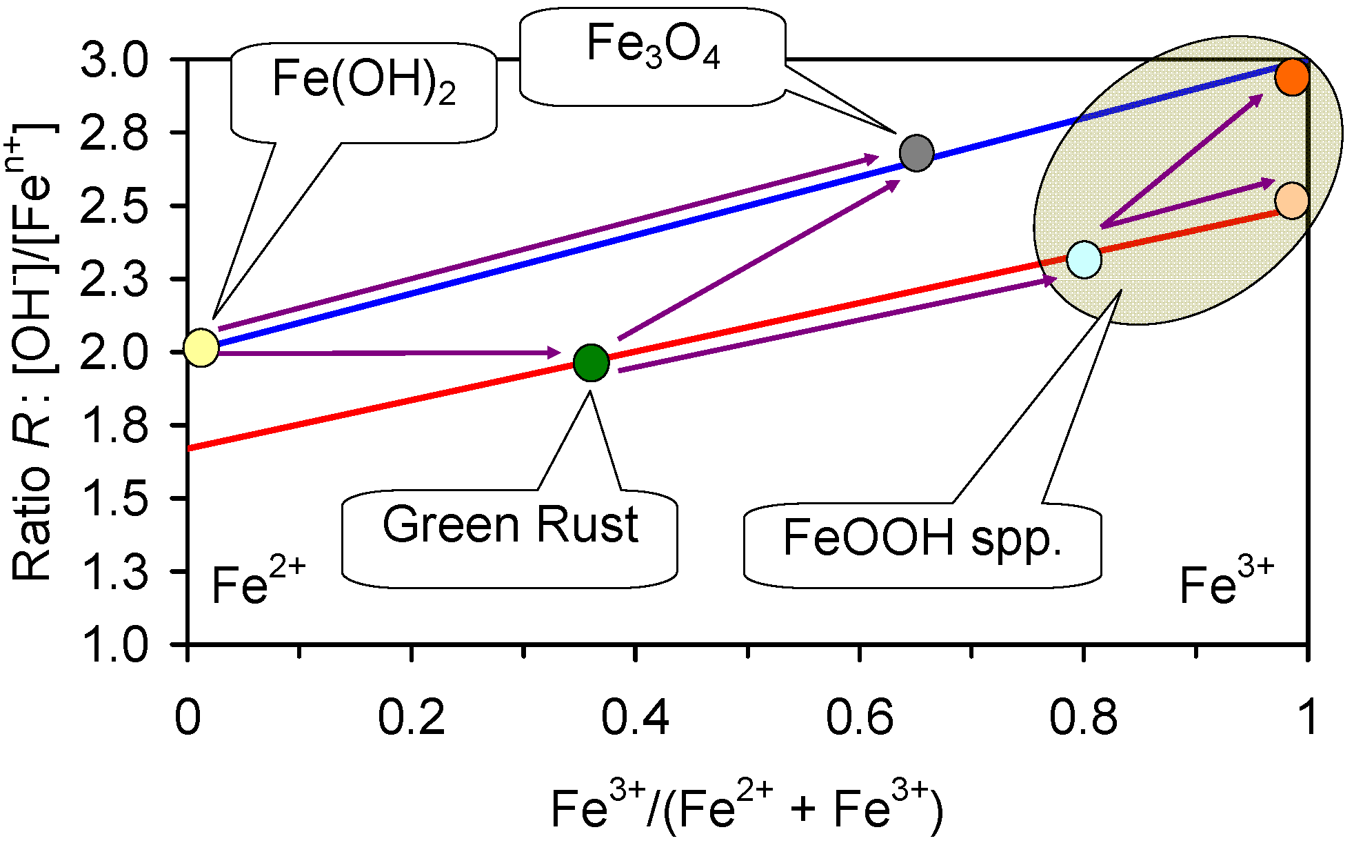
This water can be desalinated if an absorbent is used to first remove the sulphur. The residual salinated (desulphurized) water can then be desalinated using ZVM TP. Alternatively, Trial PS16 demonstrates that if the desalination process is operated in a pressured, reducing acid environment, both SO42− and NaCl removal will occur, provided the reactor is operated with a pH around the alkaline bicarbonate buffer.
7. Desalination Economics
The trials have demonstrated desalination costs. For example water with a salinity of:
- (1)
- 2.65 gNaCl·L−1 can be desalinated to:
- (a)
- ZVM TPA—multiple use:1.55 g·L−1 (over 1–24 h, Trial E146) and 6 gNaCl·L−1 reduced (Trial E146) to 3.35 gNaCl·L−1) for a cost of less than $0.009–$0.026 m−3. This cost is based on the demonstrated 18 times reuse of the same ZVM TPA charge. The number of times a ZVM TPA charge can be reused needs to be demonstrated in field operation, but may be in the range 20–100 times. This would allow the desalination cost to fall within the range $0.002–$0.024 m−3.
- (b)
- ZVM TP—multiple use:0.791 g·L−1 (over 11–124 h, Trials CSD1a–CSD1d) for a cost of $2.28–$6.3 m−3. This cost is further reduced if the used ZVM TP is sold for sulphur removal, or is reprocessed for reuse. The number of times a ZVM TP charge can be reused needs to be demonstrated in field operation, but may be in the range 5–20 times. This allows the desalination cost to fall within the range $0.4–$6.1 m−3. ZVM TP can be reused for sulphur removal from natural gas. This reuse application can result in a residual ZVM TP value which is greater than the cost of ZVM TP purchase and use as a desalination agent.
- (c)
- ZVM TP—single use: 0.2 g·L−1 (over <15 h, Trial CSD1) for a cost of $4.55–$12.6 m−3; Reuse of the ZVM TP for sulphur removal can reduce the cost of producing potable water to <$0.0 m−3, depending on the resale value realised for the used ZVM TP.
- (2)
- ZVM TP—single use: 11.05 gNaCl·L−1 can be desalinated to 3.34 g·L−1 (over 126 days, Trial ST3b) for a cost of $5.6–$22.48 m−3. Reuse of the ZVM TP for sulphur removal can potentially reduce the cost of producing partially desalinated water to <$0.0 m−3, depending on the resale value realised for the used ZVM TP.
- (3)
- ZVM TP—single use: 38.6 gNaCl·L−1 can be desalinated to 0.55 g·L−1 (over 210 days, Trial PS16) for a cost of $67.6–$187.2 m−3. Reuse of the ZVM TP for sulphur removal can potentially reduce the cost of producing partially desalinated water to <$3.0 m−3, depending on the resale value realised for the used ZVM TP.
These illustrative examples of costs demonstrated by the trials identify a number of potential market applications for the ZVM TP and ZVM TPA. They include:
- Partial desalination of irrigation water for arable crops;
- Partial desalination of livestock feed water;
- Partial desalination of water for municipal activities and grey water applications;
- Emergency water for people and livestock in areas affected by natural or anthropogenic disasters;
- Desalination of saline water in impoundments (including flowback water from shale gas wells and reject brine from RO desalination plants);
The economics of desalination is impacted by: (i) the number of times a specific batch of ZVM TP/ZVM TPA can be reused; and (ii) the residual (resale or reuse) value of the ZVM TP/ZVM TPA.
ZVM TPA can potentially be used for the rapid partial desalination of large volumes of water in most areas (for agriculture, municipal applications and greywater applications) and allows partially desalinated water to be delivered for a cost which is in the range $0.002–$0.026 m−3.
ZVM TP can fulfil a similar role for a similar or lower price in areas where there is high value added reuse market for the used ZVM TP as a gas desulphurization agent (e.g., onshore oil and gas fields in the USA). The ZVM TP can have a role as a single use agent, or a multiple use agent.
ZVM TP can fulfil a role as a single use agent to produce desalinated or partially desalinated water from a wide range of saline water (2–39 g·L−1). It is cost competitive with technology such as reverse osmosis (RO) in areas which are remote from infrastructure (e.g., disaster relief areas), or where the water is heavily fouled with other components, or where the water salinity is outside the applicable range for an RO plant.
7.1. Irrigation Market
UN Water estimates that globally, there are more than 16,000 desalination plants producing 70 million·m3·d−1 (25.5 Bm3·a−1) [177]. These plants consume 75.2 TWh (0.5% of global electricity consumption [177]). The basic cost of desalination (excluding extraction, pre-treatment, post desalination treatment, storage, distribution and wastewater disposal) is estimated for large scale (e.g., >100,000 m3·d−1) plants at $0.5–2.5 m3 for seawater desalination, and $0.2–2 m3 for brackish water desalination [178,179,180,181,182]. Small scale (<100 m3·d−1) desalination costs are estimated at $1 to more than 12 m3 [183].
An indication of the full cycle costs associated with large scale desalination is provided by the volume supply costs to industrial users in countries which rely on desalinated water for the bulk of their water supply (e.g., United Arab Emirates (UAE)). In the UAE, the tariff [184] for the supply of more than 20,001 imperial gallons (277.8 m3) month−1 is (April 2015) 4.6 fils/imperial gallon ($3.45 m3 (based on an exchange rate of 1 Dirham = US$0.27)). This indicates that actual cost of delivered water is in the range 3 to 7 times the basic desalination cost associated with the desalination plant. The supply cost of desalinated water to an agricultural holding may therefore fall within the range $3.5–$90 m3.
Desalinated water is currently used for agriculture in Spain (308,000 m3·d−1), Kuwait (130,000 m3·d−1), Italy (986 m3·d−1), and Bahrain (248 m3·d−1) [185]. Small quantities are also used in Qatar, and the USA [159]. Other countries such as Australia, Chile, and China are evaluating the feasibility of using water from desalination plants for agriculture [185].
In Australia, the sustainable potable groundwater resurce is about 10.2 Gm3·a−1, and the sustainable saline groundwater resource is about 15.5 Gm3·a−1 [185]. Current Australian agricultural water usage is 7.55 Gm3·a−1 [185]. This saline water resource is likely to be subeconomic for agricultural usage if the cost of extraction, desalination and delivery is >US$0.96 [185]. The desalination costs established by Trial E146, indicate that the cost of partially desalinating the sustainable saline groundwater resource of 15.5 Gm3·a−1 using ZVM TPA will be in the range $0.009–$0.026 m−3 ($140–$400 million·a−1 + extraction, tank, and distribution costs). This compares with the cost of water at the Melbourne desalination plant of $2.18 m−3 + distribution and storage costs [185].
It is estimated that four crops account for >40% of global agricultural water usage (rice = 21.3%; wheat = 12.4%; maize = 8.6%; soybeans = 4.6%) [181]. Other major consumers of irrigated water include cotton and grazing pasture [185]. Existing usage of desalinated water for agriculture has focussed on high value added crops which can sustain a relatively high water supply cost. High value crops include grape, fruit trees, nut trees, berry fruits, and vegetables (e.g., tomatoes, pepper, etc.) have lower irrigation requirements [185].
Ratios Used to Assess Irrigation Water Quality
Standard guidelines for water suitability for irrigation focus on a number of parameters including EC, TDS (total dissolved solids), SAR (Na+/((Ca2+ + Mg2+)/2)0.5), sodium percentage (100(Na + K))/(Ca + Mg + K + Na), Wilcox plot (sodium percentage vs. EC), Kelly’s ratio (Na/(Ca + Mg)), magnesium adsorption ratio ((100 Mg)/(Ca + Mg)), Doneen’s permeability index (100(Na + ((HCO3)0.5))/(Ca + Mg + Na)), chloroalkaline index [CAI-I = (Cl − (Na + K))/Cl; CAI-II = (Cl − (Na + K))/(SO42− + CO32− + NO3−), bicarbonate hazard index (mg·L−1 HCO3−/6100), residual sodium carbonate index ((CO32− + HCO3−) − (Ca2+ + Mg2+)) [27,186,187]. Water which has been partially desalinated by ZVM will show declines in sodium percentage and chlorine percentage. Other ions, Mg, Ca, bicarbonate/carbonate, sulphate, nitrate are also removed by the desalination process (Table C1, Table C2, Table C3 and Table C4), therefore analyses of product water suitability for irrigation based solely on ratio analysis of Na, K, Mg, Ca, Cl, HCO3/CO3, SO4, NO3 may not be meaningful. Desalination can remove Mg, Ca, Cl, HCO3 at the same rate, or a faster rate, than K, Na and Cl.
7.2. Cost of Irrigation Water
7.2.1. ZVM TP
The ZVM TP analyses (Table 1, Figure C1, Figure C2, Figure C3, Figure C4, Figure C5, Figure C6, Figure C7, Figure C8, Figure C9, Figure C10, Figure C11, Figure C12, Figure C13, Figure C14, Figure C15, Figure C16 and Figure C17) demonstrate a base desalination cost (based on a single usage at 20 kg·m−3) of $6.5–$18 m−3 (at a ZVM TP cost of $325–$900 t−1; desalination cost = Pw × Price/number of times the ZVM TP is reused). Trial CSD1 establishes that the ZVM TP can be reused at least four times without reprocessing or regeneration. This reduces the effective desalination cost to $1.6–$4.5 m−3.
Example ST3b (Table 1) demonstrates a reduction in salinity from 11.05 gNaCl·L−1 to 3.34 g·L−1 (over 126 days) for a cost of $5.6–$22.48 m−3. This change would increase the yields of barley, cotton, wheat, date palm, sugar beet, wheat grass, and Bermuda grass by between 300% and 800%, and would allow the agricultural holding to diversify to produce one or more of soybean, safflower, sorghum, rice, sesbania, flax, beans, figs, olives, cantaloupe, corn, lettuce, pepper and a wide variety of grasses for pasture (Appendix B, Figure B1).
Widespread usage of ZVM TP as an agricultural desalination agent requires the effective ZVM TP cost (following regeneration and reprocessing, or resale as a desulphurization agent (or for another application)) to reduce to <$58 t−1 or Pw to reduce to <4.5 g·L−1.
7.2.2. ZVM TPA
The ZVM TPA analyses (Trial E146) demonstrated a partial desalination cost of $0.009–$0.022 m−3. This was associated with a regression relationship (Figure 20) which links feed water salinity to product water salinity. This regression equation indicates that feed water with a salinity of 6 g·L−1, will produce a product water with a salinity of 3.35 g·L−1. This change in water salinity would allow a crop such as rice which cannot be grown in water with a salinity of >6 g·L−1 to be grown with a yield decrement of 40% [188] (Figure B1).
7.3. Potential Use of ZVM TPA to Boost Rice Yields
Rice yields and production costs vary with time, location and variety, but generally fall within the range: yield = 6–24 t·ha−1; wholesale price = $300–400 t−1; production cost = $300–$400 ha−1. Irrigation requirements for rice can fall within the range 5000–10,000 m3·ha−1·a−1 [189]. The cost of supplying partially desalinated irrigation water for rice paddy (based on Trial E146) is estimated to be $45–$220 ha−1·a−1 (i.e., a total rice production cost of $350–$420 ha−1). These costings indicate (Table 7) that the ZVM TPA partial desalination technology could be used to provide water for rice cultivation in areas which contain brackish saline water. Coupling partial desalination with high yield rice varieities may allow the expected rice yield to fall in the range 10–15 t·ha−1.
Field scale pilot trials are required to establish that the initial trials of ZVM TP and ZVM TPA technology can be upscaled to provide a low cost partial desalination approach for agricultural applications. The site specific water, including agricultural chemicals, fertilisers and microbiota, may interact with ZVM TP and ZVM TPA to accelerate, or retard, the desalination process.
Table 7.
Potential impact of partial desalination on the economics of rice cultivation. Assumptions: ZVM TPA (Trial E146); Desalination determination: Figure 20.
| Item | No Desalination | Partial Desalination | ||
|---|---|---|---|---|
| Irrigation, m3·ha−1 | 5000 | 10,000 | 5000 | 10,000 |
| Feed Water salinity, g·L−1 | 6 | 6 | 6 | 6 |
| Irrigation Water Salinity, g·L−1 | 6 | 6 | 3.35 | 3.35 |
| Rice Yield, t·ha−1 | - | - | - | - |
| Low | 6 | 6 | 6 | 6 |
| High | 24 | 24 | 24 | 24 |
| Yield Decrement | 100% | 100% | 40% | 40% |
| Actual rice yield, t·ha−1 | - | - | - | - |
| Low | 0 | 0 | 3.6 | 3.6 |
| High | 0 | 0 | 14.4 | 14.4 |
| Production Cost, $·ha−1 | - | - | - | - |
| Low | 300 | 300 | 345 | 390 |
| High | 400 | 400 | 500 | 620 |
| Rice price, $·t−1 | - | - | - | - |
| Low | 300 | 300 | 300 | 300 |
| High | 400 | 400 | 400 | 400 |
| Net Sales Revenue, $·ha−1 | - | - | - | - |
| Low | −400 | −400 | 580 | 460 |
| High | −300 | −300 | 5415 | 5370 |
7.4. Economic Implications of Corrosion Scale
ZVI desalination has been associated with a high surface area [20,21,25,190], indicating that the contact area between the Fe0 and water surface is important [15,18,191,192]. Experiments using Fe + organic chemicals have demonstrated [5,6,193,194,195,196,197,198,199,200] that increases in water salinity are associated with in an increase in the rate of degradation of the organic chemicals and (COx, HxCyOz). This is associated with the construction of simple organic compounds (CxHyOz, alkanes and alkenes), where carbon can act as both an intermediary and reactant and Fe acts as a catalyst [5,6,193,194,195,196,197,198,199,200]. Trials PS15 and PS16 demonstrate that the presence of CO, CO2 and CH4 can be associated with increases in the rate of desalination.
This study has demonstrated that the ZVM TP is electrically active and contains both cathodic and anodic centres. Under these circumstances the potential cathodic half reactions [150] in saline water are:
Na+ (aq) + e− = Na ΔE0 = −2.71 V
2H2O (l) + 2e− = H2 (g) + 2OH− ΔE0 = −0.83 V
Half reaction (Equation (38)) is favoured over half reaction (Equation (37)) [150]. This is confirmed by Figure D1 which demonstrates production of H2 (g) + 2OH− during desalination. Half reaction (Equation (38)) can result in a film of NaOH coating [201] the ZVI and a corrosion scale (Fe(OH)2, GR1, FeOOH) coating the ZVI [18,68,69,70,71,72,73,74,75,76,77,87,88,93,94,96,110,111,112,167,172,173,176,191,202,203,204].
Na+ + OH− = NaCl
Fe0 + nOH− = Fe(OH)n
Fe(OH)2 = Fe(OOH) + H+ + e−
Fe(OH)2 = Fe(OOH) + H+ + e−
The associated anodic half reactions are [124]:
2Cl− (aq) = Cl2 (g) + 2e− ΔE0 = −1.36 V
2H2O (l) = O2 (g) + 4H++ 4e− ΔE0 = −1.23 V
H2O is oxidised in preference [150] to Cl− at the anodic sites. However, as Cl− concentrations increase, overcharging (development of FeOOH [18]) at the anodic sites (corrosion scale) results in a switch from half reaction Equation (42) to half reaction Equation (41) [150]. Any Cl2 formed is removed, as demonstrated in Figure C37, by an anodic reaction as ClO−, e.g.,
Cl2 (aq) + 2OH− = 2ClO− + 2H+ + 2e−
This model [150] results (as demonstrated in Section 4) in the amount of NaCl removed (and corrosion scale formed on the ZVI particles) being directly proportional to the inherent charge generated by ZVM TP/ZVM TPA, via the Nernst relationships [150], where [150]:
Charge, coulombs = current (amperes) × time (seconds)
The charge associated with desalination is [150]:
Charge = (1/Molecular weight (MW) Cl−) × Faraday Constant (F) × Weight (W) of Cl− Removed
For reactions involving other species associated with corrosion (e.g., formation of Fe(OH)2, GR1, FeOOH) the charge is a function of e− [150]:
Charge = (1/MW(species)) × F/en × W (species) × en/Moles Species Weight of
Species formed or removed = (1/MW(species) × F/en × en/Moles Species)/Charge
en = Moles e− associated with removal of 1 mole of the contaminant species
Species formed or removed = (1/MW(species) × F/en × en/Moles Species)/Charge
en = Moles e− associated with removal of 1 mole of the contaminant species
These relationships demonstrate that the rate of corrosion (and GR1, GR2, FeOOH scale formation around the n-Fe0 particles) will increase with increased contaminant concentration (e.g., NaCl) and with increased oxidation of the water. This has been demonstrated experimentally [205,206] and is used in this study (ZVM TPA, Section 5) to combine accelerated iron corrosion by oxidation with accelerated desalination. The charge associated with the development of the corrosion scale can be linked directly to the effective pseudo-specific capacitance (pSC) associated with the corrosion reactions as [207]:
pSC, F·g−1 = charge/(Pw(Eht=0 − Eht=n))
7.5. Applicability to Specific Sites
This study has evaluated desalination in batch treatment sizes ranging from 0.2 L to 240 L. Commercial applications will require larger plant sizes and may require the consideration of more complex water chemistries. Scale up performance into the 10–1000 m3 reactor/tank size range and application of the process using complex saline water (e.g., seawater, flowback water) has not been trialled at this time. The desalination rates at a larger scale and with more complex feed waters may be higher than, or lower than, the rates recorded in this study. This study has not optimized the rate of desalination, but has demonstrated a number of different routes which can be trialled to optimise the desalination rate. Facilities, offsites, and land requirements associated with commercializing this technology will be location, size and application specific [208,209].
8. Conclusions
This study has demonstrated that partial desalination of water (combined with water treatment (cation and anion removal)) using pellets, particles and cartridges, has the potential to be a green, sustainable, economically viable commercial treatment option for some saline water bodies. The operating limits evaluated in saline water include:
- pH range = 2–12,
- Electrical conductivity range of the feed water = 2–78 mS·cm−1,
- Salinity range of the feed water = 1–39 gNaCl·L−1,
- Carbonate range in the feed water = 10 mg·L−1 to >10 g·L−1; sulphate ≤ 10.2 mg·L−1.
- Temperature range considered = −8 to 50 °C.
This treatment option can either be operated using:
- No external energy, or
- Pressurized (<0.1 MPa) air, or
- Pressurized (<0.1 MPa) acidic gas (CO2), or
- Pressurized (<0.1 MPa) anoxic gas (N2), or
- Pressurized (<0.1 MPa) anoxic, acidic, reducing gas (H2 + CO + CO2 + CH4 + N2).
The desalination rates observed:
- Increase with increasing temperature;
- Increase with decreasing particle size (and increased particle BET surface area);
- Are optimised using Pw = 0.3–20 gFe0·L−1;
- Are optimised by maintaining the ZVM TP/TPA in a static water body, while allowing the overlying water body to be circulating and pressurised using a reducing gas, or an oxidising gas.
The cost of reducing water salinity was demonstrated to fall in the range $0.002–$190 m−3.
The technology has applications for the desalination of irrigation water (example cost: $0.002–$0.026 m−3), desalination of livestock feed water (example cost: $0.002–$0.026 m−3) and the provision of emergency water in areas following the destruction of infrastructure (example cost: $4–$190 m−3).
Acknowledgments
This study was funded by DCA Consultants Ltd.
Conflicts of Interest
The author declares no conflict of interest.
Appendix A. Microbiota, Cations and Anions that Can Be Removed by ZVM
ZVM studies have established [18,19,162] that placement of ZVM in water can remove:
- (1)
- cations (M) present as: ions (Mn+), hydroxides [M(OH)xn+/−], peroxides [M(OOH)n+/−], oxides [MyOxn+/−], and hydrides [MyHxn+/−], M is one or more of: Ac, Ag, Al, Am, As. Au, B, Ba, Be, Bi, Ca, Cd, Ce, Cm, Co, Cr, Cs, Cu, Dy, Er, Eu, Fe, Ga, Gd, Ge, Hf, Hg, Ho, In, Ir, K, La, Lu, Mg, Mn, Mo, Na, Nb, Nd, Ni, Np, Os, P, Pa, Po, Pr, Pt, Pu, Re, Rh, Ru, S, Sb, Sc, Se, Si, Sm, Sn, Sr, Tb, Tc, Te, Th, Ti, Tl, Tm, U, V, Y, Yb, Zn, Zr, and nitrogen based cations, e.g., NH4+. These ions are removed by precipitation, or by transfer into another ionic species.
- (2)
- anions (A) present as:
- (a)
- ions held in a a monoatomic or polyatomic form: H, F, Cl, Br, I, At, O, S, Se, Te, N, P, As, Sb, C, Si, Ge, B;
- (b)
- oxides, e.g., arsenates (AsO43−), acetates (C2H3O2−), bicarbonates (HCO3−), carbonates (CO32−), chlorites (ClO2−), chlorates (ClO3−), chromates (CrO42−), hypochlorites (ClO−), dichromates (Cr2O72−), hydrogen phosphates (HPO42−), nitrates (NO3−), nitrites (NO2−), N2O22−, perchlorates (ClO4−), permanganates (MnO4−), oxalates (C2O42−), phosphates (PO43−), sulphates (SO42−), sulphites (SO32−), thiosulphates (S2O32−), S2O62−, S2O82−, S4O62−, HS2O4−, or [Mz][On]y−;
- (c)
- nitrogen based anions, e.g., thiocyanates (CNS−), cyanides (CN−);
- (d)
- These ions are removed by precipitation, or by transfer into another ionic species.
- (3)
- Dissolved organic species:, e.g., chloromethane (CM), trichloromethane (TCM), dichloromethane (DCM), tetrachloromethane, perchloroethylene (PCE), trichloroethylene (TCE), dichloroethylene (DCE), vinyl chloride (VC), hexachloroethane, tetrachloroethane, trichloroethane, dichloroethane, chloropropane (and related species), chlorobutane (and related species), chlorobenzene, (and related species), ethylene dibromide (EDB), perchlorate, polychlorinated biphenyls (PCB’s), azo dyes, atrazine, cyclonite/hexogen (RDX), dinitrotoluene (DNT), nitrosodimethylamine (NDMA), nitrocellulose, tetramethylenetetranitramine (HMX), trinitrotoluene (TNT), disinfection by-products (DBP’s), fertilizers, pesticides, herbicides, fungicides, methyl tert-butyl ether (MTBE), aromatics, hydrocarbons, hormonal pollutants. These species are removed by reduction and fragmentation to one or more compounds or ions.
ZVM is known to destroy or deactivate a variety of microbial organisms [18,162] including:
- (1)
- Alcaligenes eutrophus, Aspergillus versicolor, Bacillus cereuis, Bacillus subtilis var. niger, colliforms (e.g., Enterococcus faecium, Enterococcus faecilis), Cryptosporidium spp., Dehalococcoides spp., Daphnia magna, Dunaliella tertiolecta, Escherichia coli, Giardia spp., Hartmannella veriformis, Isochrysis galbbana, Klebsiella pneumoniae, Naeglaeria spp., Naeglaeria fowleri, Pseudokirchneriella subcapitata, Pseudomonas spp., Pseudomonas fluorescens, Pseudomonas aeruginosa, Salmonella typhimurium, Salmonella enterica, Salmonella paratyphi, Salmonella spp., Shigella spp., Staphylococcus aureus, Streptococci spp., Tetrahymena pyriformis, Thalassiorsria pseudonana, Vibrio parahaemolyticus, Vibrio cholerae,
- (2)
- Aichi virus, adenovirus 41, MS-2, Hepatitis A, norovirus, phiX174/FX174, rotavirus, T1, f2 virus, fecal coliforms, fecal streptococci, fungi, prions, viruses, protozoa, bacteria, algae.
Appendix B. Agricultural Significance of Partial Desalination
The income associated with most agricultural units fluctuates annually as a function of climatic variations and commodity prices. These economic changes make it difficult to justify the capital investment required (or to obtain financing) to install a reverse osmosis desalination unit or multi-stage flash distillation unit. These desalination facilities are designed to produce a constant rate of high quality desalinated water.
Most agricultural sites do have access to water storage facilities and their water usage varies both within a year and between years. Furthermore, the relatively low value of the agricultural crop on individual holdings requires a low unit water cost for desalinated water.
The saline water used in agriculture can be derived from riparian sources or groundwater. Its salinity can vary with time. Water disposal to groundwater from agricultural units (e.g., from irrigation) can result in an increase in salinity of the aquifer as leached salts infiltrate with the infiltrating water.
There is therefore a requirement for a desalination system which is not capital intensive or energy intensive. This system ideally should be able to desalinate existing water tanks and ponds (and aquifers), while using a relatively technologically unskilled (low cost) workforce and existing equipment owned by the agricultural unit.
Crop yields (and livestock yields) increase as the water salinity is reduced. Irrigation water salinity can fluctuate both within and between years. The amount of irrigation water required for agriculture fluctuates with crop type, time, and location. For many crops, a relatively small decrease in soil or feed water salinity (e.g., 0.5–5 g·L−1) is sufficient to increase yields by 25%–75%. Therefore an agricultural unit can substantially increase profitability by using partially desalinated water.
Figure B1 provides an indication of the sensitivity of the principal groups of arable crops to soil water salinity. Specific crop varieties with show different relationships and yield may be affected by temperature, sunlight, and other components in the water and soils.
Livestock yields vary with drinking water salinity [210,211,212,213,214,215]. The exact relationship varies with species/variety, temperature, amount of water available and the presence of other minerals in the water. Figure B2 provides an indicative relationship for a variety of livestock types.
Figure B1.
Indicative relationship between crop yield and soil water salinity. (a) Barley, Cotton, Sugar Beet, Wheat; (b) Safflower, Soybean, Sorghum, Groundnut; (c) Rice, Sebania, Flax; (d) Broad bean, Cowpea, Beans; (e) Date Palm, Fig, Pomegranite, Olive, Grapefruit, Orange, Lemon, Pear, Apple, Walnut; (f) Peach, Apricot, Grape, Almond, Plumb; (g) Blackberry, Boysenberry, Avocado, Raspberry, Strawberry; (h) Beets, Broccoli, Tomato, Cucumber; (i) Cantaloupe, Spinach, Cabbage, Potato; (j) Sweet Corn, Sweet Potato, Pepper, Lettuce; (k) Radish, Onion, Carrot; (l) Tall Wheat Grass, Wheat Grass, Barley (Hay), Bermuda Grass; (m) Perrenial Rye Grass, Harding Grass, Trefoil, birsdfoot narrow leaf, Tall Fescue; (n) Crested Wheat Grass, Vetch, Sudan Grass, Corn (forage); (o) Wid Rye, beardless, Trefoil, big, Alfalfa, Lovegrass; (p) Clover, berseem, alsike, ladino, red, strawberry, Orchard Grass, Meadow Foxtail. Data Source: [188].
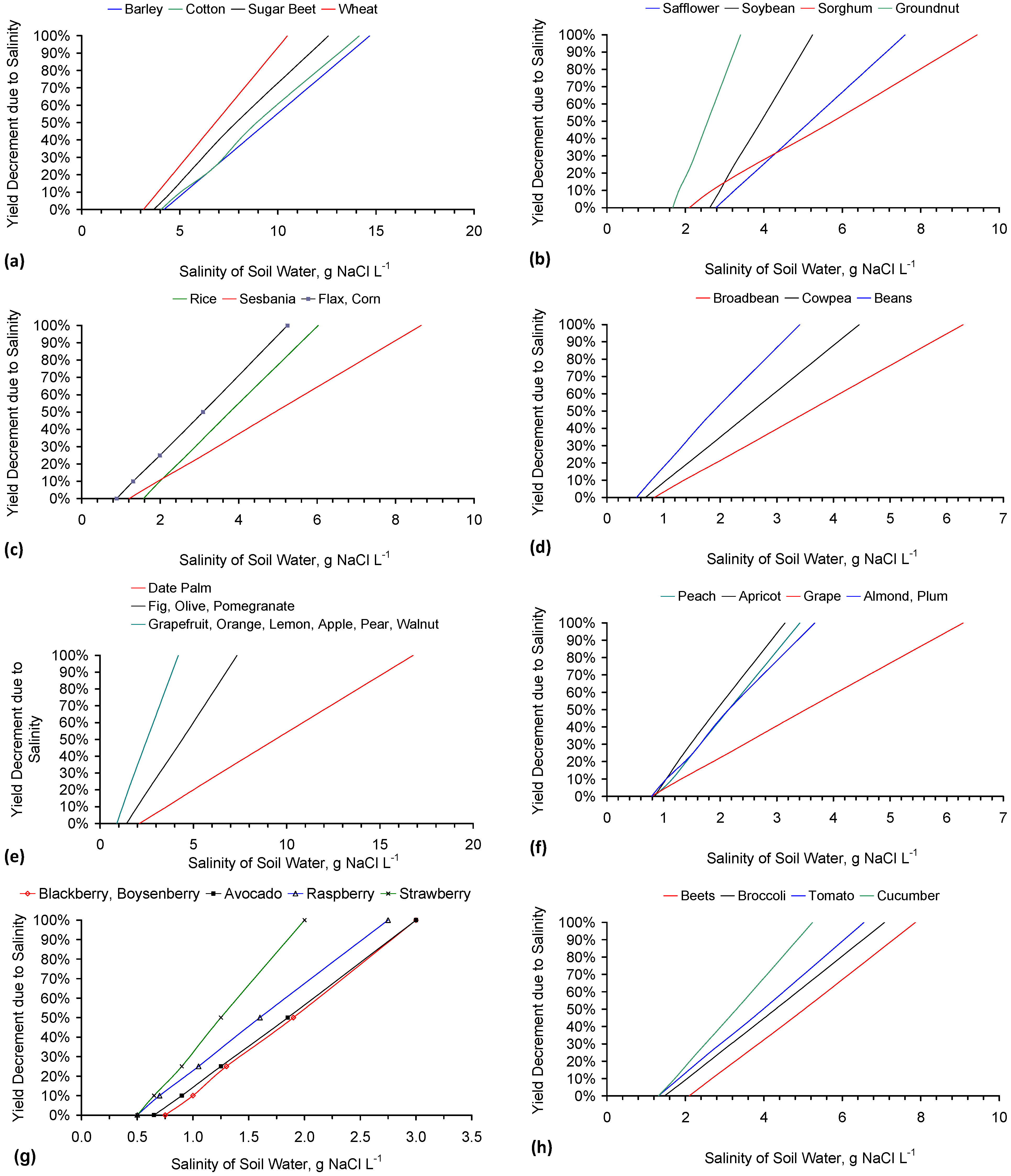

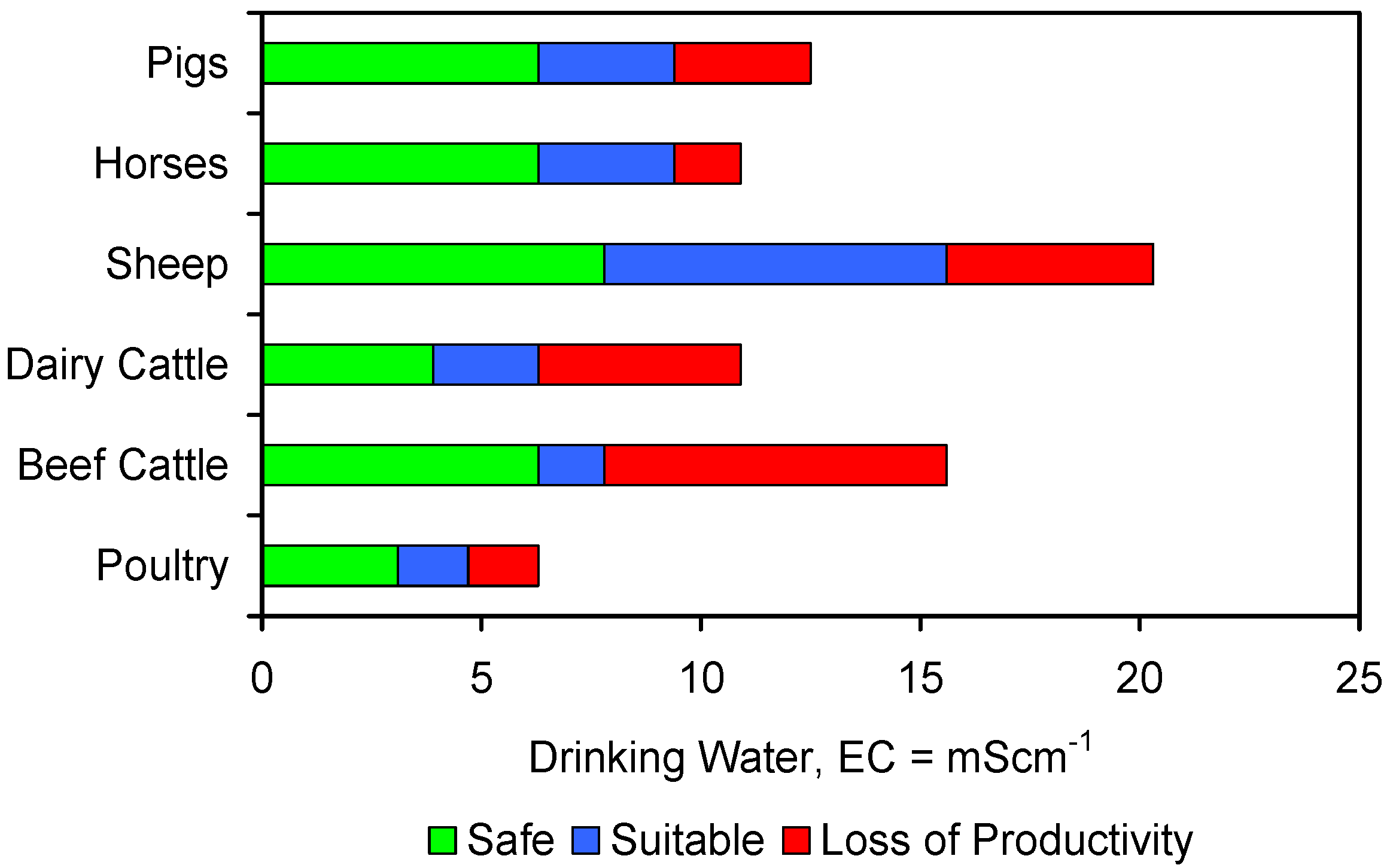
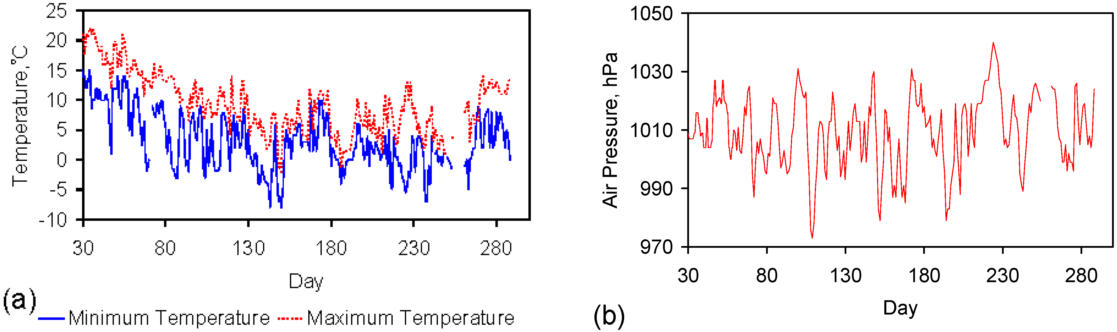
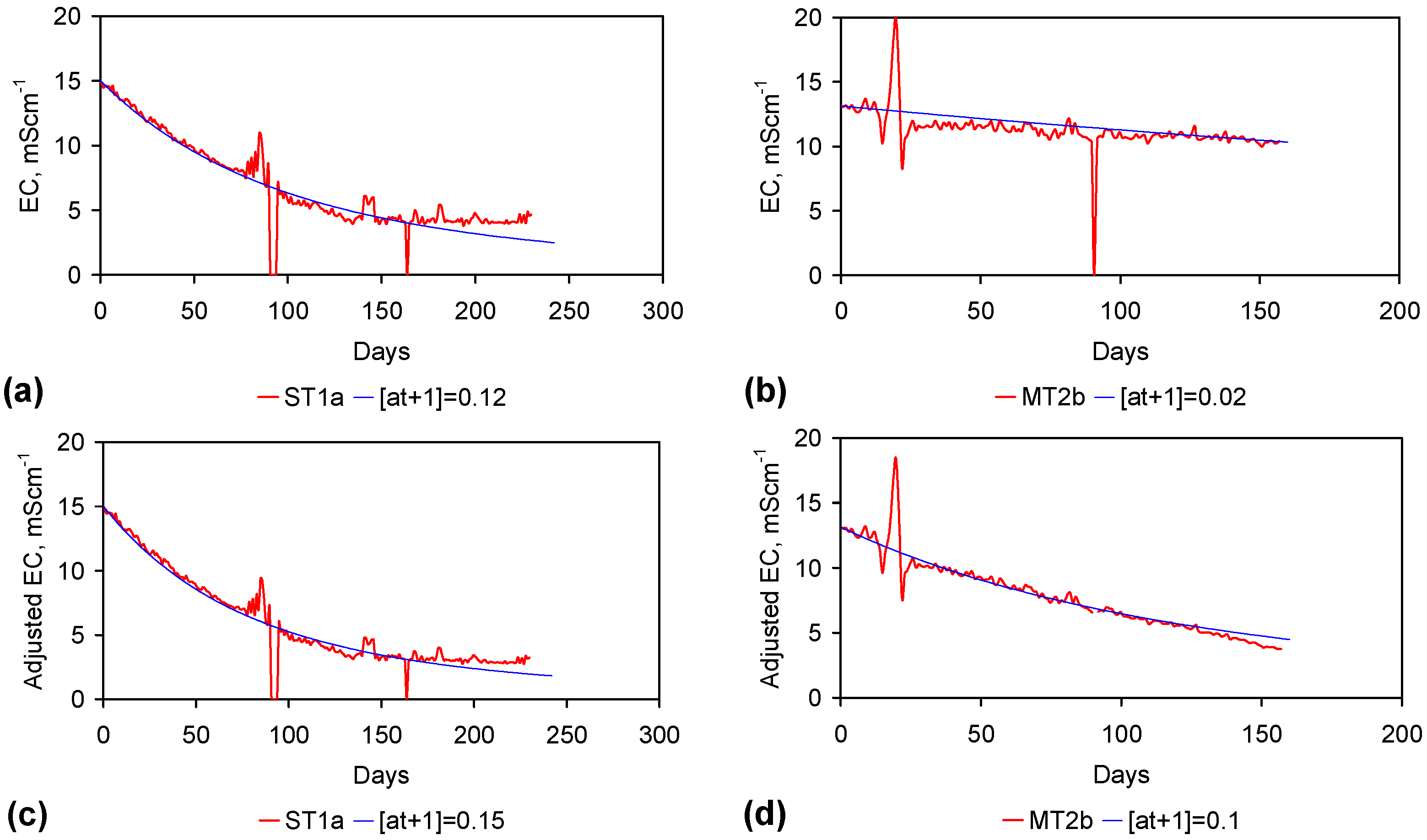
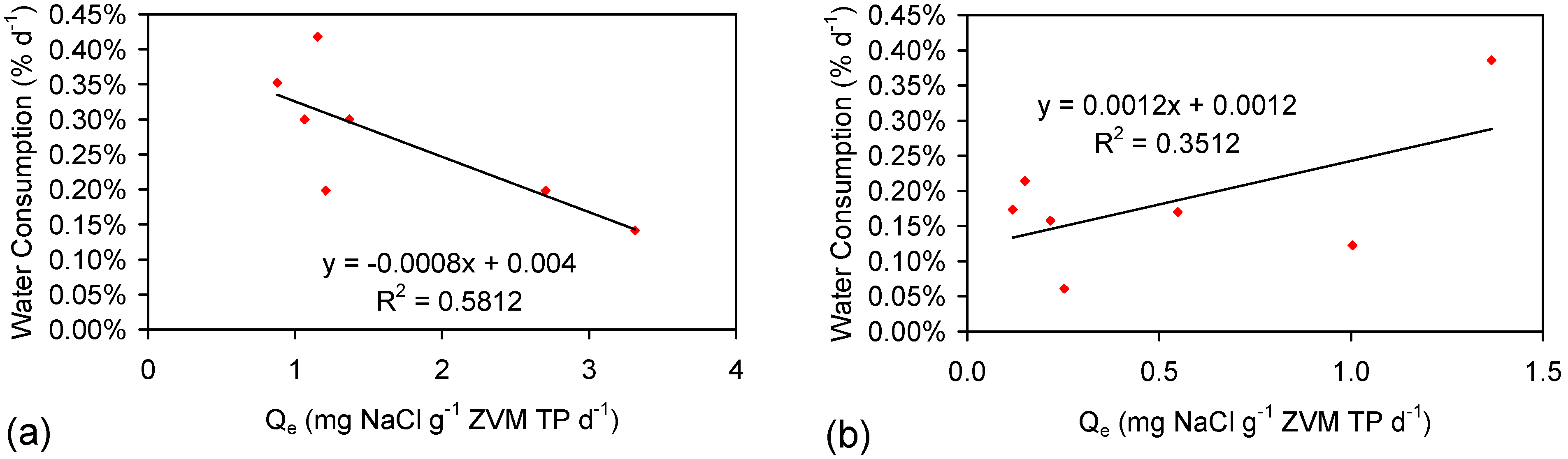
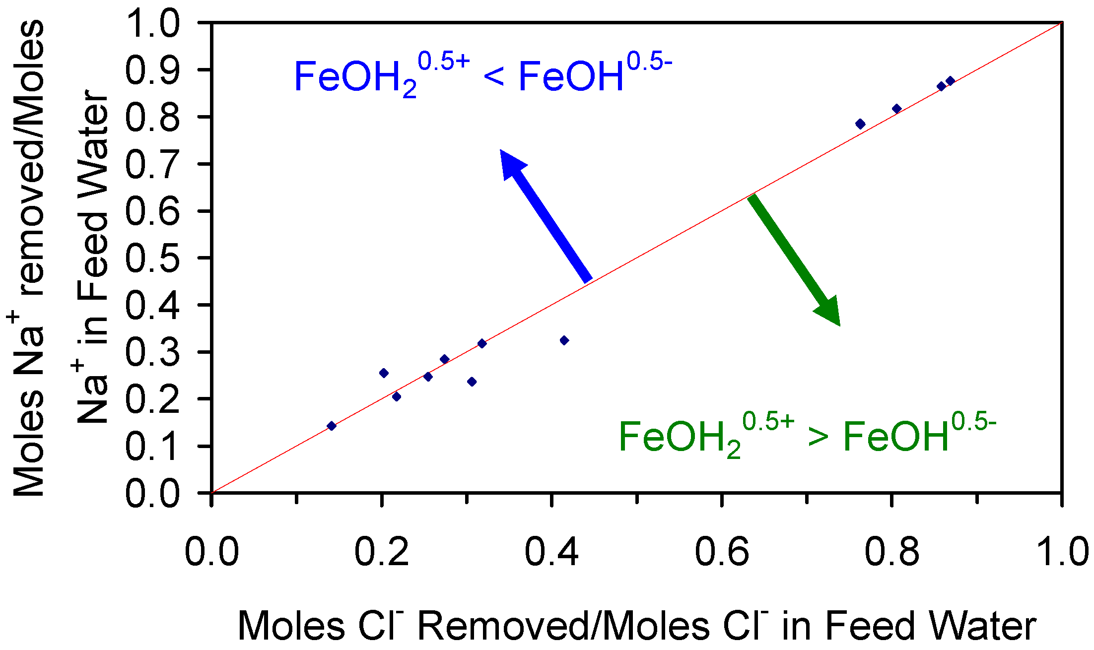
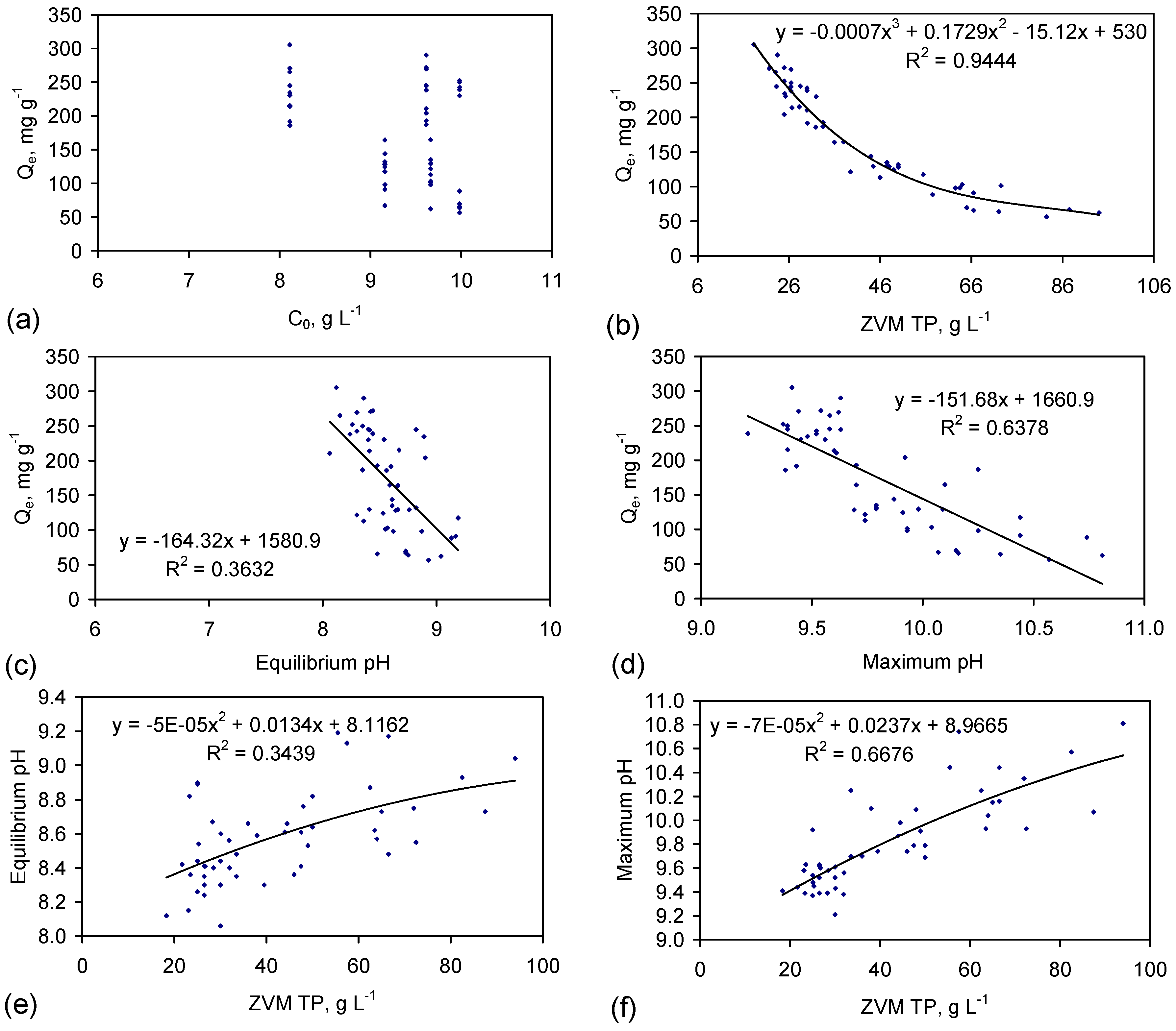
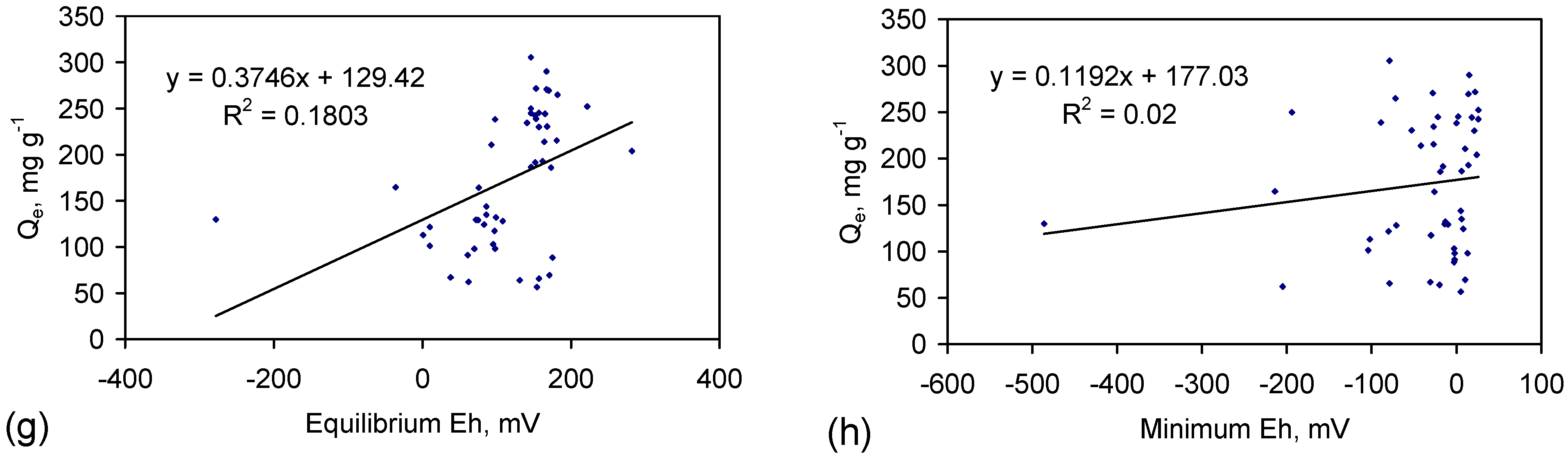
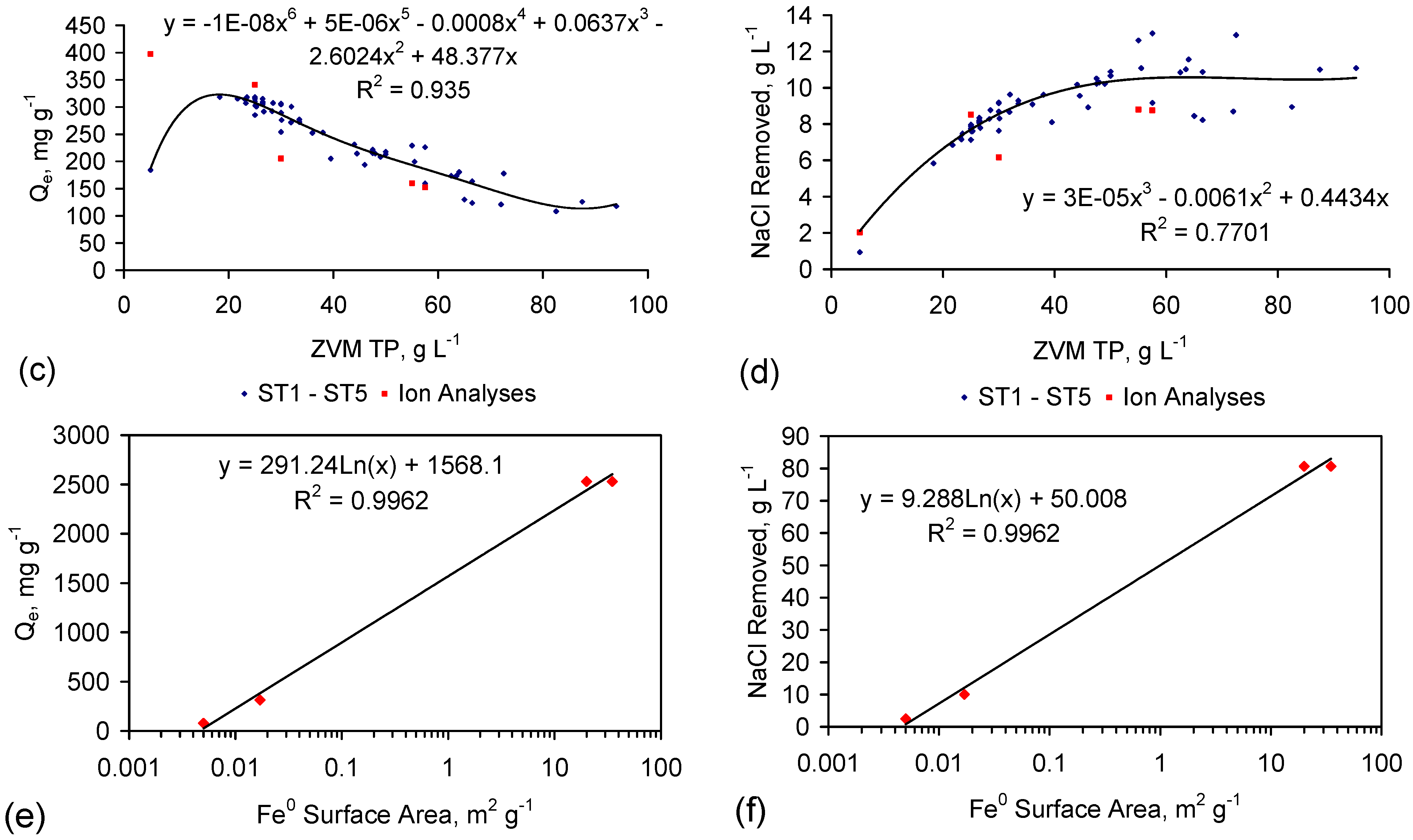
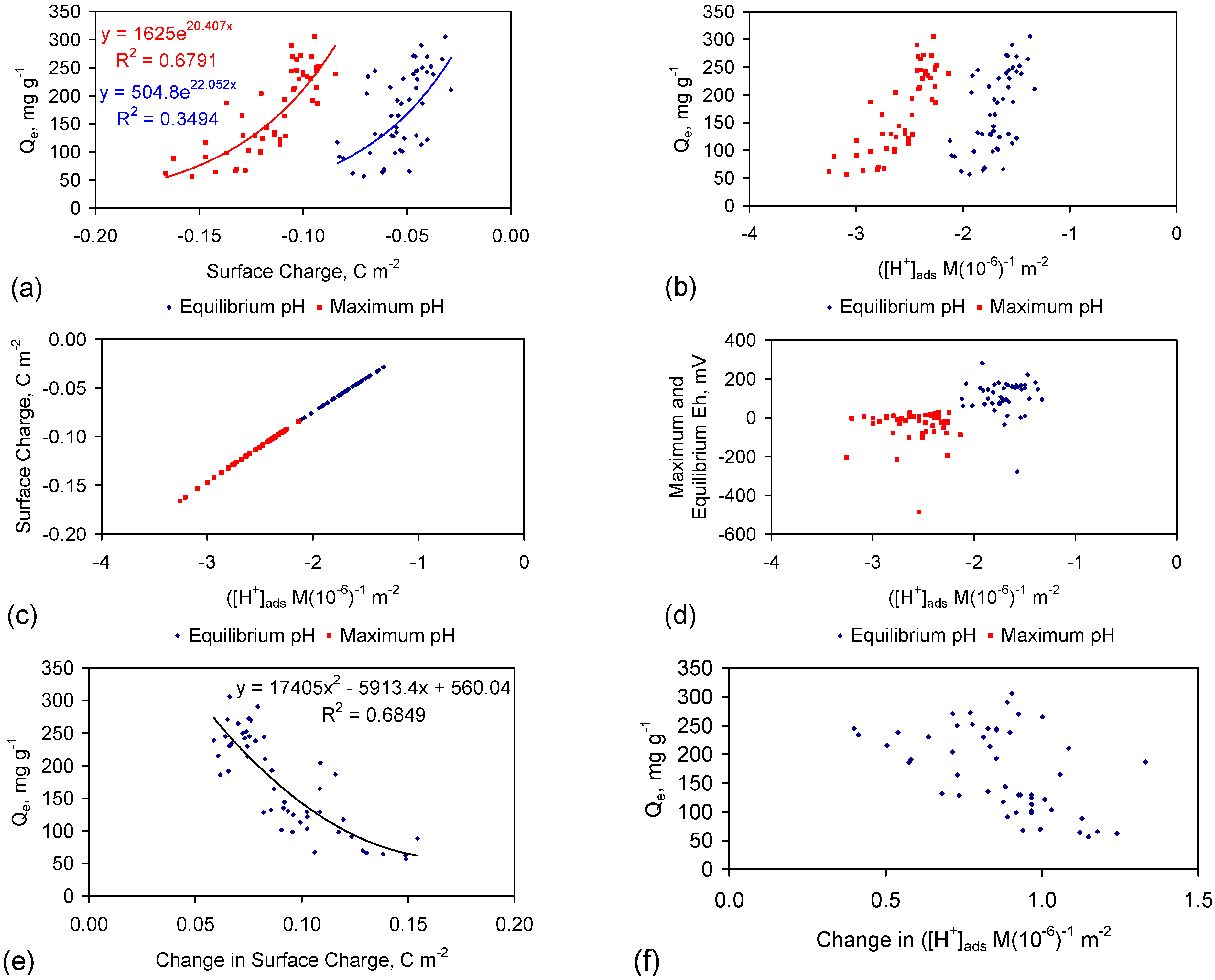
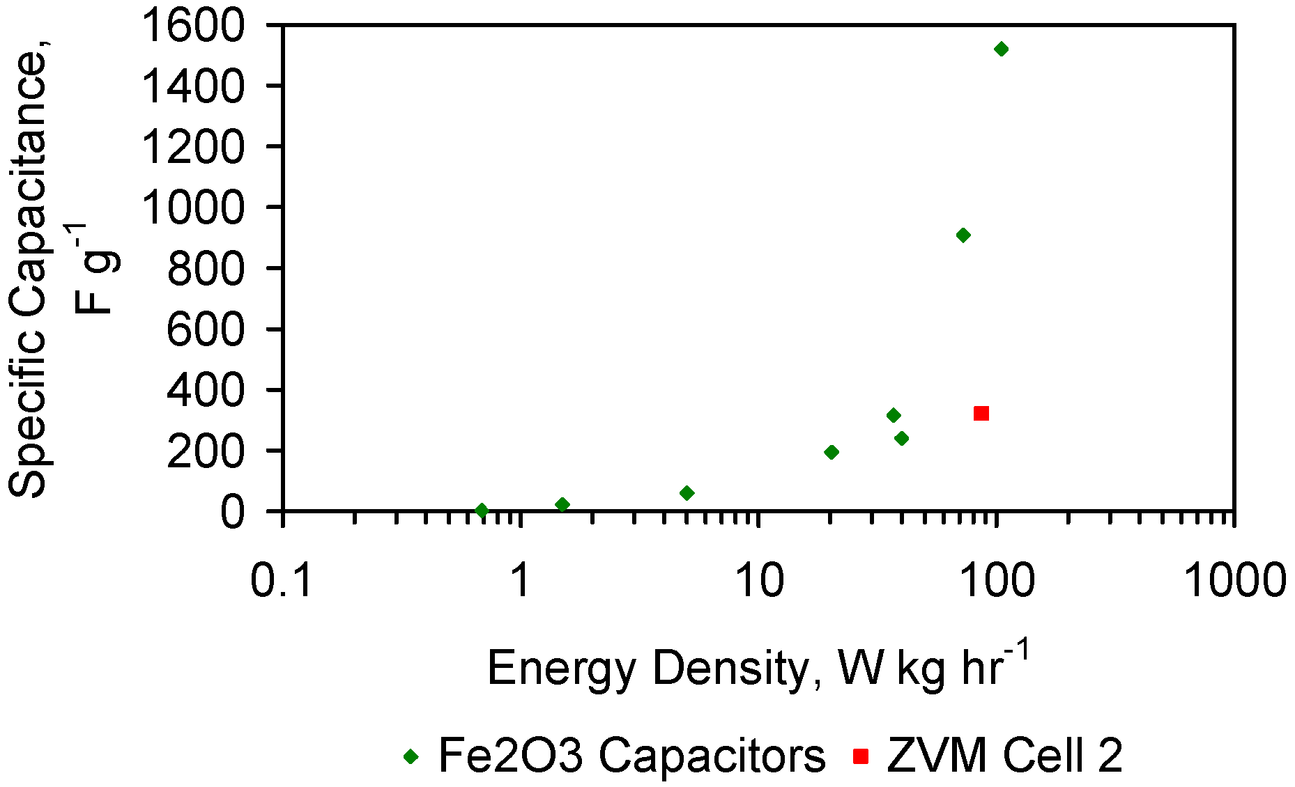
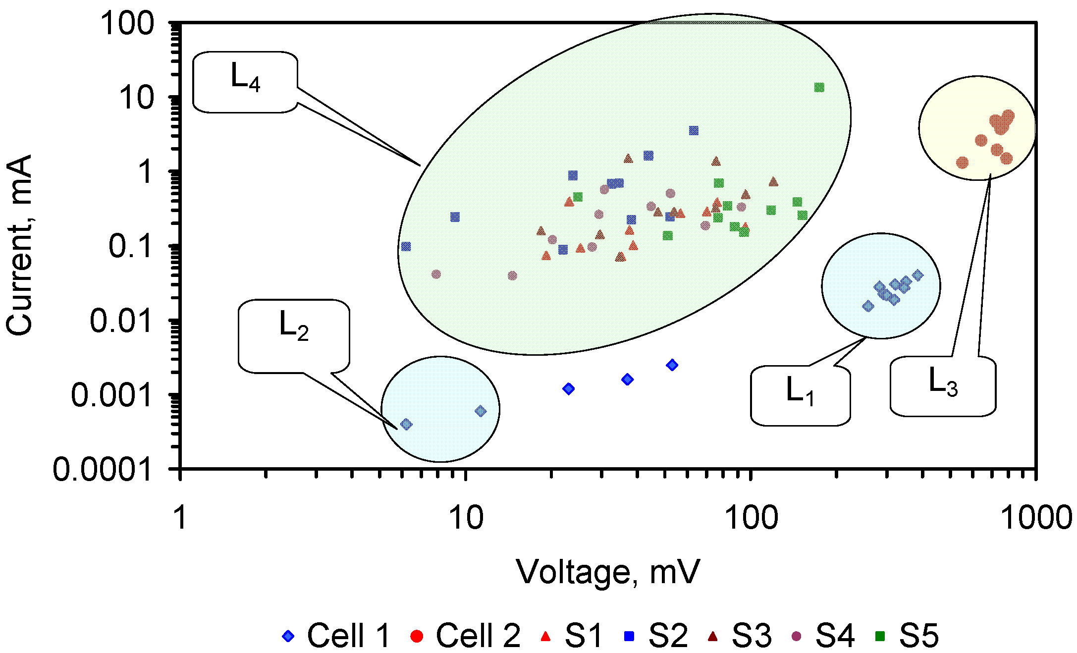
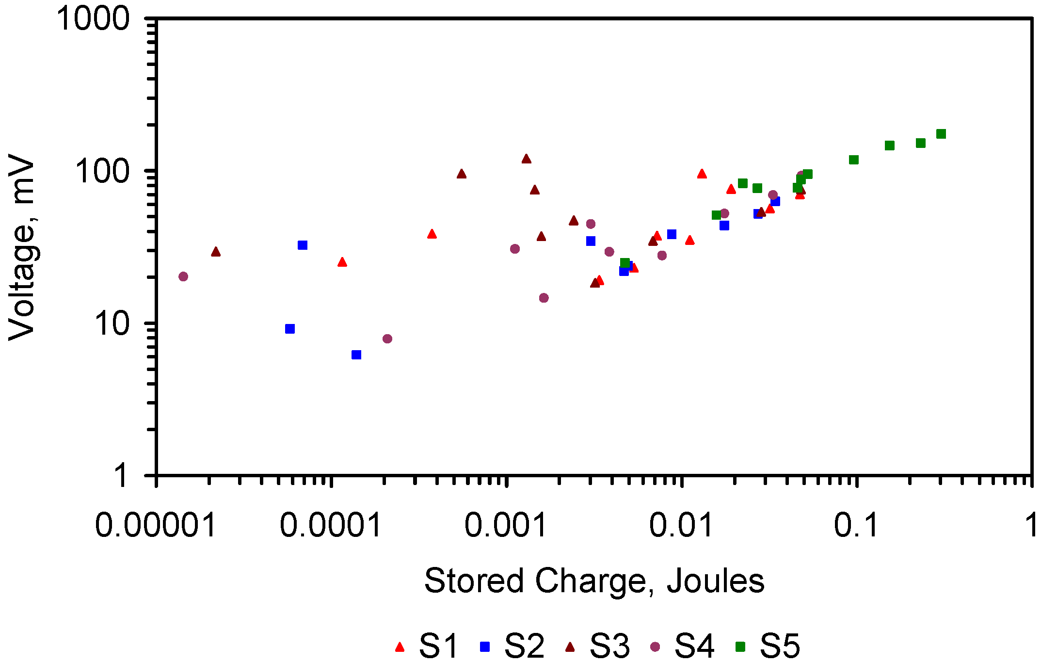
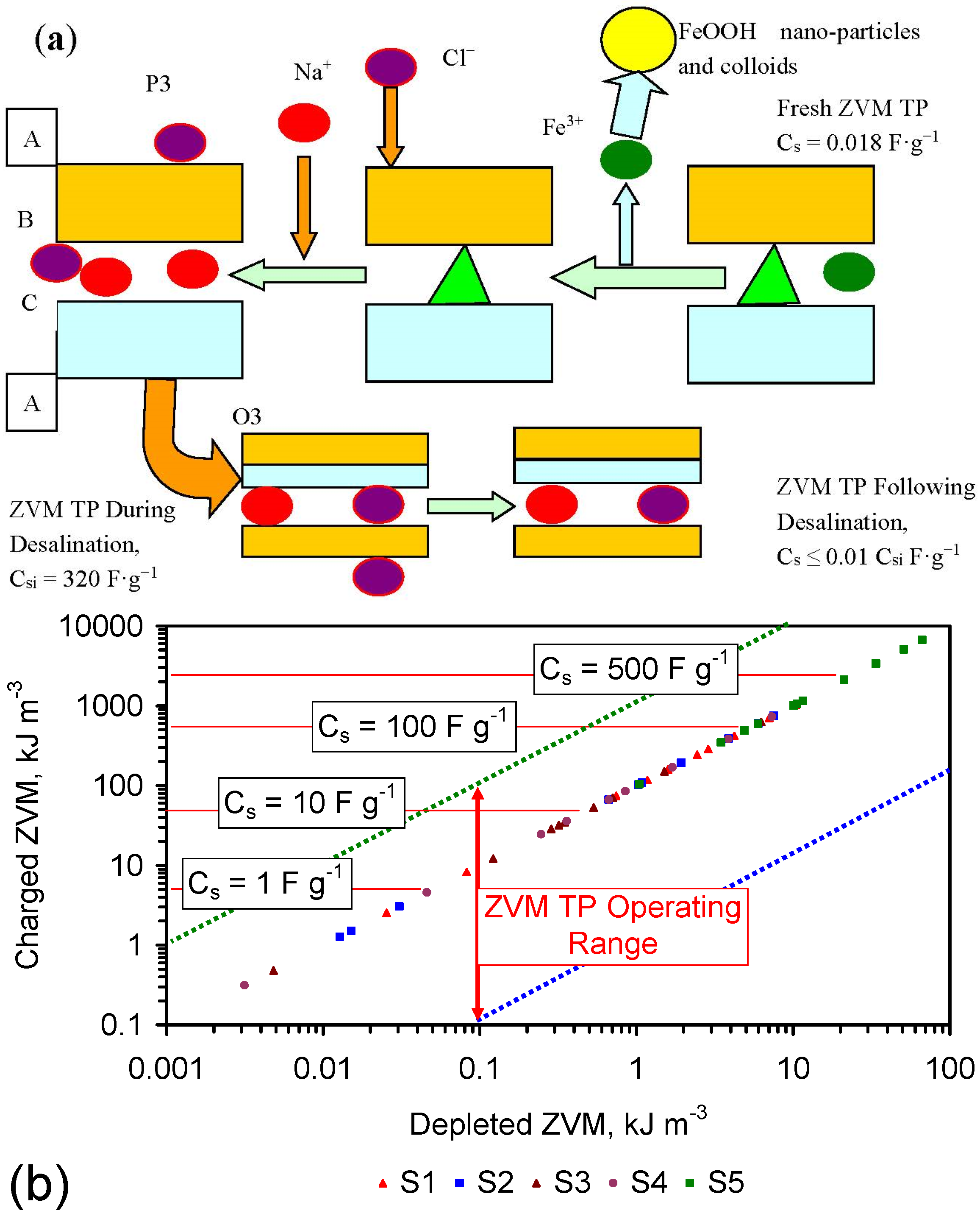
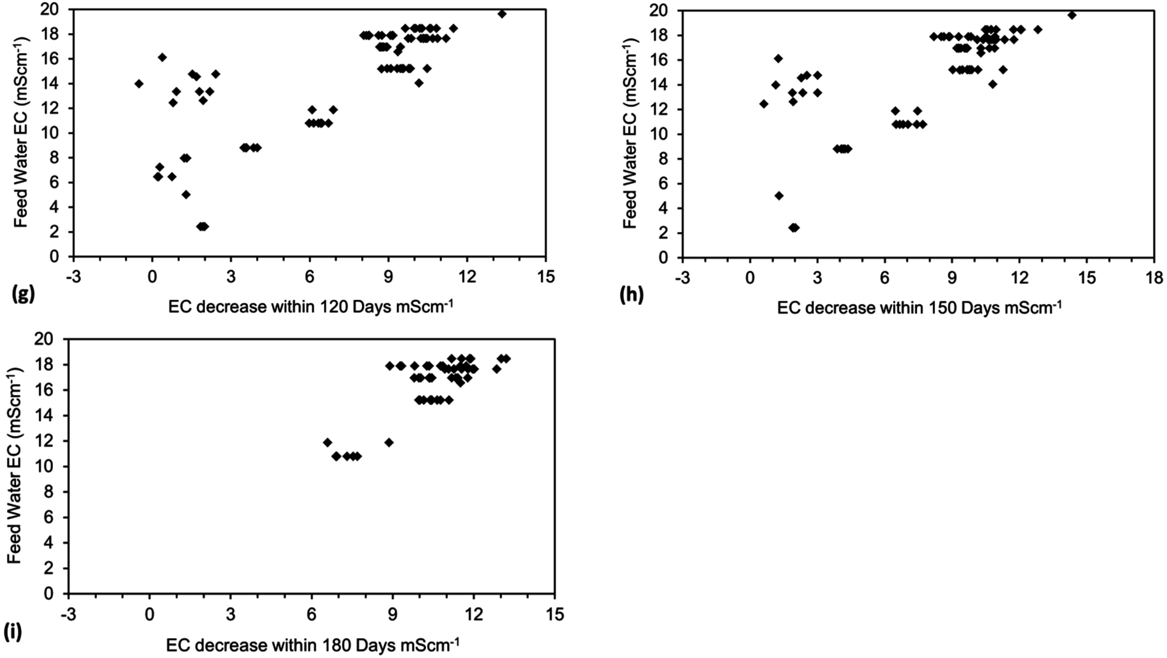
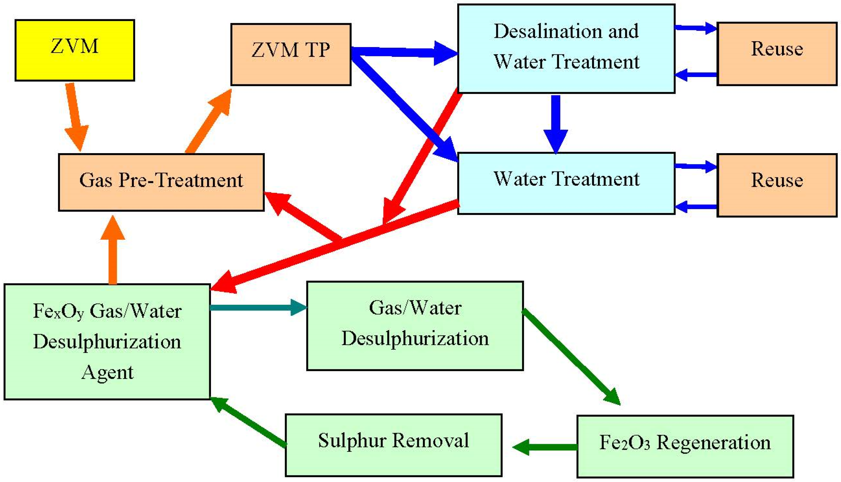
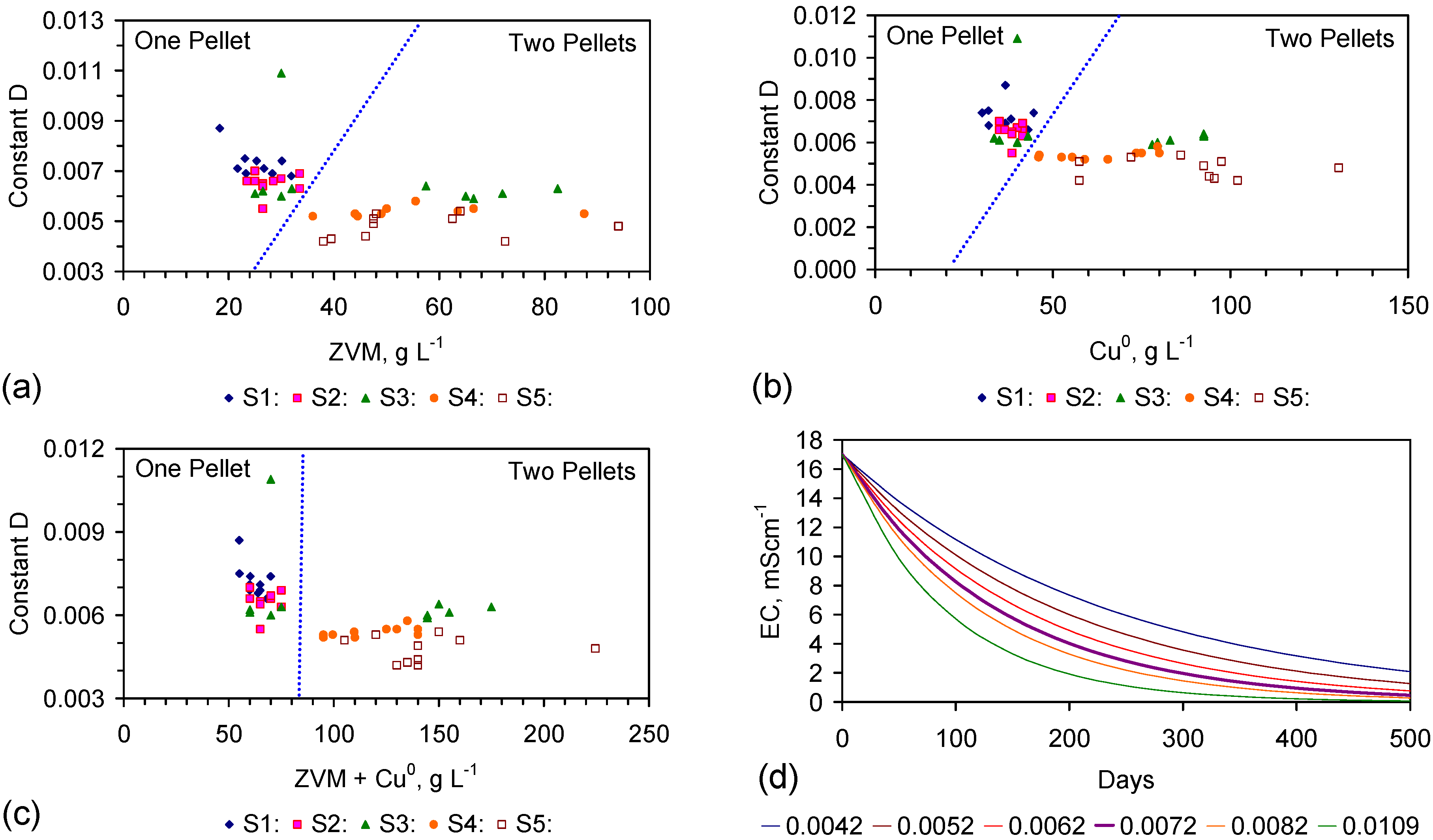
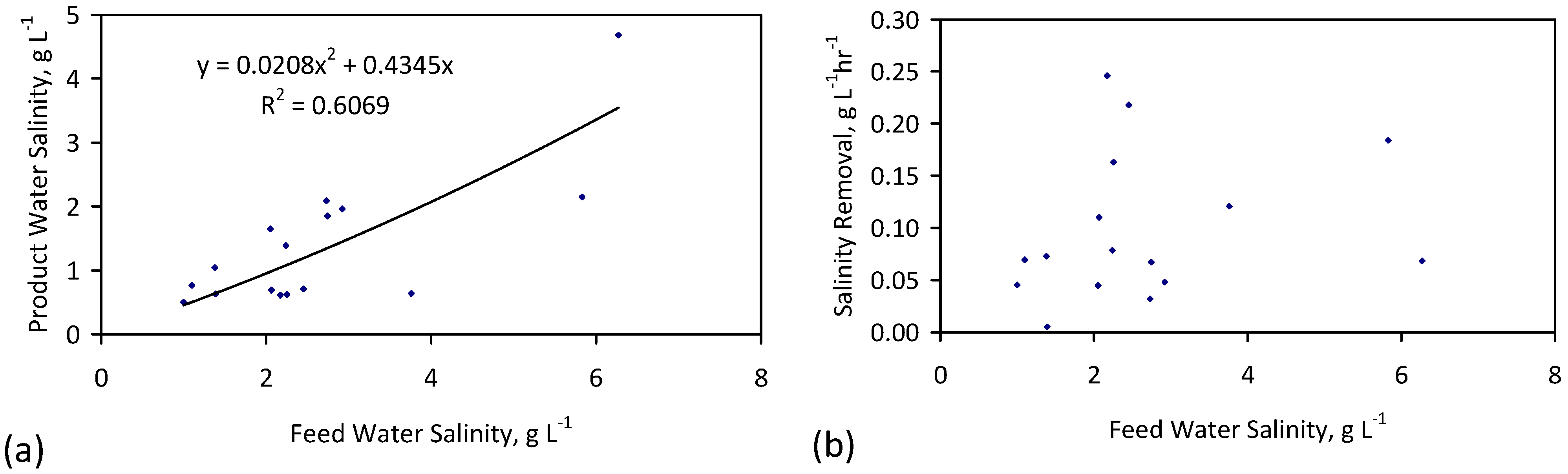
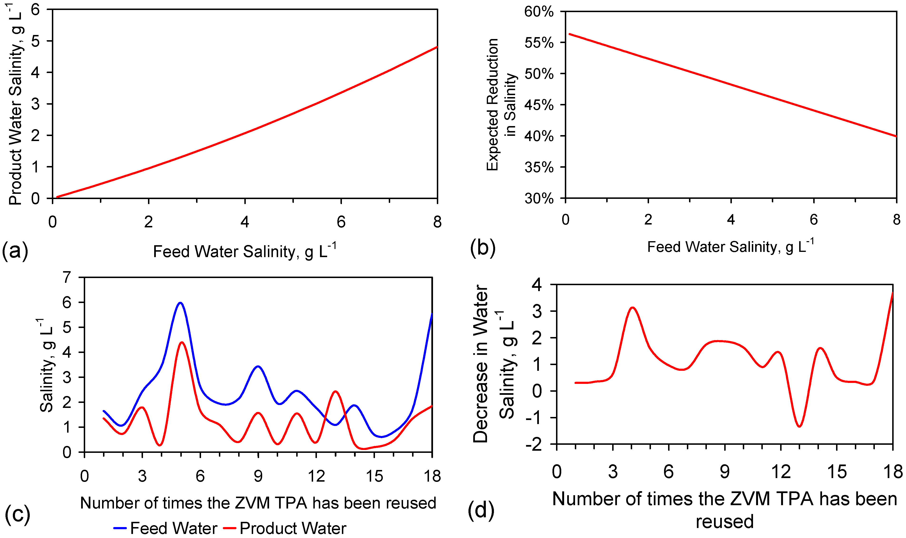
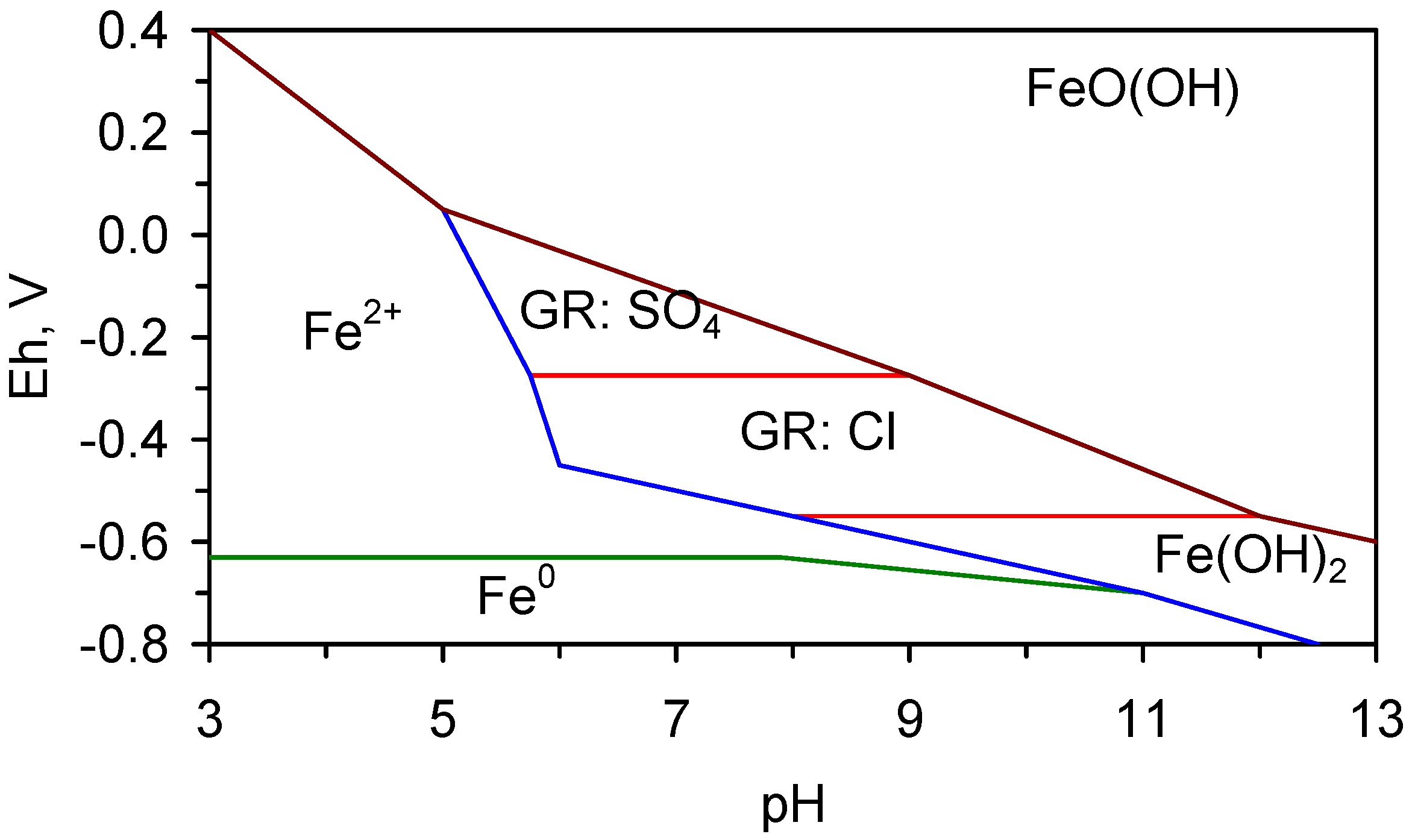
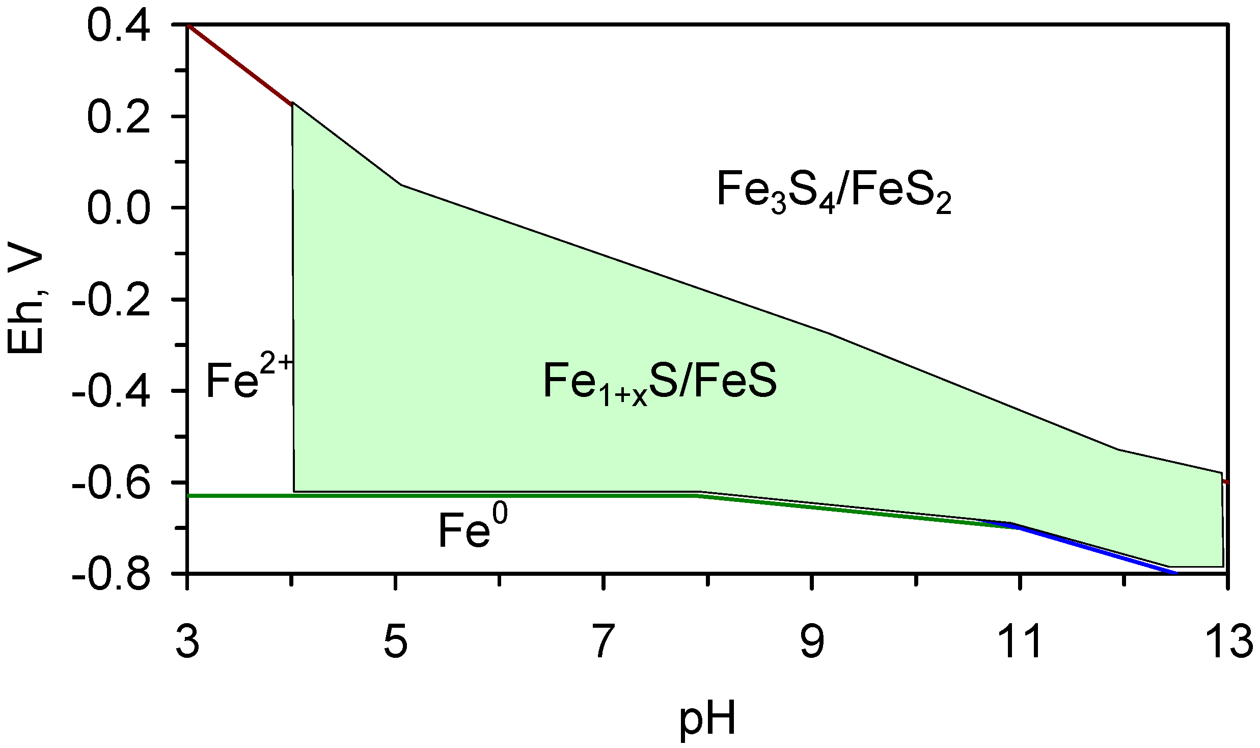
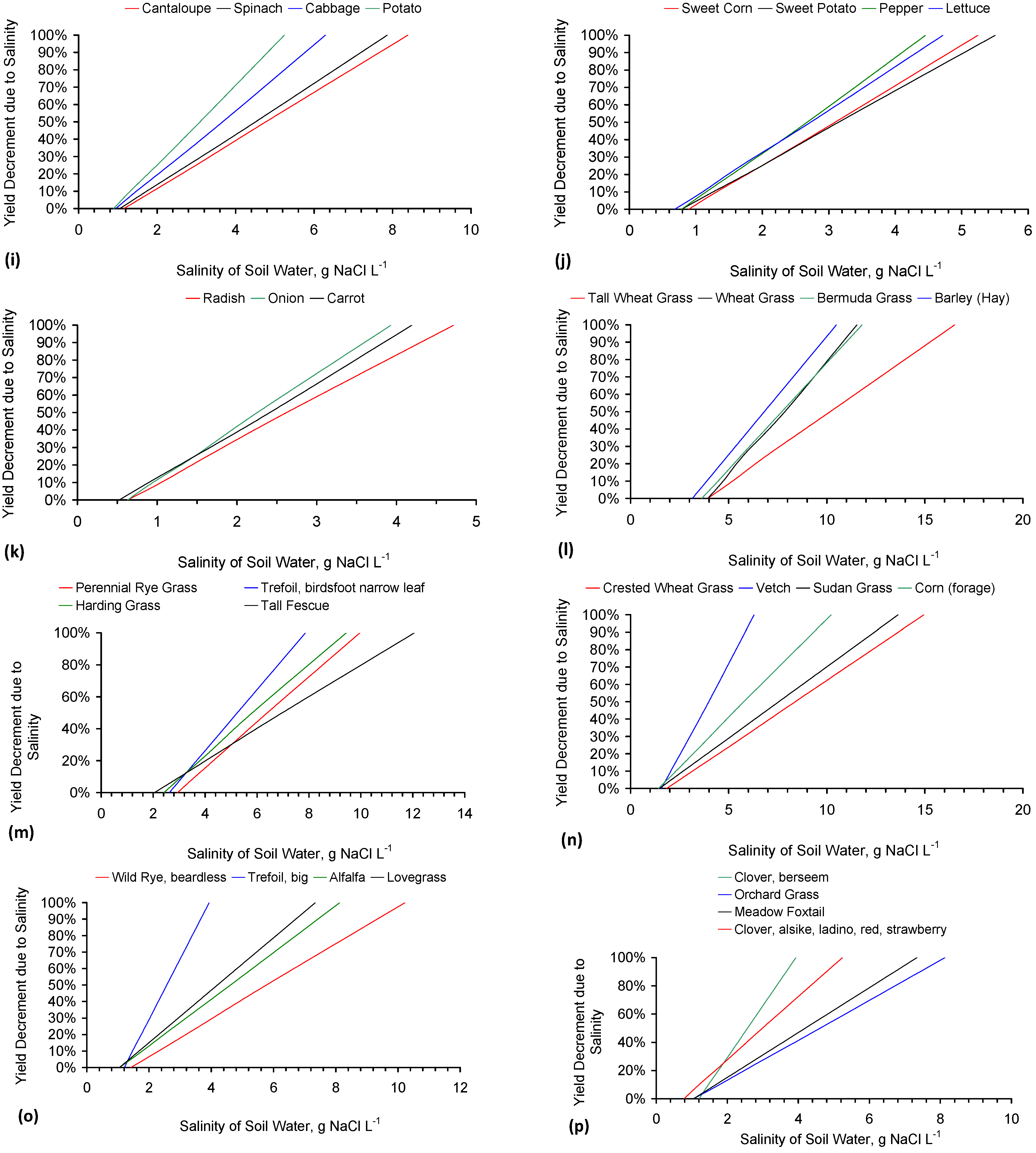
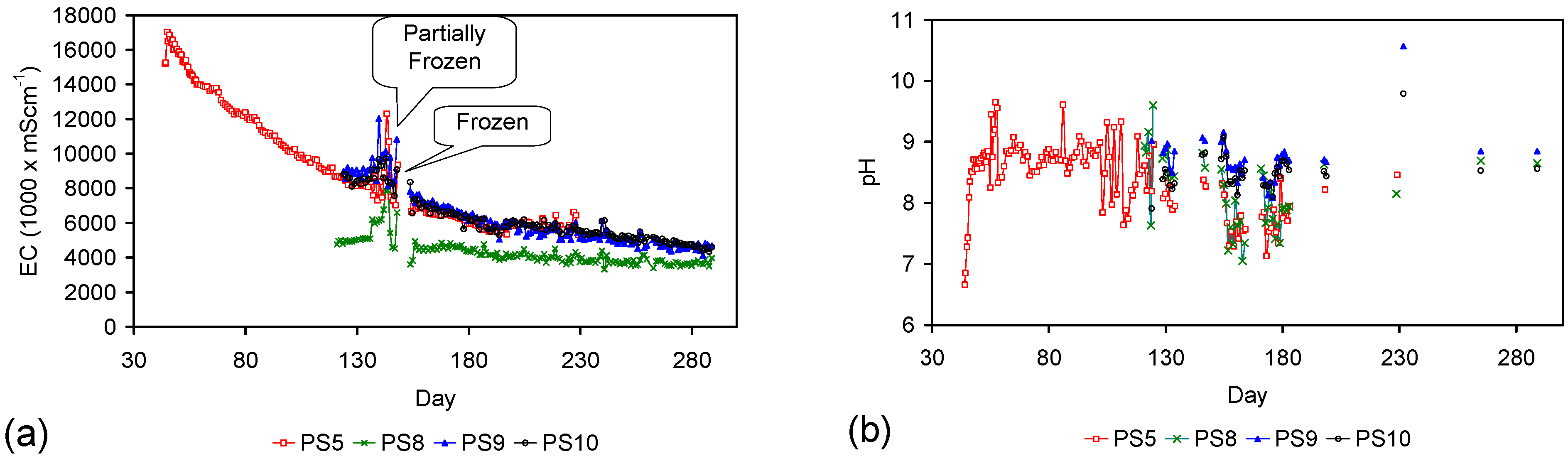
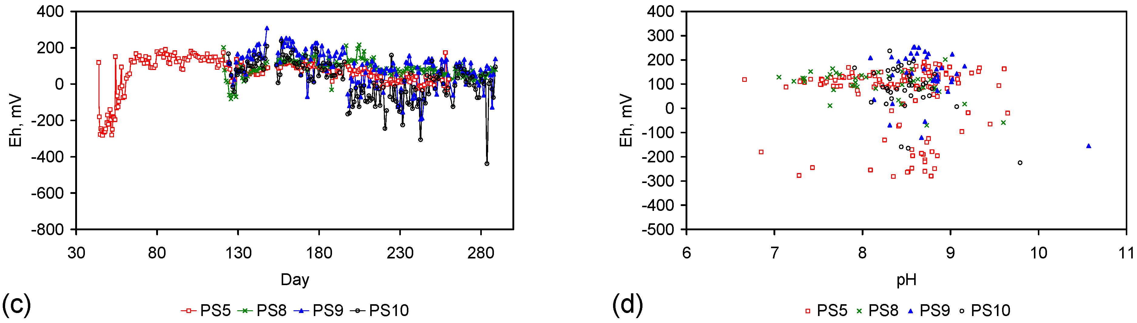
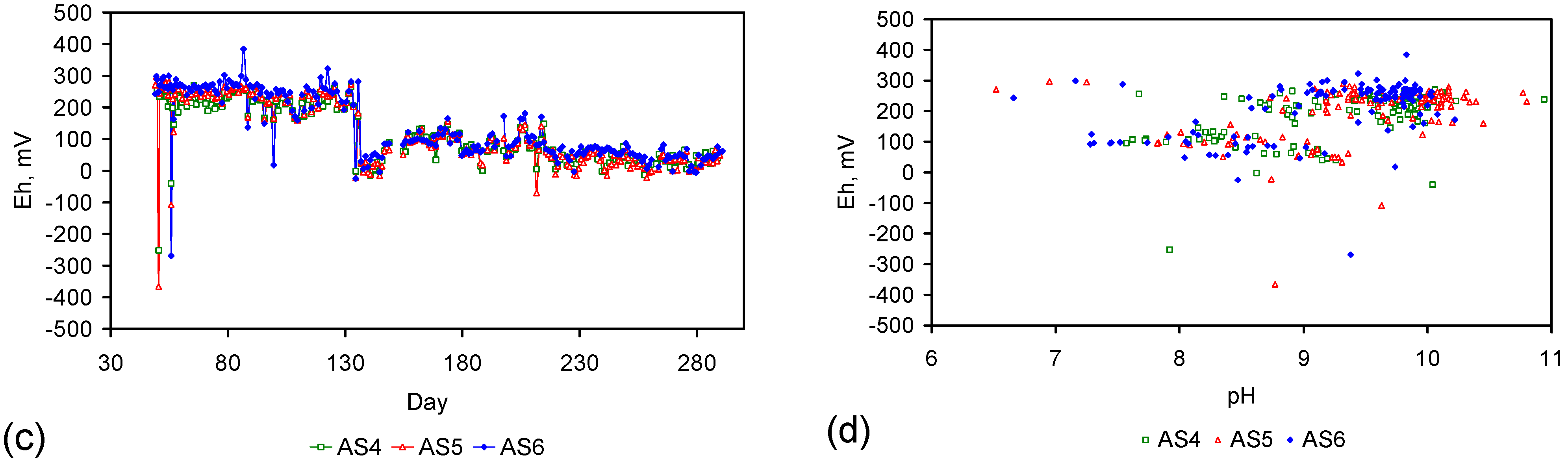
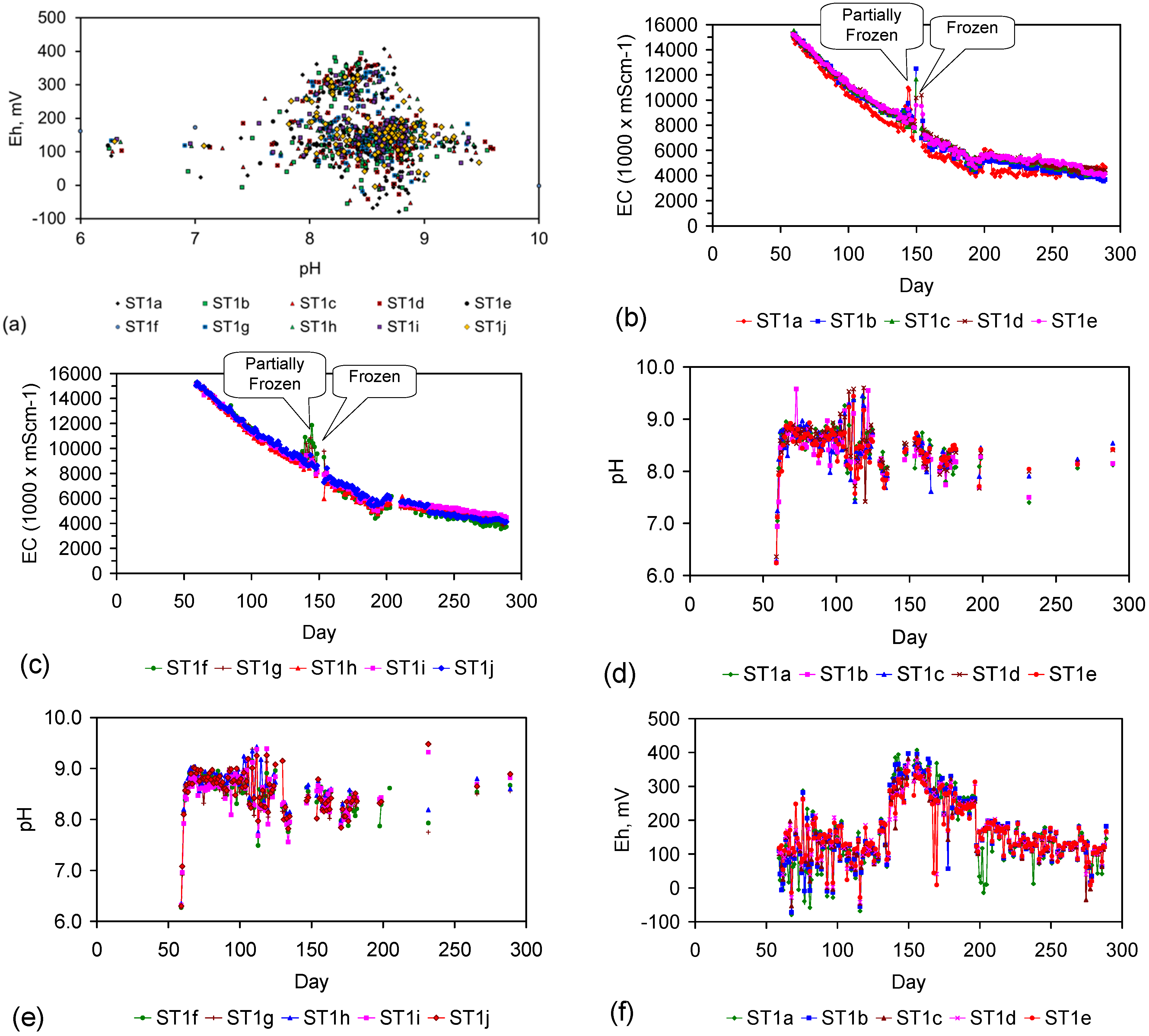
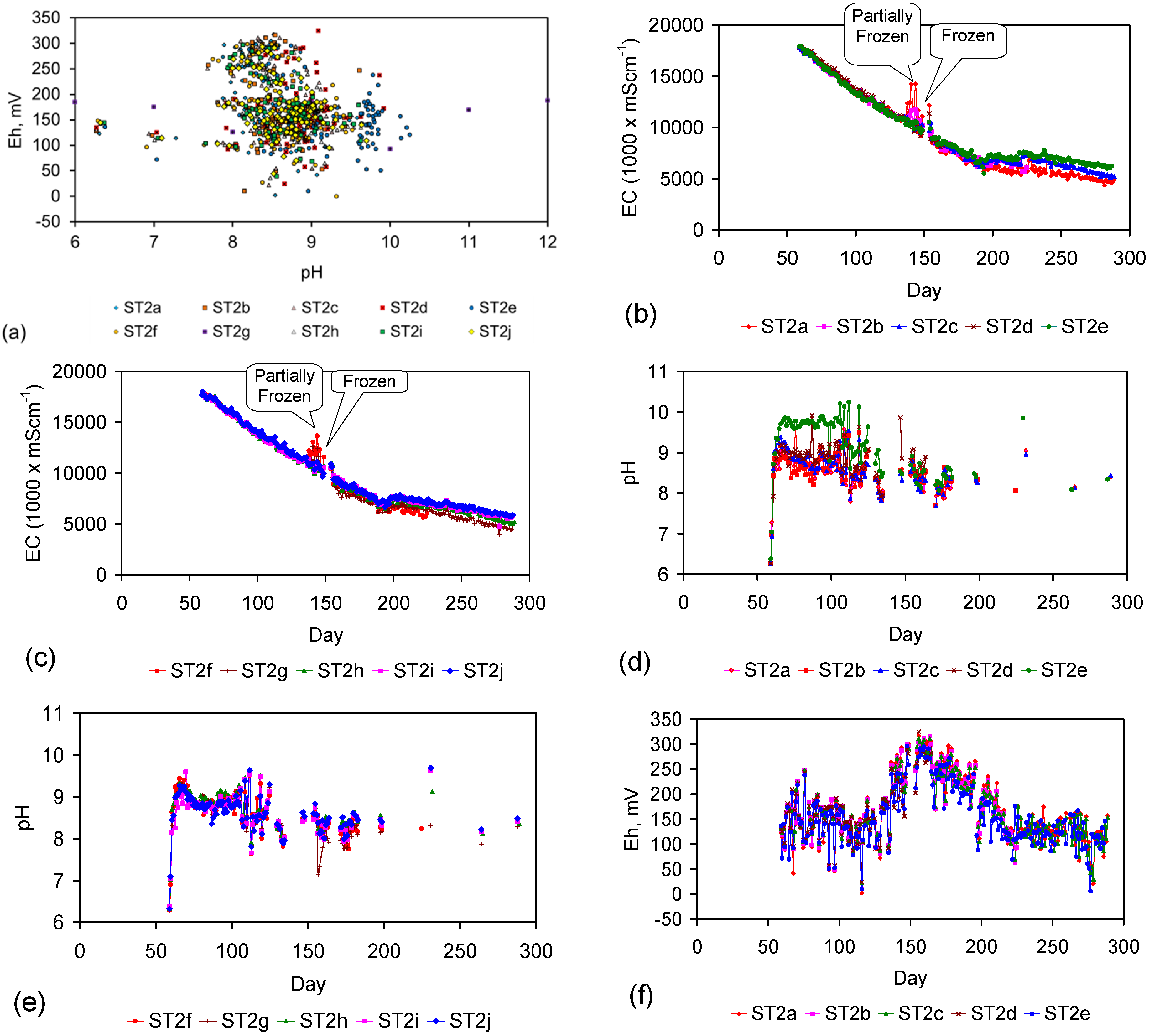
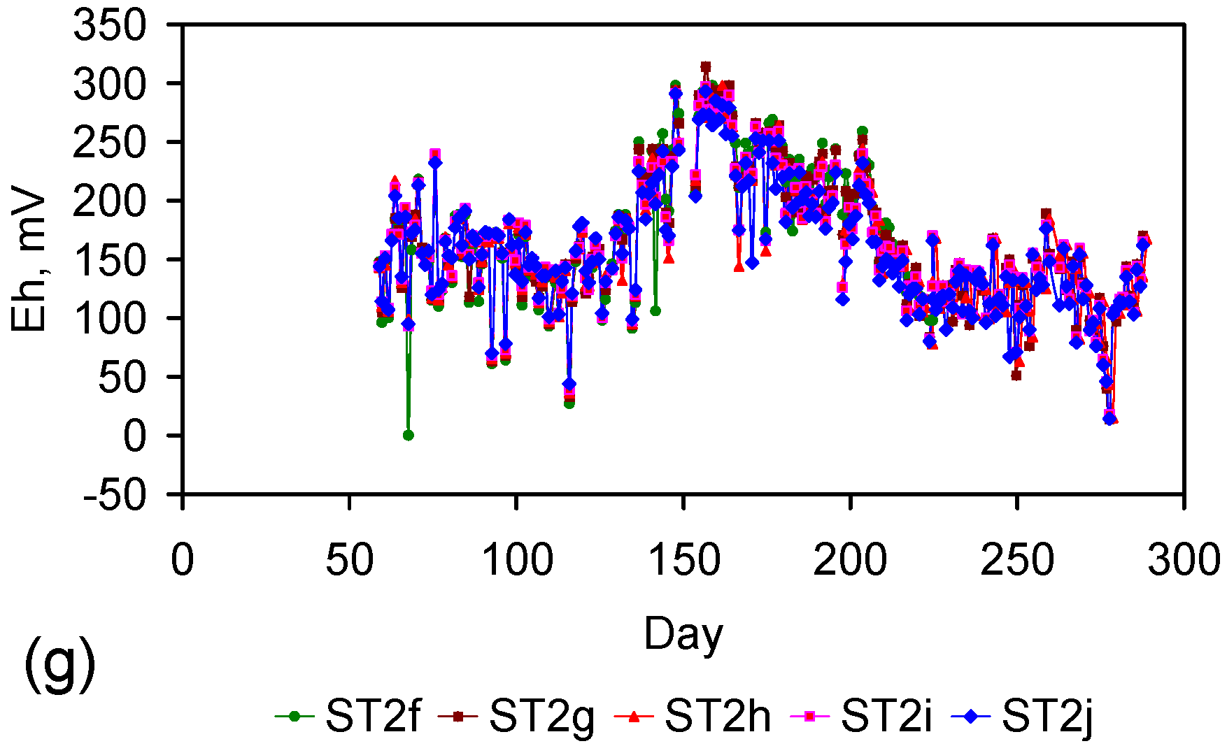
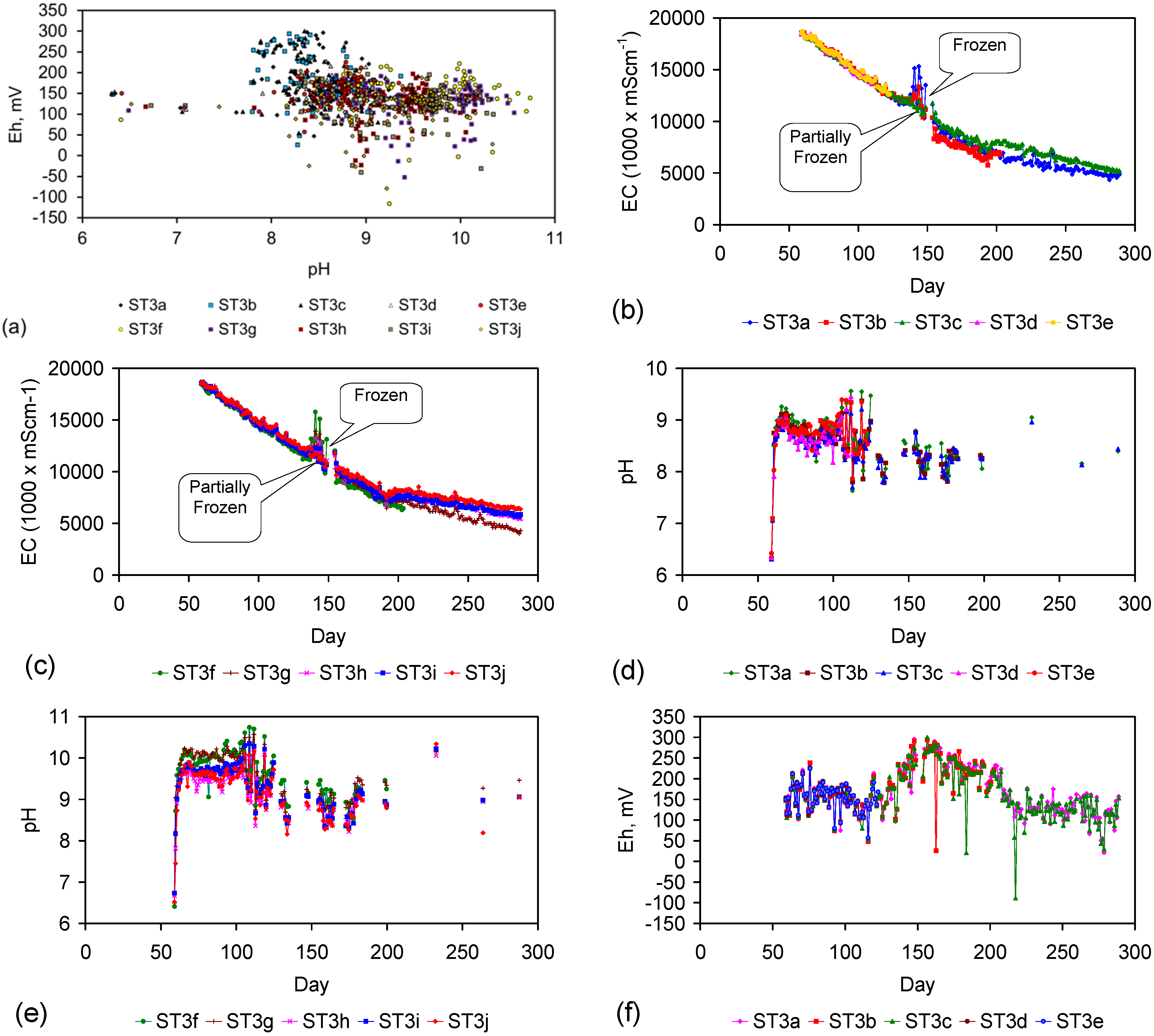
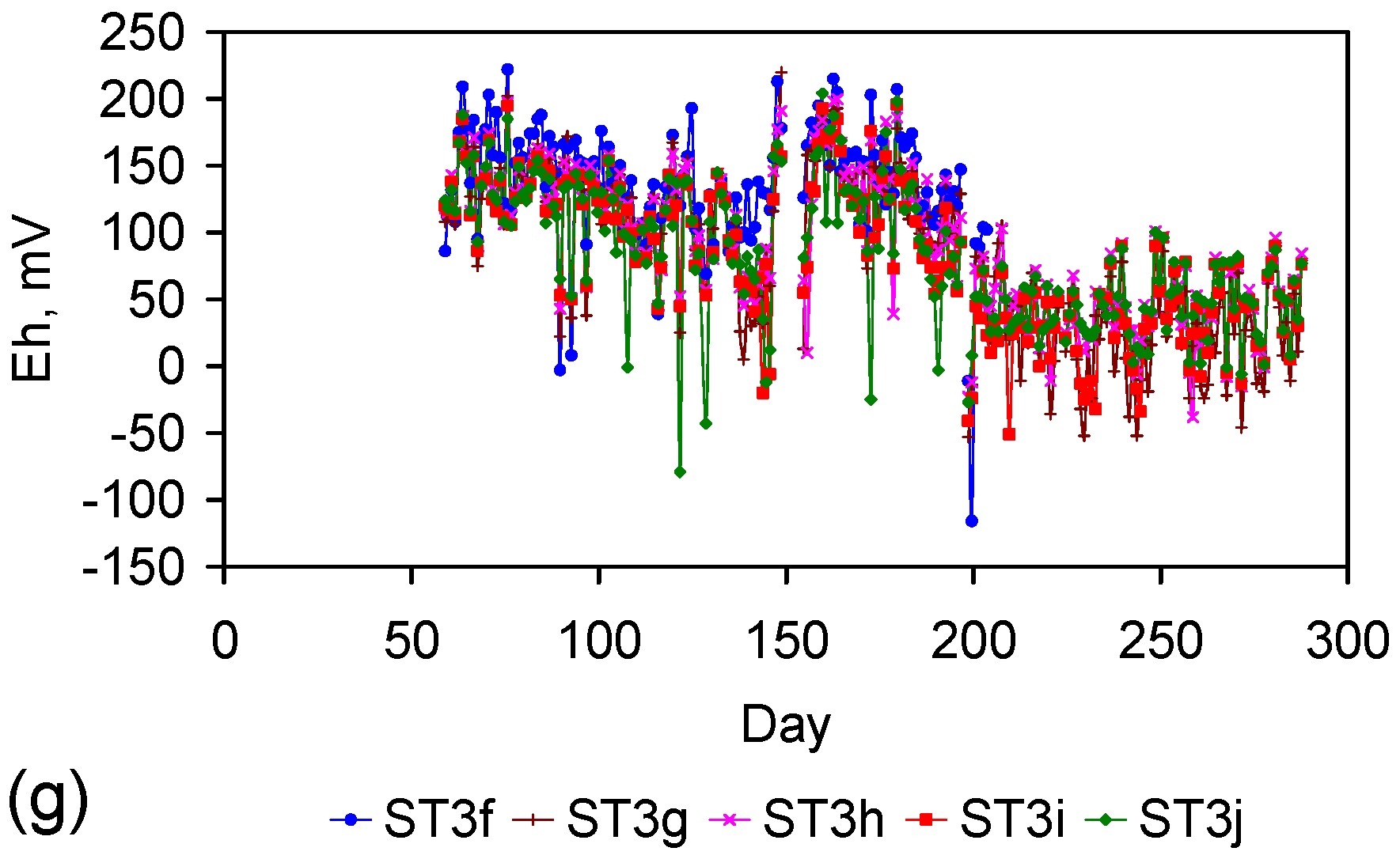
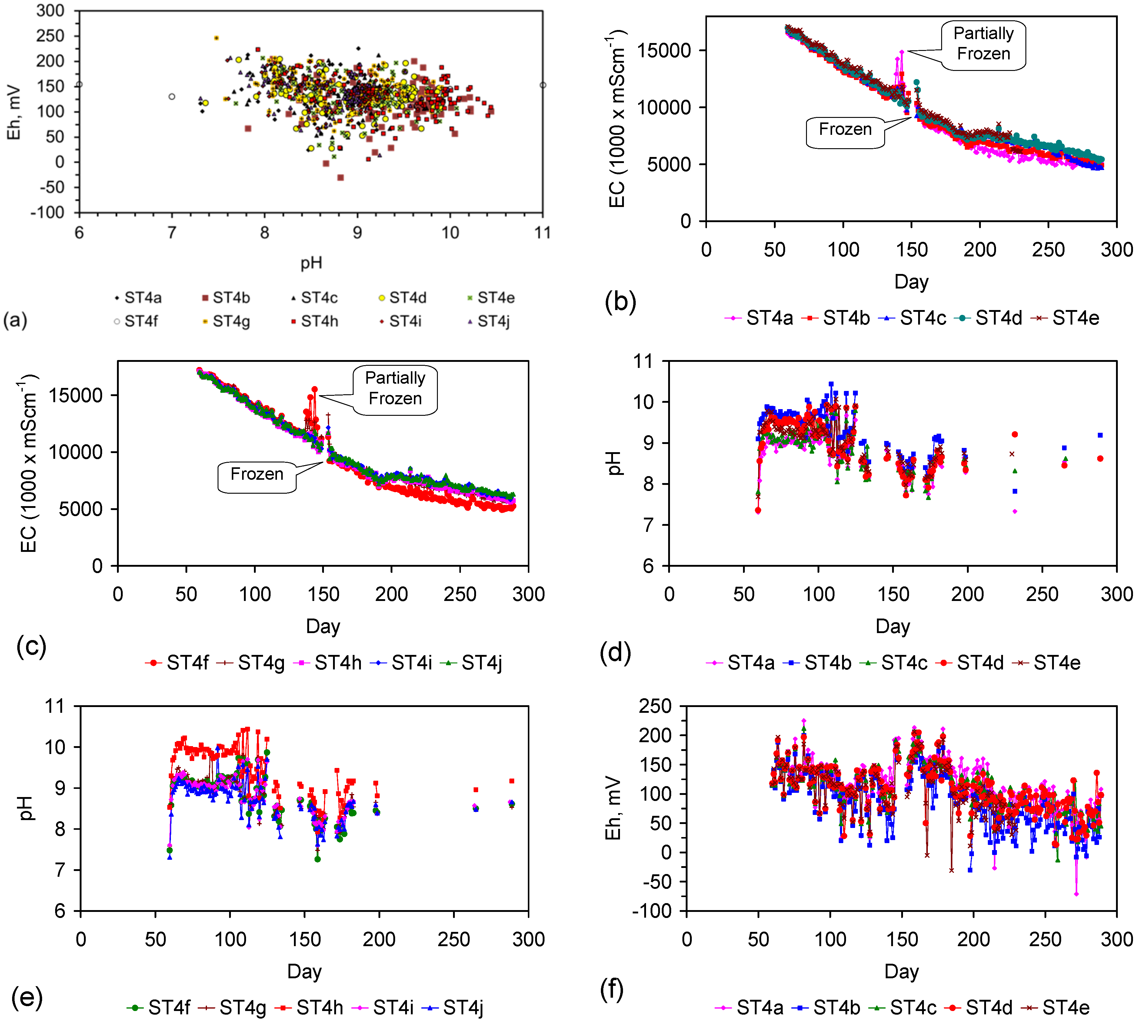
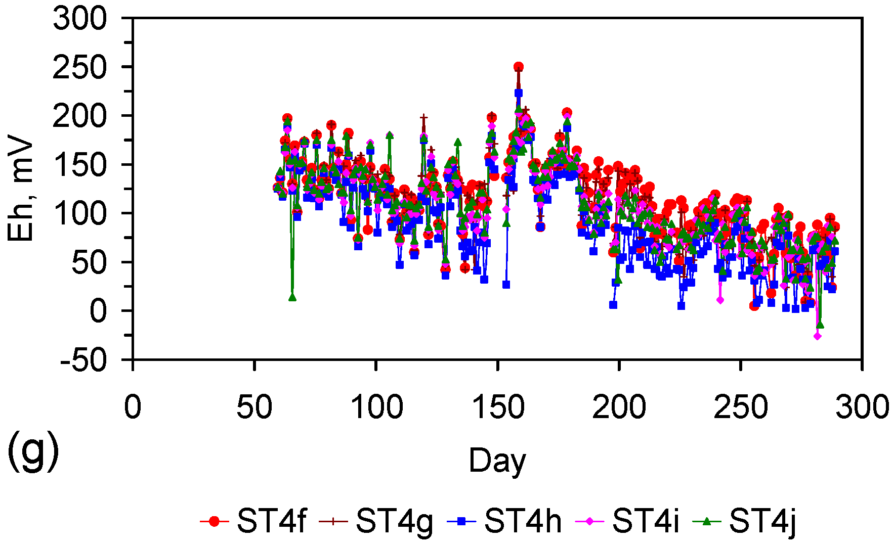
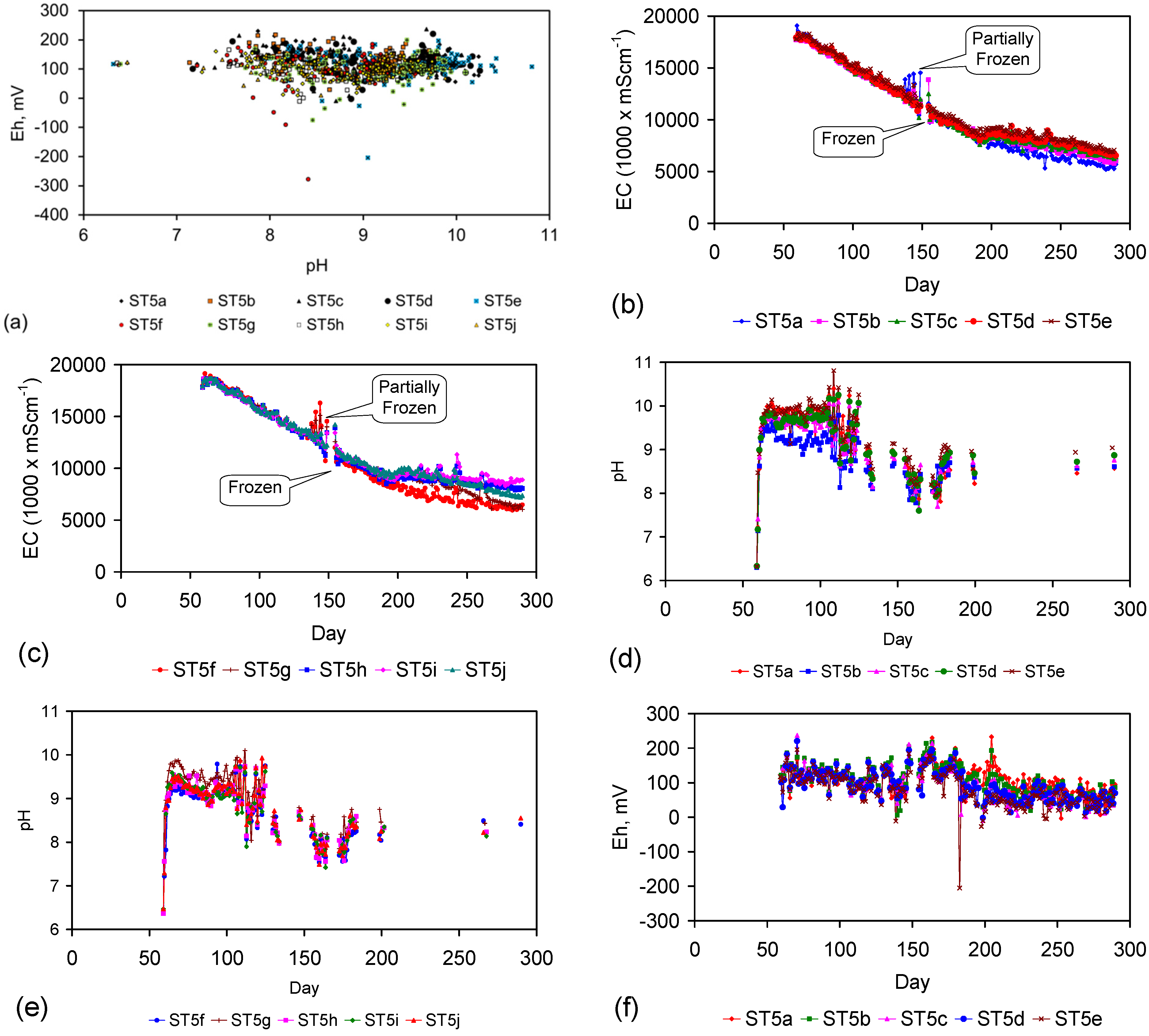
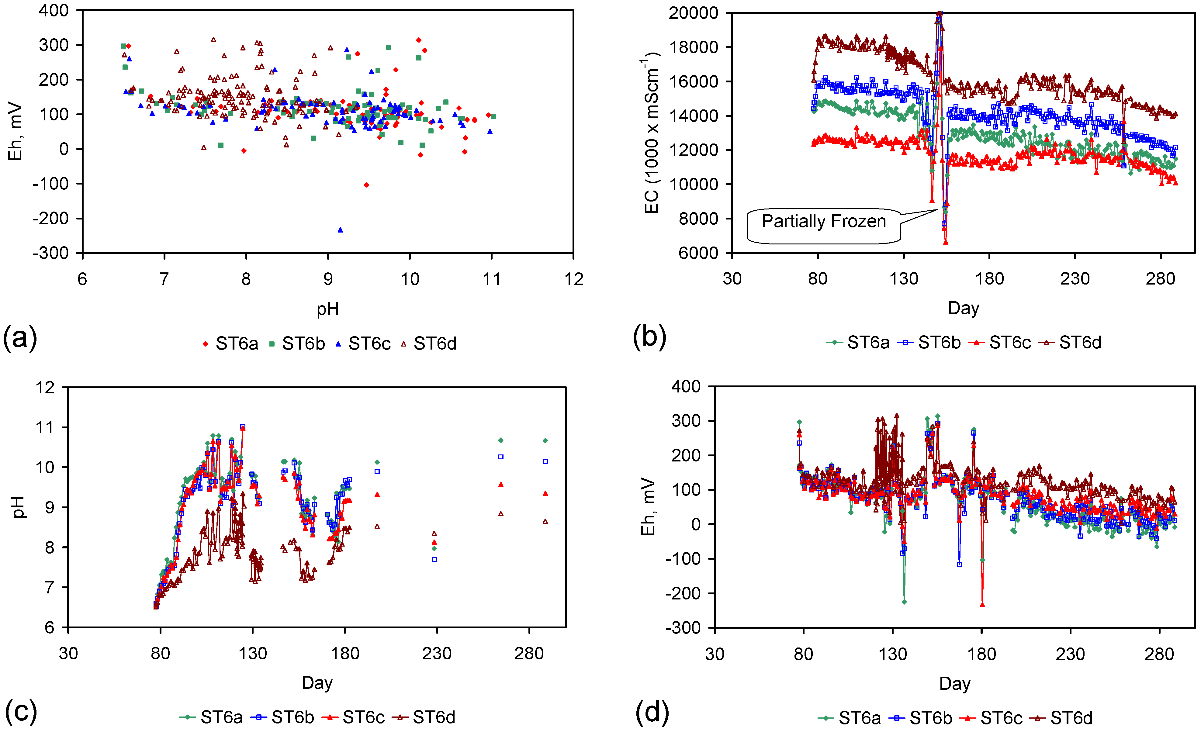
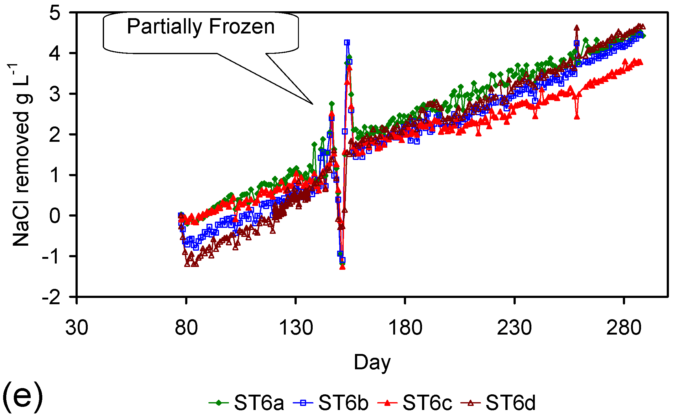
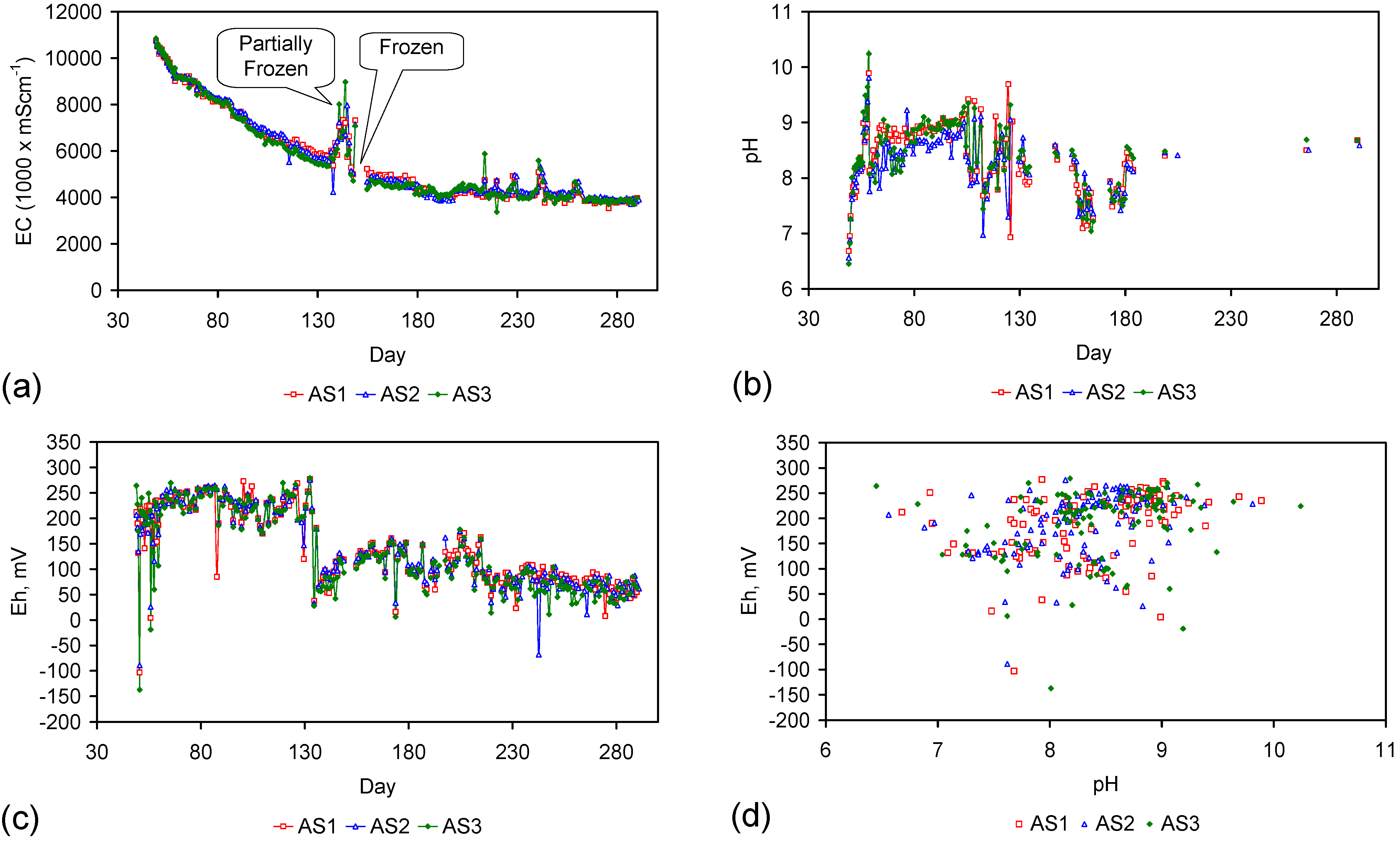
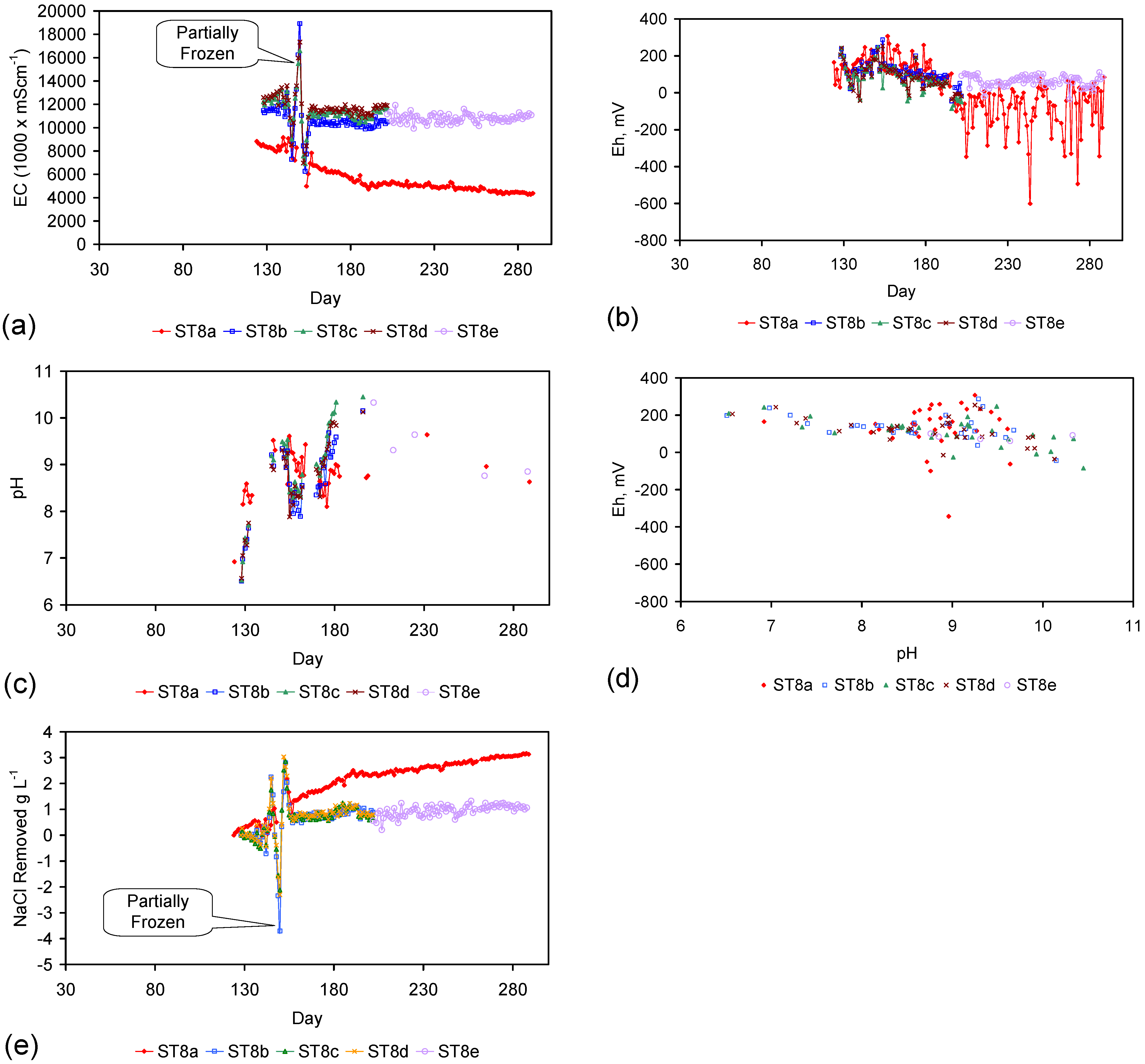
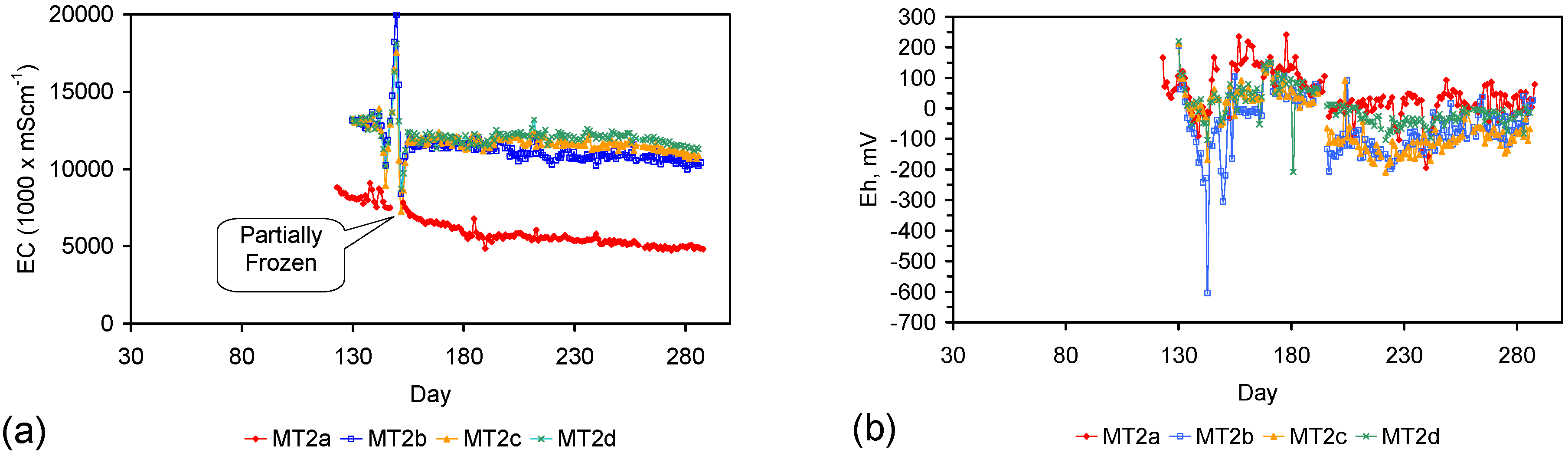
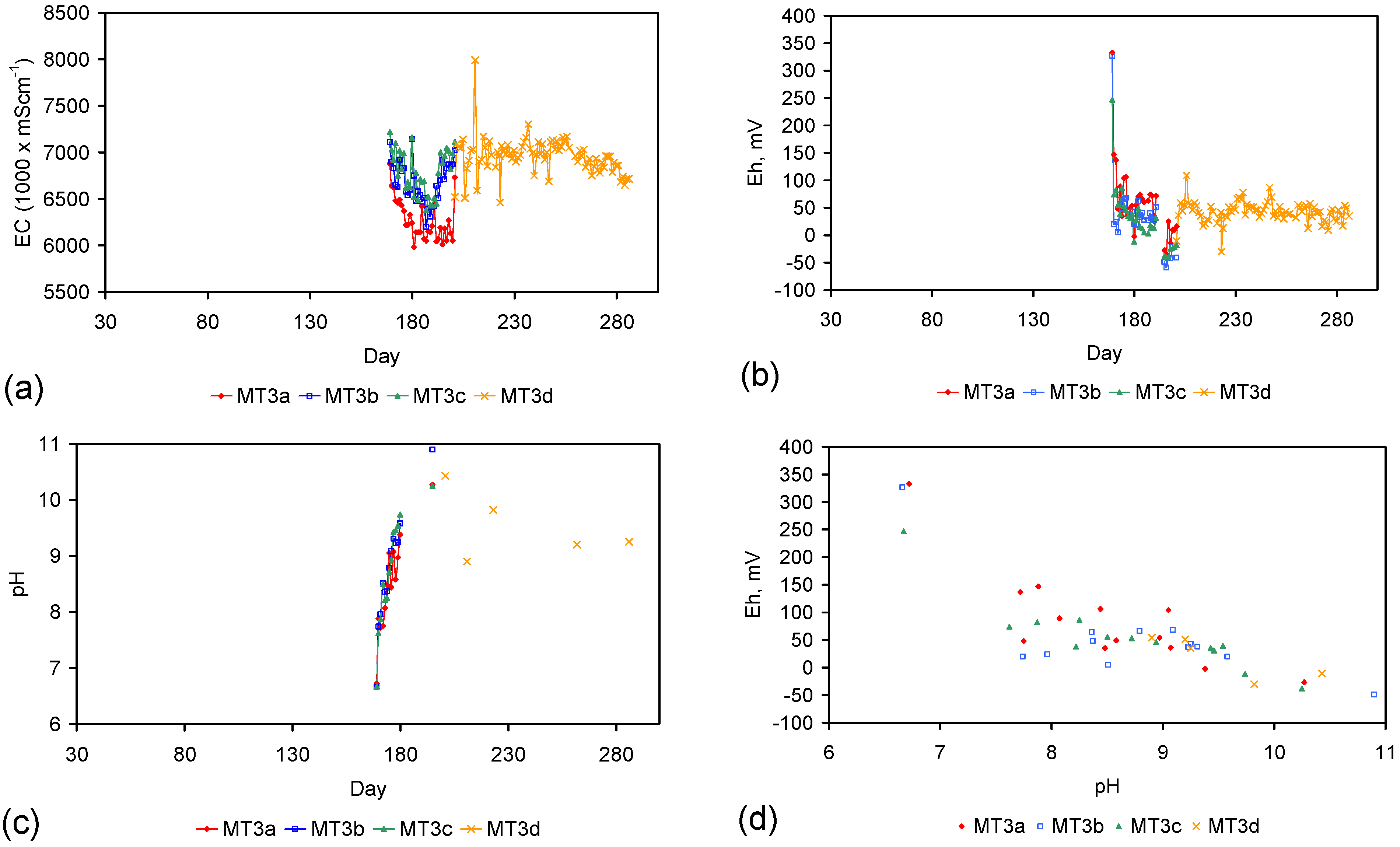
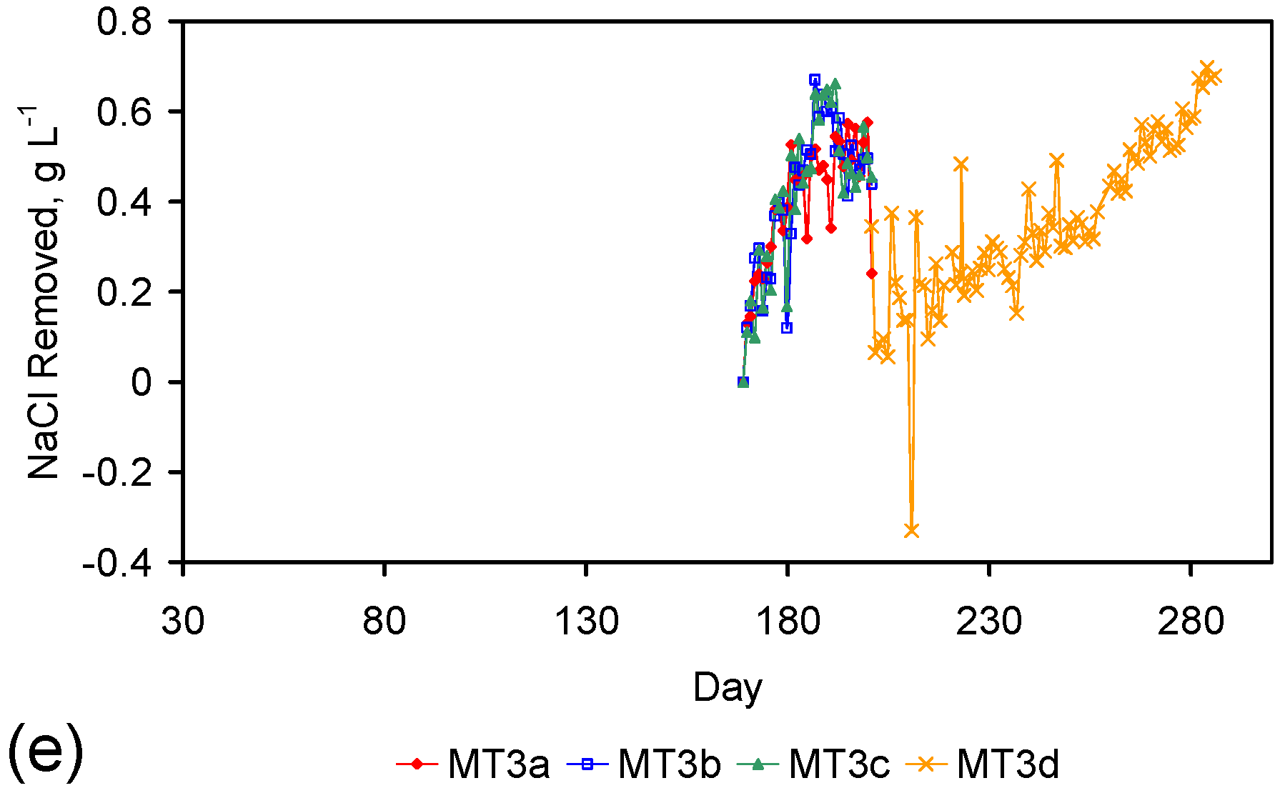
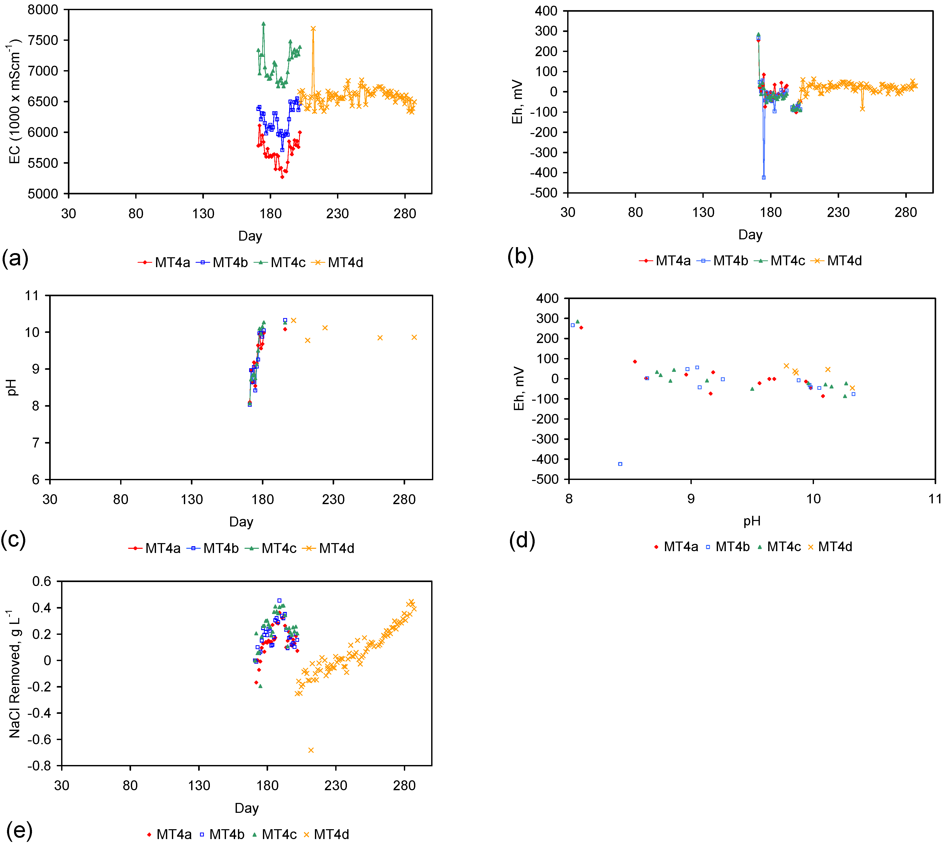
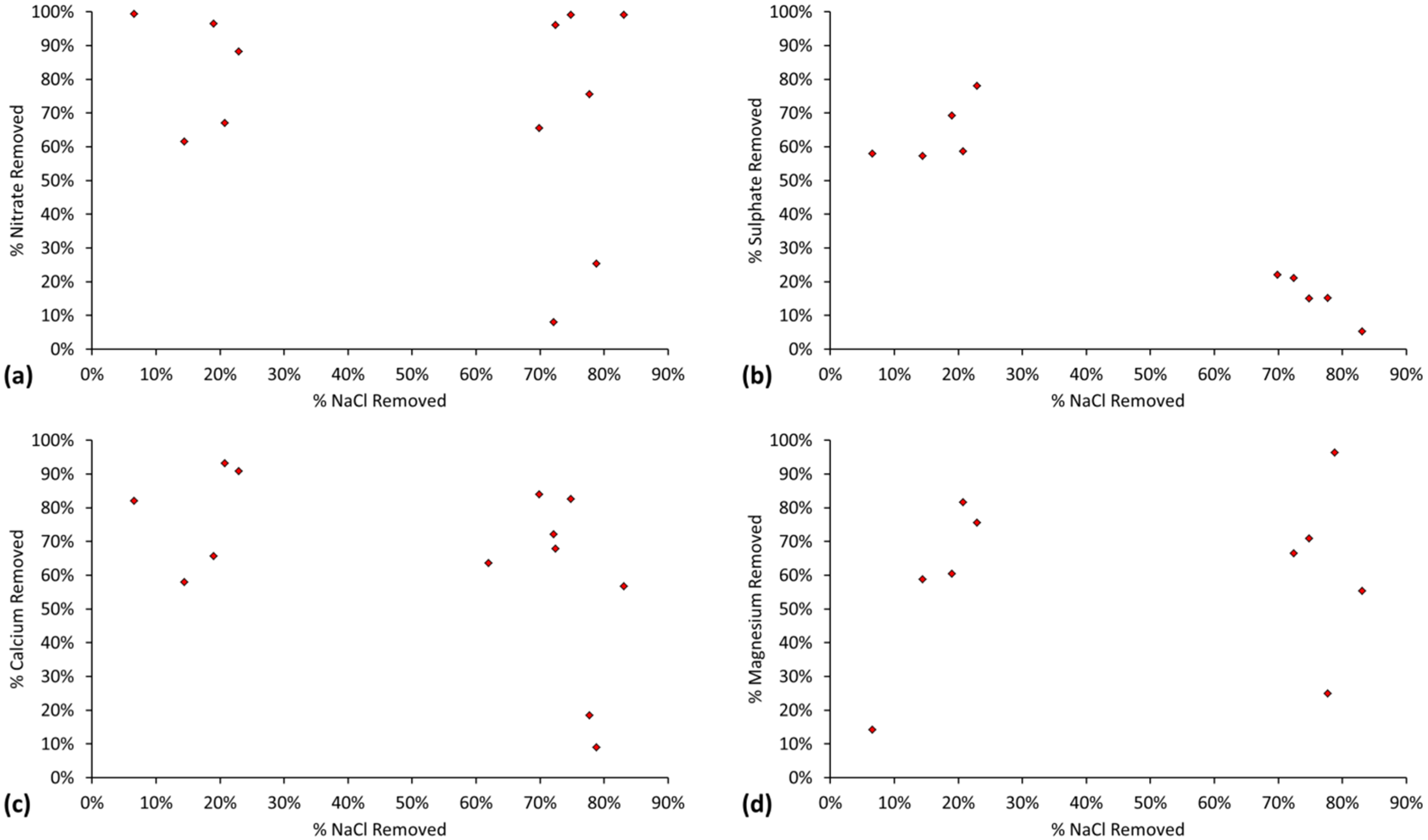
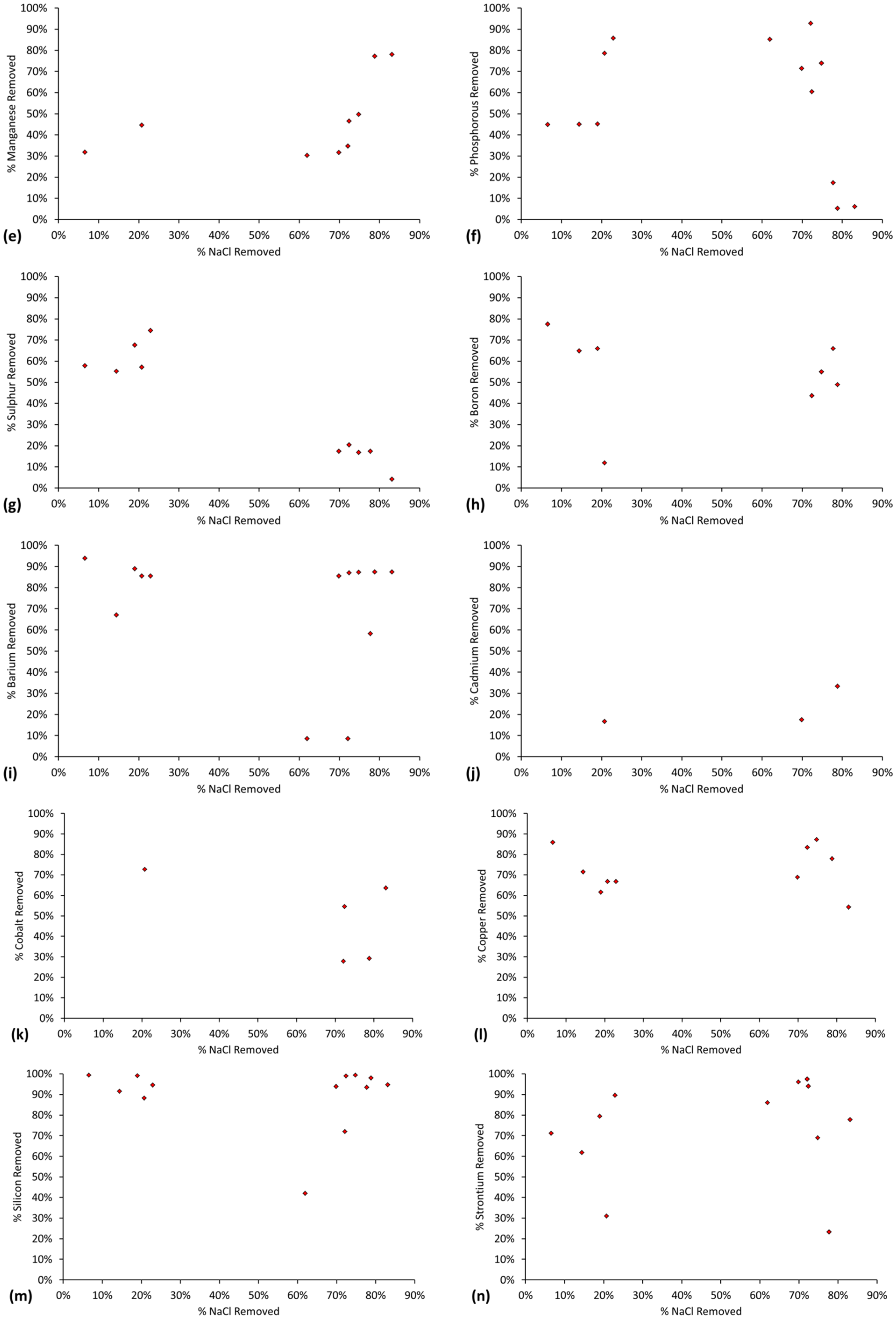
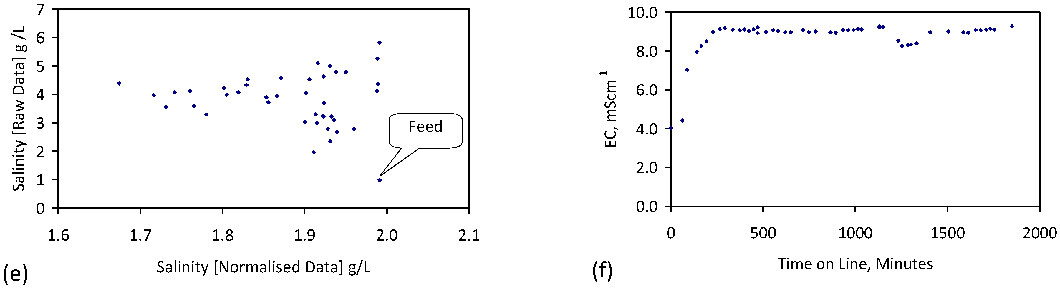
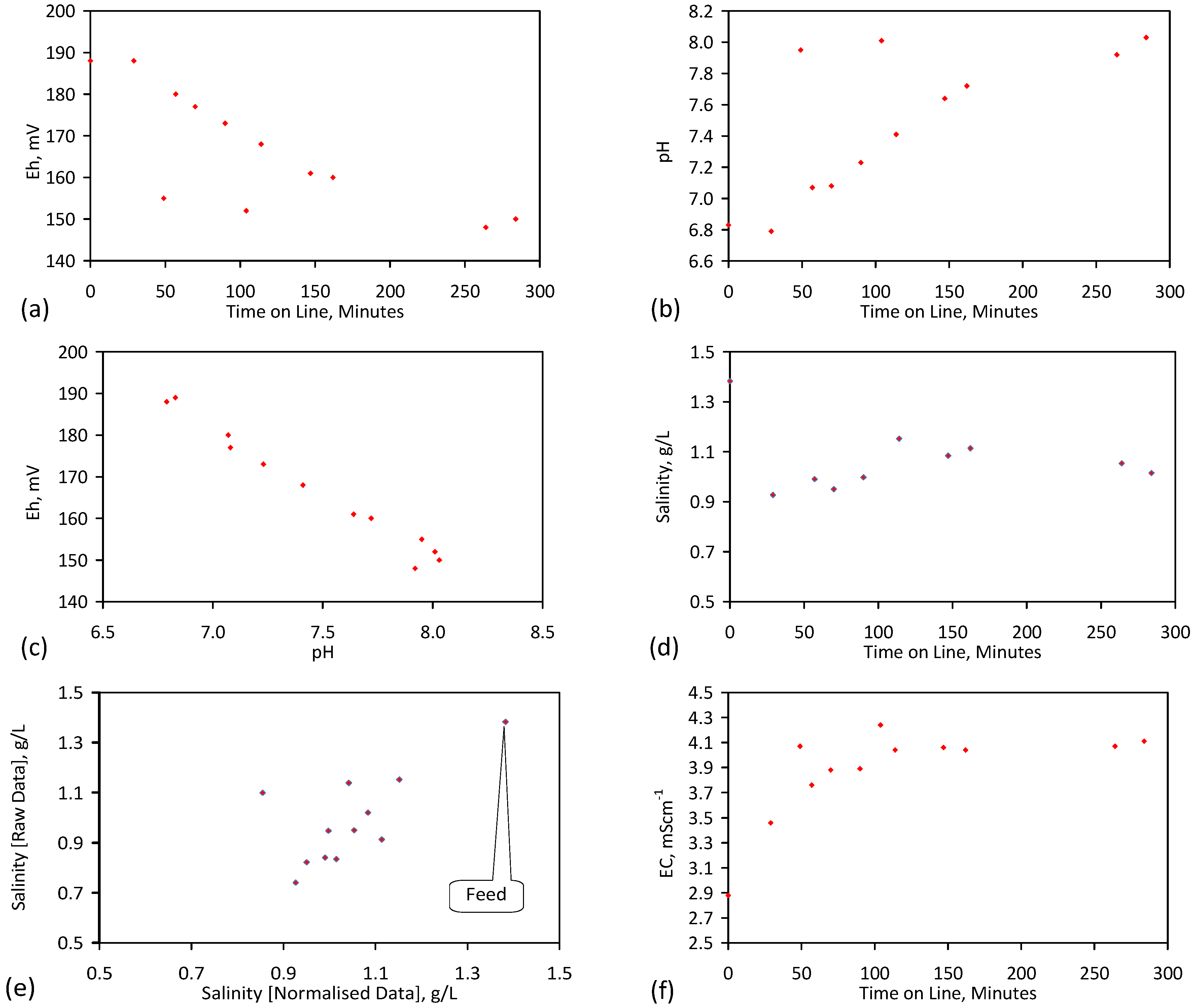
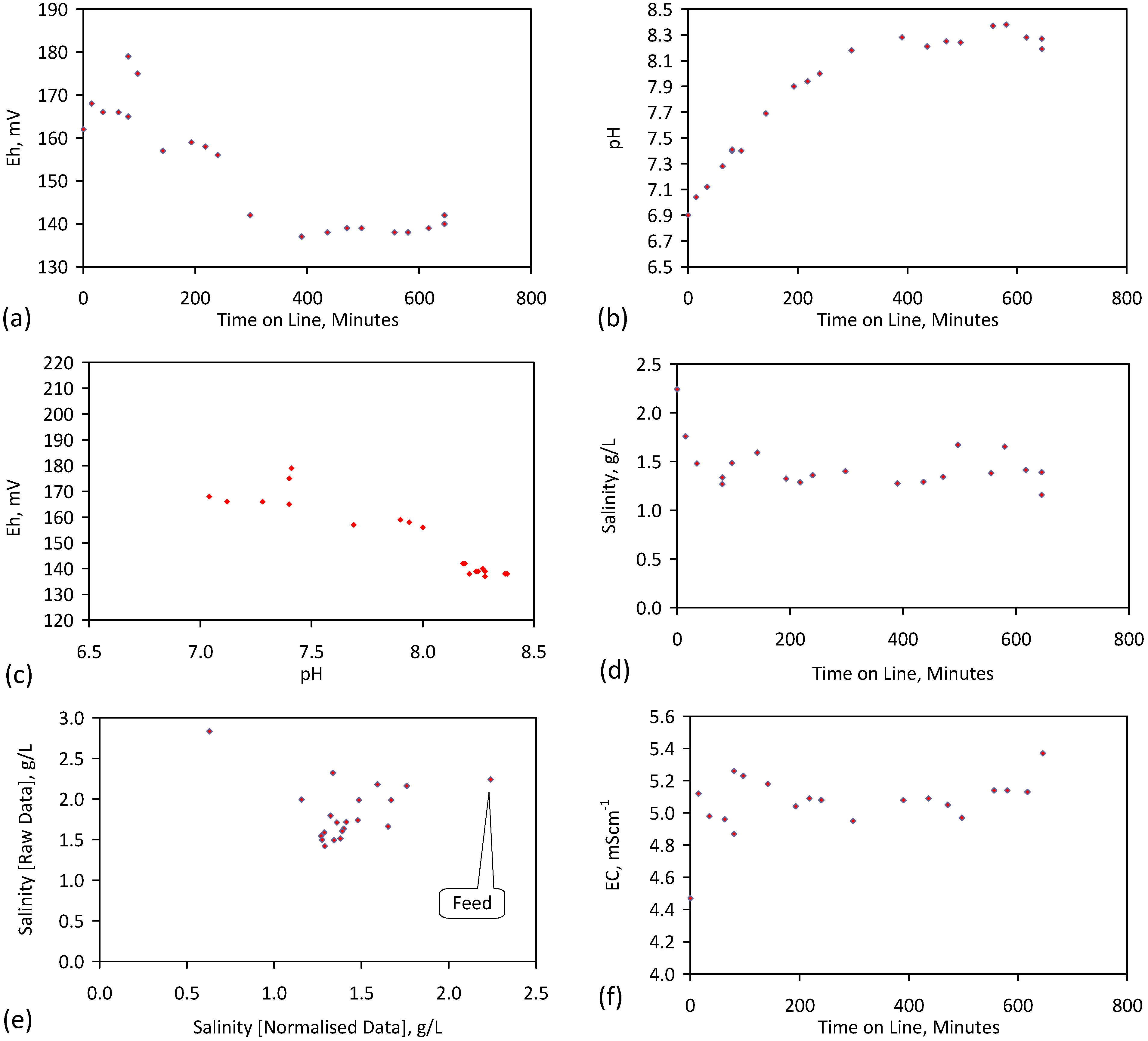
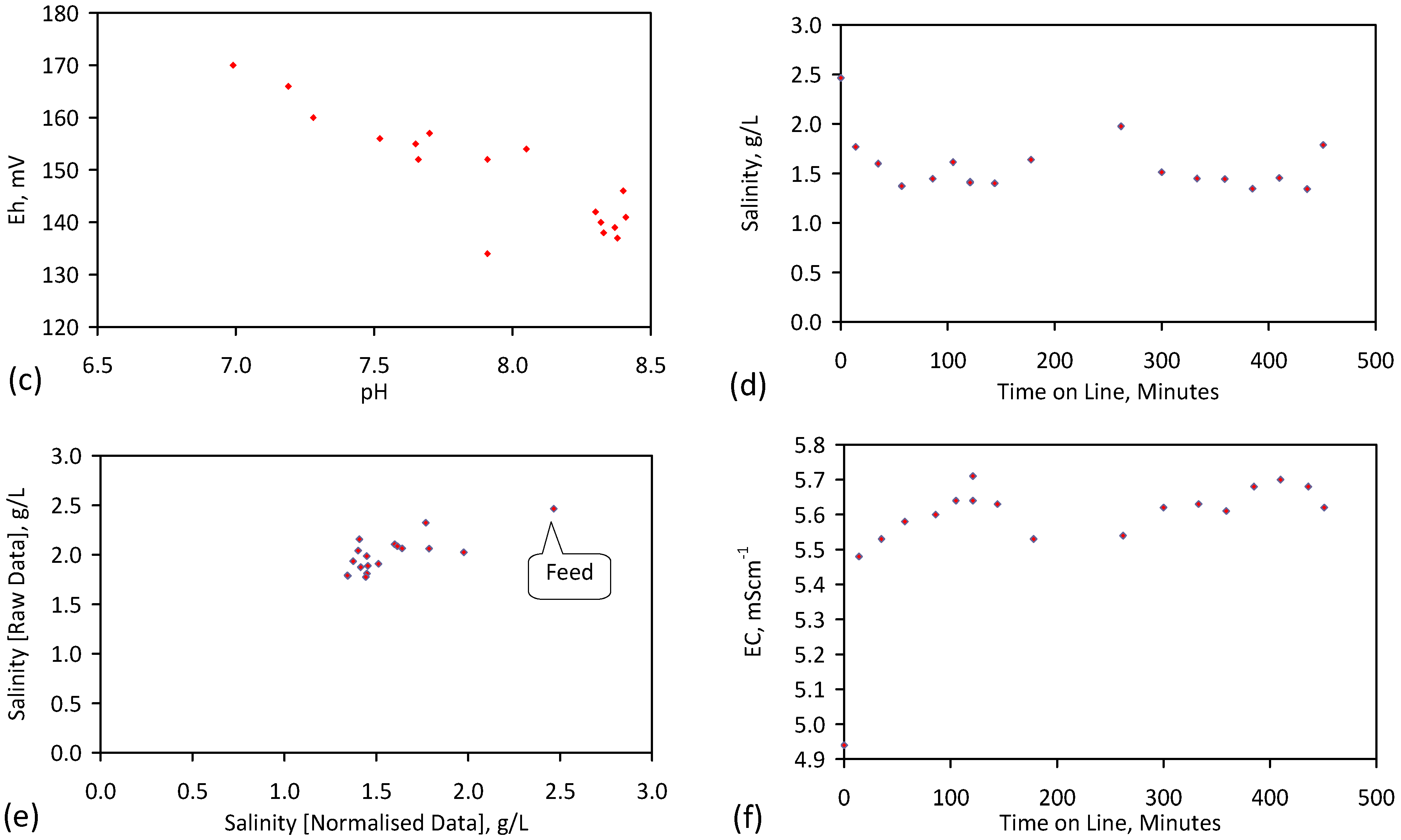
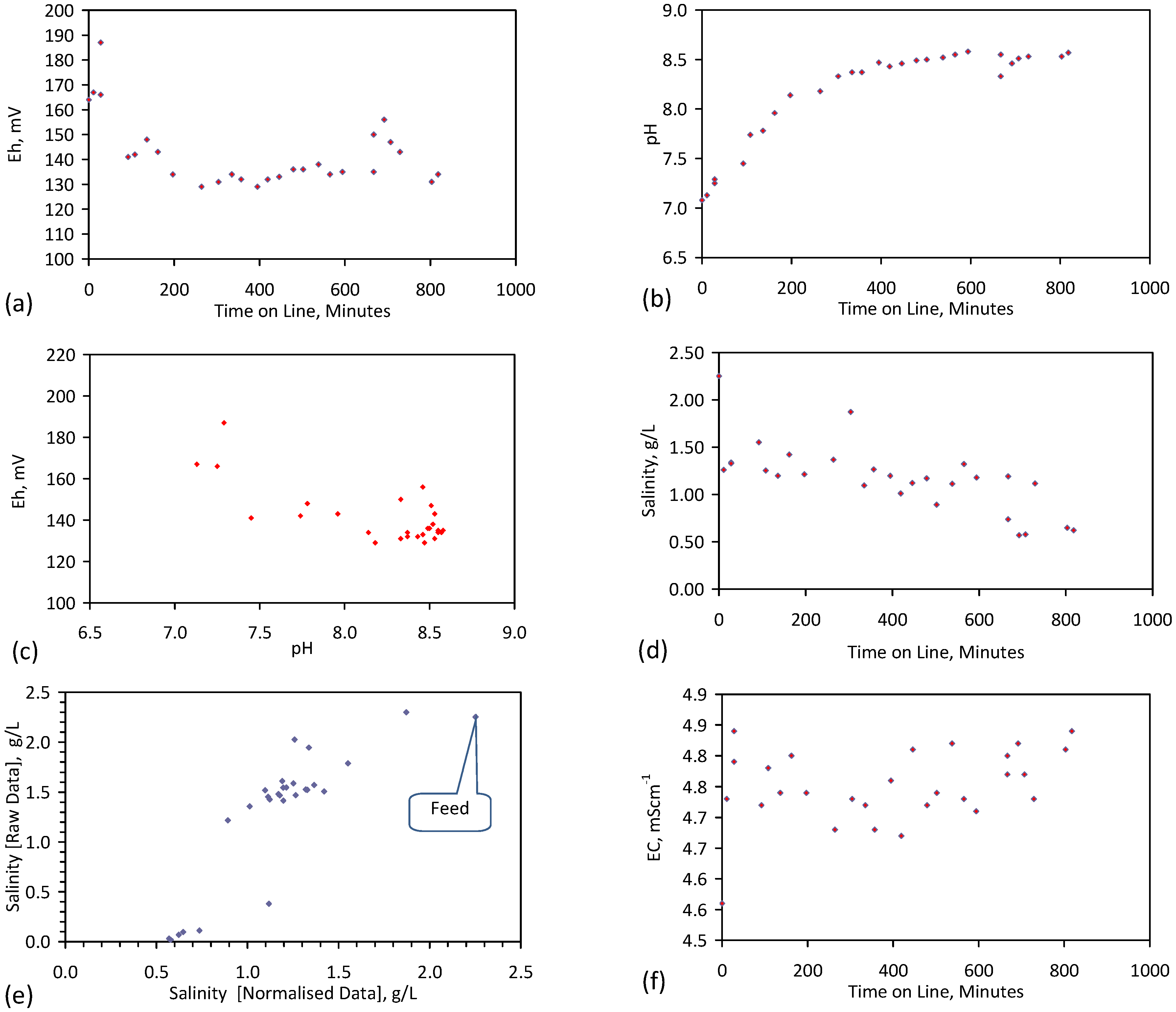
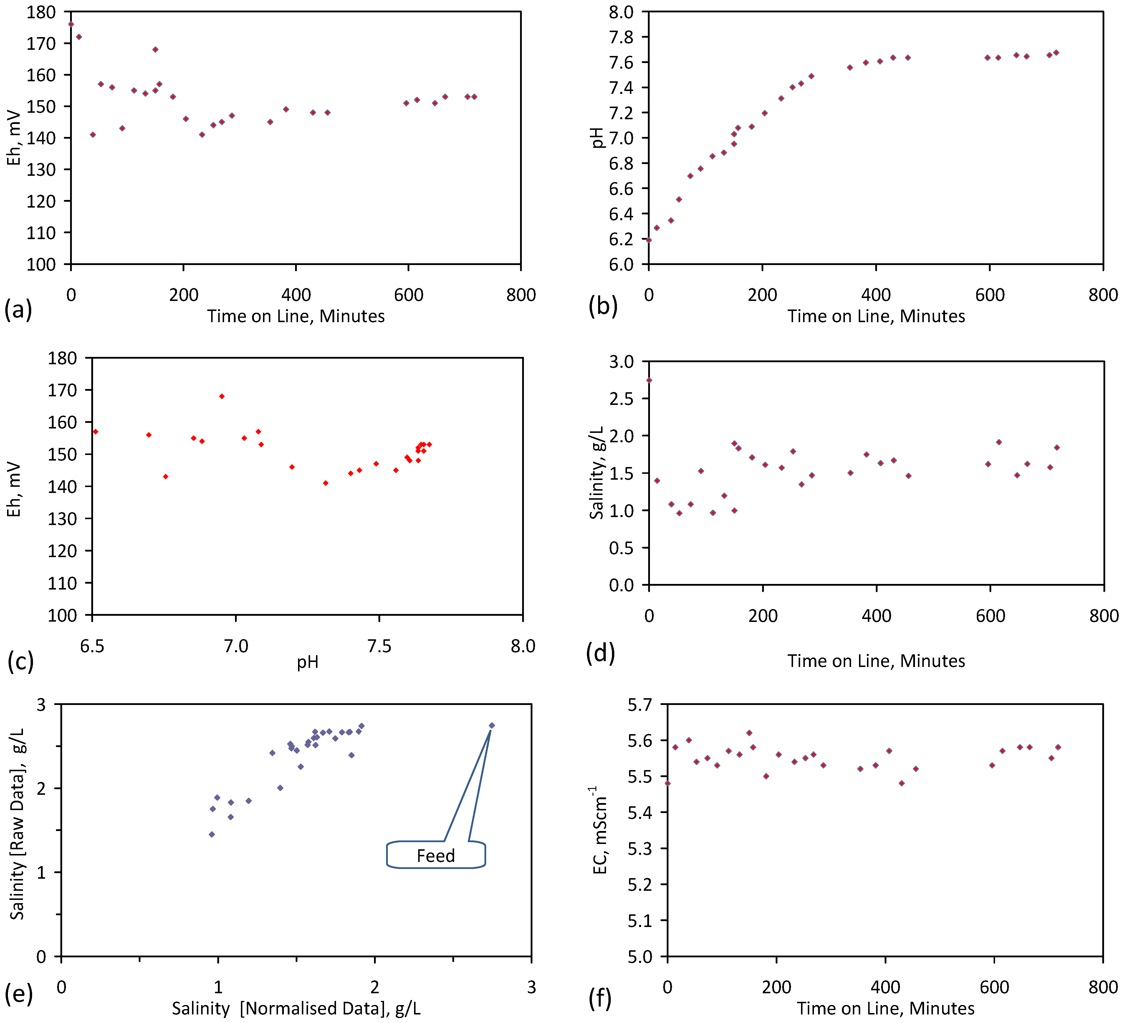
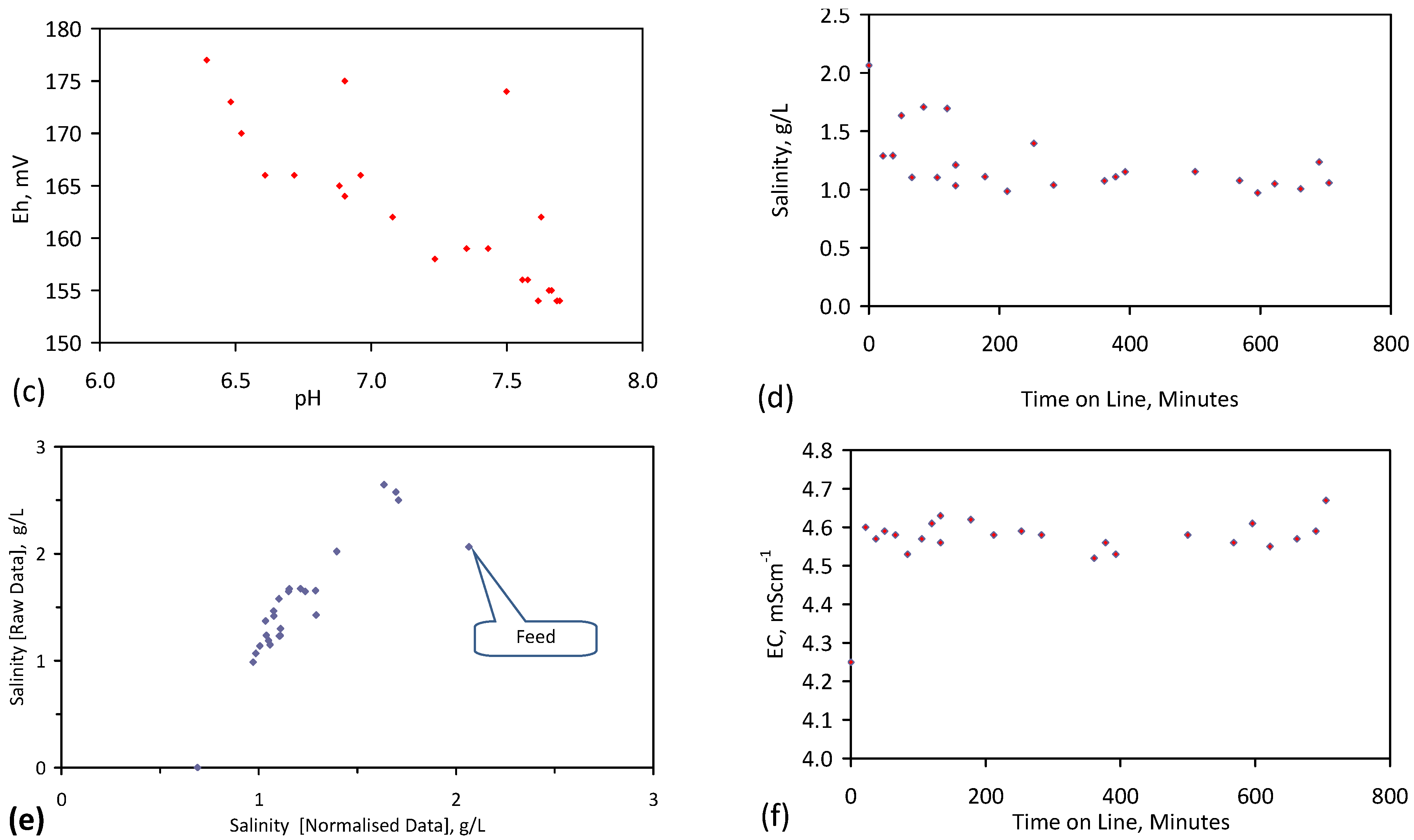
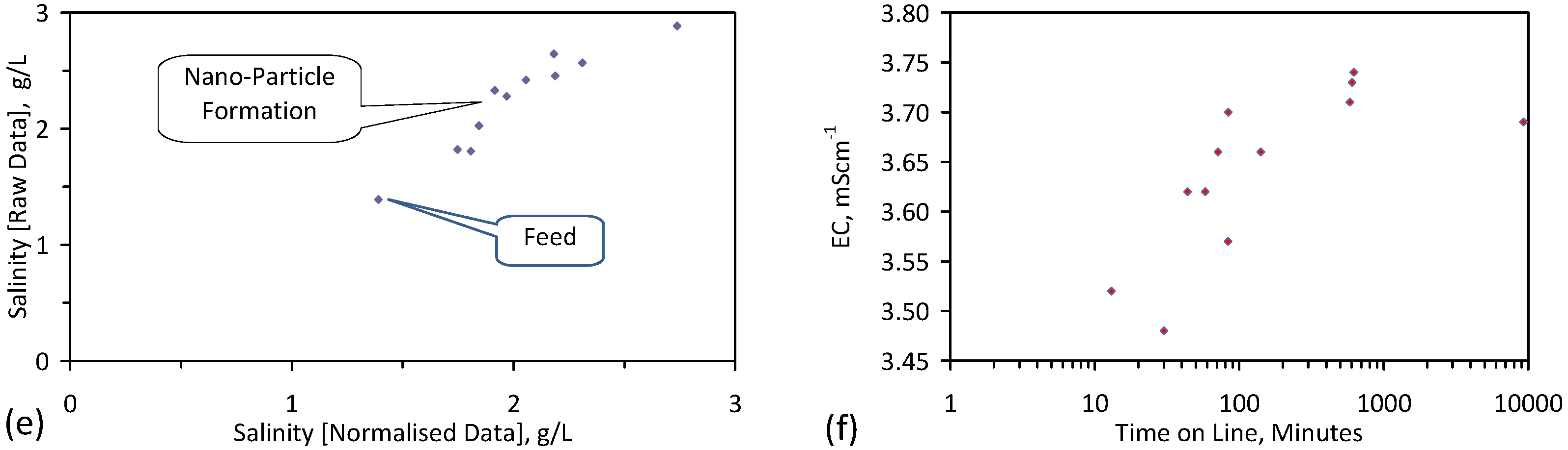
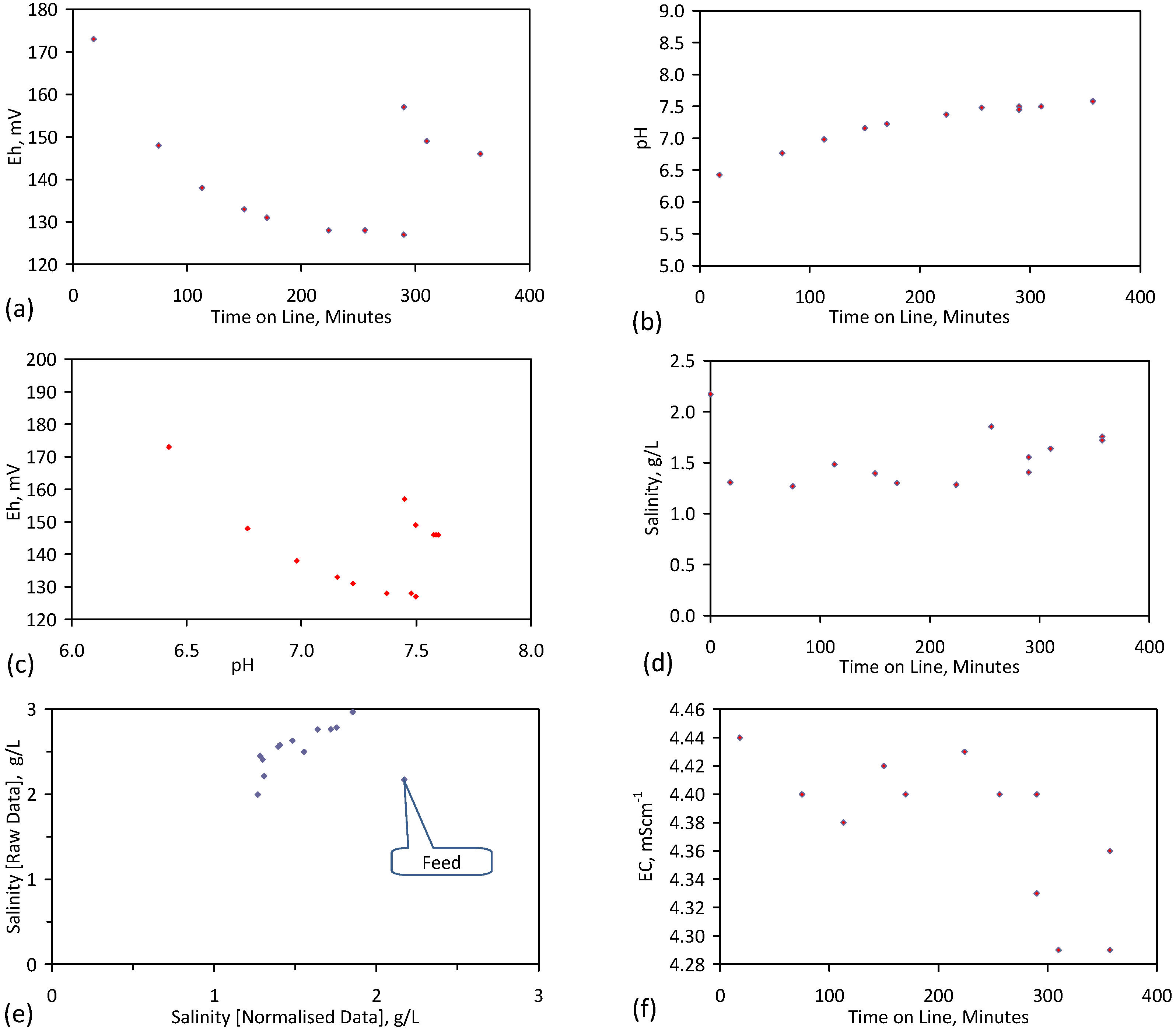
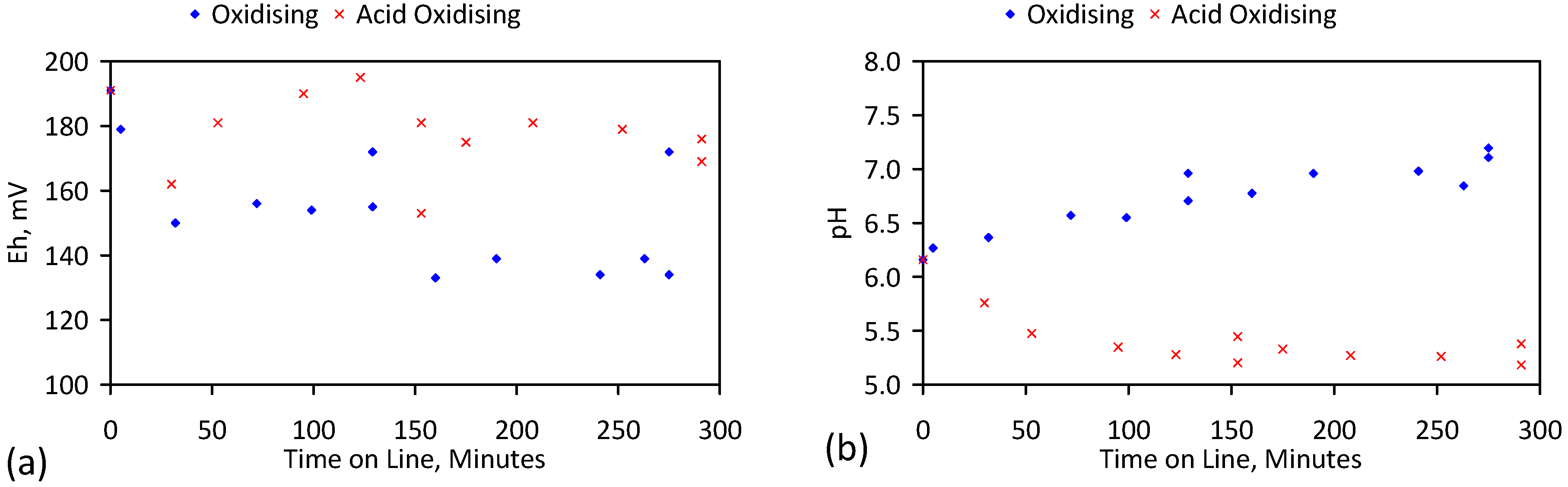
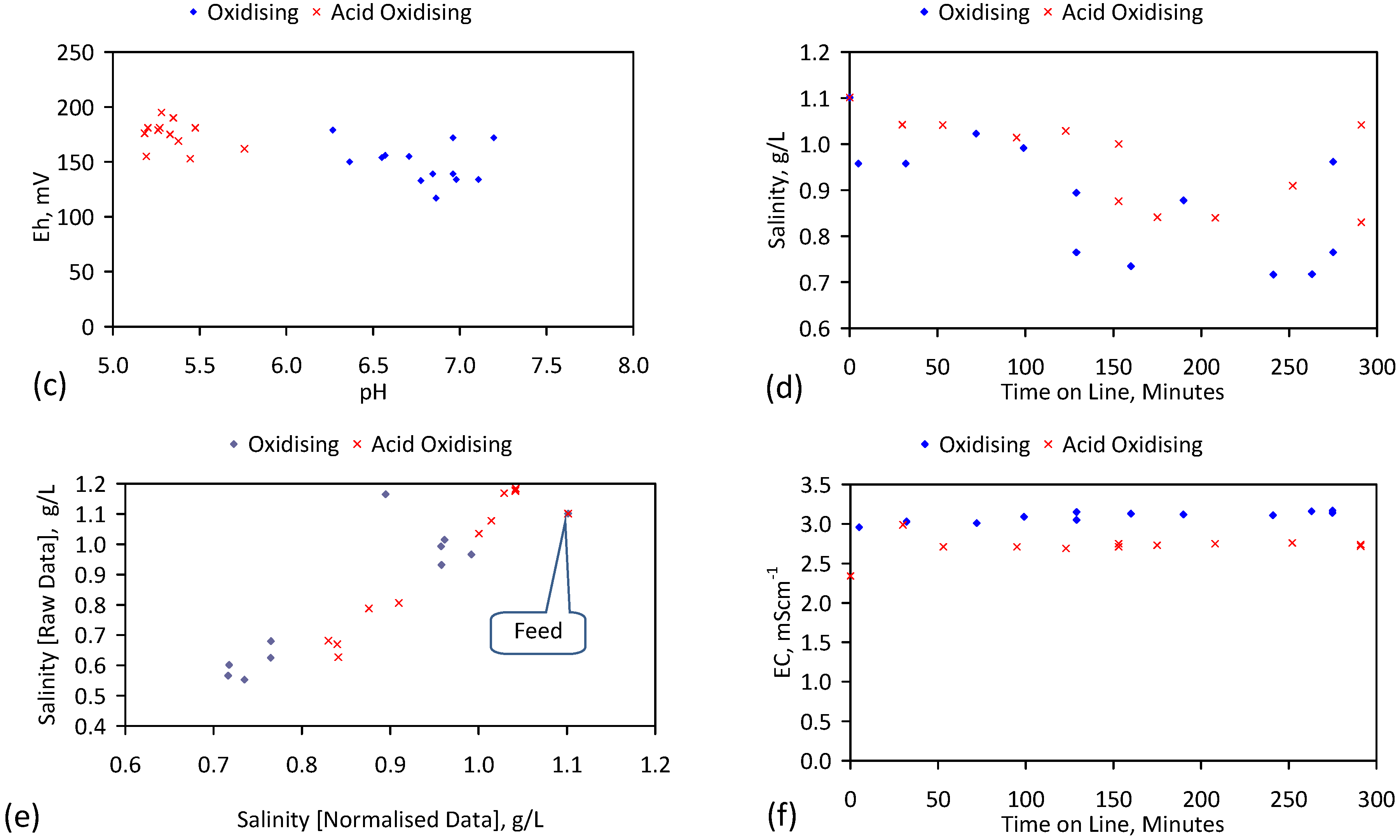
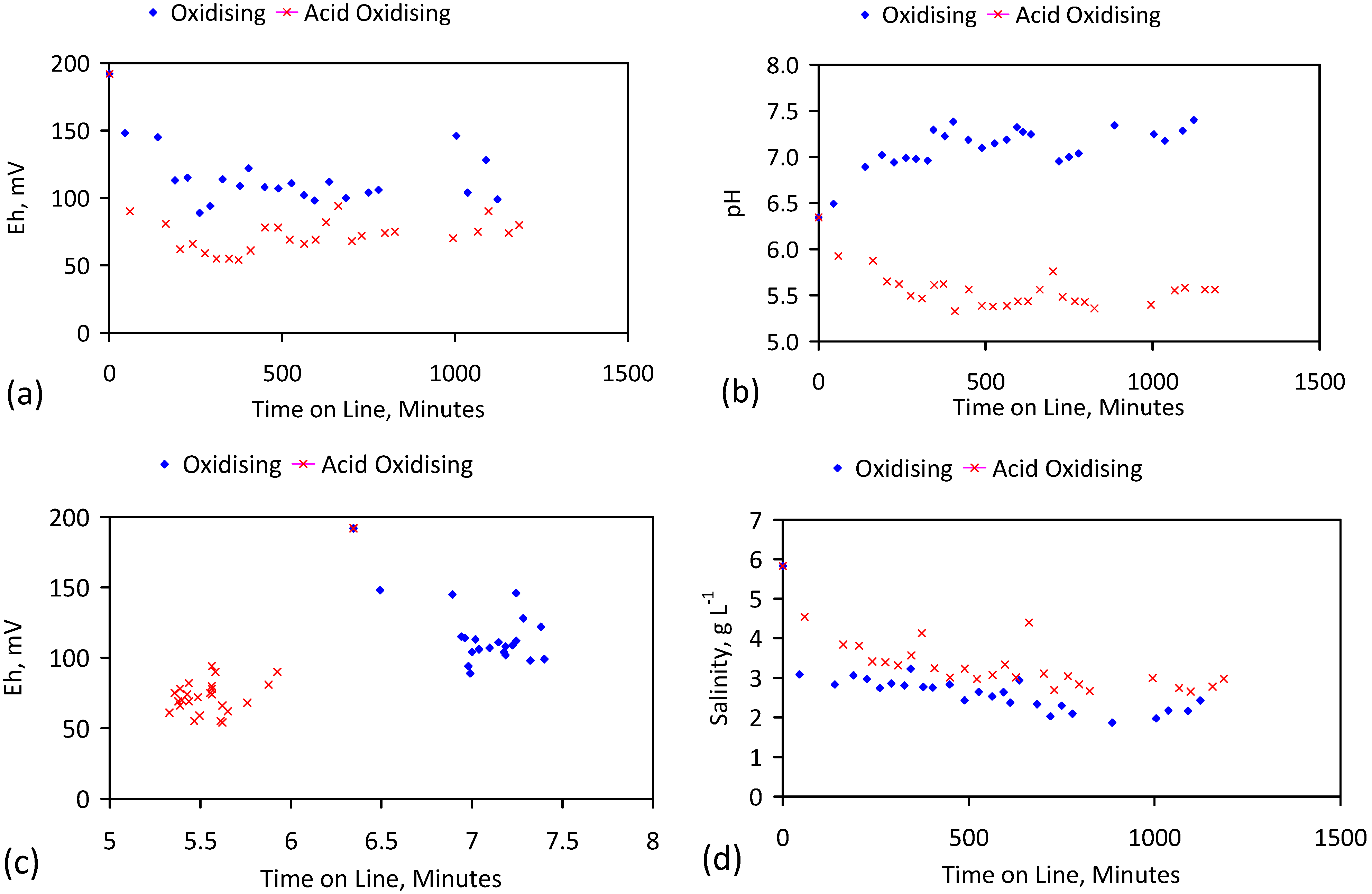
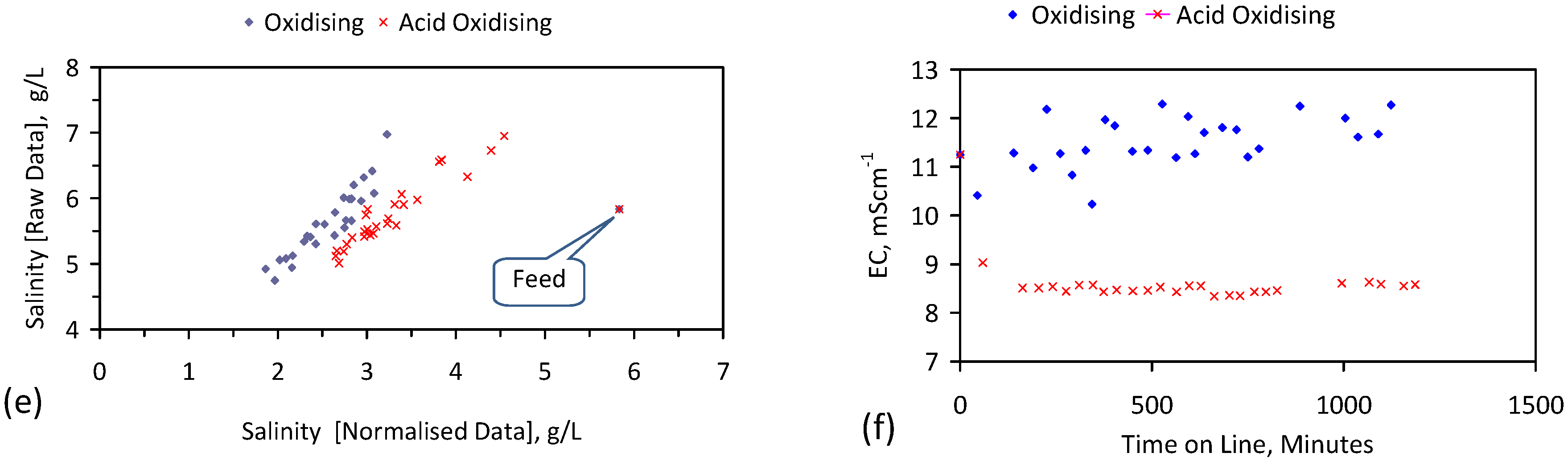
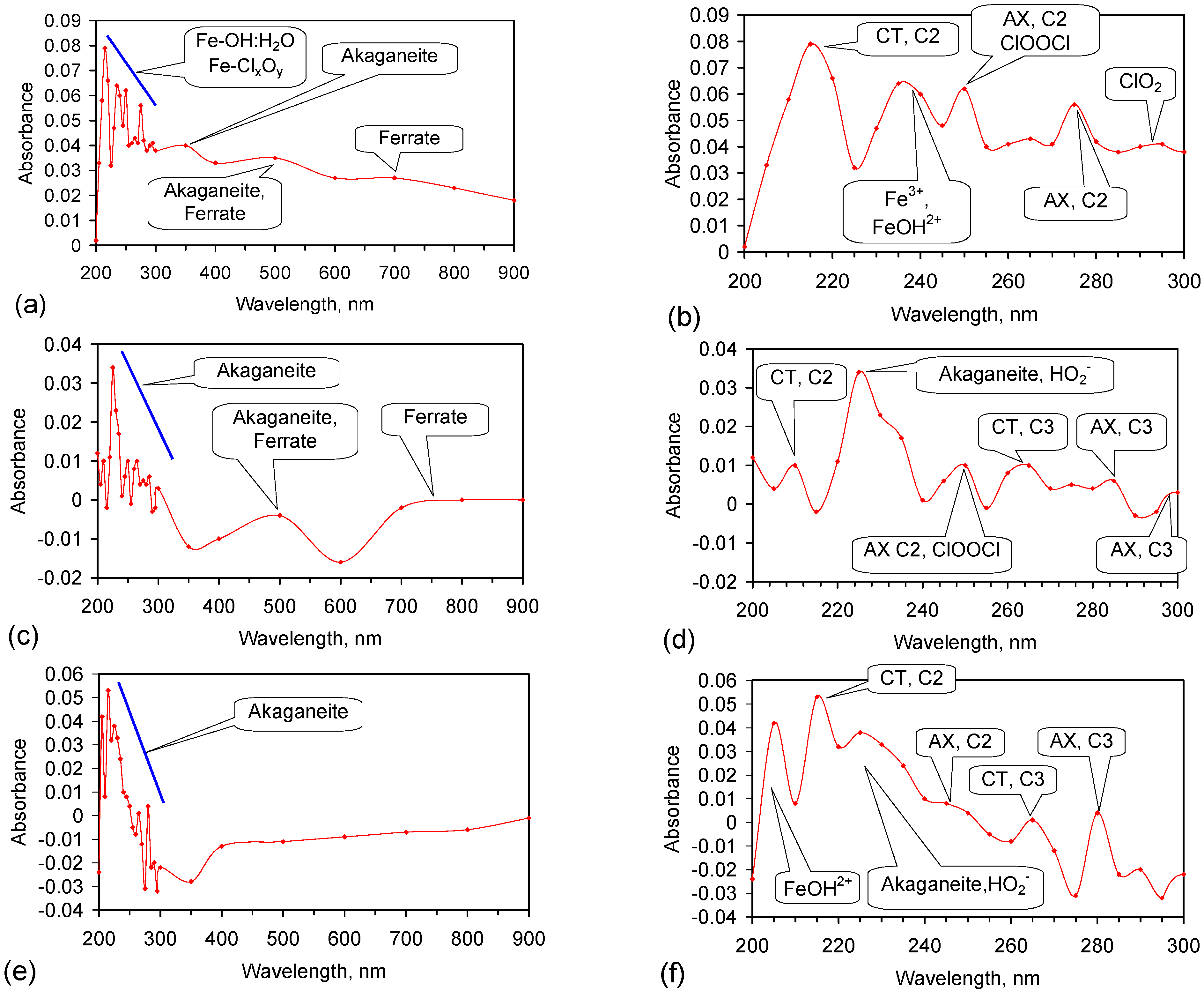
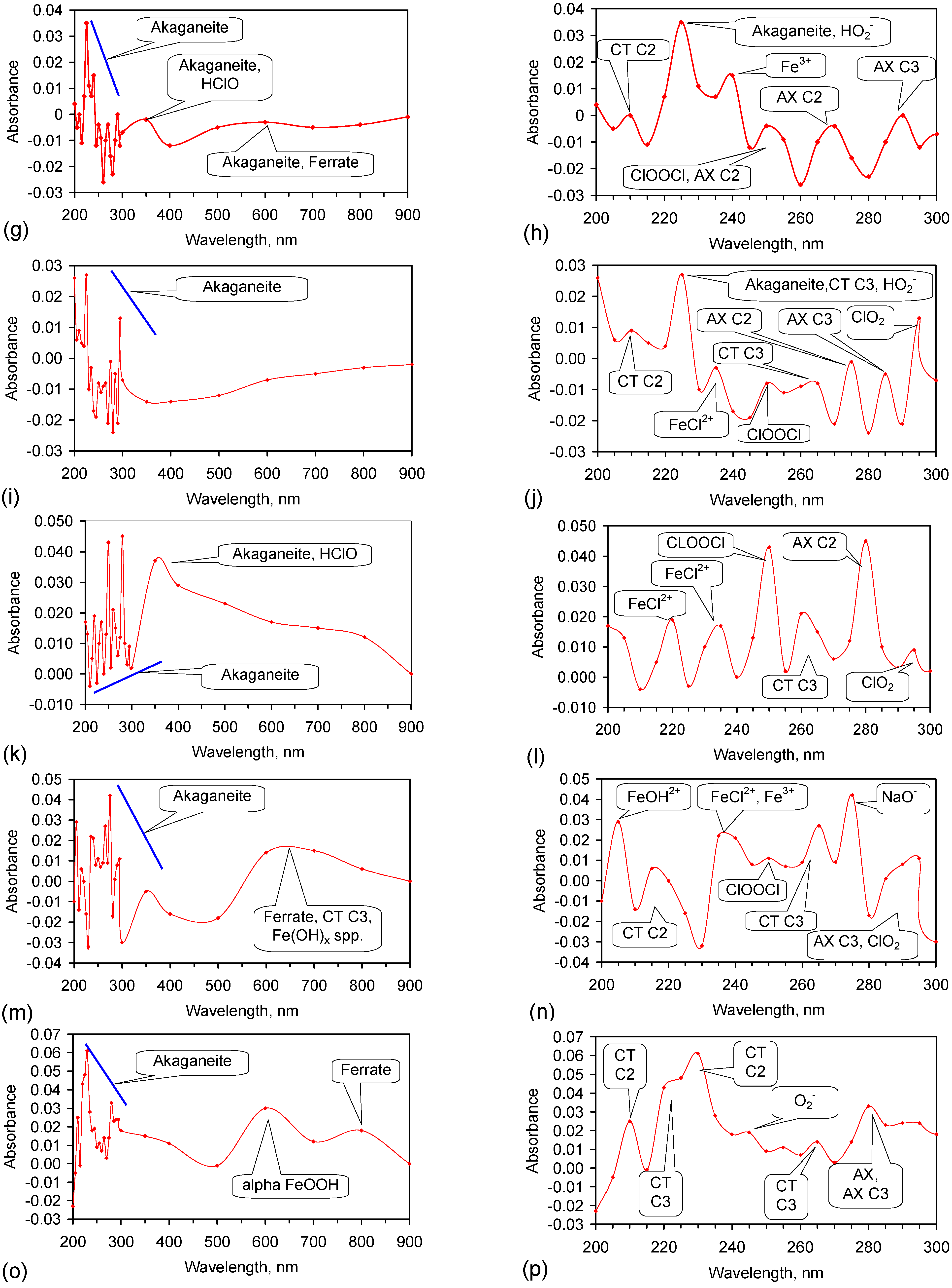
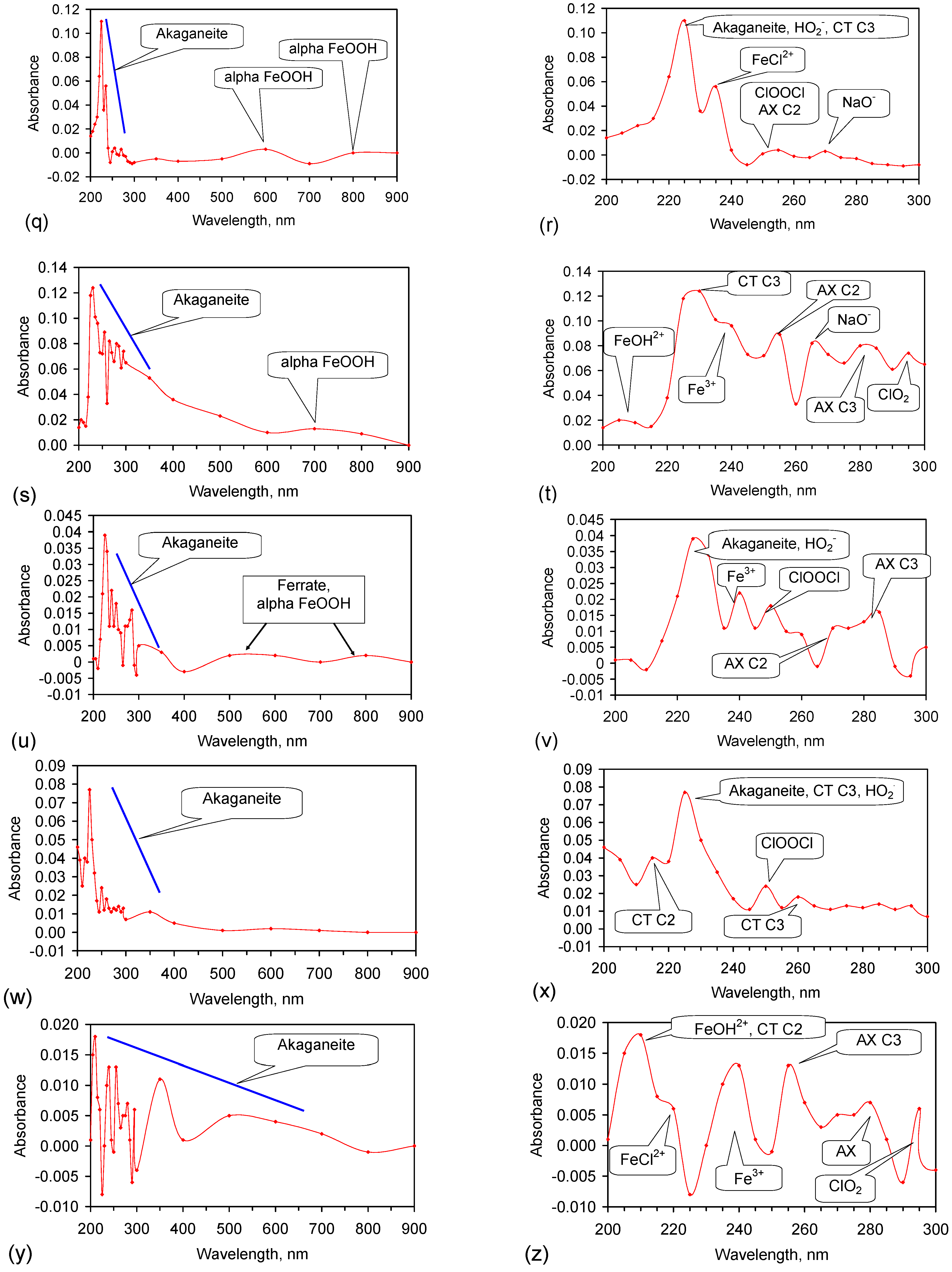
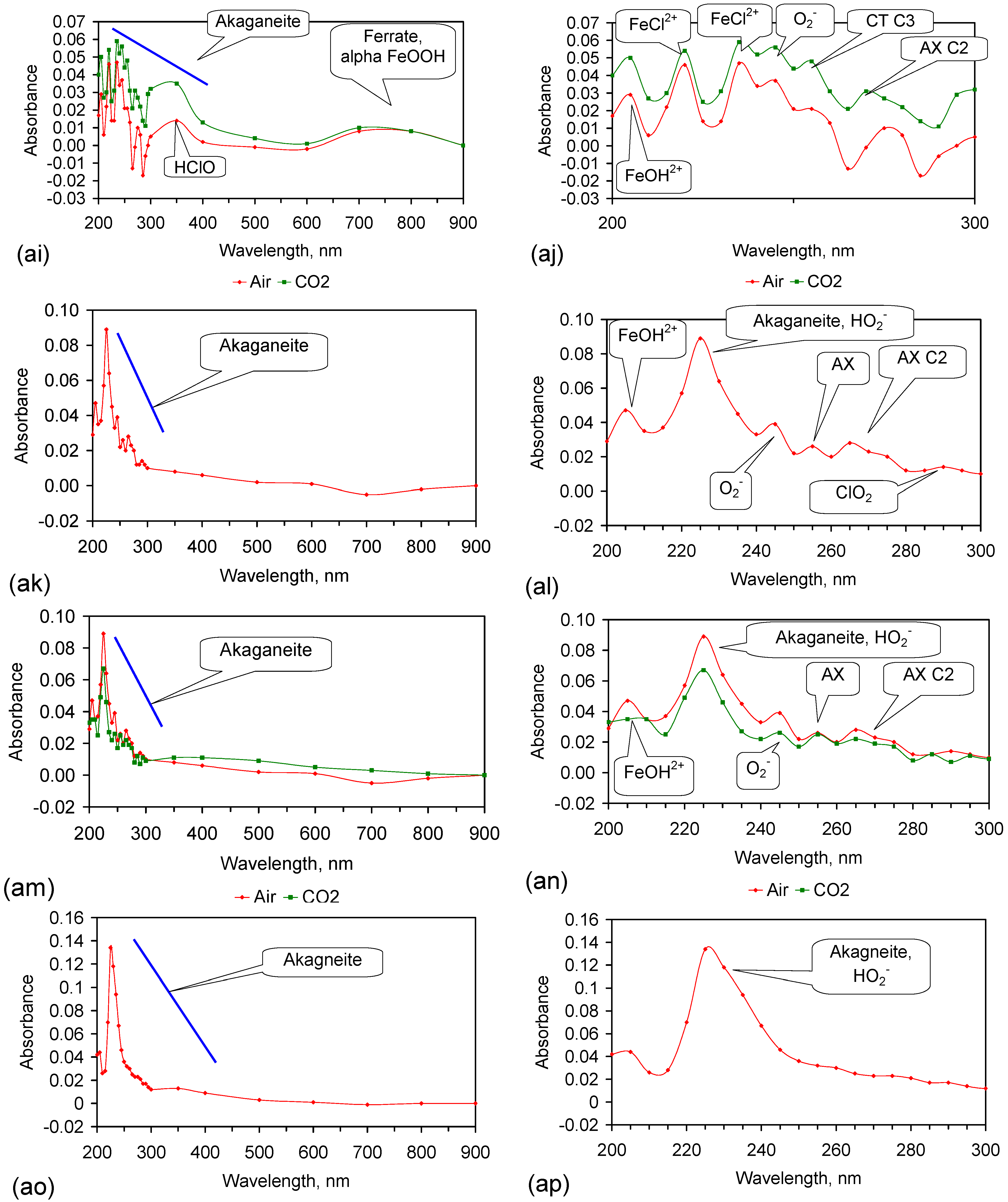
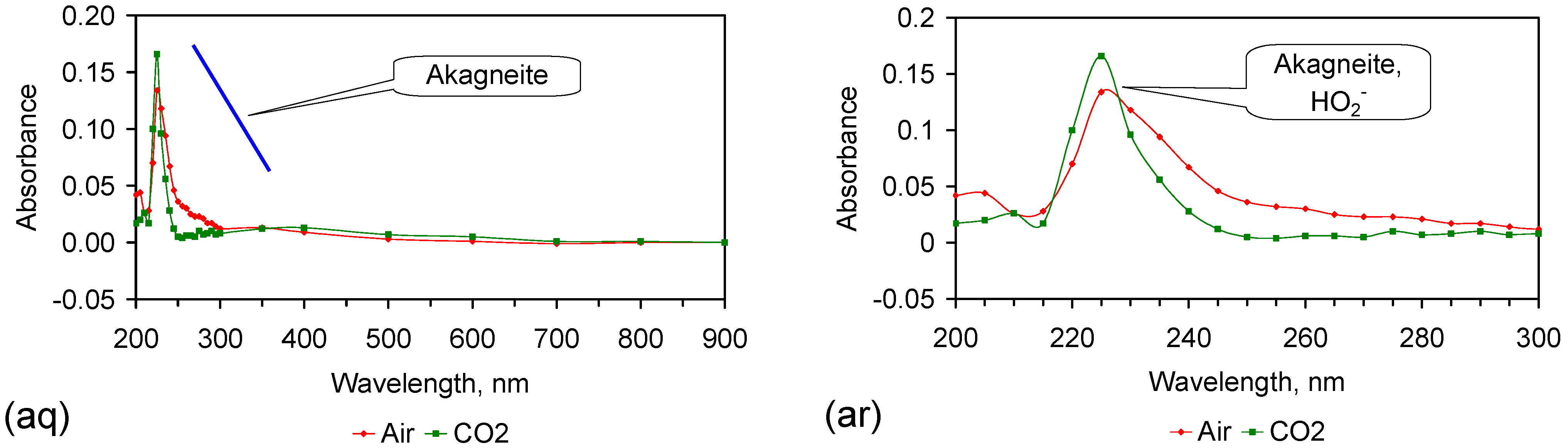
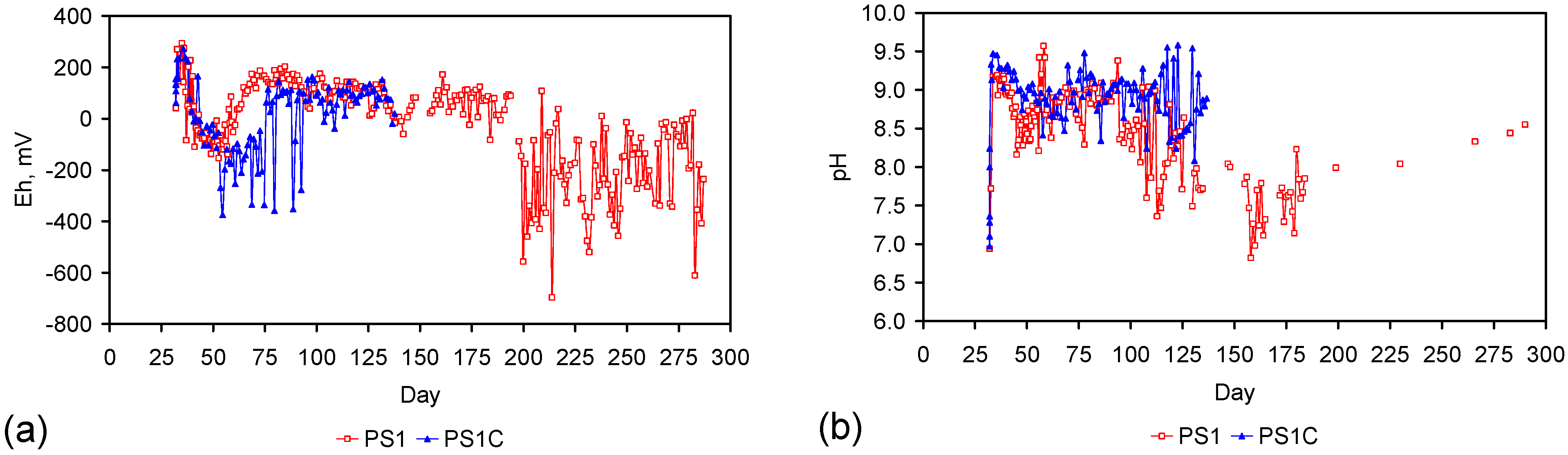
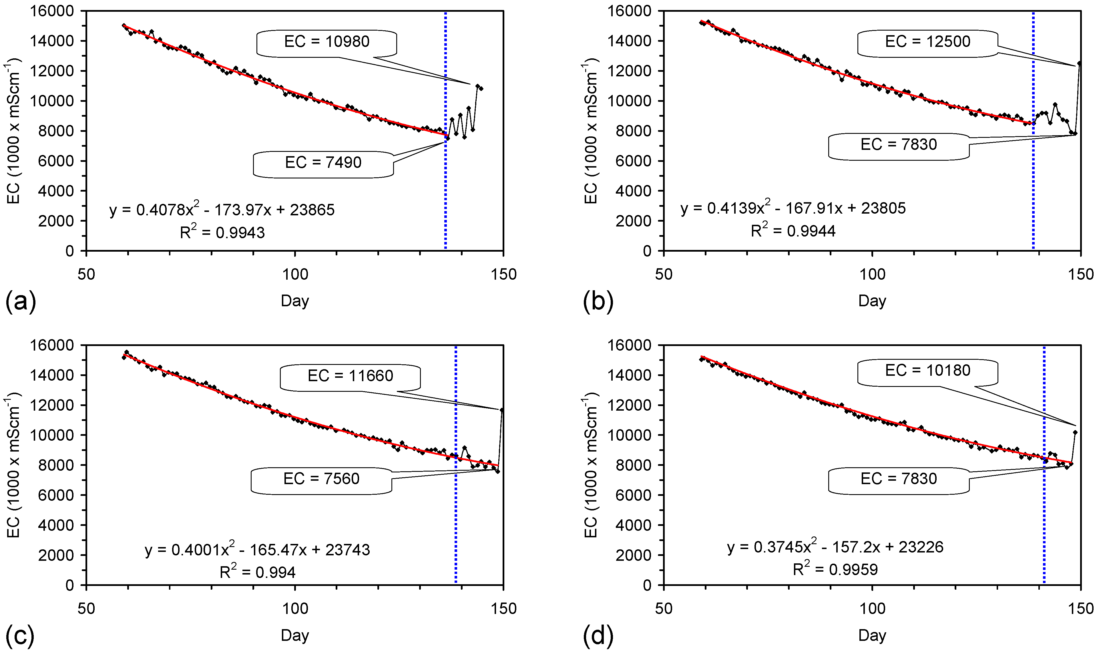
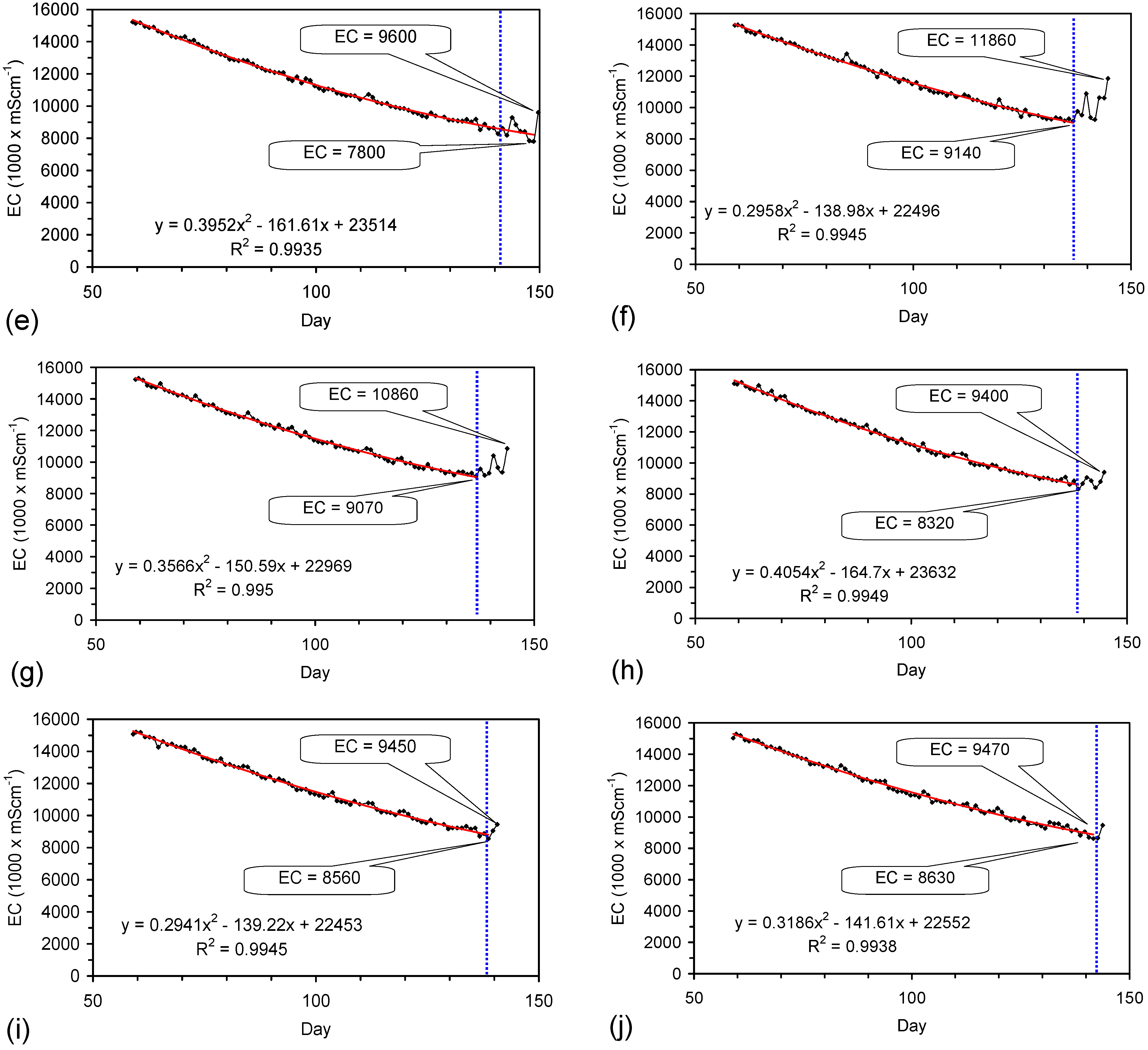
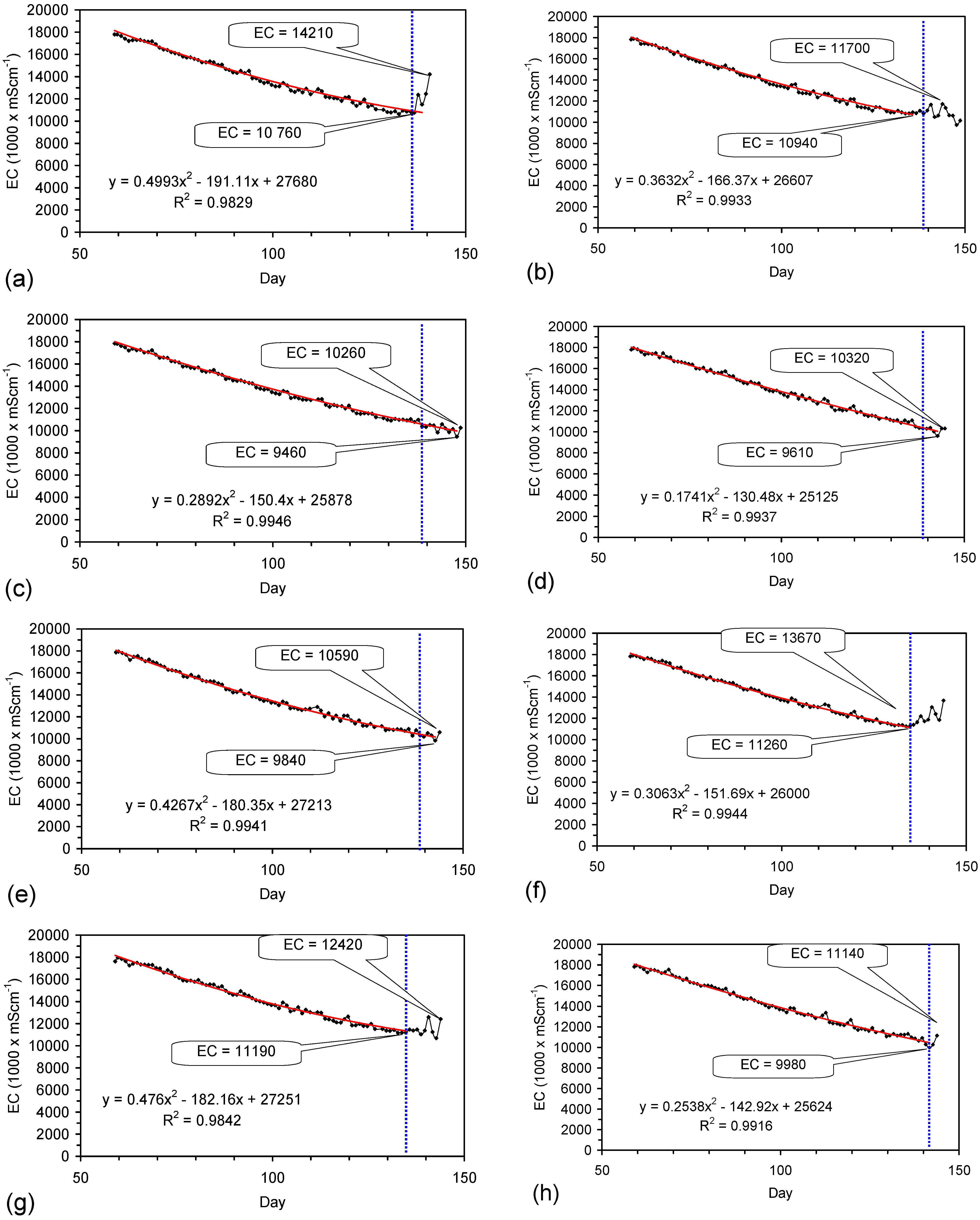
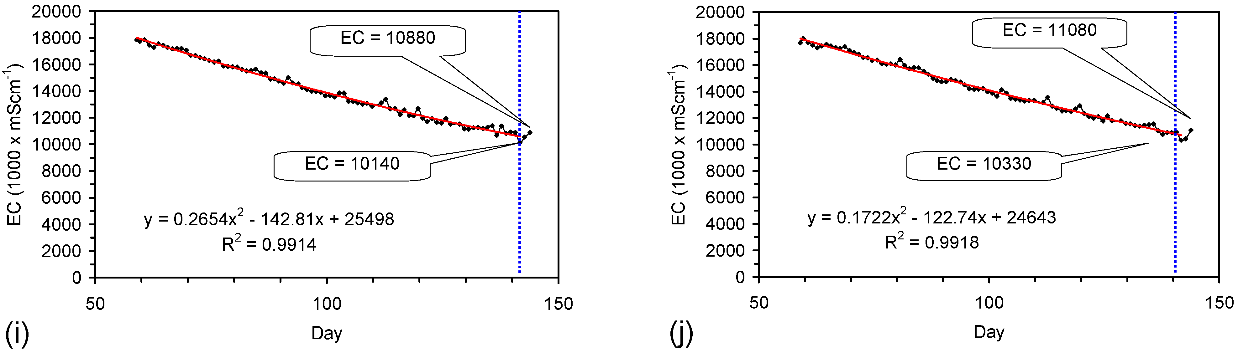
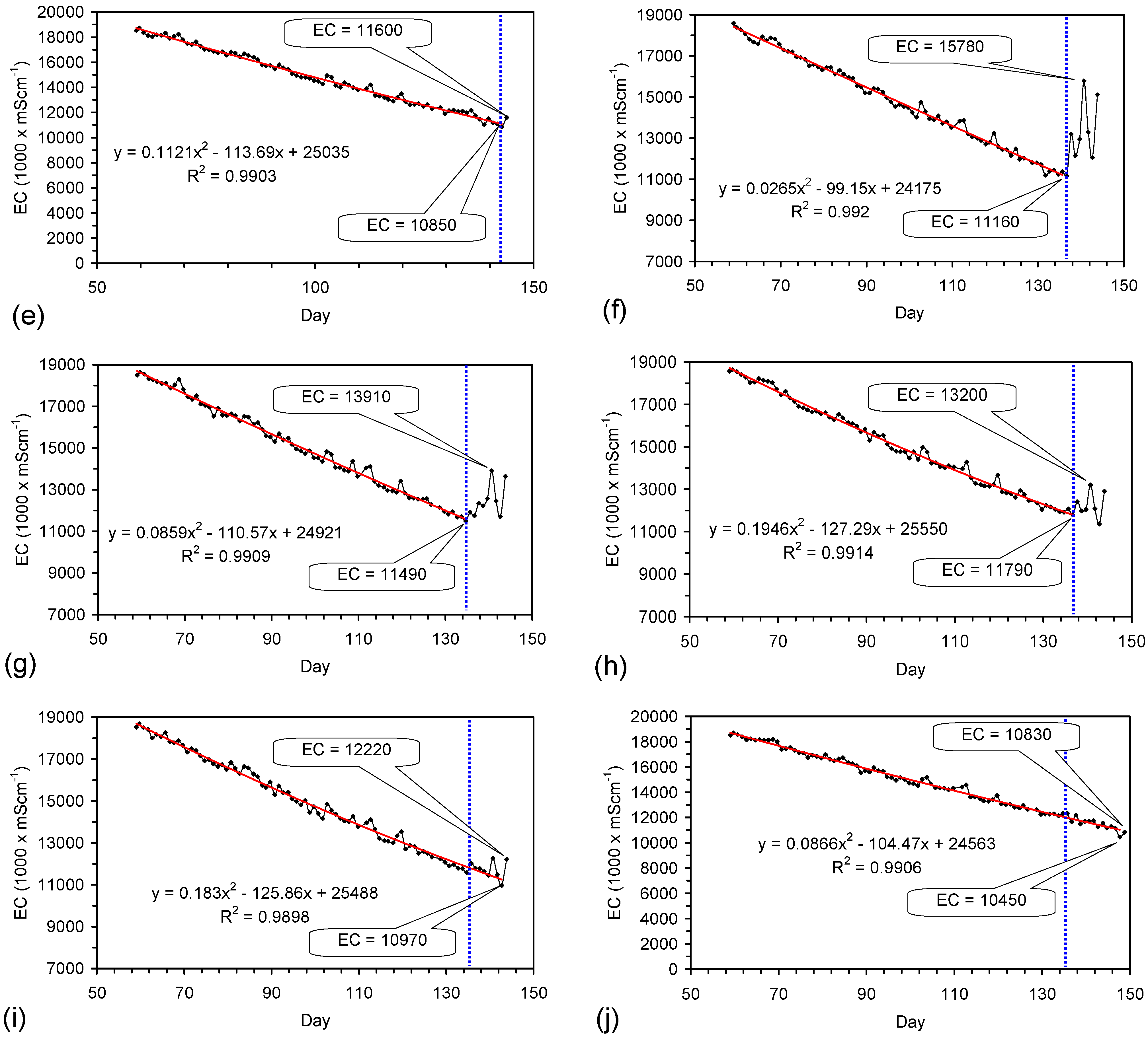
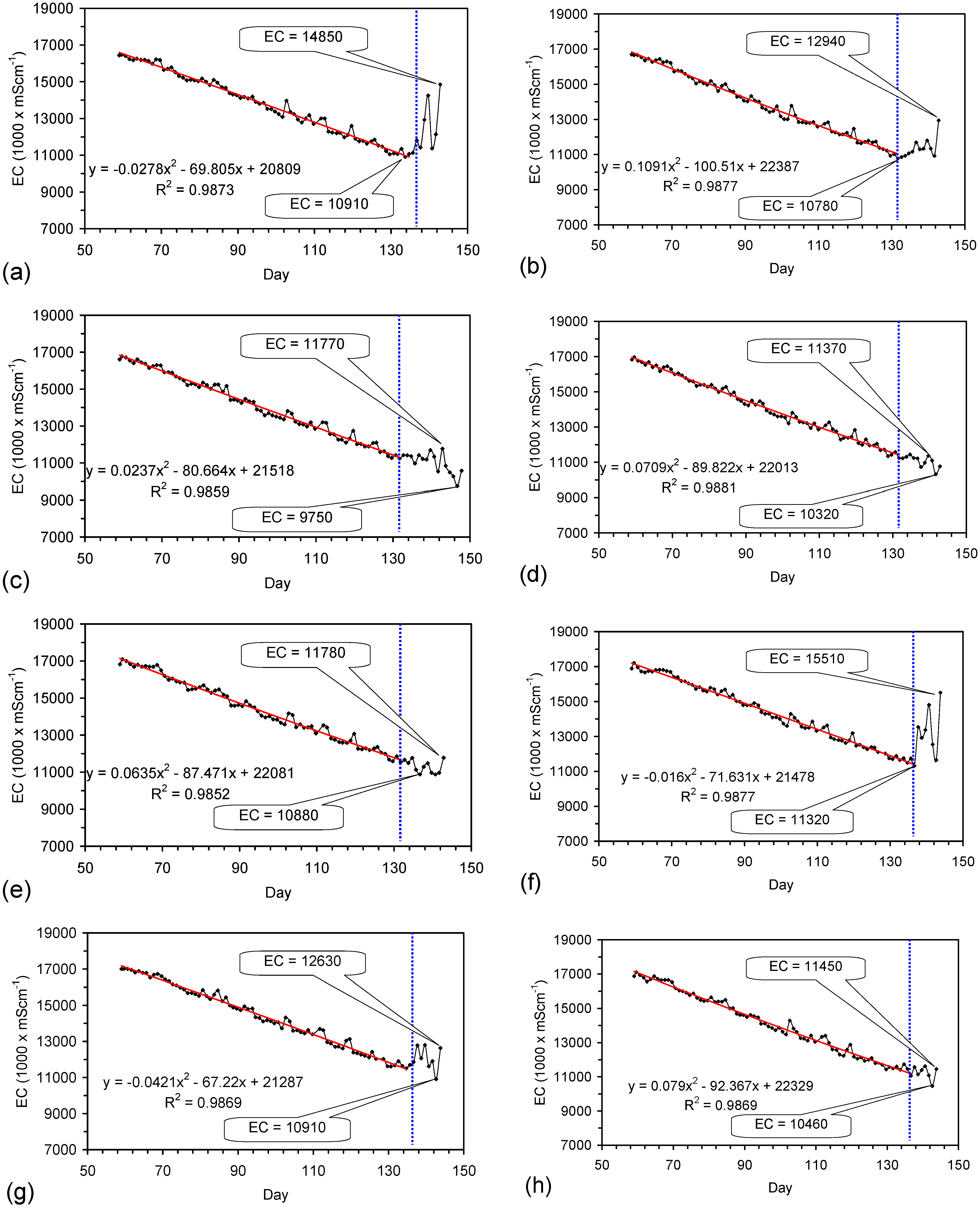
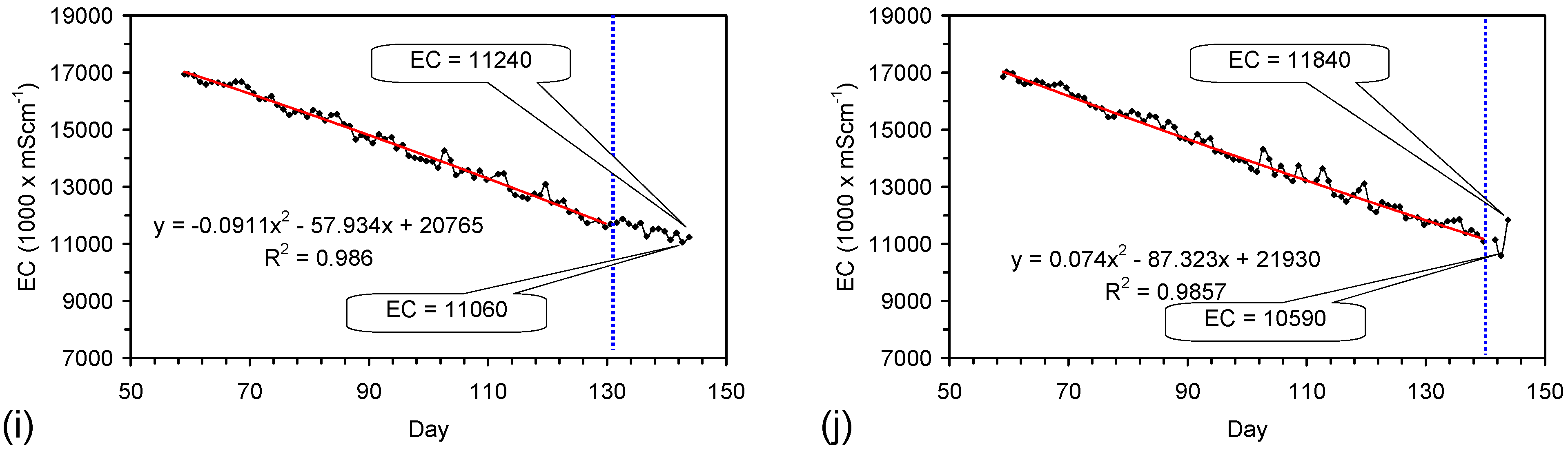
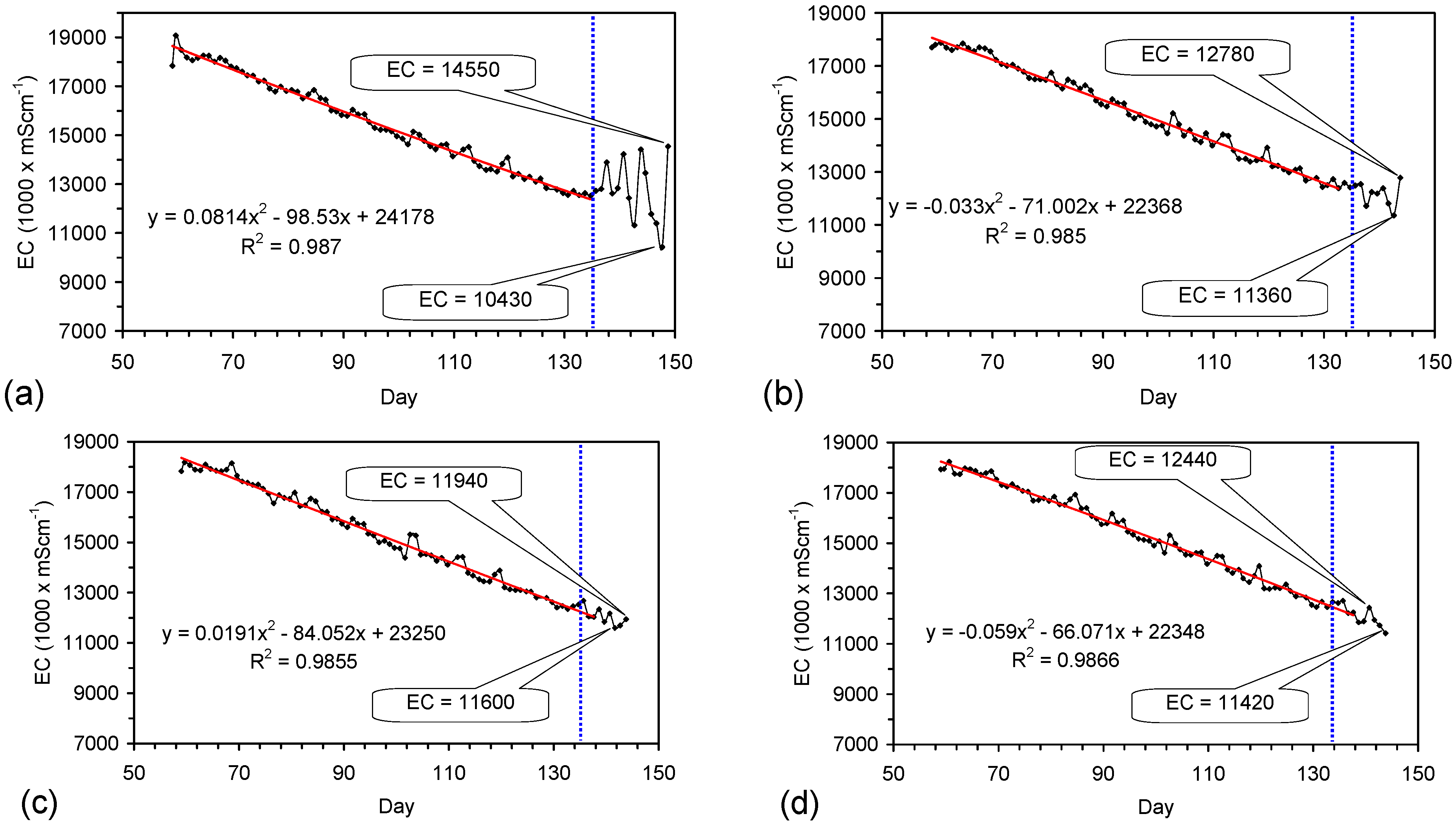
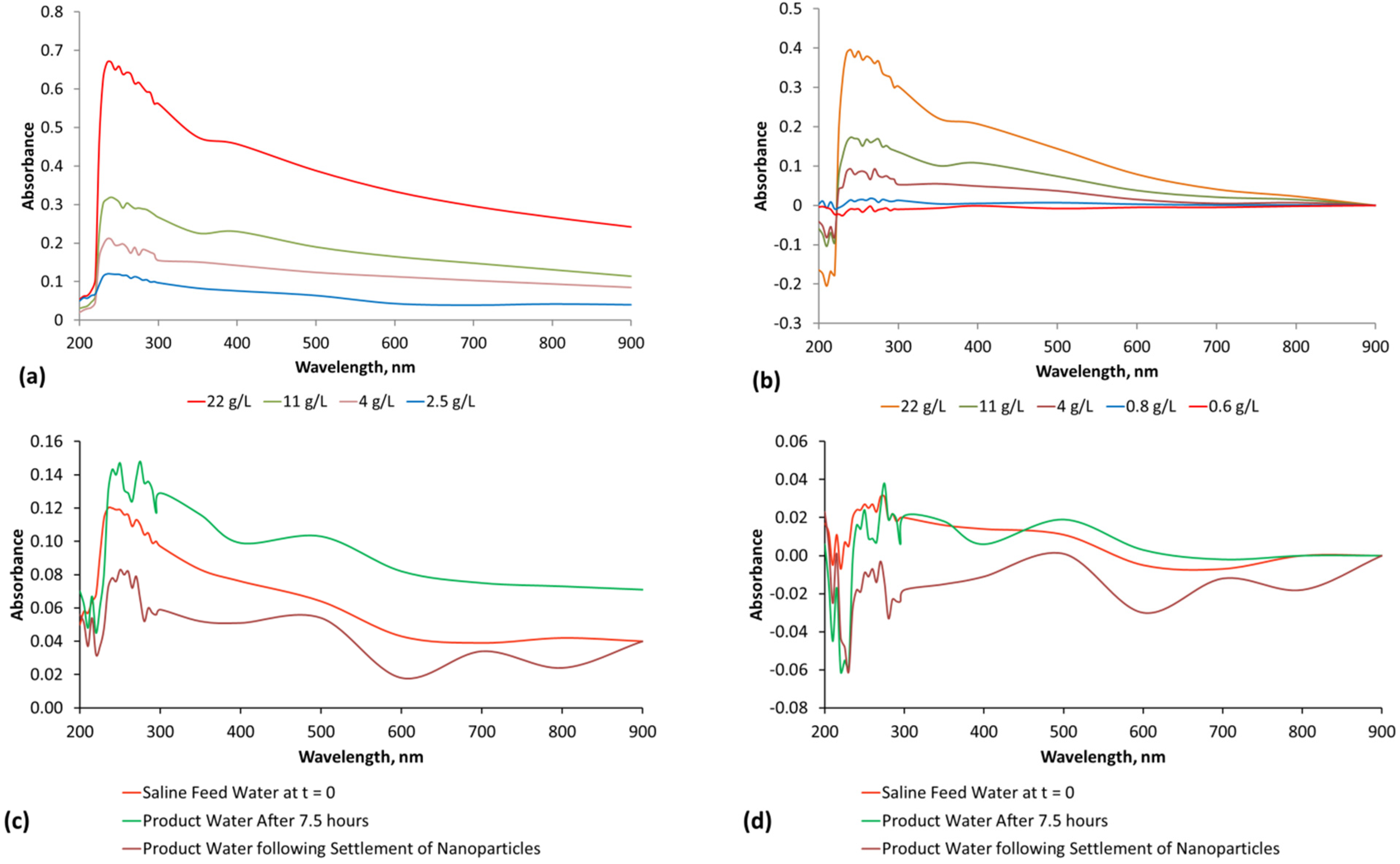
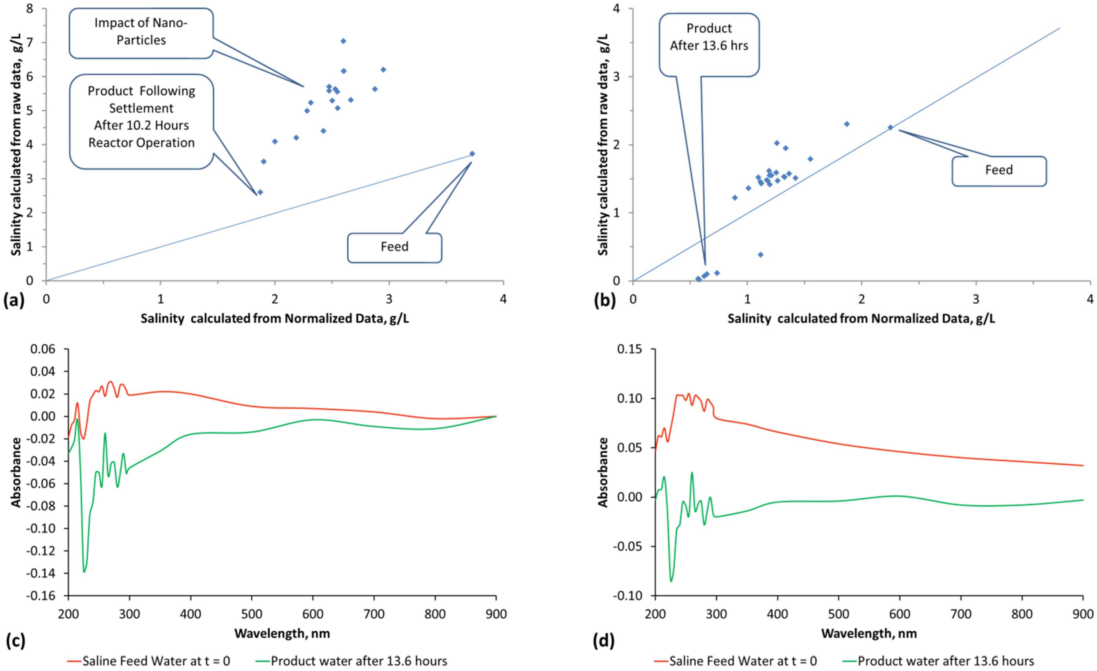
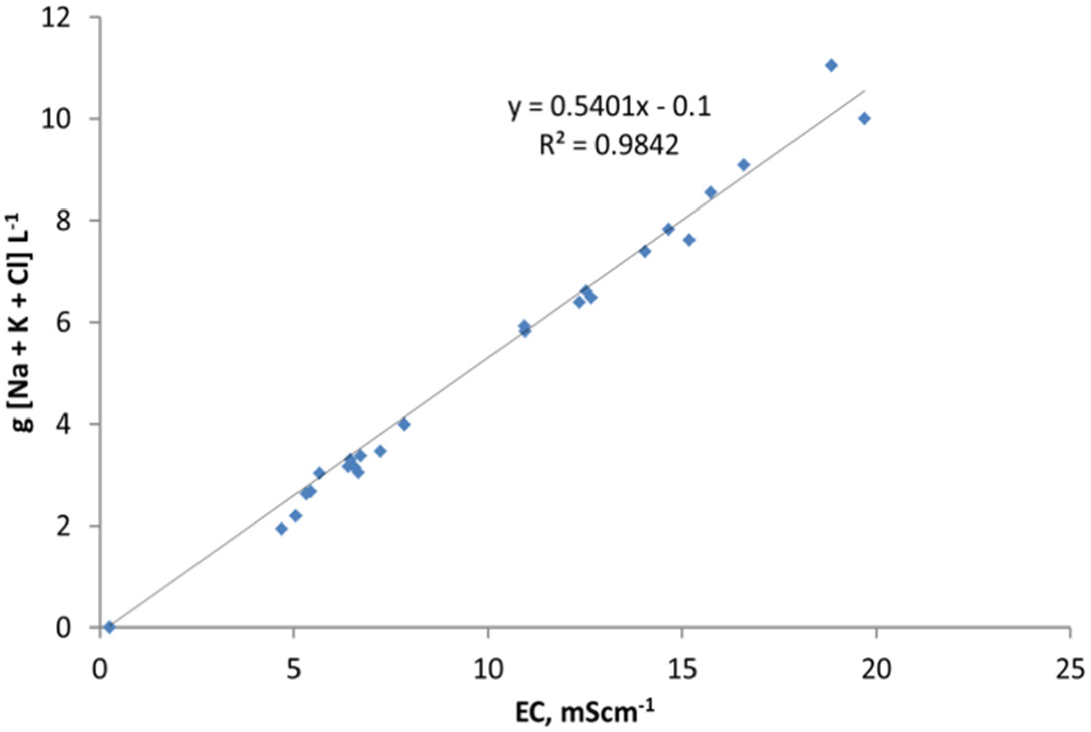
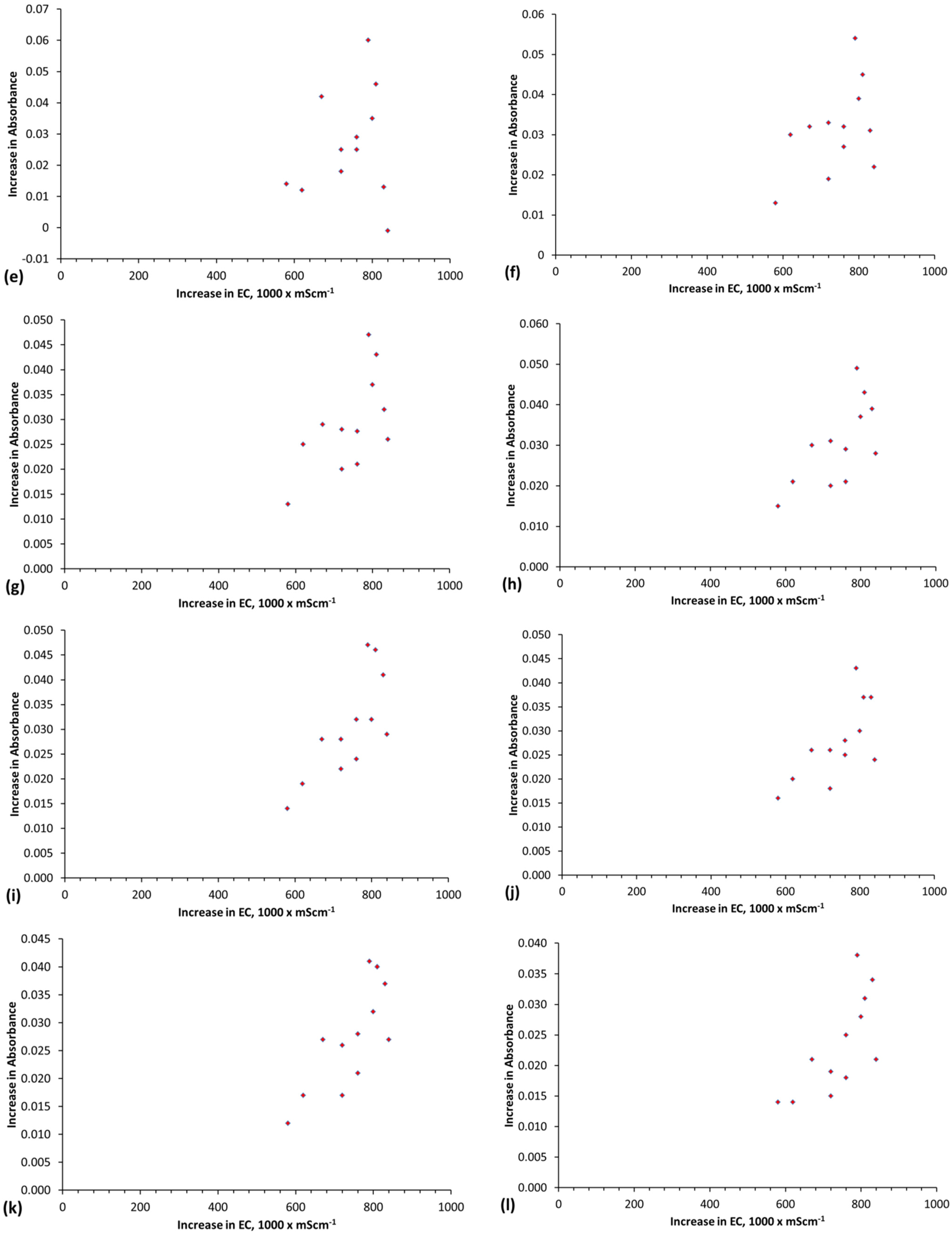
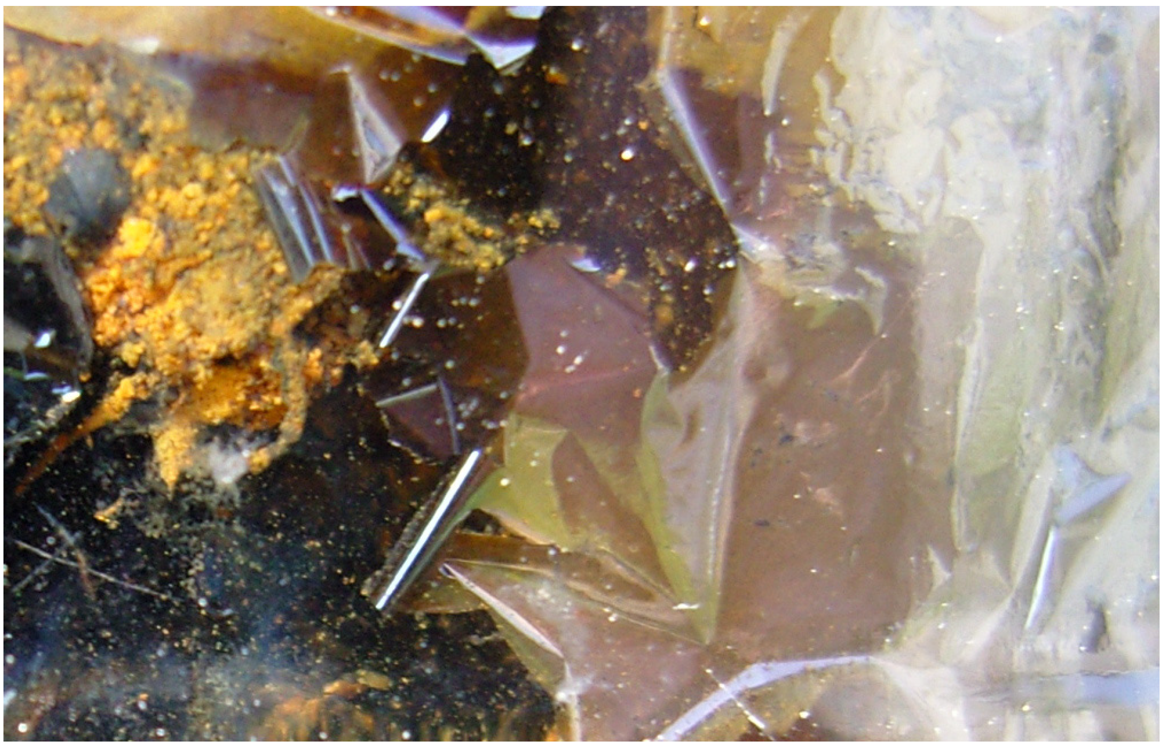
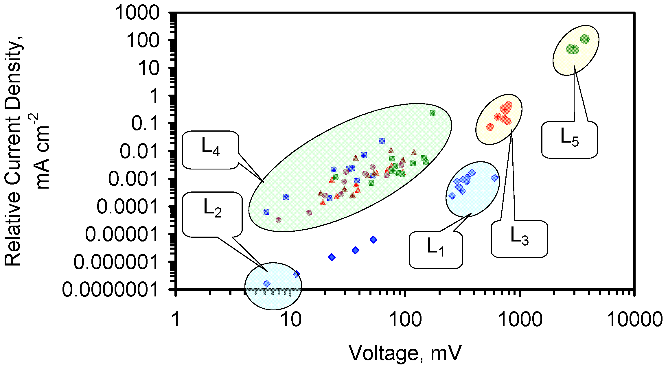
Appendix C. Trial Results
The trial results are placed in Table C1, Table C2, Table C3, Table C4, Table C5, Table C6, Table C7, Table C8, Table C9, Table C10, Table C11, Table C12, Table C13 and Figure C1, Figure C2, Figure C3, Figure C4, Figure C5, Figure C6, Figure C7, Figure C8, Figure C9, Figure C10, Figure C11, Figure C12, Figure C13, Figure C14, Figure C15, Figure C16, Figure C17, Figure C18, Figure C19, Figure C20, Figure C21, Figure C22, Figure C23, Figure C24, Figure C25, Figure C26, Figure C27, Figure C28, Figure C29, Figure C30, Figure C31, Figure C32, Figure C33, Figure C34, Figure C35, Figure C36, Figure C37.
| Water | Cl | N(NO3) | S(SO4) | P(PO4) | F | N(NO2) | Product Water (% Feed Water) | |||
|---|---|---|---|---|---|---|---|---|---|---|
| mg/L | mg/L | mg/L | mg/L | mg/L | mg/L | |||||
| Fresh Spring Water | ||||||||||
| Base Water | 11.67 | 11.28 | 4.16 | <0.10 | 0.024 | 0.04 | - | |||
| PS4 | ||||||||||
| Feed Water | 6004.17 | 11.28 | 4.16 | <0.10 | 0.024 | 0.04 | - | |||
| Product Water | 1434.2 | 0.12 | 3.12 | <0.10 | 0.03 | 2.48 | 55.00% | |||
| PS5 | ||||||||||
| Feed Water | 4568.84 | 11.28 | 4.16 | <0.10 | 0.024 | 0.04 | - | |||
| Product Water | 1613.63 | 0.73 | 2.32 | <0.10 | <0.020 | 3.17 | 55.00% | |||
| PS11 | ||||||||||
| Feed Water | 2464.2 | 1.38 | 1.7 | 0.229 | <0.020 | 2.49 | - | |||
| Product Water | 1554.33 | 1.53 | 2.78 | <0.10 | 0.046 | 2.7 | 92.80% | |||
| PS14 | ||||||||||
| Feed Water | 1914.05 | 10.81 | 4.46 | <0.10 | 0.024 | 3 | - | |||
| Product Water | 1822.42 | 0.13 | 4.84 | <0.10 | 0.024 | 3.22 | 78.30% | |||
| ST3b | ||||||||||
| Feed Water | 6519 | 8.41 | 4.5 | <0.010 | 0.023 | 2.2 | - | |||
| Product Water | 2060 | 0.16 | 1.32 | <0.010 | 0.017 | 1.31 | 75.00% | |||
| ST3f | ||||||||||
| Feed Water | 6519 | 8.41 | 4.5 | <0.010 | 0.023 | 2.2 | - | |||
| Product Water | 2066 | 3.69 | 2.48 | <0.010 | 0.025 | 2.08 | 75.00% | |||
| ST6d | ||||||||||
| Feed Water | 5457.6 | 11.28 | 4.16 | <0.10 | 0.024 | 0.04 | - | |||
| Product Water | 5269.3 | 3.33 | 4.27 | <0.10 | <0.020 | 2.34 | 82.60% | |||
| ST8e | ||||||||||
| Feed Water | 3983.85 | 10.04 | 4.72 | <0.10 | <0.020 | 0.29 | - | |||
| Product Water | 3631.88 | 0.09 | 4.74 | <0.10 | 0.034 | 0.02 | 94.20% | |||
| MT1b | ||||||||||
| Feed Water | 4769 | 11.03 | 4.86 | <0.010 | 0.015 | 1.06 | - | |||
| Product Water | 3937 | 4.61 | 4.58 | <0.010 | 0.067 | 2.21 | 82.60% | |||
| MT2b | ||||||||||
| Feed Water | 4037.39 | 10.5 | 4.51 | <0.10 | <0.020 | <0.020 | - | |||
| Product Water | 3700.83 | 0.53 | 4.49 | <0.10 | <0.020 | 0.08 | 79.20% | |||
| MT3d | ||||||||||
| Feed Water | 2092.1 | 10.81 | 4.55 | 0.436 | <0.020 | 2.4 | - | |||
| Product Water | 1982.02 | 9.77 | 7.35 | <0.10 | 0.079 | 2.43 | 82.60% | |||
| MT4d | ||||||||||
| Feed Water | 2464.2 | 1.38 | 1.7 | 0.229 | <0.020 | 2.49 | - | |||
| Product Water | 1873.3 | 1.39 | 5.5 | <0.10 | 0.041 | 2.42 | 91.30% | |||
| PS15 | ||||||||||
| Feed Water | 16,243.98 | 27.55 | 10.15 | <0.10 | 0.06 | 0.09 | - | |||
| Product Water | 10,076.22 | 3.94 | 6.04 | <0.10 | 0.13 | 2.47 | 66.80% | |||
| PS16 | ||||||||||
| Feed Water | 23,162.04 | 26.03 | 9.59 | <0.10 | 0.06 | 0.09 | - | |||
| Product Water | 348.03 | 0.64 | 1.52 | 0.15 | 0.03 | 0.20 | 26.50% | |||
| Water | K | Ca | Mg | Na | Al | Fe | Mn | |||
|---|---|---|---|---|---|---|---|---|---|---|
| mg/L | mg/L | mg/L | mg/L | µg/L | µg/L | µg/L | ||||
| Fresh Spring Water | ||||||||||
| Base Water | 1.69 | 32.91 | 10.54 | 6.32 | <150.0 | <30.0 | 1.70 | |||
| PS4 | ||||||||||
| Feed Water | 1.69 | 32.91 | 10.54 | 3995.83 | <150.0 | <30.0 | 1.70 | |||
| Product Water | 15.71 | 10.79 | 16.45 | 899.63 | <150.0 | 47.6 | 2.10 | |||
| PS5 | ||||||||||
| Feed Water | 1.69 | 32.91 | 10.54 | 3039.15 | <150.0 | <30.0 | 1.70 | |||
| Product Water | 10.11 | 20.52 | 7.58 | 1009.59 | 173.4 | <30.0 | 5.50 | |||
| PS11 | ||||||||||
| Feed Water | 1.80 | 9.27 | 2.13 | 1522.07 | <150.0 | <30.0 | 2.80 | |||
| Product Water | 2.37 | 3.64 | 44.29 | 1107.61 | <150.0 | <30.0 | 2.10 | |||
| PS14 | ||||||||||
| Feed Water | 2.67 | 31.13 | 9.6 | 1245.32 | <150.0 | <30.0 | 2.80 | |||
| Product Water | 4.92 | 6.94 | 3.58 | 1197.14 | <150.0 | <30.0 | 1.80 | |||
| ST3b | ||||||||||
| Feed Water | 3.49 | 26.65 | 7.65 | 4527 | <150.0 | <30.0 | 8.00 | |||
| Product Water | 5.48 | 3.26 | 2.49 | 1309 | <150.0 | <30.0 | 13.00 | |||
| ST3f | ||||||||||
| Feed Water | 3.49 | 26.65 | 7.65 | 4527 | <150.0 | <30.0 | 8.00 | |||
| Product Water | 7.76 | 17.63 | 7.38 | 1293 | <150.0 | <30.0 | 5.90 | |||
| ST6d | ||||||||||
| Feed Water | 1.69 | 32.91 | 10.54 | 3630.53 | <150.0 | <30.0 | 32.90 | |||
| Product Water | 5.53 | 32.48 | 9.58 | 3275.18 | <150.0 | <30.0 | 69.90 | |||
| ST8e | ||||||||||
| Feed Water | 5.89 | 31.26 | 9.5 | 2390.85 | <150.0 | 34.7 | 14.20 | |||
| Product Water | 6.97 | 14.36 | 4.5 | 2175.29 | <150.0 | <30.0 | 3.30 | |||
| MT1b | ||||||||||
| Feed Water | 2.30 | 31.16 | 9.54 | 3052 | <150.0 | 42.1 | 2.90 | |||
| Product Water | 156.80 | 6.08 | 49.23 | 2521 | 377 | <30.0 | 2.40 | |||
| MT2b | ||||||||||
| Feed Water | 4.18 | 30.17 | 9.09 | 2434.31 | <150.0 | <30.0 | 4.30 | |||
| Product Water | 23.05 | 12.27 | 3.85 | 2198.69 | 2085.2 | <30.0 | 2.90 | |||
| MT3d | ||||||||||
| Feed Water | 2.80 | 30.55 | 9.42 | 1370.7 | <150.0 | <30.0 | 5.10 | |||
| Product Water | 7.04 | 33.65 | 0.41 | 1319.14 | 10,720 | <30.0 | 1.40 | |||
| MT4d | ||||||||||
| Feed Water | 1.80 | 9.27 | 2.13 | 1522.07 | <150.0 | <30.0 | 2.80 | |||
| Product Water | 3.24 | 2.84 | 35.75 | 1273.08 | <150.0 | <30.0 | 2.00 | |||
| PS15 | ||||||||||
| Feed Water | 4087.42 | 80.39 | 25.75 | 8406.66 | <150.0 | <30.0 | 4.15 | |||
| Product Water | 3266.23 | 25.51 | 6.23 | 4197.07 | <150.0 | <30.0 | 23.90 | |||
| PS16 | ||||||||||
| Feed Water | 3.89 | 75.94 | 24.33 | 15,411.17 | <150.0 | <30.0 | 3.92 | |||
| Product Water | 5.24 | 7.46 | 1.82 | 223.21 | 288.8 | <30.0 | 4.00 | |||
| Water | P | S | B | Ba | Cd | Co | Cr |
|---|---|---|---|---|---|---|---|
| mg/L | mg/L | µg/L | µg/L | µg/L | µg/L | µg/L | |
| Fresh Spring Water | |||||||
| Base Water | <0.005 | 4.31 | 29.40 | 135.60 | <0.2 | <0.2 | <2.0 |
| PS4 | |||||||
| Feed Water | <0.005 | 4.31 | 29.40 | 135.60 | <0.2 | <0.2 | <2.0 |
| Product Water | 0.01 | 3.3 | 12.00 | 15.10 | <0.2 | 1.30 | <2.0 |
| PS5 | |||||||
| Feed Water | <0.005 | 4.31 | 29.40 | 135.60 | <0.2 | <0.2 | <2.0 |
| Product Water | 0.01 | 2.55 | <10 | <15 | <0.2 | 1.50 | <2.0 |
| PS11 | |||||||
| Feed Water | 0.25 | 1.89 | <10 | 16.40 | <0.2 | 1.80 | <2.0 |
| Product Water | 0.04 | 3.15 | 25.80 | <15 | <0.2 | 1.40 | <2.0 |
| PS14 | |||||||
| Feed Water | 0.03 | 4.51 | 22.20 | 117.10 | <0.2 | 1.50 | <2.0 |
| Product Water | 0.01 | 4.8 | <10 | <15 | <0.2 | 1.50 | <2.0 |
| ST3b | |||||||
| Feed Water | 0.07 | 4.59 | 14.90 | 103.10 | 0.9 | 3.30 | <2.0 |
| Product Water | 0.01 | 1.56 | 59.40 | <15.0 | 1.2 | 1.20 | <2.0 |
| ST3f | |||||||
| Feed Water | 0.07 | 4.59 | 14.90 | 103.10 | 0.9 | 3.30 | <2.0 |
| Product Water | 0.02 | 2.63 | 17.50 | <15.0 | 1.0 | 1.60 | <2.0 |
| ST6d | |||||||
| Feed Water | <0.005 | 4.31 | 29.40 | 135.60 | <0.2 | <0.2 | <2.0 |
| Product Water | 0.01 | 4.31 | <10 | 68.50 | <0.2 | 3.90 | <2.0 |
| ST8e | |||||||
| Feed Water | 0.01 | 4.8 | 28.90 | 118.70 | <0.2 | 2.20 | <2.0 |
| Product Water | 0.01 | 4.9 | 34.60 | <15 | <0.2 | 1.10 | <2.0 |
| MT1b | |||||||
| Feed Water | 0.04 | 4.79 | 20.80 | 102.80 | 0.4 | 1.30 | <2.0 |
| Product Water | 0.01 | 4.79 | 70.40 | <15.0 | 0.4 | 1.60 | <2.0 |
| MT2b | |||||||
| Feed Water | 0.02 | 4.66 | 15.80 | 115.40 | <0.2 | 2.40 | <2.0 |
| Product Water | 0.01 | 4.68 | 11.30 | <15 | <0.2 | 2.20 | <2.0 |
| MT3d | |||||||
| Feed Water | 0.47 | 4.66 | 36.00 | 118.90 | 0.3 | 0.80 | <2.0 |
| Product Water | 0.03 | 7.55 | 22.30 | <15 | <0.2 | 1.80 | <2.0 |
| MT4d | |||||||
| Feed Water | 0.25 | 1.89 | <10 | 16.40 | <0.2 | 1.80 | <2.0 |
| Product Water | 0.02 | 6.02 | 97.30 | <15 | <0.2 | 2.40 | <2.0 |
| PS15 | |||||||
| Feed Water | <0.005 | 10.52 | 71.82 | 331.20 | <0.2 | <0.2 | <2.0 |
| Product Water | 0.01 | 6.12 | 38.10 | 55.20 | 10.2 | 3.60 | <2.0 |
| PS16 | |||||||
| Feed Water | <0.005 | 9.94 | 67.80 | 312.90 | <0.2 | <0.2 | <2.0 |
| Product Water | <0.005 | 3.74 | 109.60 | <15 | <0.2 | 0.20 | <2.0 |
| Water | Cu | Ni | Pb | Si | Sr | Zn | As |
|---|---|---|---|---|---|---|---|
| µg/L | µg/L | µg/L | mg/L | µg/L | µg/L | µg/L | |
| Fresh Spring Water | |||||||
| Base Water | 77.7 | <3 | <10 | 5.21 | 144.9 | 37.4 | |
| PS4 | |||||||
| Feed Water | 77.7 | <3 | <10 | 5.21 | 144.9 | 37.4 | |
| Product Water | <20 | <3 | <10 | 0.05 | 76 | <4 | |
| PS5 | |||||||
| Feed Water | 77.7 | <3 | <10 | 5.21 | 144.9 | 37.4 | |
| Product Water | 54.3 | <3 | <10 | 0.09 | 54.2 | 33.8 | |
| PS11 | |||||||
| Feed Water | <20 | <3 | <10 | 1.43 | 28.5 | 137.5 | |
| Product Water | <20 | <3 | <10 | 0.9 | 4.3 | 14.1 | |
| PS14 | |||||||
| Feed Water | 122.1 | <3 | <10 | 4.77 | 136.1 | 125.6 | |
| Product Water | <20 | <3 | <10 | 0.04 | 54 | <4 | |
| ST3b | |||||||
| Feed Water | 45.1 | 3.7 | <10 | 3.99 | 112.4 | 337.6 | 2.3 |
| Product Water | <20.0 | <3.0 | <10 | 0.29 | 15.6 | <4.00 | 5.4 |
| ST3f | |||||||
| Feed Water | 45.1 | 3.7 | <10 | 3.99 | 112.4 | 337.6 | 2.3 |
| Product Water | <20.0 | <3.0 | <10 | 0.62 | 103.4 | <4.00 | 5.3 |
| ST6d | |||||||
| Feed Water | 77.7 | <3 | <10 | 5.21 | 144.9 | 37.4 | - |
| Product Water | 736.5 | <3 | <10 | 0.41 | 134.6 | 68.2 | - |
| ST8e | |||||||
| Feed Water | 41 | <3 | <10 | 4.89 | 138 | 286.9 | - |
| Product Water | <20 | <3 | <10 | 0.28 | 32.5 | 29 | - |
| MT1b | |||||||
| Feed Water | 52.9 | <3.0 | <10 | 4.92 | 139.9 | 170 | 4.8 |
| Product Water | <20.0 | <3.0 | <10 | 0.37 | 6.7 | 17.6 | 2.5 |
| MT2b | |||||||
| Feed Water | 93.1 | <3 | <10 | 4.67 | 133.3 | 101.1 | - |
| Product Water | <20 | <3 | <10 | 0.06 | 10.2 | 5.1 | - |
| MT3d | |||||||
| Feed Water | 74.9 | <3 | <10 | 4.83 | 134.3 | 342 | - |
| Product Water | <20 | <3 | <10 | 0.12 | 209.1 | <4 | - |
| MT4d | |||||||
| Feed Water | <20 | <3 | <10 | 1.43 | 28.5 | 137.5 | - |
| Product Water | <20 | <3 | <10 | 0.44 | 0.8 | 7.7 | - |
| PS15 | |||||||
| Feed Water | 189.80 | <3 | <10 | 12.73 | 353.9 | 91.36 | - |
| Product Water | 31.80 | <3 | <10 | 0.22 | 86.1 | 205.10 | - |
| PS16 | |||||||
| Feed Water | 179.30 | <3 | <10 | 12.03 | 334.4 | 86.30 | - |
| Product Water | 29.00 | <3 | <10 | 0.35 | 30.6 | 828.50 | - |
| Trial | Water Charge | Feed Water | Eh, mV | pH | EC, mS·cm−1 |
|---|---|---|---|---|---|
| L | NaCl, g·L−1 | ||||
| E143a | 5.4 | 5.74 | 0.2 | 5.66 | 11.15 |
| E143b | 5.4 | 4.44 | 0.193 | 6.61 | 8.63 |
| E143c | 5.4 | 4.81 | 0.199 | 6.11 | 9.35 |
| E143d | 5.4 | 5.37 | 0.214 | 5.59 | 10.43 |
| E143e | 5.4 | 6.48 | 0.22 | 5.78 | 12.59 |
| E143f | 5.4 | 1.85 | 0.166 | 5.65 | 3.59 |
| E143g | 5.4 | 2.59 | 0.188 | 6.46 | 5.04 |
| E143h | 5.4 | 2.63 | 0.176 | 6.46 | 5.04 |
| E143i | 5.4 | 2.96 | 0.185 | 6.18 | 5.75 |
| E143j | 5.4 | 3.33 | 0.17 | 5.18 | 6.63 |
| E143k | 5.4 | 3.35 | 0.219 | 6.19 | 6.63 |
| Trial | Eh, mV | pH | EC, mS·cm−1 | Storage | Stored Water Analysis | pH | EC, mS·cm−1 |
|---|---|---|---|---|---|---|---|
| Weeks | Eh, mV | ||||||
| E143a | 0.214 | 6.80 | 0.725 | 6 | 0.232 | 6.82 | 0.814 |
| E143b | 0.226 | 6.19 | 3.29 | 4 | 0.214 | 7.00 | 3.62 |
| E143c | 0.248 | 5.22 | 4.10 | 4 | 0.227 | 6.86 | 4.25 |
| E143d | 0.258 | 5.31 | 5.73 | 4 | 0.243 | 6.51 | 5.80 |
| E143e | 0.224 | 5.54 | 9.35 | 4 | 0.238 | 6.58 | 9.57 |
| E143f | 0.185 | 6.68 | 6.71 | 4 | 0.220 | 6.96 | 7.01 |
| E143g | 0.197 | 6.76 | 4.70 | 4 | 0.215 | 7.13 | 4.75 |
| E143h | 0.201 | 6.90 | 6.27 | 4 | 0.219 | 7.05 | 6.28 |
| E143i | 0.165 | 5.12 | 9.51 | 4 | 0.261 | 6.13 | 9.52 |
| E143j | 0.212 | 5.31 | 6.15 | 4 | 0.271 | 6.17 | 6.19 |
| E143k | 0.207 | 6.04 | 6.56 | 4 | 0.261 | 6.34 | 6.47 |
Table C7.
ZVM TPA Example (Trial E143): Product Water Volume Recovered, Trial Duration, Temperature, Gas Flows.
| Trial | Water Recovered | Water Consumed | Duration | Air Flow | CO2 Flow | Air Flow Rate | CO2 Flow Rate | Temperature |
|---|---|---|---|---|---|---|---|---|
| L | L | h | h | h | L·h−1 | L·h−1 | ||
| E143a | 4.60 | 0.80 | 9.00 | 9.00 | 0.00 | 13.2 | 3.3 | 5–12 °C |
| E143b | 4.60 | 0.80 | 8.33 | 5.05 | 3.28 | 13.2 | 3.3 | 5–10 °C |
| E143c | 4.70 | 0.70 | 4.37 | 2.56 | 1.81 | 13.2 | 3.3 | 5–10 °C |
| E143d | 4.80 | 0.60 | 4.02 | 1.76 | 2.26 | 13.2 | 3.3 | 5–10 °C |
| E143e | 4.70 | 0.70 | 3.87 | 1.71 | 2.16 | 13.2 | 3.3 | 5–10 °C |
| E143f | 4.65 | 0.75 | 2.70 | 2.70 | 0.00 | 13.2 | 3.3 | 5–10 °C |
| E143g | 4.50 | 0.90 | 3.08 | 3.08 | 0.00 | 13.2 | 3.3 | 5–10 °C |
| E143h | 3.90 | 1.50 | 14.30 | 14.30 | 0.00 | 13.2 | 3.3 | 5–10 °C |
| E143i | 4.00 | 1.40 | 8.90 | 4.50 | 4.40 | 13.2 | 3.3 | 5–10 °C |
| E143j | 3.90 | 1.50 | 7.50 | 2.20 | 5.30 | 13.2 | 3.3 | 5–10 °C |
| E143k | 3.90 | 1.50 | 3.58 | 2.58 | 1.00 | 13.2 | 3.3 | 5–10 °C |
Table C8.
ZVM TPA Example (Trial E143): Salinity Changes calculated from changes in EC and changes in water volume.
| Trial | Product Water | Apparent NaCl Removed | Actual NaCl Removed | Cumulative NaCl Removed | Cumulative Water Processed | Cumulative |
|---|---|---|---|---|---|---|
| g·L−1 | g·L−1 | g·L−1 | g·L−1 | L | NaCl in Feed g·L−1 | |
| E143a | 0.064 | 5.68 | 5.686 | 5.69 | 5.4 | 5.74 |
| E143b | 1.514 | 2.93 | 3.154 | 8.84 | 10.8 | 10.19 |
| E143c | 1.933 | 2.88 | 3.132 | 11.97 | 16.2 | 15.00 |
| E143d | 2.786 | 2.58 | 2.894 | 14.87 | 21.6 | 20.37 |
| E143e | 4.686 | 1.80 | 2.403 | 17.27 | 27.0 | 26.85 |
| E143f | 3.491 | −1.64 | −1.154 | 16.12 | 32.4 | 28.70 |
| E143g | 2.363 | 0.23 | 0.623 | 16.74 | 37.8 | 31.30 |
| E143h | 3.248 | −0.62 | 0.284 | 17.02 | 43.2 | 33.93 |
| E143i | 4.948 | −1.98 | −0.702 | 16.32 | 48.6 | 36.89 |
| E143j | 3.028 | 0.31 | 1.146 | 17.47 | 54.0 | 40.22 |
| E143k | 3.268 | 0.08 | 0.992 | 18.46 | 59.4 | 43.57 |
| Trial | Water Charge, L | Feed Water | Eh, mV | pH | EC, mS·cm−1 |
|---|---|---|---|---|---|
| NaCl, g·L−1 | |||||
| E144a | 5.4 | 4.07 | 0.203 | 6.50 | 7.91 |
| E144b | 5.4 | 4.07 | 0.192 | 6.35 | 7.94 |
| E144c | 5.4 | 1.00 | 0.181 | 6.31 | 2.16 |
| E144d | 5.4 | 1.10 | 0.191 | 6.16 | 2.34 |
| E144e | 5.4 | 2.05 | 0.218 | 6.37 | 4.04 |
| E144f | 5.4 | 5.83 | 0.192 | 6.34 | 11.25 |
| Trial | Eh, mV | pH | EC, mS·cm−1 | Storage Weeks | Stored Water Analysis | pH | EC, mS·cm−1 |
|---|---|---|---|---|---|---|---|
| Eh, mV | |||||||
| E144a | 0.199 | 5.64 | 7.03 | 3 | 0.282 | 6.51 | 5.8 |
| E144b | 0.222 | 6.64 | 7.32 | 3 | 0.282 | 6.57 | 6.6 |
| E144c | 0.154 | 5.23 | 3.92 | - | - | - | - |
| E144d | 0.169 | 5.38 | 2.74 | - | - | - | - |
| E144e | 0.153 | 5.30 | 4.08 | - | - | - | - |
| E144f | 0.080 | 5.56 | 8.58 | - | - | - | - |
Table C11.
ZVM TPA Example (Trial E144): Product Water Volume Recovered, Trial Duration, Temperature, Gas Flows.
| Trial | Water Recovered | Water Consumed | Duration | Air Flow | CO2 Flow | Air Flow Rate | CO2 Flow Rate | Temperature |
|---|---|---|---|---|---|---|---|---|
| L | L | h | h | h | L·h−1 | L·h−1 | °C | |
| E144a | 4.00 | 1.40 | 5.1 | 3.8 | 1.3 | 13.2 | 3.3 | 5–12 |
| E144b | 4.00 | 1.40 | 104.3 | 70.5 | 33.8 | 13.2 | 3.3 | 8–15 |
| E144c | 4.50 | 0.90 | 690.0 | 0.0 | 690.0 | 13.2 | 3.3 | 11–15 |
| E144d | 4.15 | 1.25 | 291.0 | 0.0 | 291.0 | 13.2 | 3.3 | 12–16 |
| E144e | 4.00 | 1.40 | 537.0 | 0.0 | 537.0 | 13.2 | 3.3 | 16–19 |
| E144f | 3.50 | 1.90 | 1295.0 | 0.0 | 1295.0 | 13.2 | 3.3 | 13–19 |
Table C12.
ZVM TPA Example (Trial E144): Salinity changes calculated from changes in EC, spectrometry, and changes in water volume.
| Trial | Product Water Salinity Based on EC | Product Water Salinity Based on Spectrometry | Apparent NaCl Removed | Actual NaCl Removed | Cumulative NaCl Removed | Cumulative Water Processed | Cumulative |
|---|---|---|---|---|---|---|---|
| g·L−1 | g·L−1 | g·L−1 | g·L−1 | g·L−1 | NaCl in feed g·L−1 | ||
| E144a | 3.55 | - | 0.52 | 1.44 | 1.44 | 5.4 | 4.07 |
| E144b | 3.69 | - | 0.38 | 1.34 | 2.78 | 10.8 | 8.15 |
| E144c | 1.90 | 0.53 | 0.47 | 0.56 | 3.34 | 16.2 | 9.15 |
| E144d | 1.27 | 1.04 | 0.06 | 0.30 | 3.64 | 21.6 | 10.25 |
| E144e | 2.03 | 1.30 | 0.75 | 1.09 | 4.73 | 27.0 | 12.30 |
| E144f | 4.35 | 2.77 | 3.06 | 4.04 | 8.77 | 32.4 | 18.13 |
Table C13.
ZVM TPA Example (Trial E146): Feed Water and Product Water Composition. The NaCl in the feed water is dissolved halite (Cheshire). The product water contains a settled layer of precipitant including clays and Fe hydroxides/peroxides derived from the halite. The apparent increase in salinity in Trial E146l is due to the rate of nano-particle formation exceeding the rate of desalination.
| Trial | Water Charge, L | Feed Water | Eh, mV | pH | EC, mS·cm−1 | Product Water | pH | EC, mS·cm−1 | NaCl, g·L−1 | Desalination | |
|---|---|---|---|---|---|---|---|---|---|---|---|
| NaCl, g·L−1 | Eh, mV | NaCl, g·L−1 | |||||||||
| E146a | 240 | 1.38 | 0.188 | 6.83 | 2.88 | 0.152 | 8.01 | 4.24 | 1.04 | 0.34 | |
| E146b | 240 | 2.73 | 0.164 | 6.67 | 5.4 | 0.151 | 8.31 | 5.35 | 2.09 | 0.64 | |
| E146c | 240 | 3.76 | 0.202 | 6.92 | 7.34 | 0.172 | 8.29 | 10.16 | 0.64 | 3.12 | |
| E146d | 240 | 6.27 | 0.156 | 6.99 | 12.2 | 0.178 | 8.27 | 18.19 | 4.68 | 1.59 | |
| E146e | 240 | 2.92 | 0.196 | 6.96 | 5.76 | 0.156 | 8.10 | 6.51 | 1.96 | 0.96 | |
| E146f | 240 | 2.24 | 0.162 | 6.90 | 4.47 | 0.142 | 8.19 | 5.29 | 1.39 | 0.85 | |
| E146g | 240 | 2.45 | 0.164 | 6.89 | 4.94 | 0.145 | 8.15 | 5.73 | 0.71 | 1.74 | |
| E146h | 240 | 3.73 | 0.164 | 6.97 | 7.39 | 0.157 | 8.37 | 8.62 | 1.87 | 1.86 | |
| E146i | 240 | 2.25 | 0.164 | 7.08 | 4.56 | 0.134 | 8.57 | 4.84 | 0.62 | 1.63 | |
| E146j | 240 | 2.75 | 0.176 | 6.19 | 5.48 | 0.155 | 7.57 | 5.57 | 1.85 | 0.90 | |
| E146k | 240 | 2.07 | 0.176 | 6.34 | 4.25 | 0.174 | 7.50 | 4.59 | 0.69 | 1.38 | |
| E146l | 240 | 1.39 | 0.181 | 6.24 | 2.9 | 0.173 | 7.65 | 3.69 | 2.73 | −1.34 | |
| E146m | 240 | 2.17 | 0.181 | 6.33 | 4.38 | 0.174 | 7.50 | 4.59 | 0.61 | 1.56 | |
| E146n | 240 | 1.00 | 0.181 | 6.31 | 2.26 | 0.117 | 6.86 | 2.86 | 0.5 | 0.50 | |
| E146o | 240 | 1.10 | 0.191 | 6.16 | 2.34 | 0.134 | 7.10 | 3.14 | 0.76 | 0.34 | |
| E146p | 240 | 2.05 | 0.218 | 6.37 | 4.04 | 0.129 | 7.05 | 4.77 | 1.65 | 0.40 | |
| E146q | 240 | 5.83 | 0.192 | 6.35 | 11.25 | 0.099 | 7.40 | 12.27 | 2.15 | 3.68 | |
Figure C1.
(a) EC vs. day; (b) Eh vs. day; (c) pH vs. day; (d) pH vs. Eh. ZVM TP = particulate material placed in water at a concentration of PS1 = 30 g·L−1; PS2 = 30 g·L−1; PS3 = 65 g·L−1; PS4 = 55 g·L−1. Reactor Size: 0.3 L; Feed Water volume: 0.2 L.
Figure C1.
(a) EC vs. day; (b) Eh vs. day; (c) pH vs. day; (d) pH vs. Eh. ZVM TP = particulate material placed in water at a concentration of PS1 = 30 g·L−1; PS2 = 30 g·L−1; PS3 = 65 g·L−1; PS4 = 55 g·L−1. Reactor Size: 0.3 L; Feed Water volume: 0.2 L.
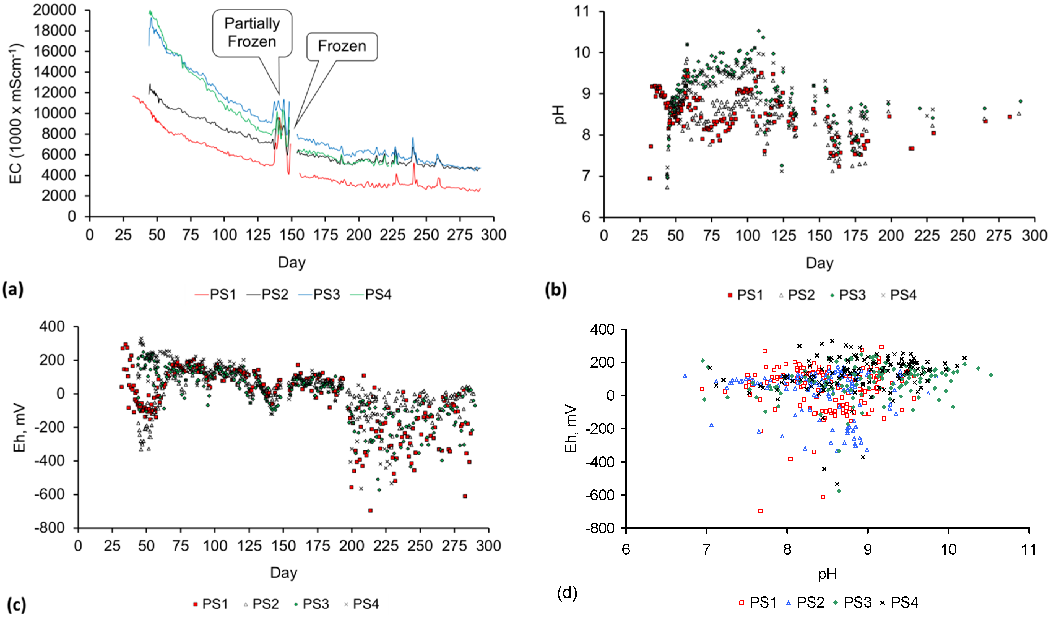
Figure C2.
(a) EC vs. day; (b) Eh vs. day; (c) pH vs. day; (d) pH vs. Eh; ZVM TP = particulate material placed in water at a concentration of PS5 = 30 g·L−1; PS8 = 30 g·L−1; PS9 = 60 g·L−1; Reactor Size: 0.3 L; Feed Water volume: 0.2 L.
Figure C2.
(a) EC vs. day; (b) Eh vs. day; (c) pH vs. day; (d) pH vs. Eh; ZVM TP = particulate material placed in water at a concentration of PS5 = 30 g·L−1; PS8 = 30 g·L−1; PS9 = 60 g·L−1; Reactor Size: 0.3 L; Feed Water volume: 0.2 L.


Figure C3.
(a) EC vs. day; (b) Eh vs. day; (c) pH vs. day; (d) pH vs. Eh. ZVM TP = particulate material placed in water at a concentration of PS11 = 26.5 g·L−1; PS12 = 14.3 g·L−1; PS13 = 5.65 g·L−1; PS14 = 10.2 g·L−1. Reactor Size: 2.3 L; Feed Water volume: 2.3 L.
Figure C3.
(a) EC vs. day; (b) Eh vs. day; (c) pH vs. day; (d) pH vs. Eh. ZVM TP = particulate material placed in water at a concentration of PS11 = 26.5 g·L−1; PS12 = 14.3 g·L−1; PS13 = 5.65 g·L−1; PS14 = 10.2 g·L−1. Reactor Size: 2.3 L; Feed Water volume: 2.3 L.
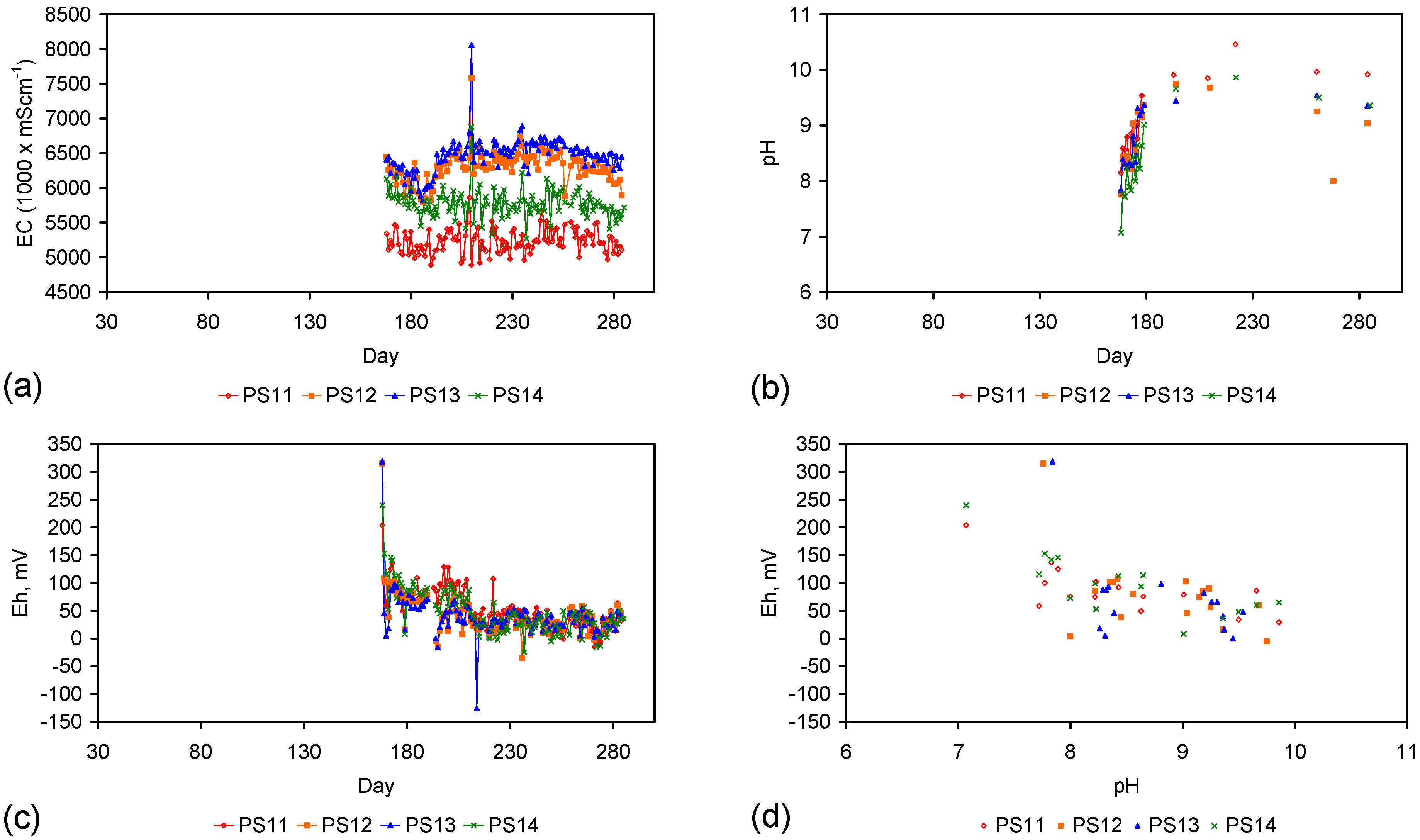
Figure C4.
(a) EC vs. day; (b) Eh vs. day; (c) pH vs. day; (d) pH vs. Eh. AS4 = 42 g·L−1; AS5 = 59 g·L−1; AS6 = 35 g·L−1. Reactor Size: 0.3 L; Feed Water volume: 0.2 L.
Figure C4.
(a) EC vs. day; (b) Eh vs. day; (c) pH vs. day; (d) pH vs. Eh. AS4 = 42 g·L−1; AS5 = 59 g·L−1; AS6 = 35 g·L−1. Reactor Size: 0.3 L; Feed Water volume: 0.2 L.
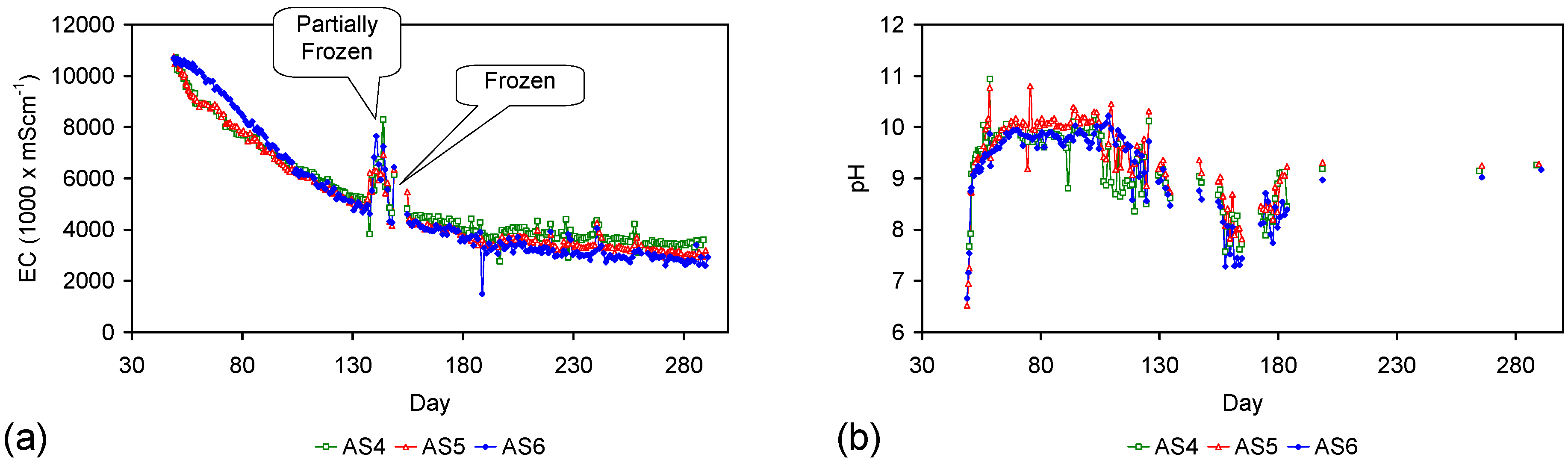

Figure C5.
(a) pH vs. Eh; (b) EC vs. day, ST1a–ST1e; (c) EC vs. day, ST1f–ST1j; (d) pH vs. day, ST1a–ST1e; (e) pH vs. day; ST1f–ST1j; (f) Eh vs. day, ST1a–ST1e; (g) Eh vs. day, ST1f–ST1j. ZVM TP = copper sheathed pellets (15 mm OD) placed in water at a concentration of ST1a = 18.3 g·L−1; ST1b = 23.1 g·L−1; ST1c = 25.3 g·L−1; ST1d = 26.7 g·L−1; ST1e = 21.7 g·L−1; ST1f = 28.3 g·L−1; ST1g = 31.9 g·L−1; ST1h = 30.1 g·L−1; ST1i = 23.3 g·L−1; ST1j = 25.1 g·L−1. Reactor Size: 0.3 L; Feed Water volume: 0.2 L.

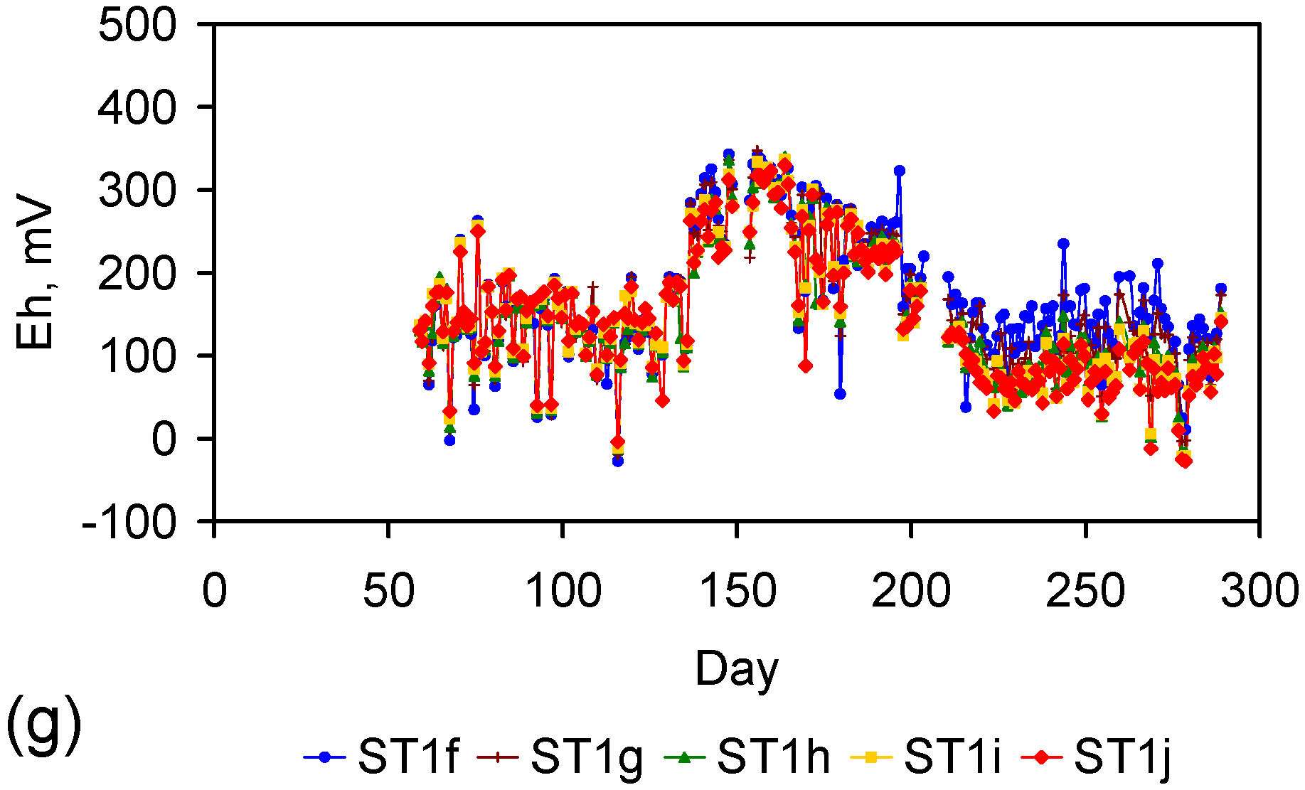
Figure C6.
(a) pH vs. Eh; (b) EC vs. day, ST2a–ST2e; (c) EC vs. day, ST2f–ST2j; (d) pH vs. day, ST2a–ST2e; (e) pH vs. day, ST2f–ST2j; (f) Eh vs. day, ST2a–ST2e; (g) Eh vs. day, ST2f–ST2j. ZVM TP = copper sheathed pellets (15 mm OD) placed in water at a concentration of ST2a = 28.5 g·L−1; ST2b = 30 g·L−1; ST2c = 25 g·L−1; ST2d = 25 g·L−1; ST2e = 33.5 g·L−1; ST2f = 26.5 g·L−1; ST2g = 26.5 g·L−1; ST2h = 23.5 g·L−1; ST2i = 26.5 g·L−1; ST2j = 33.5 g·L−1. Reactor Size: 0.3 L; Feed Water volume: 0.2 L.


Figure C7.
(a) pH vs. Eh; (b) EC vs. day, ST3a–ST3e; (c) EC vs. day, ST3f–ST3j; (d) pH vs. day, ST3a–ST3e; (e) pH vs. day, ST3f–ST3j; (f) Eh vs. day, ST3a–ST3e; (g) Eh vs. day, ST3f–ST3j. ZVM TP = copper sheathed pellets (15 mm OD) placed in water at a concentration of ST3a = 32 g·L−1; ST3b = 25 g·L−1; ST3c = 30 g·L−1; ST3d = 30 g·L−1; ST3e = 26.5 g·L−1; ST3f = 57.5 g·L−1; ST3g = 82.5 g·L−1; ST3h = 65 g·L−1; ST3i = 72 g·L−1; ST3j = 66.5 g·L−1. Reactor Size: 0.3 L; Feed Water volume: 0.2 L.


Figure C8.
(a) pH vs. Eh; (b) EC vs. day, ST4a–ST4e; (c) EC vs. day, ST4f–ST4j; (d) pH vs. day, ST4a–ST4e; (e) pH vs. day, ST4f–ST4j; (f) Eh vs. day, ST4a–ST4e; (g) Eh vs. day, ST4f–ST4j. ZVM TP = copper sheathed pellets (15 mm OD) placed in water at a concentration of ST4a = 50 g·L−1; ST4b = 55.5 g·L−1; ST4c = 50 g·L−1; ST4d = 63.5 g·L−1; ST4e = 87.5 g·L−1; ST4f = 44 g·L−1; ST4g = 49 g·L−1; ST4h = 66.5 g·L−1; ST4i = 36 g·L−1; ST4j = 44.5 g·L−1. Reactor Size: 0.3 L; Feed Water volume: 0.2 L.


Figure C9.
(a) pH vs. Eh; (b) EC vs. day, ST5a–ST5e; (c) EC vs. day, ST5f–ST5j; (d) pH vs. day, ST5a–ST5e; (e) pH vs. day, ST5f–ST5j; (f) Eh vs. day, ST5a–ST5e; (g) Eh vs. day, ST5f–ST5j. ZVM TP = copper sheathed pellets (15 mm OD) placed in water at a concentration of ST5a = 64 g·L−1; ST5b = 47.5 g·L−1; ST5c = 48 g·L−1; ST5d = 62.5 g·L−1; ST5e = 94 g·L−1; ST5f = 47.5 g·L−1; ST5g = 38 g·L−1; ST5h = 46 g·L−1; ST5i = 39.5 g·L−1; ST5j = 72.5 g·L−1. Reactor Size: 0.3 L; Feed Water volume: 0.2 L.

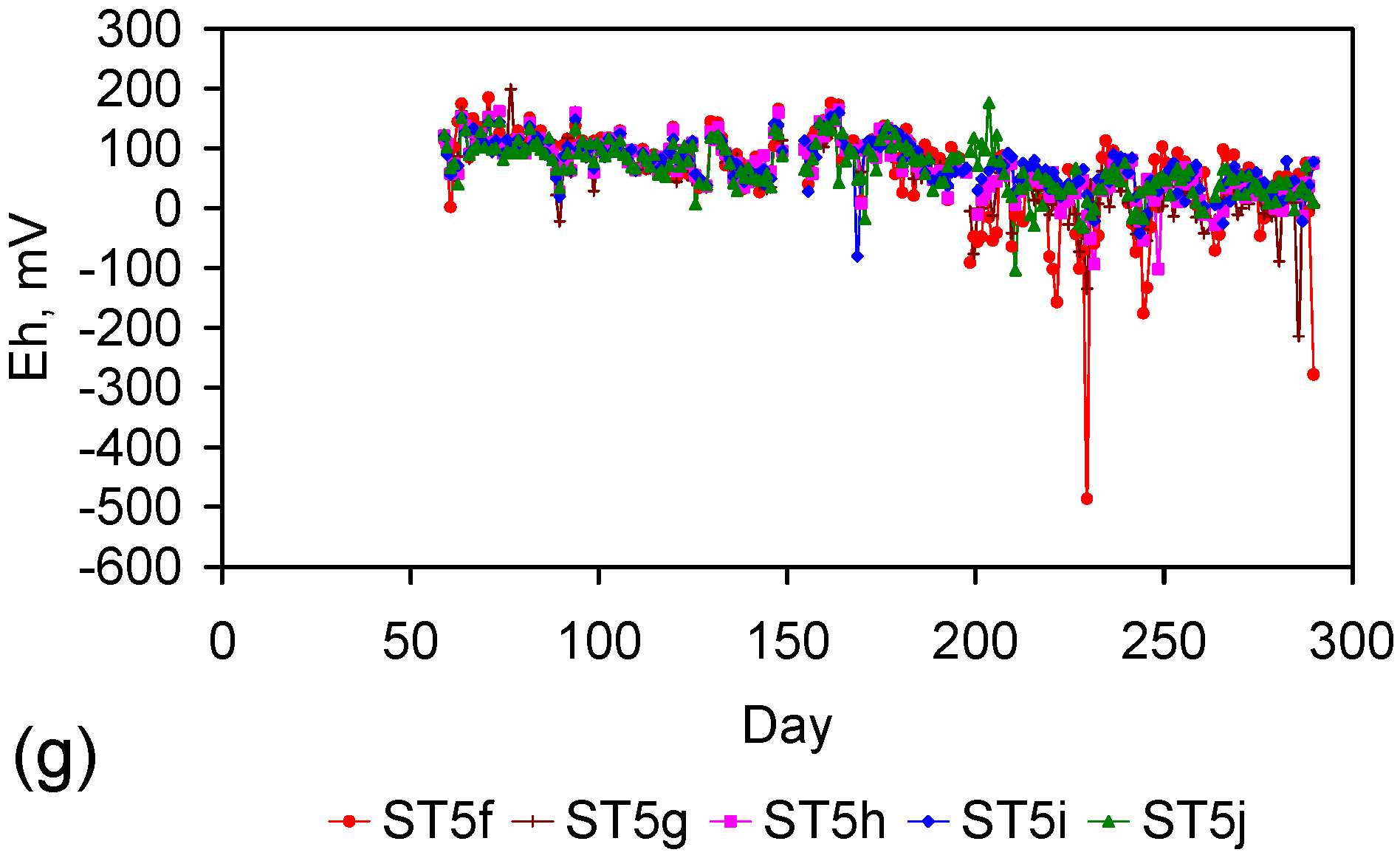
Figure C10.
(a) pH vs. Eh; (b) EC vs. day; (c) pH vs. day; (d) Eh vs. day; (e) NaCl Removed (calculated from EC and residual water volume) vs. day. ZVM TP = copper sheathed pellets (15 mm OD) placed in water at a concentration of ST6a = 15.7 g·L−1; ST6b = 15.1 g·L−1; ST6c = 6.8 g·L−1; ST6d = 5.1 g·L−1. Reactor Size: 2.3 L; Feed Water volume: 2.3 L.


Figure C11.
(a) EC vs. day; (b) Eh vs. day; (c) pH vs. day; (d) pH vs. Eh. AS1 = 44 g·L−1; AS2 = 55 g·L−1; AS3 = 49 g·L−1. Reactor Size: 0.3 L; Feed Water volume: 0.2 L.
Figure C11.
(a) EC vs. day; (b) Eh vs. day; (c) pH vs. day; (d) pH vs. Eh. AS1 = 44 g·L−1; AS2 = 55 g·L−1; AS3 = 49 g·L−1. Reactor Size: 0.3 L; Feed Water volume: 0.2 L.

Figure C12.
(a) EC vs. day; (b) Eh vs. day; (c) pH vs. day; (d) pH vs. Eh; (e) NaCl Removed (calculated from EC and residual water volume) vs. day. ST8a = 37 g·L−1; ST8b = 43 g·L−1; ST8c = 40.4 g·L−1; ST8d = 26 g·L−1; ST8e = 36.5 g·L−1. Reactor Size (ST8a): 0.3 L; Feed Water volume: 0.2 L. Reactor Size (ST8b–ST8d): 2.3 L; Feed Water volume: 2.3 L. Reactor Size (ST8e): 10 L; Feed Water volume: 6.9 L.

Figure C13.
(a) EC vs. day; (b) Eh vs. day; (c) pH vs. day; (d) pH vs. Eh; (e) NaCl Removed (calculated from EC and residual water volume) vs. day. MT1a = 45 g·L−1; MT1b = 43 g·L−1; MT1c = 51.3 g·L−1; MT1d = 30.4 g·L−1. MT1d was successively acidized (using CH2O2) and alkalized (using CaCO3) after Day 200. Reactor Size (MT1a): 0.3 L; Feed Water volume: 0.2 L. Reactor Size (MT1b–MT1d): 2.3 L; Feed Water volume: 2.3 L.
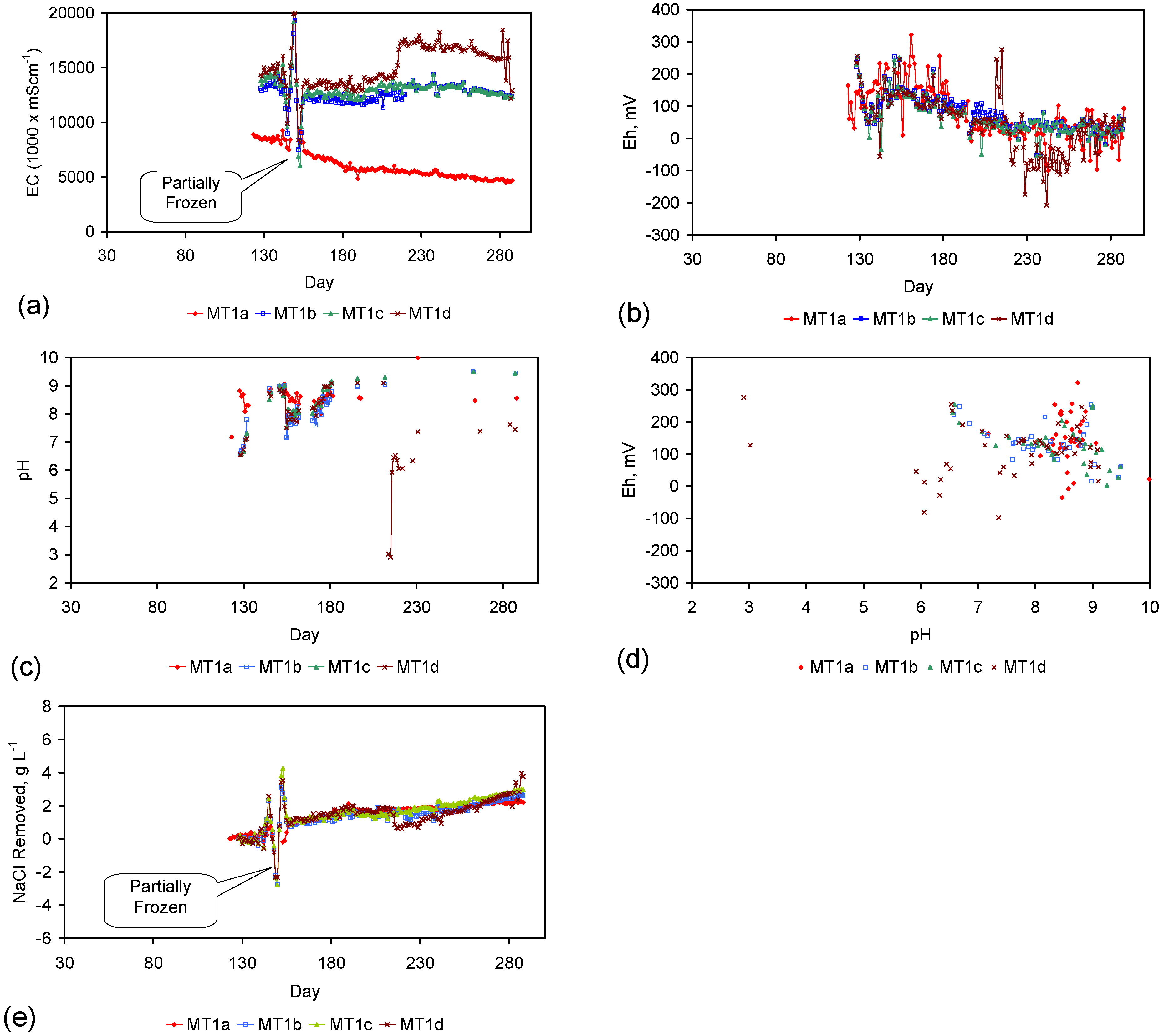
Figure C14.
(a) EC vs. day; (b) Eh vs. day; (c) pH vs. day; (d) pH vs. Eh; (e) NaCl Removed (calculated from EC and residual water volume) vs. day. MT2a = 79.5 g·L−1; MT2b = 121.3 g·L−1; MT2c = 49.5 g·L−1; MT2d = 36.1 g·L−1. Reactor Size (MT2a): 0.3 L; Feed Water volume: 0.2 L. Reactor Size (MT2b–MT2d): 2.3 L; Feed Water volume: 2.3 L.

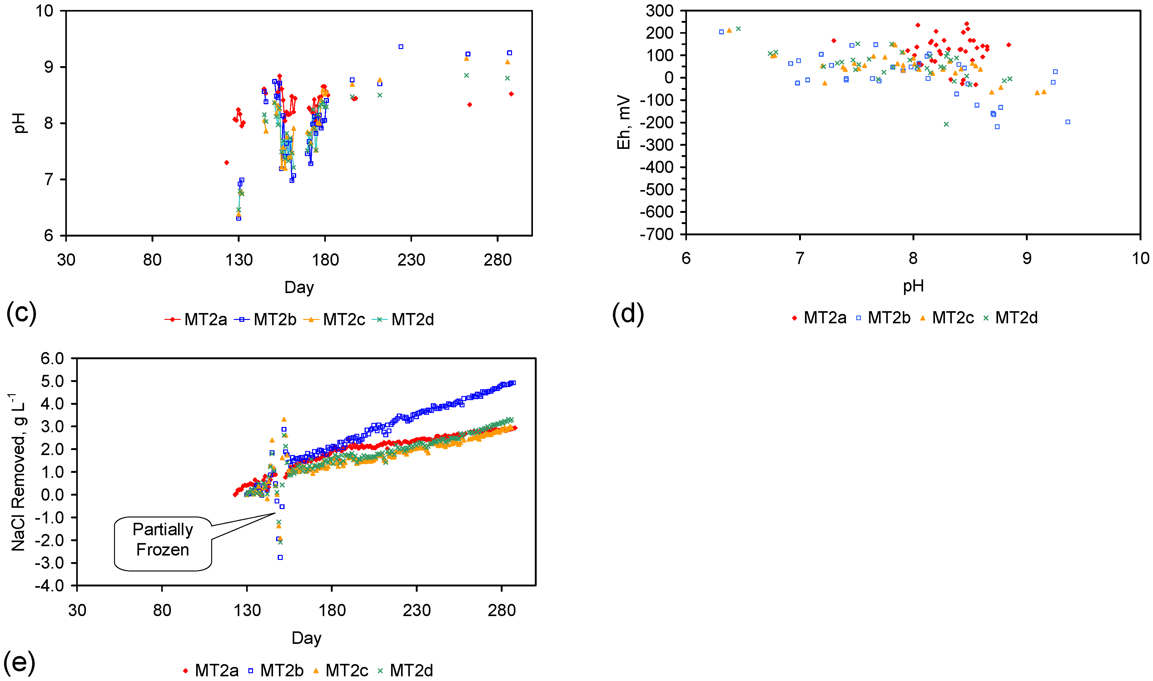
Figure C15.
(a) EC vs. day; (b) Eh vs. day; (c) pH vs. day; (d) pH vs. Eh; (e) NaCl Removed (calculated from EC and residual water volume) vs. day. MT3a = 73.5 g·L−1; MT3b = 62.6 g·L−1; MT3c = 52.6 g·L−1; MT3d = 62.9 g·L−1. Reactor Size (MT3a–MT3c): 2.3 L; Feed Water volume: 2.3 L. Reactor Size (MT3d): 10 L; Feed Water volume: 6.9 L.


Figure C16.
(a) EC vs. day; (b) Eh vs. day; (c) pH vs. day; (d) pH vs. Eh; (e) NaCl Removed (calculated from EC and residual water volume) vs. day. MT4a = 91.3 g·L−1; MT4b = 87.8 g·L−1; MT4c = 91.3 g·L−1; MT4d = 90.1 g·L−1. Reactor Size (MT4a–MT4c): 2.3 L; Feed Water volume: 2.3 L. Reactor Size (MT4d): 10 L; Feed Water volume: 6.9 L.

Figure C17.
(a) EC vs. day; (b) Eh vs. day; (c) pH vs. day; (d) pH vs. Eh. Reactor Size: 0.3 L; Feed Water volume: 0.2 L.
Figure C17.
(a) EC vs. day; (b) Eh vs. day; (c) pH vs. day; (d) pH vs. Eh. Reactor Size: 0.3 L; Feed Water volume: 0.2 L.
Figure C18.
Observed anion and cation removal associated with NaCl removal. (a) nitrates; (b) sulphates; (c) calcium; (d) magnesium; (e) manganese; (f) phosphorous; (g) sulphur; (h) boron; (i) barium; (j) cadmium; (k) cobalt; (l) copper; (m) silicon; (n) strontium; (o) zinc; (p) nickel; (q) arsenic; (r) potassium increases are due to desorption from ZVM TP.


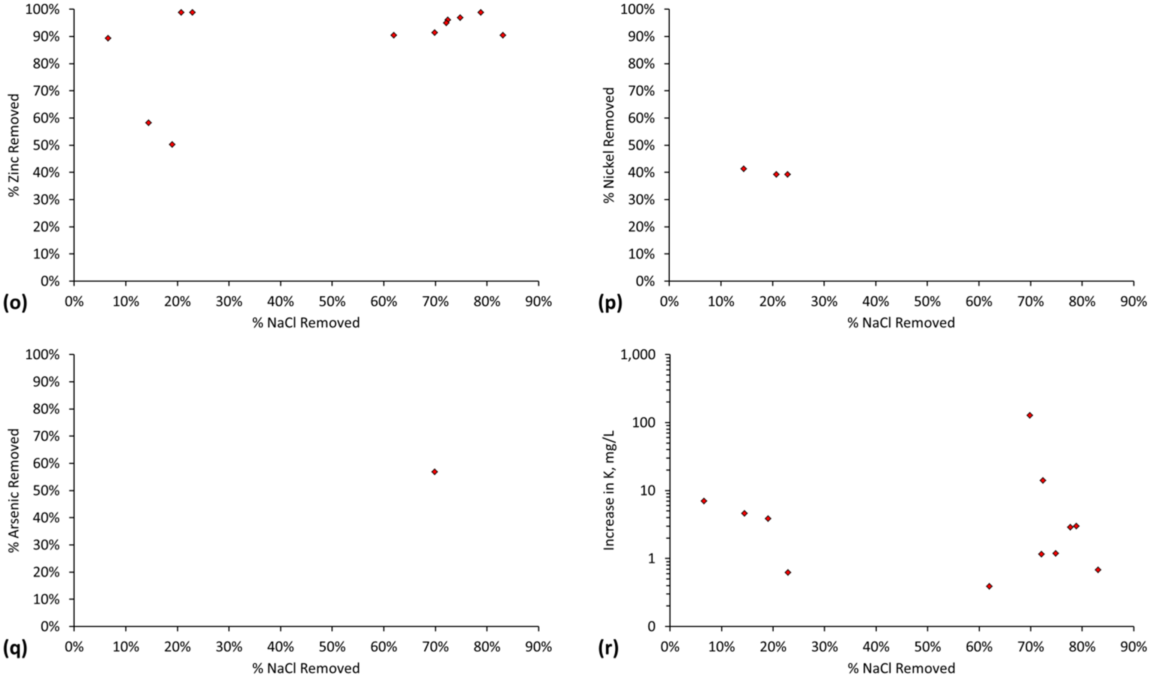
Figure C19.
ZVM TPA Trial E145 Example. Initial Batch Run; Operating Temperature: 13–17 °C; Oxidising Environment: Water volume in the reactor = 0.114 m3; ZVM TP in a cartridge = 1.449 kg; Air flow = 120 L·h−1. (a) Eh vs. time; (b) pH vs. time; (c) pH vs. Eh; (d) Salinity vs. time; (e) Salinity calculated from normalised data vs. salinity calculated from raw data; (f) EC vs. time.
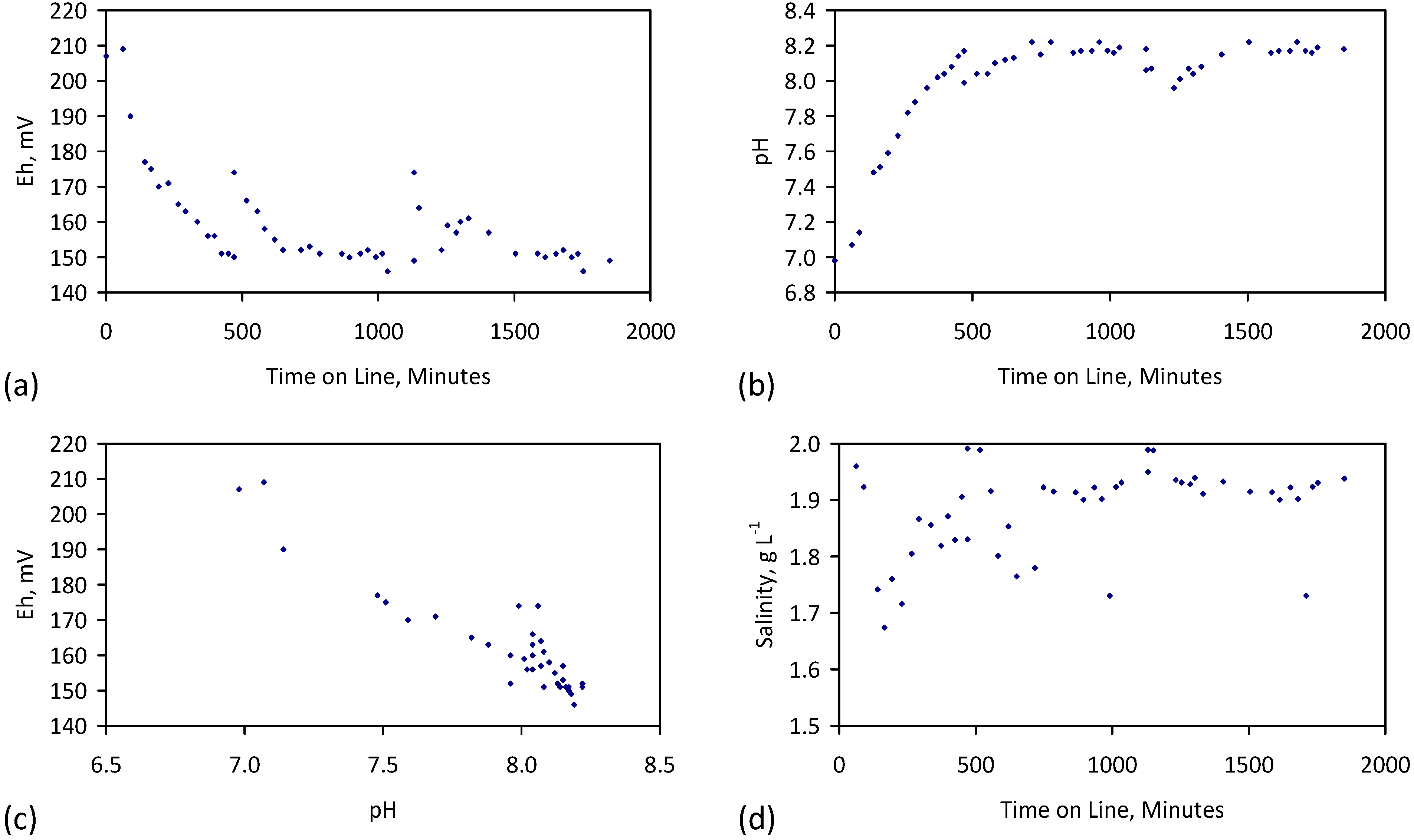

Figure C20.
ZVM TPA Example, Trial E146. Initial Batch Run; Operating Temperature: 17–20 °C; Oxidising Environment: Water volume in the reactor = 0.24 m3; ZVM TP in a cartridge = 0.4 kg. The cartridge (and ZVM TPA) had previously been used in Trial E145. Air flow = 120 L·h−1. (a) Eh vs. time; (b) pH vs. time; (c) pH vs. Eh; (d) Salinity vs. time; (e) Salinity calculated from normalised data vs. salinity calculated from raw data. (f) EC vs. time.

Figure C21.
ZVM TPA example Trial E146. 1st Reuse; Operating Temperature: 15–20 °C; Oxidising Environment: Water volume in the reactor = 0.24 m3; ZVM TPA from Trial E145 in a cartridge = 0.4 kg; Air flow = 120 L·h−1; (a) Eh vs. time; (b) pH vs. time; (c) pH vs. Eh; (d) Salinity vs. time; (e) Salinity calculated from normalised data vs. salinity calculated from raw data; (f) EC vs. time.
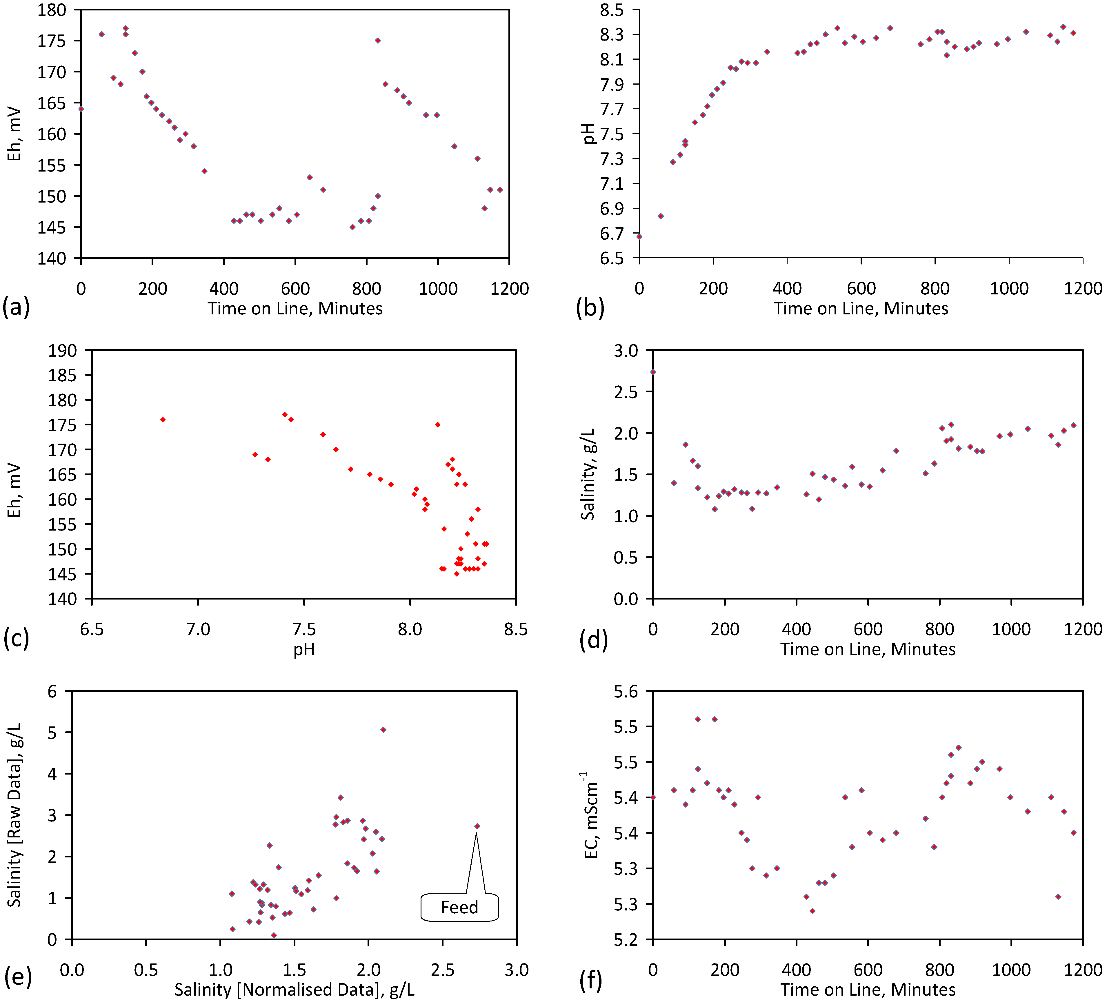
Figure C22.
ZVM TPA example Trial E146. 2nd Reuse; Operating Temperature: 15–22 °C; Oxidising Environment: Water volume in the reactor = 0.24 m3; ZVM TPA from Trial E145 in a cartridge = 0.4 kg; Air flow = 120 L·h−1. (a) Eh vs. time; (b) pH vs. time; (c) pH vs. Eh; (d) Salinity vs. time; (e) Salinity calculated from normalised data vs. salinity calculated from raw data; (f) EC vs. time.
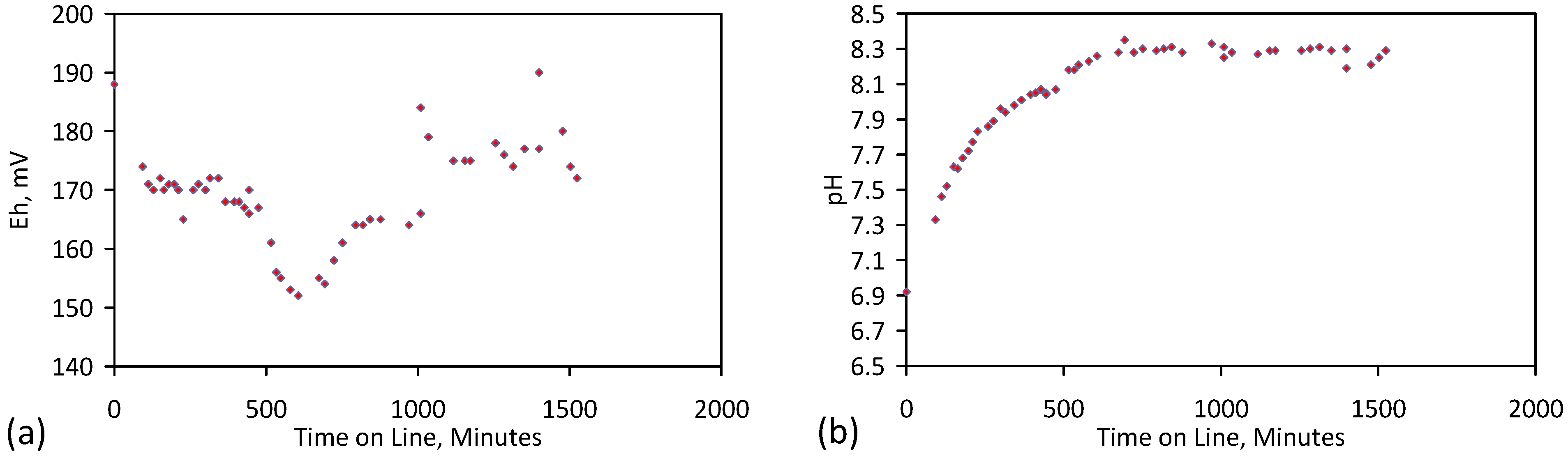
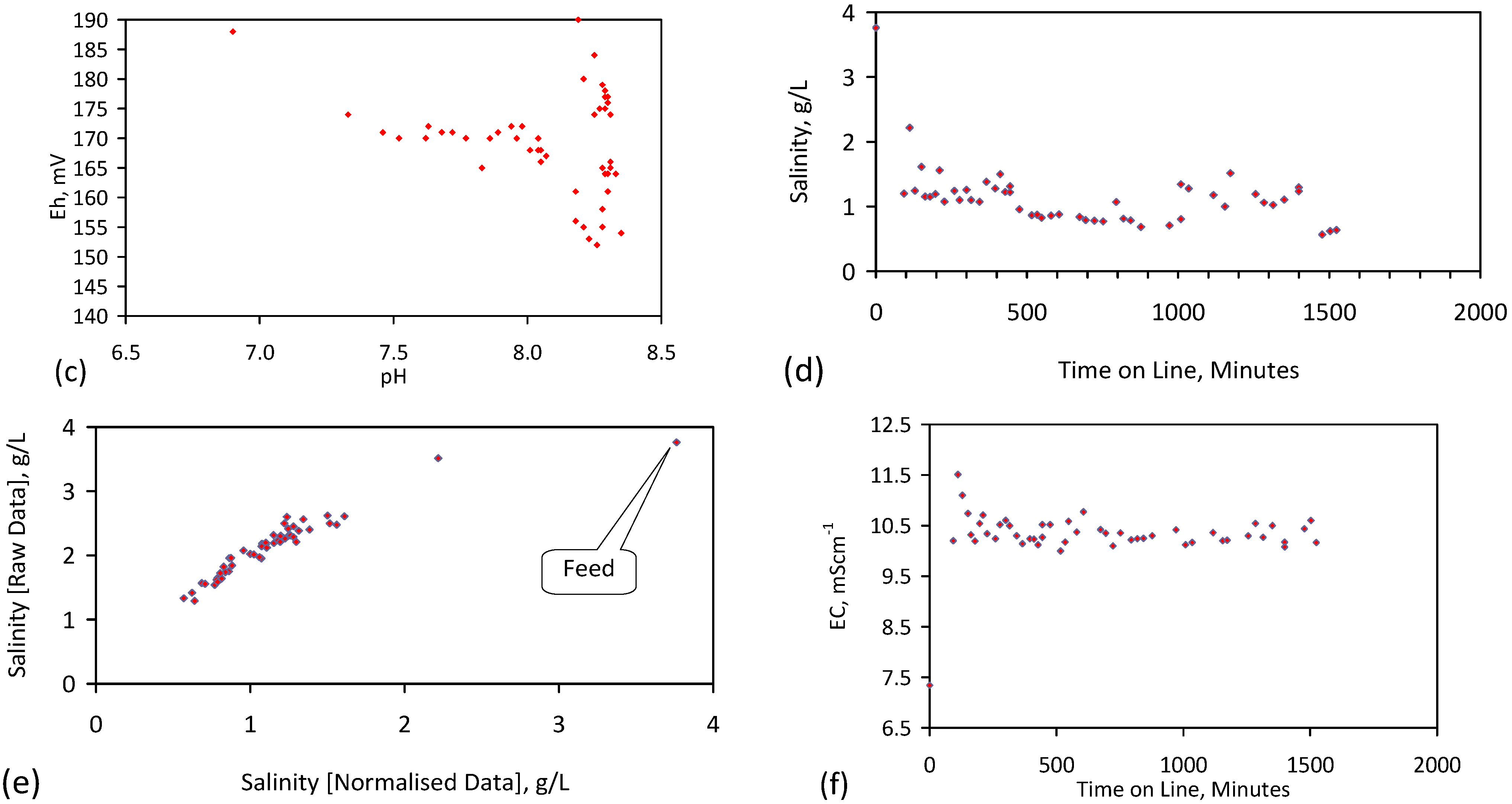
Figure C23.
ZVM TPA example Trial E146. 3rd Reuse; Operating Temperature: 15–21 C; Oxidising Environment: Water volume in the reactor = 0.24 m3; ZVM TPA from Trial E145 in a cartridge = 0.4 kg; Air flow = 120 L·h−1. (a) Eh vs. time; (b) pH vs. time; (c) pH vs. Eh; (d) Salinity vs. time; (e) Salinity calculated from normalised data vs. salinity calculated from raw data; (f) EC vs. time.
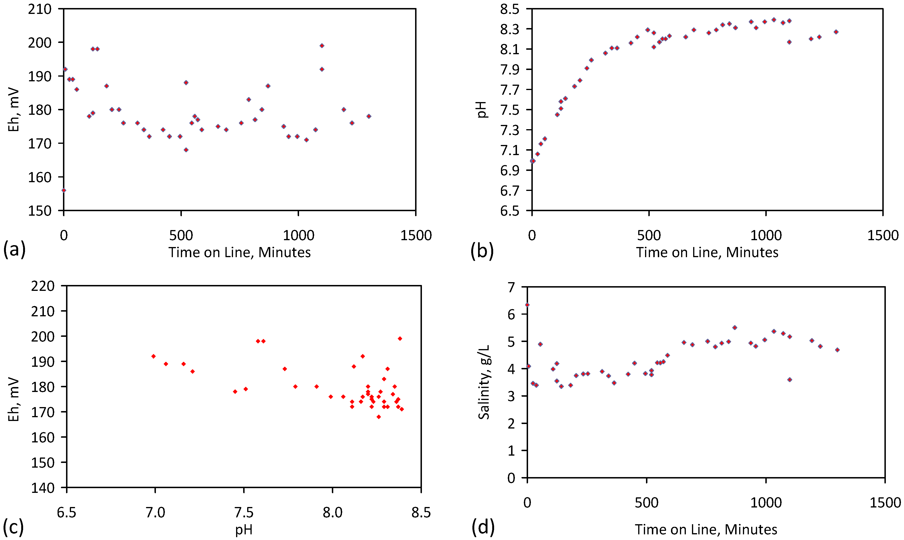
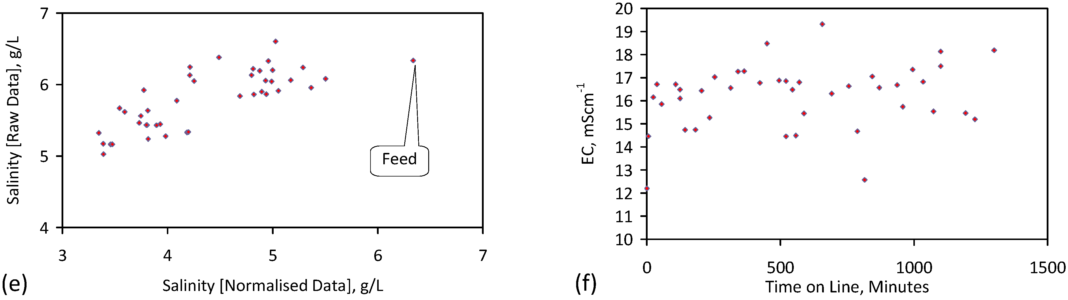
Figure C24.
ZVM TPA example Trial E146. 4th Reuse; Operating Temperature: 15–22 °C; Oxidising Environment: Water volume in the reactor = 0.24 m3; ZVM TPA from Trial E145 in a cartridge = 0.4 kg; Air flow = 120 L·h−1. (a) Eh vs. time; (b) pH vs. time; (c) pH vs. Eh; (d) Salinity vs. time; (e) Salinity calculated from normalised data vs. salinity calculated from raw data; (f) EC vs. time.
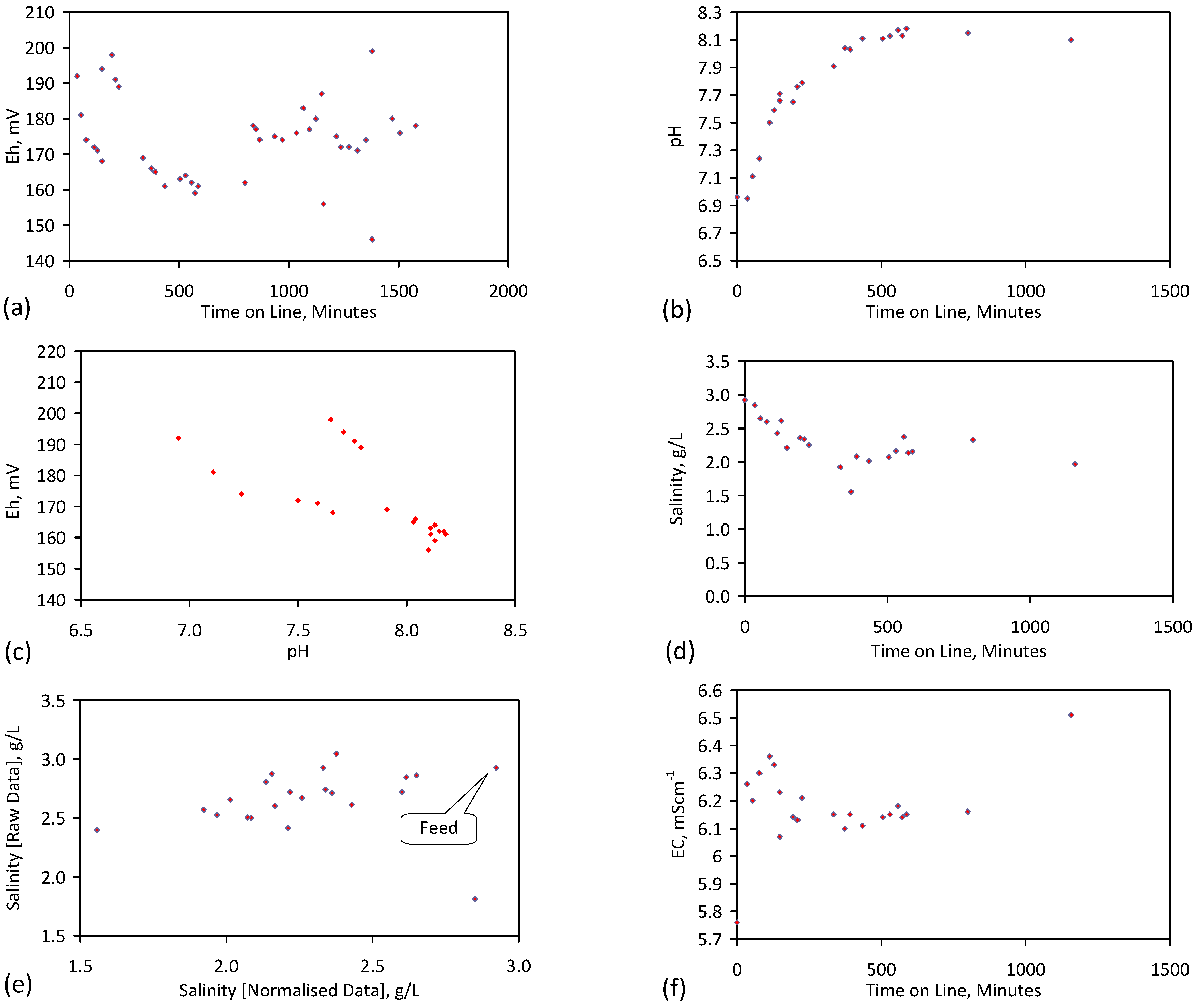
Figure C25.
ZVM TPA example Trial E146. 5th Reuse; Operating Temperature: 17–23 °C; Oxidising Environment: Water volume in the reactor = 0.24 m3; ZVM TPA from Trial E145 in a cartridge = 0.4 kg; Air flow = 120 L·h−1. (a) Eh vs. time; (b) pH vs. time; (c) pH vs. Eh; (d) Salinity vs. time; (e) Salinity calculated from normalised data vs. salinity calculated from raw data; (f) EC vs. time.

Figure C26.
ZVM TPA example Trial E146. 6th Reuse; Operating Temperature: 19–25 °C; Oxidising Environment: Water volume in the reactor = 0.24 m3; ZVM TPA from Trial E145 in a cartridge = 0.4 kg; Air flow = 120 L·h−1. (a) Eh vs. time; (b) pH vs. time; (c) pH vs. Eh; (d) Salinity vs. time; (e) Salinity calculated from normalised data vs. salinity calculated from raw data; (f) EC vs. time.
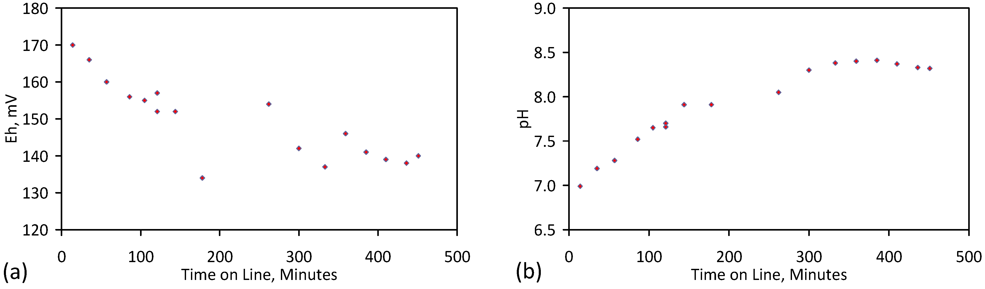

Figure C27.
ZVM TPA example Trial E146. 7th Reuse; Operating Temperature: 18–22 °C; Oxidising Environment: Water volume in the reactor = 0.24 m3; ZVM TPA from Trial E145 in a cartridge = 0.4 kg; Air flow = 120 L·h−1. (a) Eh vs. time; (b) pH vs. time; (c) pH vs. Eh; (d) Salinity vs. time; (e) Salinity calculated from normalised data vs. salinity calculated from raw data; (f) EC vs. time.
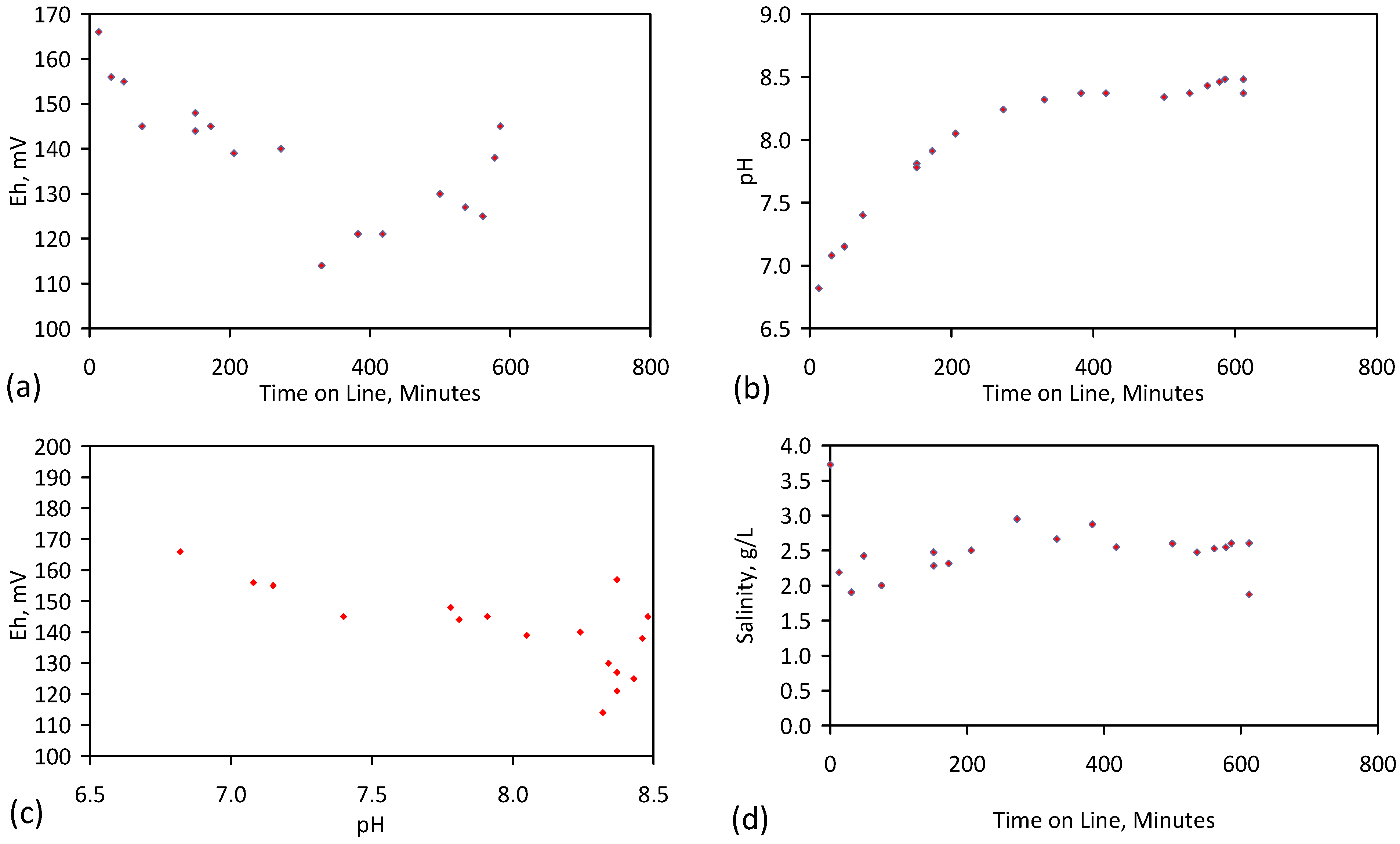
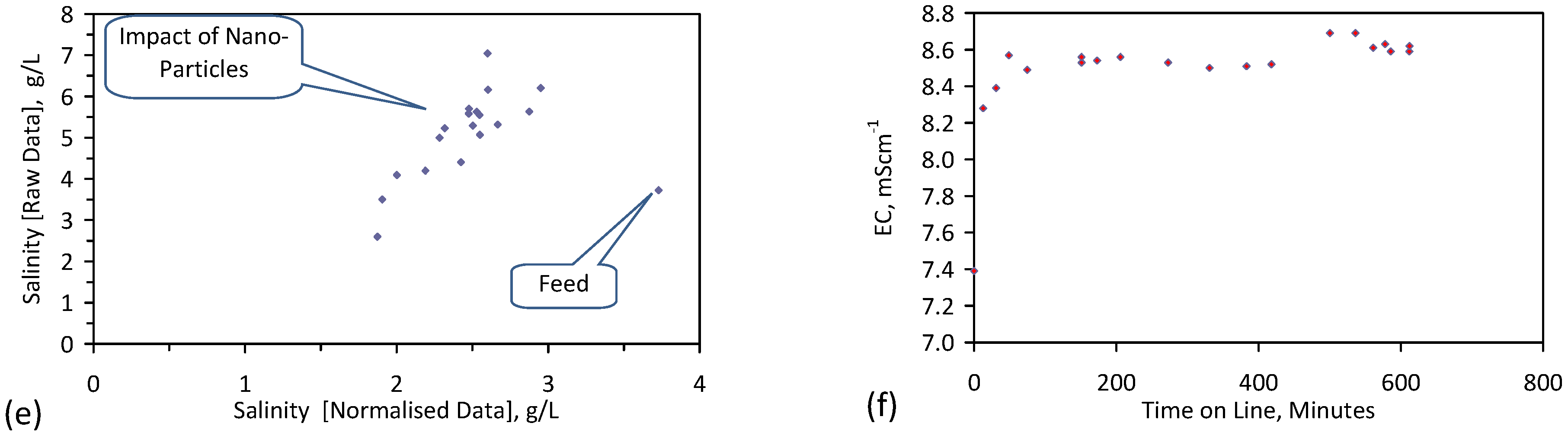
Figure C28.
ZVM TPA example Trial E146. 8th Reuse; Operating Temperature: 15–21 °C; Oxidising Environment: Water volume in the reactor = 0.24 m3; ZVM TPA from Trial E145 in a cartridge = 0.4 kg; Air flow = 120 L·h−1. (a) Eh vs. time; (b) pH vs. time; (c) pH vs. Eh; (d) Salinity vs. time; (e) Salinity calculated from normalised data vs. salinity calculated from raw data; (f) EC vs. time.

Figure C29.
ZVM TPA example Trial E146. 9th Reuse; Operating Temperature: 16–20 °C; Oxidising Environment: Water volume in the reactor = 0.24 m3; ZVM TPA from Trial E145 in a cartridge = 0.4 kg; Air flow = 120 L·h−1. (a) Eh vs. time; (b) pH vs. time; (c) pH vs. Eh; (d) Salinity vs. time; (e) Salinity calculated from normalised data vs. salinity calculated from raw data; (f) EC vs. time.

Figure C30.
ZVM TPA example Trial E146. 10th Reuse; Operating Temperature: 16–21 °C; Oxidising Environment: Water volume in the reactor = 0.24 m3; ZVM TPA from Trial E145 in a cartridge = 0.4 kg; Air flow = 120 L·h−1. (a) Eh vs. time; (b) pH vs. time; (c) pH vs. Eh; (d) Salinity vs. time; (e) Salinity calculated from normalised data vs. salinity calculated from raw data; (f) EC vs. time.


Figure C31.
ZVM TPA example Trial E146. 11th Reuse; Operating Temperature: 15–20 °C; Oxidising Environment: Water volume in the reactor = 0.24 m3; ZVM TPA from Trial E145 in a cartridge = 0.4 kg; Air flow = 120 L·h−1. (a) Eh vs. time; (b) pH vs. time; (c) pH vs. Eh; (d) Salinity vs. time; (e) Salinity calculated from normalised data vs. salinity calculated from raw data; (f) EC vs. time. The rise in absorbance is associated with a rise in EC.
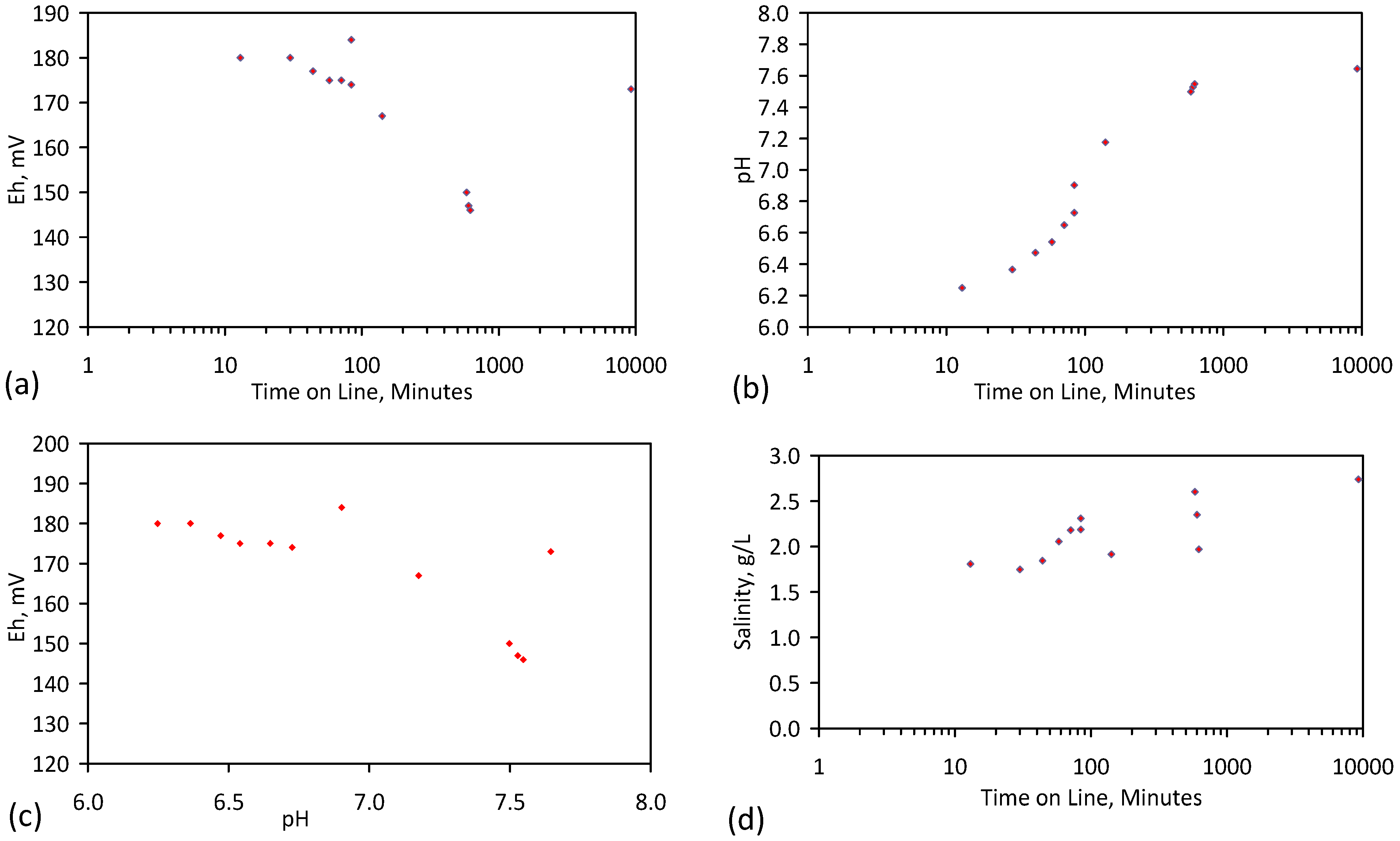

Figure C32.
ZVM TPA example Trial E146. 12th Reuse; Operating Temperature: 14–20 °C; Oxidising Environment: Water volume in the reactor = 0.24 m3; ZVM TPA from Trial E145 in a cartridge = 0.4 kg; Air flow = 120 L·h−1. Acid Oxidising Environment: Water volume in the reactor = 5.5 L; ZVM TP in a cartridge = 0.1 kg; Gas flow (80% N2 + 20% CO2) = 1.8 L·h−1. (a) Eh vs. time; (b) pH vs. time; (c) pH vs. Eh; (d) Salinity vs. time; (e) Salinity calculated from normalised data vs. salinity calculated from raw data; (f) EC vs. time.

Figure C33.
ZVM TPA example Trial E146. 13th Reuse; Operating Temperature: 11–19 °C; Oxidising Environment: Water volume in the reactor = 0.24 m3; ZVM TPA from Trial E145 in a cartridge = 0.4 kg; Air flow = 120 L·h−1. Acid Oxidising Environment: Water volume in the reactor = 5.4 L; ZVM TPA from Trial E144 in a cartridge = 0.4 L; Gas flow (80% N2 + 20% CO2) = 3.3 L·h−1. (a) Eh vs. time; (b) pH vs. time; (c) pH vs. Eh; (d) Salinity vs. time; (e) Salinity calculated from normalised data vs. salinity calculated from raw data; (f) EC vs. time.
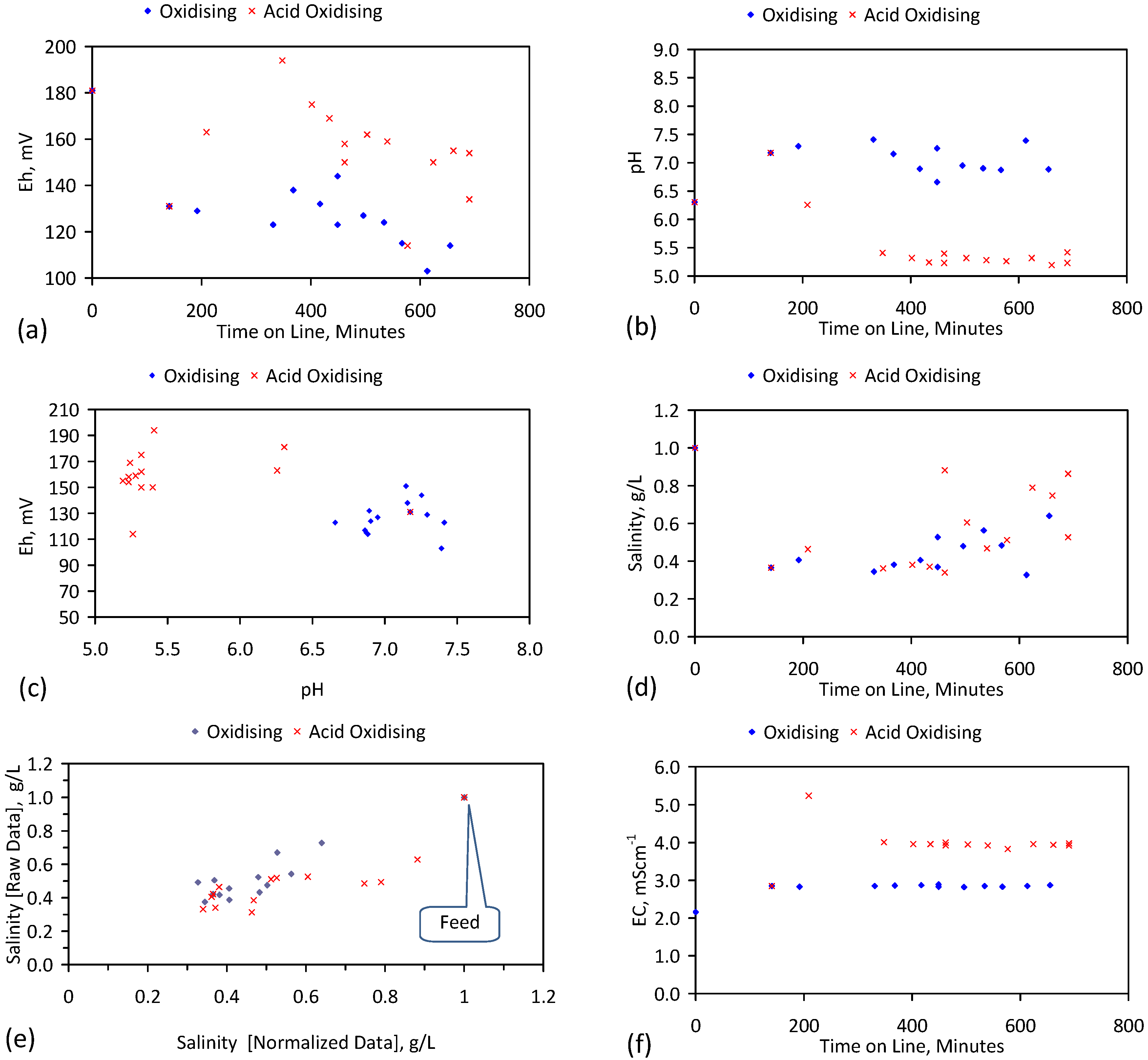
Figure C34.
ZVM TPA example Trial E146. 14th Reuse; Operating Temperature: 12–16 °C; Oxidising Environment: Water volume in the reactor = 0.24 m3; ZVM TPA from Trial E145 in a cartridge = 0.4 kg; Air flow = 120 L·h−1. Acid Oxidising Environment: Water volume in the reactor = 5.4 L; ZVM TPA from Trial E144 in a cartridge = 0.4 L; Gas flow (80% N2 + 20% CO2) = 3.3 L·h−1. (a) Eh vs. time; (b) pH vs. time; (c) pH vs. Eh; (d) Salinity vs. time; (e) Salinity calculated from normalised data vs. salinity calculated from raw data; (f) EC vs. time.


Figure C35.
ZVM TPA example Trial E146. 15th Reuse; Operating Temperature: 16–20 °C; Oxidising Environment: Water volume in the reactor = 0.24 m3; ZVM TPA from Trial E145 in a cartridge = 0.4 kg; Air flow = 120 L·h−1. Acid Oxidising Environment: Water volume in the reactor = 5.4 L; ZVM TPA from Trial E144 in a cartridge = 0.4 L; Gas flow (80% N2 + 20% CO2) = 3.3 L·h−1. (a) Eh vs. time; (b) pH vs. time; (c) pH vs. Eh; (d) Salinity vs. time; (e) Salinity calculated from normalised data vs. salinity calculated from raw data. (f) EC vs. time.
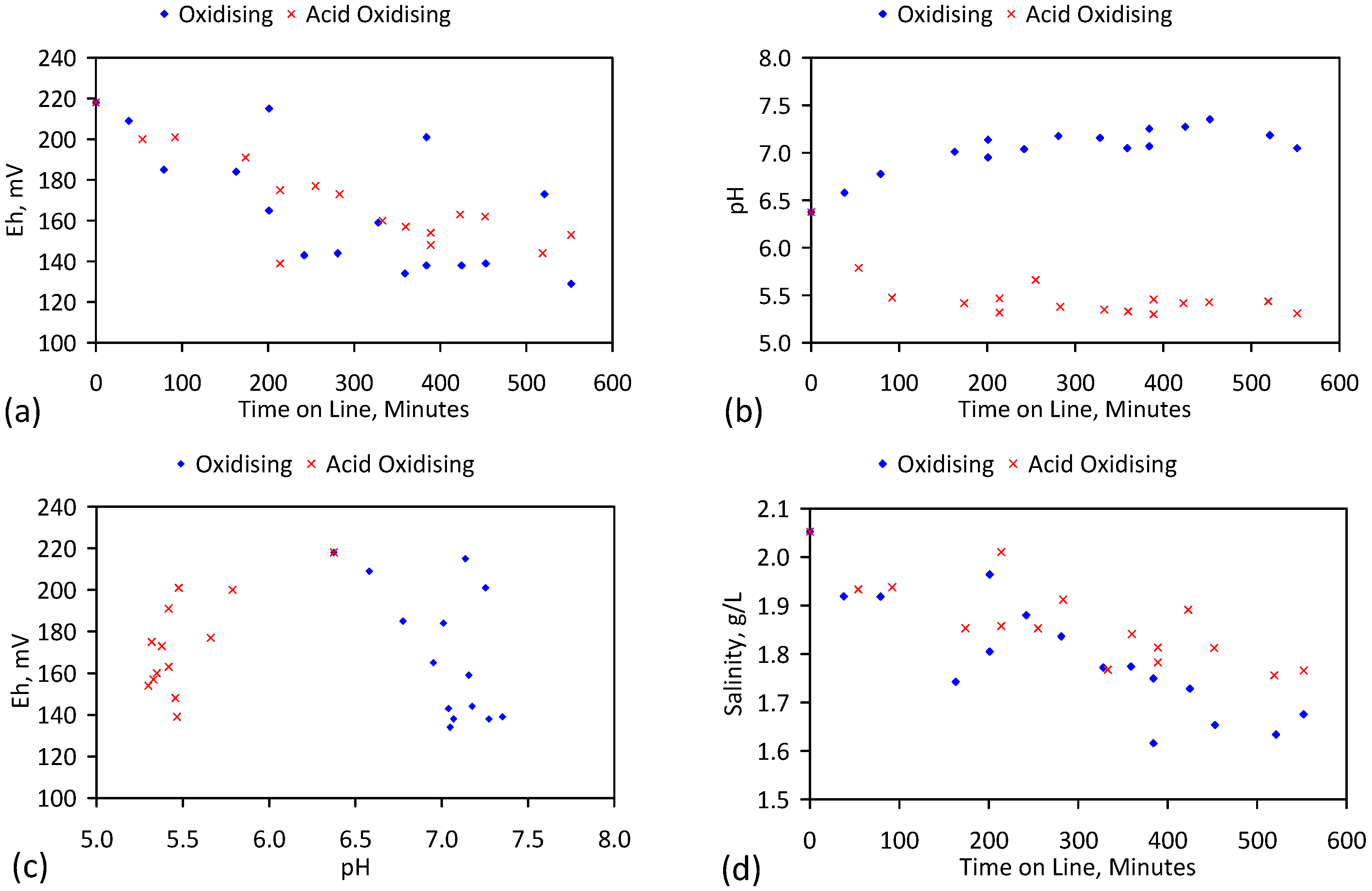
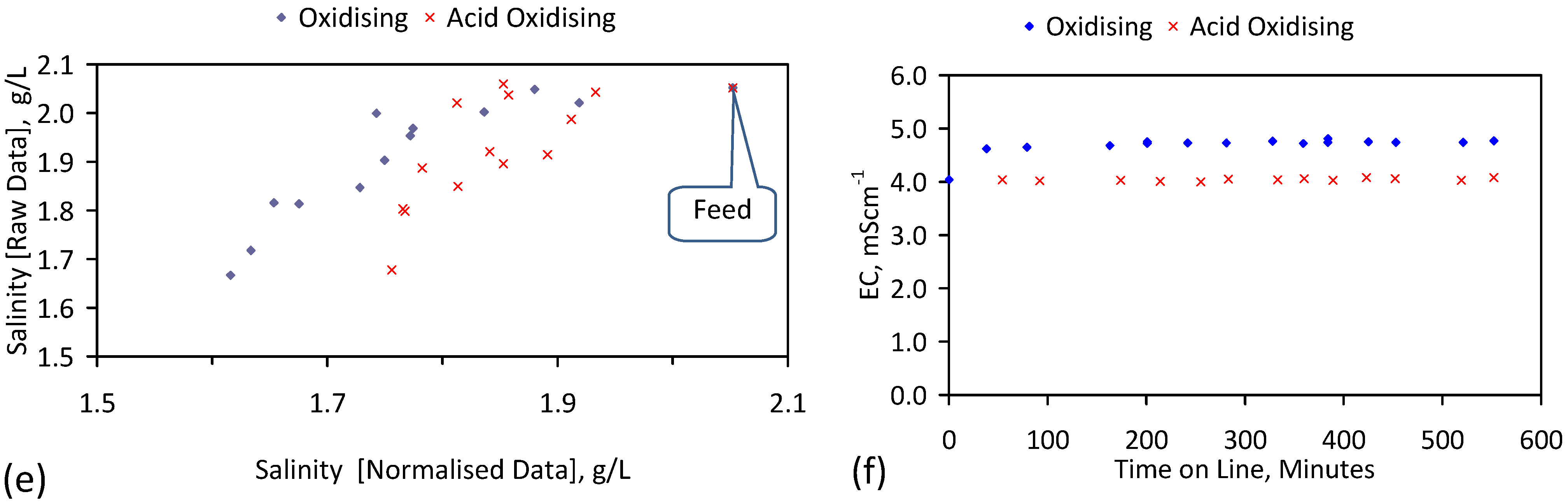
Figure C36.
ZVM TPA example Trial E146]. 16th Reuse; Operating Temperature: 13–20 °C; Oxidising Environment: Water volume in the reactor = 0.24 m3; ZVM TPA from Trial E145 in a cartridge = 0.4 kg; Air flow = 120 L·h−1. Acid Oxidising Environment: Water volume in the reactor = 5.4 L; ZVM TPA from Trial E144 in a cartridge = 0.4 L; Gas flow (80% N2 + 20% CO2) = 3.3 L·h−1. (a) Eh vs. time; (b) pH vs. time; (c) pH vs. Eh; (d) Salinity vs. time; (e) Salinity calculated from normalised data vs. salinity calculated from raw data; (f) EC vs. time.


Figure C37.
Nano-particle UV-Visible spectrograms: (a) Trial E145, 200–900 nm; (b) Trial E145, 200–300 nm; (c) Trial E146, 200–900 nm; (d) Trial E146, 200–300 nm; (e) Trial E146, 1st Reuse, 200–900 nm; (f) Trial E146, 1st Reuse, 200–300 nm; (g) Trial E146, 2nd Reuse, 200–900 nm; (h) Trial E146, 2nd Reuse, 200–300 nm; (i) Trial E146, 3rd Reuse, 200–900 nm; (j) Trial E146, 3rd Reuse, 200–300 nm; (k) Trial E146, 4th Reuse, 200–900 nm; (l) Trial E146, 4th Reuse, 200–300 nm; (m) Trial E146, 5th Reuse, 200–900 nm; (n) Trial E146, 5th Reuse, 200–300 nm; (o) Trial E146, 6th Reuse, 200–900 nm; (p) Trial E146, 6th Reuse, 200–300 nm; (q) Trial E146, 7th Reuse, 200–900 nm; (r) Trial E146, 7th Reuse, 200–300 nm; (s) Trial E146, 8th Reuse, 200–900 nm; (t) Trial E146, 8th Reuse, 200–300 nm; (u) Trial E146, 9th Reuse, 200–900 nm; (v) Trial E146, 9th Reuse, 200–300 nm; (w) Trial E146, 10th Reuse, 200–900 nm; (x) Trial E146, 10th Reuse, 200–300 nm; (y) Trial E146, 11th Reuse, 200–900 nm; (z) Trial E146, 11th Reuse, 200–300 nm; (aa) Trial E146, 12th Reuse, 200–900 nm; (ab) Trial E146, 12th Reuse, 200–300 nm; (ac) Trial E146, 13th Reuse (air feed), 200–900 nm; (ad) Trial E146, 13th Reuse (air feed), 200–300 nm; (ae) Trial E146, 13th Reuse (air and CO2 feed), 200–900 nm; (af) Trial E146, 13th Reuse, (air and CO2 feed), 200–300 nm; (ag) Trial E146, 14th Reuse (air feed), 200–900 nm; (ah) Trial E146, 14th Reuse (air feed), 200–300 nm; (ai) Trial E146, 14th Reuse (air and CO2 feed), 200–900 nm; (aj) Trial E146, 14th Reuse, (air and CO2 feed), 200–300 nm; (ak) Trial E146, 15th Reuse (air feed), 200–900 nm; (al) Trial E146, 15th Reuse (air feed), 200–300 nm; (am) Trial E146, 15th Reuse (air and CO2 feed), 200–900 nm; (an) Trial E146, 15th Reuse, (air and CO2 feed), 200–300 nm; (ao) Trial E146, 16th Reuse (air feed), 200–900 nm; (ap) Trial E146, 16th Reuse (air feed), 200–300 nm; (aq) Trial E146, 16th Reuse (air and CO2 feed), 200–900 nm; (ar) Trial E146, 16th Reuse, (air and CO2 feed), 200–300 nm.


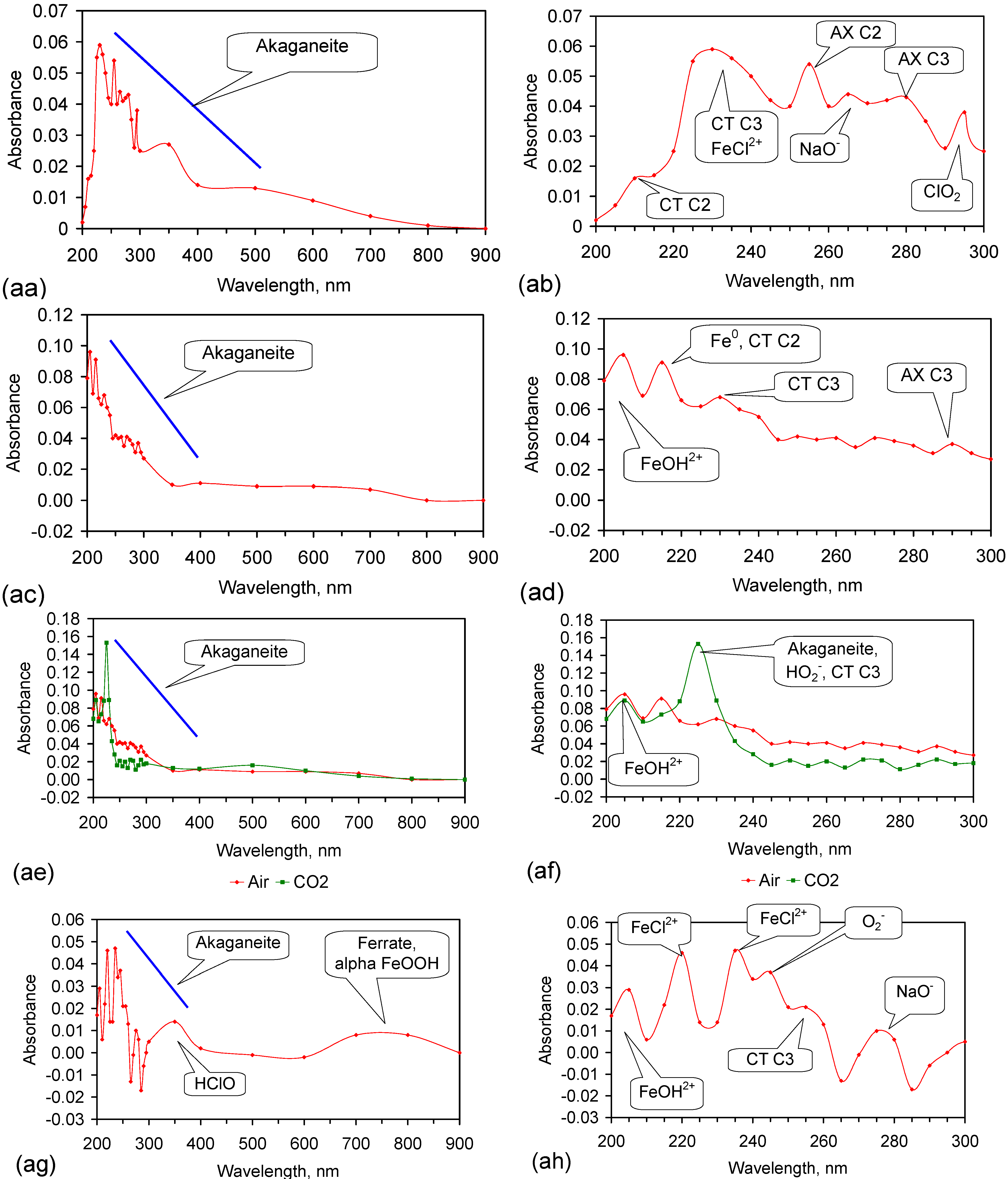


Appendix D. ZVM TP and ZVM TPA Compositions
This Appendix provides details of the ZVM TP and ZVM TPA compositions used in this study (Table D1, Table D2 and Table D3). Details of the ZVM TP control experiment (Figure D1), and details of the salinity decline patterns in ST1a–ST5j (Figure D2, Figure D3, Figure D4, Figure D5 and Figure D6). The surface area of the ZVM particles used to construct the ZVM TP and ZVM TPA was 0.017 m2·g−1 [6].
Table D1.
ZVM TP Manufacturing Processes and Trials; Cu sheathed pellets are 15 mm OD. MDPE sheathed pellets are 20 mm and 25 mm OD. A (g) indicates that the trial group was manufactured in a gaseous environment. All other trial groups were manufactured in an aqueous environment. Trial Group 9 (PS14) was constructed from fine steel wool.
| Trial Group | Manufacturing Process Type | ZVM TP Usage | Trials | Trial Results |
|---|---|---|---|---|
| 1 | B | Particles | PS1–PS4, PS16 | Table 1, Table C1, Table C2, Table C3 and Table C4; Figure C1 |
| 2 | A | Particles | PS5, PS15 | Table 1, Table C1, Table C2, Table C3 and Table C4; Figure C2 |
| 3 | C | Particles | PS8 | Figure C2 |
| 4 | C | Particles | PS9 | Figure C2 |
| 5 | C | Particles | PS10 | Figure C2 |
| 6 | D | Particles | PS11 | Table 1, Table C1, Table C2, Table C3 and Table C4; Figure C3 |
| 7 | D | Particles | PS12 | Figure C3 |
| 8 | D | Particles | PS13 | Figure C3 |
| 9 | A (g) | Cu sheathed pellets | PS14 | Table 1, Table C1, Table C2, Table C3 and Table C4; Figure C3 |
| 10 | D | Container | CSD1a–CSD1d | Table 5 |
| 11 | B | Cu sheathed pellets | AS4–AS6, ST1a–ST5j, ST6a–ST6d | Table 1, Table C1, Table C2, Table C3 and Table C4; Figure C4, Figure C5, Figure C6, Figure C7, Figure C8, Figure C9 and Figure C10 |
| 12 | A | Cu sheathed pellets | AS1–AS3 | Figure C11 |
| 13 | C | Cu sheathed pellets | ST8a | Figure C12 |
| 14 | C | MDPE sheathed pellets | ST8b–ST8e | Table 1, Table C1, Table C2, Table C3 and Table C4; Figure C12 |
| 15 | C | MDPE sheathed pellets | MT1a–MT1d | Table 1, Table C1, Table C2, Table C3 and Table C4; Figure C13 |
| 16 | C | MDPE sheathed pellets | MT2a–MT2d | Table 1, Table C1, Table C2, Table C3 and Table C4; Figure C14 |
| 17 | D | MDPE sheathed pellets | MT3a–MT3d | Table 1, Table C1, Table C2, Table C3 and Table C4; Figure C15 |
| 18 | D | MDPE sheathed pellets | MT4a–MT4d | Table 1, Table C1, Table C2, Table C3 and Table C4; Figure C16 |
| 19 | B | Reused Cu sheathed pellets | ST7a (originally used as ST2d); ST7b (originally used as ST2g); ST7c (originally used as ST3d); ST7d (originally used as ST2f); ST7e (originally used as ST3b); ST7f (originally used as ST3f); | Figure C17 |
Table D2.
ZVM molar compositional ratios used to manufacture ZVM TP. Data in Table 1 from PS7 refer to 50 nm Fe0 (Nanofer Star), as = 20 m2·g−1 [28] (Manufacturing Process Type C; 1 Mole n-Fe0 + 2.14 Moles Al0 + 0.85 Moles Cu0). The Nanofer Star was obtained from Nano Iron s.r.o., Stetanikova 116, Rajhrad, 664 61 Czech Republic.
| Trial Group | Fe | Al | Cu | MnO2 | ZnO | CaCO3 | MgCO3 | K2CO3 | C | CaO |
|---|---|---|---|---|---|---|---|---|---|---|
| 1 | 1 | 0.3950 | 0.040 | 0.006 | - | - | - | - | - | - |
| 2 | 1 | 1.4200 | 0.162 | - | - | - | - | - | - | - |
| 3 | 1 | 0.1100 | - | - | 0.110 | - | - | - | - | - |
| 4 | 1 | 0.1580 | 0.006 | - | - | 0.0900 | 0.060 | 0.017 | 0.16 | - |
| 5 | 1 | 0.5200 | 0.019 | - | - | - | - | - | - | - |
| 6 | 1 | - | - | - | 0.056 | 0.2086 | 0.152 | - | - | - |
| 7 | 1 | 0.8400 | 0.090 | - | 0.068 | 0.0640 | 0.090 | - | - | - |
| 8 | 1 | 0.9700 | 0.040 | - | - | 0.0530 | 0.090 | - | - | 0.07 |
| 9 | 1 | - | - | - | - | - | - | - | - | - |
| 10 | 1 | 0.3200 | - | - | - | - | - | - | - | - |
| 11,19 | 1 | 0.3950 | 0.040 | 0.006 | - | - | - | - | - | - |
| 12 | 1 | 1.4200 | 0.162 | - | - | - | - | - | - | - |
| 13 | 1 | 0.1100 | - | - | 0.110 | - | - | - | - | - |
| 14 | 1 | 0.1100 | - | - | 0.110 | - | - | - | - | - |
| 15 | 1 | 0.1580 | 0.006 | - | - | 0.0900 | 0.060 | 0.017 | 0.16 | - |
| 16 | 1 | 0.5200 | 0.019 | - | - | - | - | - | - | - |
| 17 | 1 | 0.8100 | 0.080 | 0.100 | 0.070 | 0.1500 | 0.100 | - | 0.06 | - |
| 18 | 1 | 0.8200 | 0.040 | - | - | 0.1100 | 0.080 | - | 0.14 | - |
Table D3.
ZVM molar compositional ratios used to manufacture ZVM TPA. K-Feldspar (11.3% K2O + 3.2% NaO + 18.5% Al2O + 65.8% SiO2); Manufacturing Process Type E = dry mixing in air. Al = 5 mm punchings.
| Trial Group | Manufacturing Process Type | ZVM TP Usage | Trials | Trial Results | Cartridge Size, L | Fe, g | K-Feldspar, g | Al, g |
|---|---|---|---|---|---|---|---|---|
| 20 | E | Cartridge | E143a–E143k | Table C5, Table C6, Table C7 and Table C8 | 0.4 | 135 | 97 | - |
| 21 | E | Cartridge | E144a–E144f | Table C9, Table C10, Table C11 and Table C12 | 0.4 | 51 | 90 | 38 |
| 22 | E | Cartridge | E145 | Figure C18 | 2.0 | 449 | 1000 | - |
| 23 | E | Cartridge | E146a–E146p | Table C13, Figure C19, Figure C20, Figure C21, Figure C22, Figure C23, Figure C24, Figure C25, Figure C26, Figure C27, Figure C28, Figure C29, Figure C30, Figure C31, Figure C32, Figure C33, Figure C34, Figure C35, Figure C36 and Figure C37 | 0.4 | 124 | 276 | - |
Figure D1.
(a) Eh vs. day; (b) pH vs. day; (c) pH vs. EC; (d) Eh vs. EC; (e) pH vs. EC; (f) EC vs. day. ZVM TP = particulate material placed in water at a concentration of PS1 = 30 g·L−1; PS1C = 20 g·L−1. Reactor Size: 0.3 L; Feed Water volume: 0.2 L.
Figure D1.
(a) Eh vs. day; (b) pH vs. day; (c) pH vs. EC; (d) Eh vs. EC; (e) pH vs. EC; (f) EC vs. day. ZVM TP = particulate material placed in water at a concentration of PS1 = 30 g·L−1; PS1C = 20 g·L−1. Reactor Size: 0.3 L; Feed Water volume: 0.2 L.

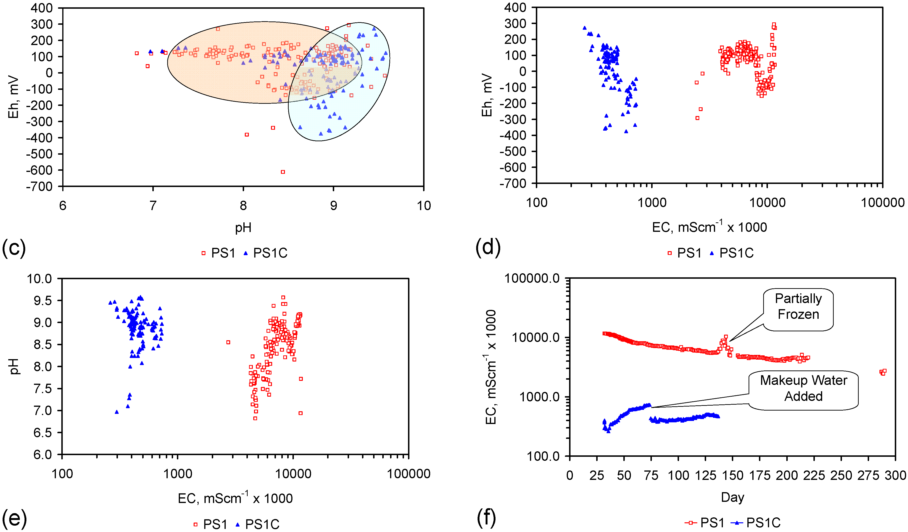
Figure D2.
Feed Water EC = 15.200 mS·cm−1. (a) S1:T1; D = 0.0087; R2 = 0.9941; Z = 18.3; Cu = 36.7; (b) S1:T2; D = 0.0075; R2 = 0.993; Z = 23.1; Cu = 31.9; (c) S1:T3; D = 0.0074; R2 = 0.9912; Z = 25.3; Cu = 44.7; (d) S1:T4; R2 = 0.9937; D = 0.0071; Z = 26.7; Cu = 38.3; (e) S1:T5; D = 0.0071; R2 = 0.9891; Z = 21.7; Cu = 38.3; (f) S1:T6; D = 0.0069; R2 = 0.9938; Z = 28.3; Cu = 36.7; (g) S1:T7; D = 0.0068; R2 = 0.9938; Z = 31.9; Cu = 32.0; (h) S1:T8; D = 0.0074; R2 = 0.9935; Z = 30.1; Cu = 30.1; (i) S1:T9; D = 0.0069; R2 = 0.9938; Z = 23.3; Cu = 36.7; (j) S1:T10; D = 0.0066; R2 = 0.9925; Z = 25.1; Cu = 43.1. Vertical blue-dashed line represents start of the freezing event (indicated by ice formation). D = Exponential Constant D; R2 = Exponential coefficient of determination; Z = ZVM g·L−1; Cu = Cu0 pellet shell weight g·L−1. Trials commenced on Day 59. T1–T10 = Trial numbers. Data extracted from a larger data set in Figure C5.


Figure D3.
Feed Water EC = 17.660 mS·cm−1. (a) S2:T1; D = 0.0066; R2 = 0.9321; Z = 28.5; Cu = 41.5; (b) S2:T2; D = 0.0067; R2 = 0.9188; Z = 30.0; Cu = 40.0; (c) S2:T3; D = 0.0066; R2 = 0.9246; Z = 25.0; Cu = 35.0; (d) S2:T4; D = 0.0070; R2 = 0.9916; Z = 25.0; Cu = 35.0; (e) S2:T5; D = 0.0069; R2 = 0.9925; Z = 33.5; Cu = 41.5; (f) S2:T6; D = 0.0065; R2 = 0.994; Z = 26.5; Cu = 38.5; (g) S2:T7; D = 0.0055; R2 = 0.6045; Z = 26.5; Cu = 38.5; (h) S2:T8; D = 0.0066; R2 = 0.9902; Z = 23.5; Cu = 36.5; (i) S2:T9; D = 0.0064; R2 = 0.9896; Z = 26.5; Cu = 38.5; (j) S2:T10; D = 0.0063; R2 = 0.9091; Z = 33.5; Cu = 41.5. Vertical blue-dashed line represents start of the freezing event (indicated by ice formation). D = Exponential Constant D; R2 = Exponential coefficient of determination; Z = ZVM g·L−1; Cu = Cu0 pellet shell weight g·L−1. Trials commenced on Day 59. T1–T10 = Trial numbers. Data extracted from a larger data set in Figure C6.


Figure D4.
Feed Water EC = 18.480 mS·cm−1. (a) S3:T1; D = 0.0063; R2 = 0.9899; Z = 32.0; Cu = 43.0; (b) S3:T2; D = 0.0061; R2 = 0.9888; Z = 25.0; Cu = 35.0; (c) S3:T3; D = 0.0060; R2 = 0.9896; Z = 30.0; Cu = 40.0; (d) S3:T4; D = 0.0109; R2 = 0.9158; Z = 30.0; Cu = 40.0; (e) S3:T5; D = 0.0062; R2 = 0.9881; Z = 26.5; Cu = 33.5; (f) S3:T6; D = 0.0064; R2 = 0.9875; Z = 57.5; Cu = 92.5; (g) S3:T7; D = 0.0063; R2 = 0.9888; Z = 82.5; Cu = 92.5; (h) S3:T8; D = 0.0060; R2 = 0.9907; Z = 65.0; Cu = 79.5; (i) S3:T9; D = 0.0061; R2 = 0.9879; Z = 72.0; Cu = 83.0; (j) S3:T10; D = 0.0059; R2 = 0.9876; Z = 66.5; Cu = 78.0. Vertical blue-dashed line represents start of the freezing event (indicated by ice formation). D = Exponential Constant D; R2 = Exponential coefficient of determination; Z = ZVM g·L−1; Cu = Cu0 pellet shell weight g·L−1. Trials commenced on Day 59. T1–T10 = Trial numbers. Data extracted from a larger data set in Figure C7.
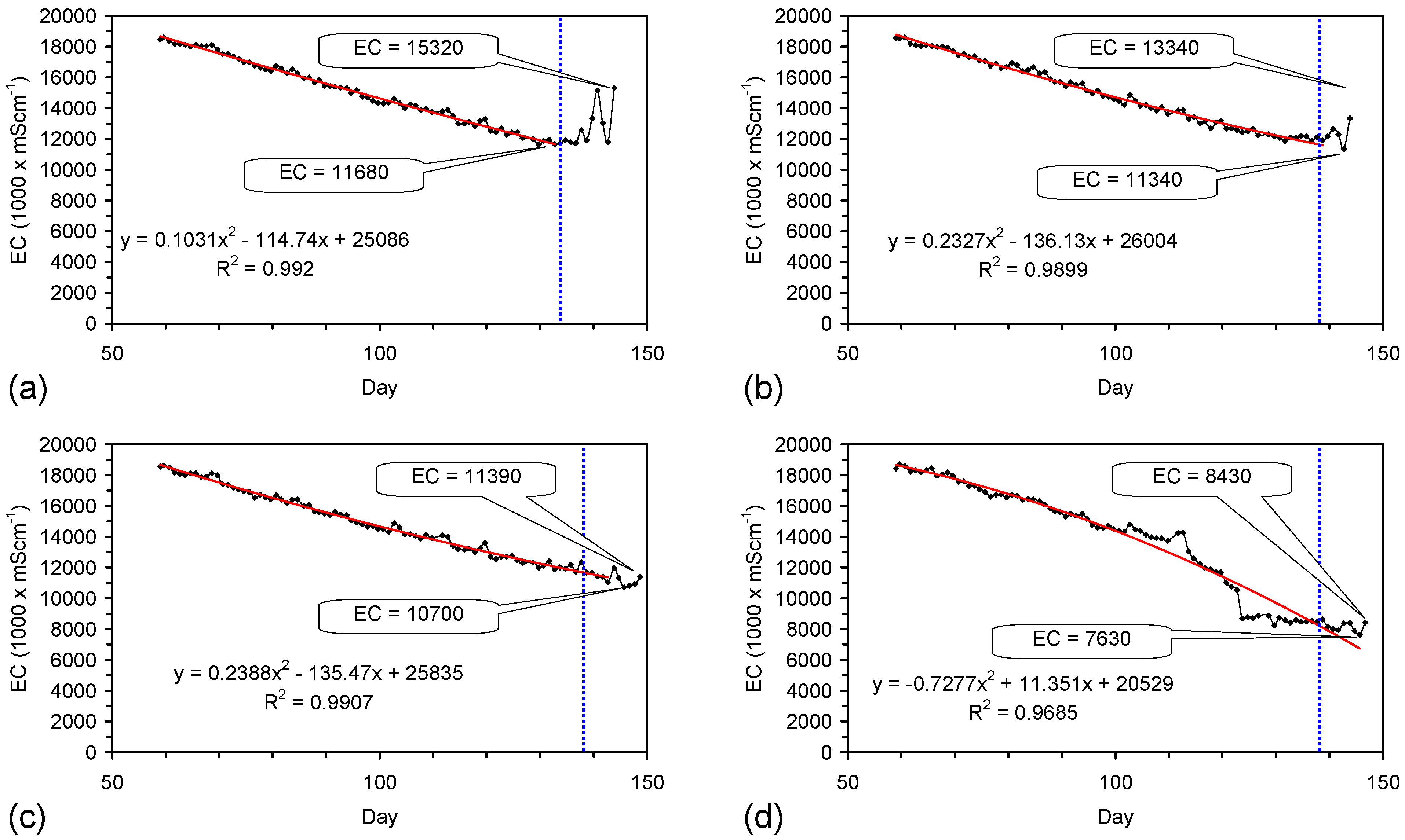

Figure D5.
Feed Water EC = 16.960 mS·cm−1. (a) S4:T1; D = 0.0055; R2 = 0.9832; Z = 50.0; Cu = 80.0; (b) S4:T2; D = 0.0058; R2 = 0.986; Z = 55.5; Cu = 79.5; (c) S4:T3; D = 0.0055; R2 = 0.9832; Z = 50.0; Cu = 75.0; (d) S4:T4; D = 0.0054; R2 = 0.9859; Z = 63.5; Cu = 46.2; (e) S4:T5; D = 0.0053; R2 = 0.9835; Z = 87.5; Cu = 52.5; (f) S4:T6; D = 0.0053; R2 = 0.9846; Z = 44.0; Cu = 55.5; (g) S4:T7; D = 0.0053; R2 = 0.9824; Z = 49.0; Cu = 46.0; (h) S4:T8; D = 0.0055; R2 = 0.9852; Z = 66.5; Cu = 73.5; (i) S4:T9; D = 0.0052; R2 = 0.9804; Z = 36.0; Cu = 59.0; (j) S4:T10; D = 0.0052; R2 = 0.9839; Z = 44.5; Cu = 65.5. Vertical blue-dashed line represents start of the freezing event (indicated by ice formation). D = Exponential Constant D; R2 = Exponential coefficient of determination; Z = ZVM g·L−1; Cu = Cu0 pellet shell weight g·L−1. Trials commenced on Day 59. T1–T10 = Trial numbers. Data extracted from a larger data set in Figure C8.


Figure D6.
Feed Water EC = 17.890 mS·cm−1. (a) S5:T1; D = 0.0054; R2 = 0.9867; Z = 64.0; Cu = 86.0; (b) S5:T2; D = 0.0051; R2 = 0.9819; Z = 47.5; Cu = 57.5; (c) S5:T3; D = 0.0053; R2 = 0.9837; Z = 48.0; Cu = 72.0; (d) S5:T4; D = 0.0051; R2 = 0.9825; Z = 62.5; Cu = 97.5; (e) S5:T5; D = 0.0048; R2 = 0.9775; Z = 94.0; Cu = 130.5; (f) S5:T6; D = 0.0049; R2 = 0.9737; Z = 47.5; Cu = 92.5; (g) S5:T7; D = 0.0042; R2 = 0.7628; Z = 38.0; Cu = 102.0; (h) S5:T8; D = 0.0044; R2 = 0.7484; Z = 46.0; Cu = 94.0; (i) S5:T9; D = 0.0043; R2 = 0.7532; Z = 39.5; Cu = 95.5; (j) S5:T10; D = 0.0042; R2 = 0.7373; Z = 72.5; Cu = 57.5. Vertical blue-dashed line represents start of the freezing event (indicated by ice formation). D = Exponential Constant D; R2 = Exponential coefficient of determination; Z = ZVM g·L−1; Cu = Cu0 pellet shell weight g·L−1. Trials commenced on Day 59. T1–T10 = Trial numbers. Data extracted from a larger data set in Figure C9.

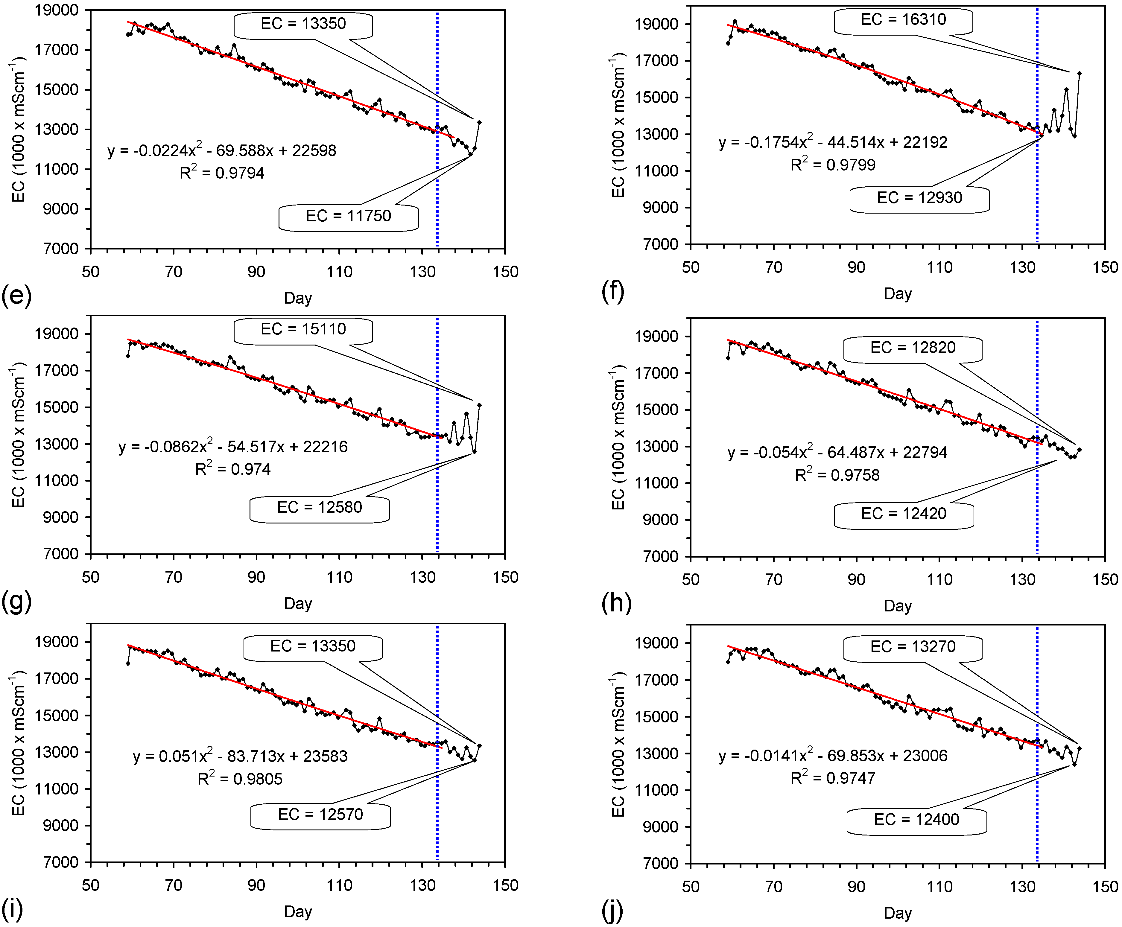
Appendix E. Interpretation of Salinity
Salinity can be measured by directly measuring Cl− ion concentrations in a laboratory, e.g., [21,25], Table C1, or can be measured using calibrated electrical conductivity (EC) [27], or UV-visible spectrometry [215,216] equipment.
Standard salinity calibration analyses assume that the water contains two components: H2O + NaCl [27,215,216]. These analyses assume in a two component system that EC (and absorbance) decrease as the water salinity decreases [27,215,216].
Dissolution of ZVM to form Fen+ ions (and entrained ZVM particles) will both increase EC and absorbance. If the water also contains other components which are removed by the ZVM, then decreases in EC or absorbance may also reflect their removal [27].
The salinity assessment methodology [27,215,216] is extended in this study (incorporating examples using ZVM TPA, when appropriate) as follows:
- (1)
- Assessment of salinity using UV-visible spectrometry
- (a)
- Determination of control samples and salinity using UV-visible spectrometry, when nano-particles are absent;
- (b)
- Determination of salinity when nano-particle formation results in the product water absorbance being greater than the feed water absorbance, and the nano-particles can be removed by settlement;
- (c)
- Determination of salinity when nano-particle formation results in the product water absorbance being less than the feed water absorbance during desalination;
- (2)
- Assessment of salinity using EC
- (a)
- Determination of control samples and salinity using EC, when nano-particles are absent;
- (b)
- Determination of salinity when EC shows an initial rise due to nano-particle formation followed by a decline during desalination;
- (c)
- Determination of salinity removed when the water volume reduces during desalination;
- (3)
- Assessment of salinity using UV-visible spectrometry and EC
- (a)
- Determination of salinity when nano-particle formation results in absorbance increasing with time, while EC initially rises before remaining stable at an elevated level.
E1. Assessment of Product Water Salinity Using UV-Visible Spectrophotometry
There is a relationship between wavelength, absorbance and ion concentration, for most ions and ion adducts (including NaCl [215,216], ClxOy [217,218,219,220], Cl2− [220], ClxOyHz [218], OxH [221,222,223,224,225], Oxn− [225], FeOOH [93,226], Fe(OH)x [226], n-Fe0 [227]). Absorbance increases (or decreases), at specific wavelengths, as the ion concentration increases [228]. Nano-particles of akaganeite (beta-FeOOH) can accrete in multi-layered polyionic layers [90]. The average number of accreting layers can be assessed from the absorbance at a wavelength of 225 nm relative to a normalised base layer [90].
The absorbance can be measured relative to a fresh water standard (or another standard), or can be normalized (by setting absorbance at a reference wavelength (in the range 600–1000 nm) to zero) [228].
In this study a control set of water samples was constructed by dissolving halite (NaCl) in water. A total of 43 control water samples were created, where each 2.3 L sample had a different salinity. This data set formed the basis for the assessment of salinity in the product waters during desalination using ZVM TPA (Figure C19, Figure C20, Figure C21, Figure C22, Figure C23, Figure C24, Figure C25, Figure C26, Figure C27, Figure C28, Figure C29, Figure C30, Figure C31, Figure C32, Figure C33, Figure C34, Figure C35 and Figure C36).
The standard wavelength scan recorded absorbance at 5 nm intervals between 200 and 300 nm, absorbance at 350 nm, and absorbance at 100 nm intervals between 400 and 900 nm.
E1.1. Equations Used in the Assessment of Salinity: Control Samples
Absorbance vs. wavelength was calculated for 43 saline control water samples relative to the freshwater standard over the spectral range 200–900 nm (e.g., Figure E1a). All raw spectra were normalized [228] to provide an absorbance value at 900 nm of zero. The normalized data was also corrected for changes in absorbance associated with differences in the optical properties of the quartz cuvette used for the freshwater standard and the saline control water samples [228]. The effect of this normalisation correction [228] is illustrated in Figure E1b.
Figure E1.
Absorbance (relative to reference freshwater control sample) vs. wavelength for different concentrations of halite (g·L−1). (a) Raw control data set, absorbance relative to freshwater; (b) Normalized control data set; (c) Example Product Water after 7.5 h: Raw data, absorbance relative to freshwater. Assessed Salinity of settled product water: Average = 1.63 g·L−1; Standard deviation = 0.41 g·L−1, n = 27; Feed water salinity = 2.467 g·L−1; (d) Example Product Water after 7.5 h: Normalised data [absorbance relative to freshwater] following normalisation to 900 nm. Salinity of settled product water: Average = 0.71 g·L−1; Standard deviation = 0.833 g·L−1, n = 27. Feed water salinity = 2.467 g·L−1; Settlement period = 18.5 h; Water volume treated = 240 L.

The normalised absorbance at 27 different wavelengths (200–800 nm) was cross plotted against measured salinity. 27 calibration regression equations (one for each wavelength measurement), which relate absorbance to salinity at the specific wavelength, were calculated using the trend line function in MS Excel 2010 (Table E1). Each regression calibration equation, for each wavelength, is based on the 43 measured calibration data points.
Table E1.
Equations used to calculate salinity. Calibrated using Cheshire Halite. Valid Range = 0 to 22 gNaCl·L−1. Applicability: two component system only, water + dissolved halite. xraw = raw absorbance value at the measured wavelength of the partially desalinated water. xinitial = the raw absorbance value at the measured wavelength of the feed water. x = the normalized absorbance value at the measured wavelength of the partially desalinated water. This is calculated as x = [xraw (at a specific wavelength)] − [xraw (at a wavelength of 900 nm)]. R = the initial salinity of the feed water, g·L−1. Absorbance is referenced to the freshwater (0 g NaCL L-1) control sample.
| Wavelength, nm | Normalized Absorbance | Raw Absorbance |
|---|---|---|
| Salinity, g·L−1 | Salinity, g·L−1 | |
| 200 | Salinity, g·L−1 = 766.28x2 − 3.2388x + 1.8149 | Salinity, g·L−1 = [xraw/xinitial]·R |
| 205 | Salinity, g·L−1 = 636.34x2 − 10.996x + 1.8025 | Salinity, g·L−1 = [xraw/xinitial]·R |
| 210 | Salinity, g·L−1 = 533.61x2 + 6.1084x + 1.8424 | Salinity, g·L−1 = [xraw/xinitial]·R |
| 215 | Salinity, g·L−1 = 784.61x2 + 3.7002x + 1.8436 | Salinity, g·L−1 = [xraw/xinitial]·R |
| 220 | Salinity, g·L−1 = 866.19x2 + 32.111x + 1.8318 | Salinity, g·L−1 = [xraw/xinitial]·R |
| 225 | Salinity, g·L−1 = 450.66x2 + 33.898x + 1.5123 | Salinity, g·L−1 = [xraw/xinitial]·R |
| 230 | Salinity, g·L−1 = 118.7x2 + 27.487x + 1.3347 | Salinity, g·L−1 = [xraw/xinitial]·R |
| 235 | Salinity, g·L−1 = 7.8675x2 + 52.237x + 0.9155 | Salinity, g·L−1 = [xraw/xinitial]·R |
| 240 | Salinity, g·L−1 = 11.138x2 + 49.401x + 0.957 | Salinity, g·L−1 = [xraw/xinitial]·R |
| 245 | Salinity, g·L−1 = 38.641x2 + 42.294x + 0.948 | Salinity, g·L−1 = [xraw/xinitial]·R |
| 250 | Salinity, g·L−1 = 18.317x2 + 47.257x + 1.0025 | Salinity, g·L−1 = [xraw/xinitial]·R |
| 255 | Salinity, g·L−1 = 37.841x2 + 43.73x + 1.0558 | Salinity, g·L−1 = [xraw/xinitial]·R |
| 260 | Salinity, g·L−1 = 10.321x2 + 52.13x + 1.0098 | Salinity, g·L−1 = [xraw/xinitial]·R |
| 265 | Salinity, g·L−1 = 20.714x2 + 49.407x + 0.9941 | Salinity, g·L−1 = [xraw/xinitial]·R |
| 270 | Salinity, g·L−1 = 27.368x2 + 48.753x + 1.0832 | Salinity, g·L−1 = [xraw/xinitial]·R |
| 275 | Salinity, g·L−1 = 27.115x2 + 47.752x + 1.1226 | Salinity, g·L−1 = [xraw/xinitial]·R |
| 280 | Salinity, g·L−1 = 32.059x2 + 52.604x + 0.9819 | Salinity, g·L−1 = [xraw/xinitial]·R |
| 285 | Salinity, g·L−1 = 27.529x2 + 55.578x + 0.9332 | Salinity, g·L−1 = [xraw/xinitial]·R |
| 290 | Salinity, g·L−1 = 19.31x2 + 59.508x + 0.8993 | Salinity, g·L−1 = [xraw/xinitial]·R |
| 295 | Salinity, g·L−1 = 29.723x2 + 62.585x + 0.8414 | Salinity, g·L−1 = [xraw/xinitial]·R |
| 300 | Salinity, g·L−1 = 17.616x2 + 65.145x + 0.8971 | Salinity, g·L−1 = [xraw/xinitial]·R |
| 350 | Salinity, g·L−1 = 56.721x2 + 83.129x + 0.9896 | Salinity, g·L−1 = [xraw/xinitial]·R |
| 400 | Salinity, g·L−1 = 116.87x2 + 77.832x + 1.0311 | Salinity, g·L−1 = [xraw/xinitial]·R |
| 500 | Salinity, g·L−1 = 302.83x2 + 101.92x + 1.2602 | Salinity, g·L−1 = [xraw/xinitial]·R |
| 600 | Salinity, g·L−1 = 1385x2 + 158.9x + 1.3455 | Salinity, g·L−1 = [xraw/xinitial]·R |
| 700 | Salinity, g·L−1 = 7993.4x2 + 187.23x + 1.6814 | Salinity, g·L−1 = [xraw/xinitial]·R |
| 800 | Salinity, g·L−1 = 22,332x2 + 100.29x + 1.6396 | Salinity, g·L−1 = [xraw/xinitial]·R |
| 900 | - | Salinity, g·L−1 = [xraw/xinitial]·R |
E1.2. Assessment of Salinity: Real Time Analyses
Real time salinity analyses were undertaken by measuring the product water salinity absorbance relative to both the feed water and the freshwater standard. 27 estimates of salinity were made using both the raw data set and the normalised data set (Table E1). The average salinity was calculated as the average of the salinities calculated for the wavelengths 200 to 800 nm using the equations in Table E1.
The reported average salinity is calculated as:
Average Salinity = (Σ[Salinity at each absorbance value]i)/n, for i = 1 to n
n = number of estimates of salinity
n = number of estimates of salinity
The average salinity is defined in this study as the water salinity. Salinity was calculated using both the raw data set and the normalised data set (Figure C18, Figure C19, Figure C20, Figure C21, Figure C22, Figure C23, Figure C24, Figure C25, Figure C26, Figure C27, Figure C28, Figure C29, Figure C30, Figure C31, Figure C32, Figure C33, Figure C34, Figure C35 and Figure C36).
E1.3. Salinity Calculation when Product Water Absorbance > Feed Water Absorbance
The situation where product water absorbance is greater than feed water absorbance arises due to the release of nano-particles and nano-ions from ZVM, ZVM TP and ZVM TPA. The assessment of salinity in this situation is demonstrated using the example illustrated in Figure E1c.
Figure E1c illustrates a typical example of a product water containing increased absorbance after 7.5 h in the reaction environment. The normalised absorbance relationship is shown in Figure E1d. The presence of nano-particles is demonstrated by the increase in absorbance over the wavelength spectrum >250 nm and the development of absorbance peaks and troughs (Figure E1c,d).
The example product water was extracted from the reactor and allowed to stand for 18.5 h. This allowed some (but not all) of the nano-particles to settle. The resultant product water absorbance spectrum (Figure E1c,d) has a lower absorbance than the feed water spectrum. This indicates that the formation of nano-particles occurred while the water was desalinating.
The time period required to allow for settlement is a function of particle size, particle shape and particle density.
In each example the absorbance of the settled product water is less than the absorbance of the feed water. This change indicates that the product water salinity is less than the feed water salinity. It also allows the amount of desalination that has occurred to be determined using the regression equations (Table E1) defined from the control data set (Figure E1a,b).
In this example (Figure E1c,d) the raw data salinity assessment indicates a reduction in salinity from 2.467 to 1.63 g·L−1 (Figure E1c). The normalised data salinity assessment indicates a reduction in salinity from 2.467 to 0.71 g·L−1 (Figure E1c). The absorbance peaks at 500 and 700 nm indicate that some entrained nano-particles are still present in the water (Figure E1c,d).
E1.4. Salinity Estimation from Raw Spectrum vs. Normalized Spectrum
The formation of nano-particles (Figure E1c,d) will result in average salinity values based on raw absorbance spectra providing a higher estimate of salinity than calculations based on normalized spectra. This is demonstrated by the raw and normalized product water spectra in Figure E1c,d.
Placement of ZVM [20] or ZVM TPA [5] in saline water commonly results in the formation of a particle swarm of nano-particles which are associated with increasing EC [5,20]. This can result in the salinity assessed using raw and normalized data increasing during all or part of the treatment period (e.g., Figure C31e). More commonly, increases in salinity assessed using raw data are higher than salinities assessed using normalized data during reactor operation.
An example is illustrated in Figure E2a. In this example, the initial rise in salinity calculated from the raw absorbance spectra is followed by gradual decreases in salinity with time. These changes are accompanied by decreases in salinity calculated using the normalized absorbance spectra. The salinity calculated from the raw absorbance spectra, following settlement of the nano-particles, can approach the salinity calculated using the normalized absorbance spectra.
Figure E2.
Salinity calculated from raw spectra and normalized cuvette corrected spectra. Reactor contains 0.24 m3. Operating temperature of water = 15–22 °C (varying with atmospheric temperature). Reusable cartridge contains 0.4 kg ZVM TPA when new. Saline water constructed by dissolving halite (Cheshire) in spring water. (a) Feed water salinity and growth of nano-particle concentration during reactor operation (10.2 h) and product salinity following settlement; (b) Feed water salinity and minor growth of nano-particle concentration during reactor operation and product salinity after 13.6 h; (c) Normalized feed water and product water absorbance after 13.6 h; (d) Raw feed water and raw product water absorbance after 13.6 h.

The absorbance increase due to nano-particle formation can be less than the absorbance decrease due to salinity removal. In this situation the salinity assessed using both raw spectra and normalized spectra will decline with time. An example is illustrated in Figure E2b–d.
E2. Salinity Estimation from Electrical Conductivity
A conventional two component (water + NaCl) water salinity analysis [27] calculates the feed water salinity as:
where A = EC attributable to components other than NaCl in the feed water [27]. B = EC attributable to NaCl in the feed water [27].
EC = [A] + [B]
There is a linear relationship between EC and salinity of the form:
Salinity, g·L−1 = [F][EC] − [c]
The operating instructions associated with most salinity (and EC) meters define: [F] as 0.5, and [c] as zero. In practice, [F] will be within the range 0.5 to 0.55 [27]. Most salinity studies using Equation (50), define [c] as zero.
The actual values of [F] and [c] are water composition and measuring equipment specific. They may also vary with temperature.
A control regression relationship between EC and water salinity was established (Figure E3). This relationship establishes that EC can be used as a direct measure of salinity and defines [F] as 0.501 and [c] as 0.1. This regression relationship was used to define salinity from EC in this study.
Figure E3.
Control Relationship between measured EC and measured direct ion concentrations of Na + K + Cl. n = 27. Temperature = 4–6 °C.
Figure E3.
Control Relationship between measured EC and measured direct ion concentrations of Na + K + Cl. n = 27. Temperature = 4–6 °C.

E2.1. Salinity Estimation When EC Shows an Initial Rise Followed by an EC Decline
The formation of nano-particles and nano-ions in water containing ZVM [5,6,20], or ZVM TPA [5] results in an initial rise in EC.
When EC shows an initial rise the interpretation methodology used in this study is:
where C = EC attributable to nano-particles (or ions) added to the water by the ZVM (e.g., FeOOH, Fe(OH)x, FexOyHz) [27].
EC = [A] + [B] + [C]
E2.2. Salinity Estimation When the Volume of Water Reduces with Time
Water volumes in static water bodies reduce with time due to evaporation and water consumption by ZVM (e.g., Fe0 + nH2O = Fe(OH)n + nH+ + ne−). In a static water body containing no ZVM, reductions in water volume due to evaporation (or freezing) will result in an increase in EC as the amount of NaCl held in the residual water remains constant.
The ZVM TP examples in Figure C1, Figure C2, Figure C3, Figure C4, Figure C5, Figure C6, Figure C7, Figure C8, Figure C9, Figure C10, Figure C11, Figure C12, Figure C13, Figure C14 and Figure C15 demonstrate increases in EC which are associated with partial freezing of the water where the majority of the NaCl is retained in the residual liquid water. They also demonstrate water volume reduction with time (e.g., Table 1, Table C1).
In these circumstances a mass balance analysis allows the amount of salt removed during desalination to be assessed.
The mass balance procedure adopted here is:
- The residual salt concentration at time, t, in the reduced water body volume is [RSt=t] (g·L−1).
- The initial water volume at time t = 0 is [Wt=0].
- The water volume at time t = t is [Wt=t].
- The residual salt concentration at time t in the water body volume is expressed here in terms of the original feed water volume is [RSa] (g·L−1), where:Residual Salt [RSa], g·L−1 = ([Wt=t]/[Wt=0]) [RSt=t]
e.g., 1.25 g·L−1 = 0.5L/1.0L × 2.5 g·L−1 - The mass balance requires that the amount of NaCl removed isSalt Removed, g·L−1 = [St=0] − [RSa]
where [St=0] = salinity, g·L−1, at time t = 0.
In an open water body, the water volume [Wt=t] will be affected by five parameters:
[Wt=t] = [Wt=0] − [WZVM] − [WEvap] − [Woutflow] + [WPrecip] + [WInflow]
Where, [WZVM] = water removed by ZVM; [WEvap] = water removed by evaporation; [Woutflow] = water removed from the water body, this includes leakage and infiltration; [WPrecip] = water received from rainfall; [WInflow] = water added to the water body.
Where, [WZVM] = water removed by ZVM; [WEvap] = water removed by evaporation; [Woutflow] = water removed from the water body, this includes leakage and infiltration; [WPrecip] = water received from rainfall; [WInflow] = water added to the water body.
This mass balance creates three patterns of EC change (associated with desalination) when ZVM TP is added to saline water:
- EC rises, when water is removed at a rate, which is disproportionately larger than the rate of NaCl removal.
- EC falls, when water is removed at a rate, which is disproportionately less than the rate of NaCl removal.
- EC remains constant, when water is removed at a rate, which is similar to the rate of NaCl removal.
This creates a situation where an initial assessment based solely on the observation of a constant EC, may indicate no change in salinity. If the product water volume is less than the feed water volume, then the mass balance analysis (Equations (53) and (54)) will indicate that some NaCl removal has occurred.
E3. Salinity Assessment When Nano-Particles Are Released from the ZVM TP/TPA
In water containing ZVM [5,6,20], or ZVM TP/TPA [5,6], EC can rise due to the release of nano-particles. In this situation, application of Equation (52) requires the EC rise attributable to nano-particle formation to be separated from the EC decline associated with desalination.
The amount of desalination that has occurred under these circumstances can be assessed from a combination of EC and UV-visible spectroscopy data.
For example:
In this example, nano-particle additions to the water continue after the EC has stabilised. Since the addition of nano-particles to water will increase EC by an amount [C], it follows that following EC stabilisation, any increases in [C] (resulting from nano-particle formation) are matched by a decrease in EC [D] which is associated with NaCl removal.
Figure E4.
ZVM TPA example. (a) EC vs. Time; (b) Product water absorbance (relative to fresh water) as a function of time, t. t = minutes; (c) Increase in absorbance due to nano-particles as a function of time; Relationship between increase in absorbance at different wavelengths and the increase in EC: (d) 215 nm; (e) 225 nm; (f) 235 nm; (g) 245 nm; (h) 255 nm; (i) 265 nm; (j) 275 nm; (k) 285 nm. (l) 295 nm; (m) 350 nm; (n) 500 nm; (o) 700 nm; (p) Increase in absorbance between 100 and 9260 min. Reactor details: batch processing: 0.24 m3 water volume; initial water salinity = 1.33 g·L−1; Operating Temperature = 15–22 °C (atmospheric); Reactor location: External; ZVM TP cartridge: 0.4 kg: Feed Water: EC = 2.9 mS·cm−1; Eh = 0.181 V; pH = 6.24; T = 16.5 °C; Product Water: EC = 3.69 mS·cm−1; Eh = 0.173 V; pH = 7.65; T = 15 °C.
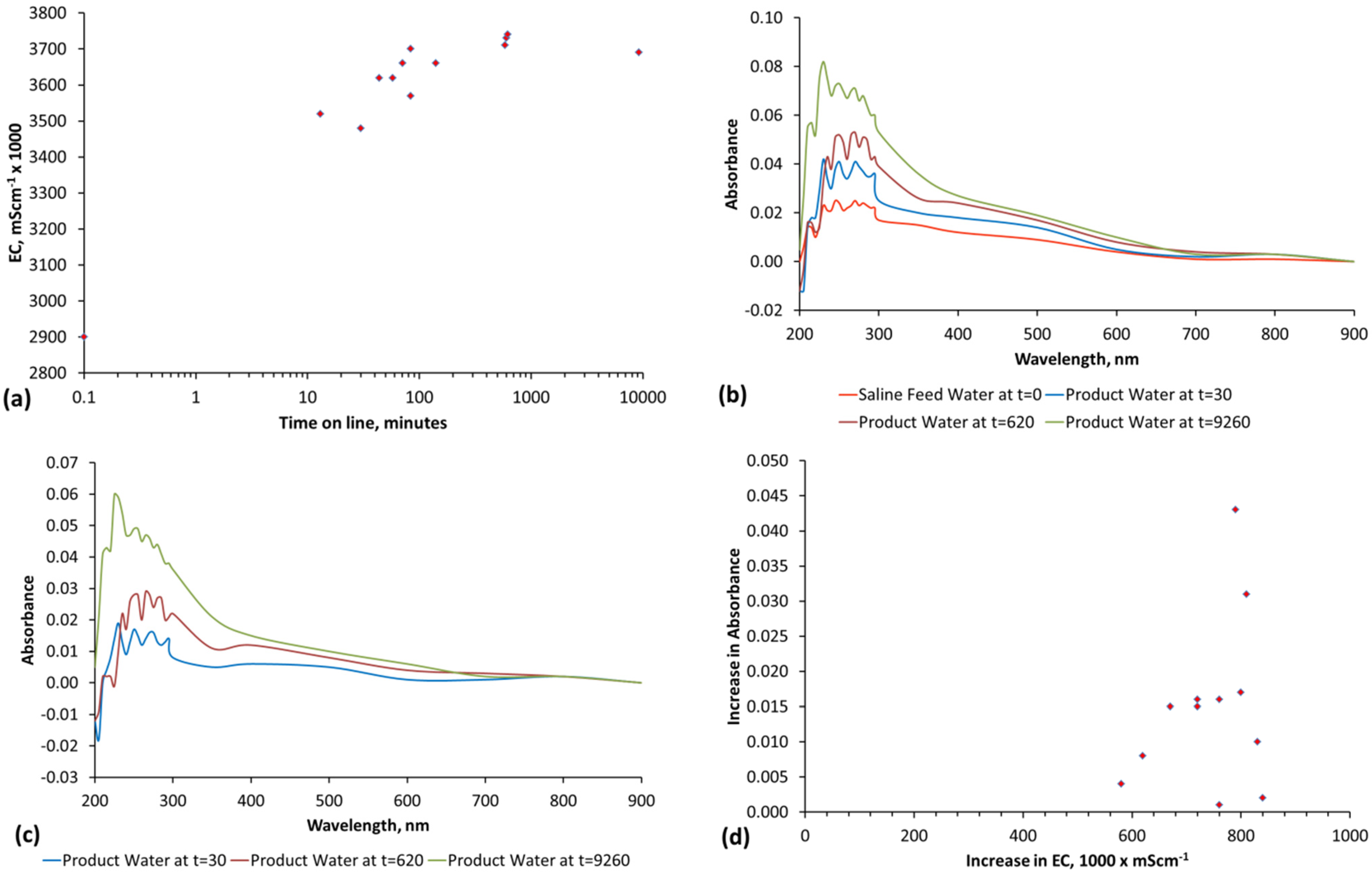

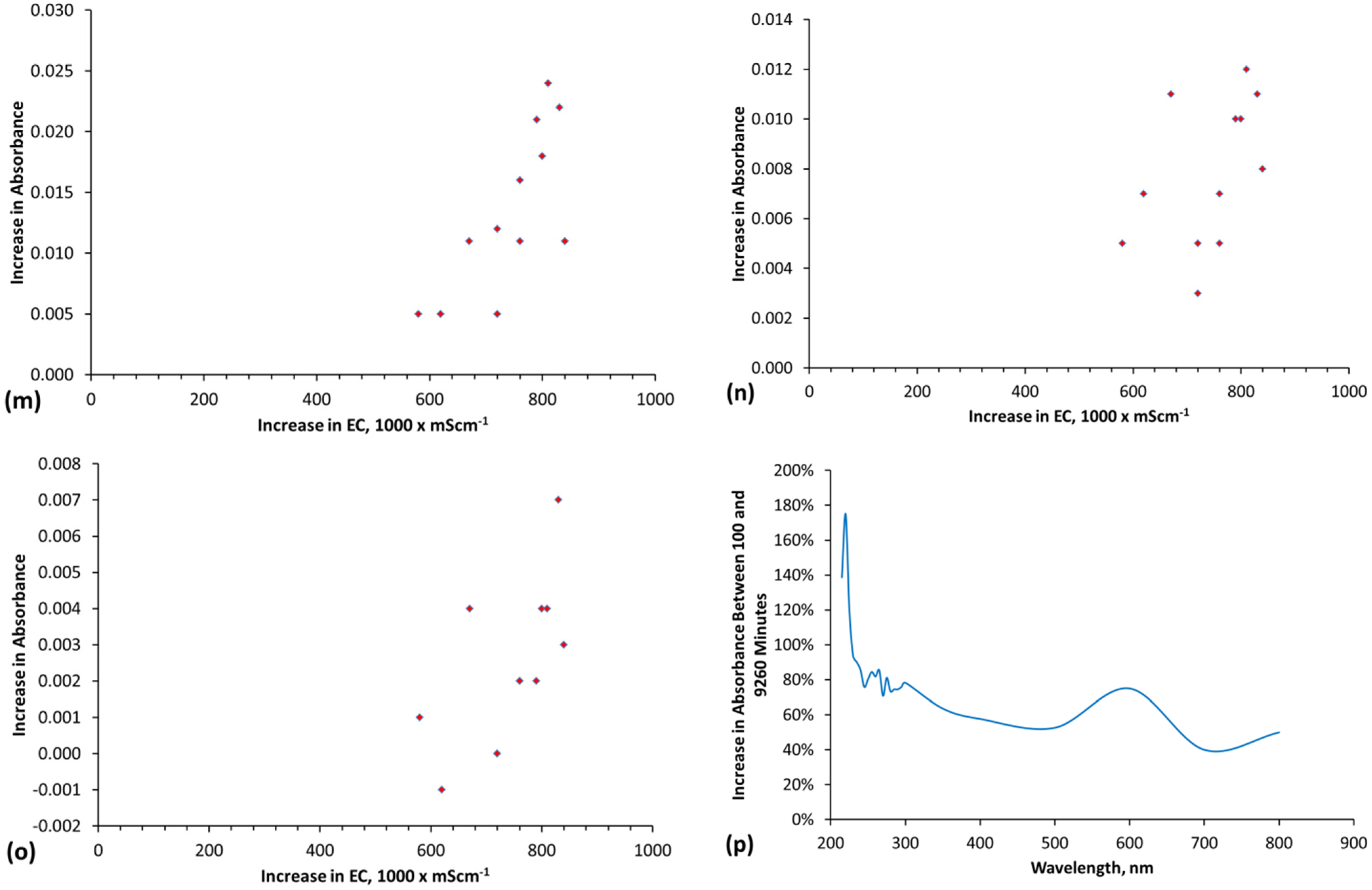
In the example illustrated in Figure E4a,b, [A] = 0.249 mS·cm−1; [B] = 2.651 mS·cm−1. Decreases in NaCl concentration will reduce [B] and will reduce salinity. The observed product water EC after 9260 min = 3.69 mS·cm−1 (Figure E4a). The increase in EC (assuming no desalination) is:
where C = EC attributable to nano-particles added to the feed water by the ZVM TP.
EC = [A] + [B] + [C]
3.69 = 0.249 + 2.651 + [C]
[C] = 3.69 − [0.249 + 3.651] = 0.79
3.69 = 0.249 + 2.651 + [C]
[C] = 3.69 − [0.249 + 3.651] = 0.79
Identification of EC Due to Salinity Decline, when EC Rises Due to Nano-Particle Addition
Stabilisation of the EC after a time, t, (e.g., Figure E4a) can occur as a direct result of either: (i) a cessation of nano-particle addition to the water; or (ii) continued addition of nano-particles to the water which is combined with NaCl removal from the water.
The difference in absorbance between the absorbance at t = n and t = 0 represents the absorbance added by the nano-particles. In the example illustrated in Figure E4a,b, the absorbance added by the nano-particles (Figure E4b,c) continues to increase following stabilisation of the EC (Figure E4a).
A cross-plot of EC increase vs. absorbance increase (at various wavelengths) shows a consistent pattern, where the initial increases in EC are associated with an increase in absorbance (Figure E4d–o). Once a critical maximum increase in EC is achieved, further increases in absorbance occur without increasing EC (Figure E4d–o).
Increases in absorbance with time indicate that the concentration of nano-particles in the water is increasing with time. Therefore the EC attributable to nano-particles [C] will increase with time.
In Figure E4a, the EC becomes constant after 80 min of operation. This indicates that during the initial 80 min of operation [C] > [E]. Thereafter [C] approximates to [E]. Figure E4p demonstrates that the absorbance (and EC) attributable to nano-particles increases, between 100 and 9260 operational minutes, by between 60% and 175%. The nano-particle absorbance pattern (Figure E4p) is consistent (Table 3) with hydrated n-FeOOH (akaganeite) species being present in the water.
The expected increase in [C] (from Figure E4a,p) associated with this increase in nano-particle abundance is 0.48–1.4 mS·cm−1, where 0.48 = 0.6 (from Figure E4p) × [C] (0.79, defined in Equation (56), and 1.4 = 1.75 (from Figure E4p) × [C] (0.79, defined in Equation (56).
It follows that [C] ranges between [0.79 + 0.48] and [0.79 + 1.4]. The expected EC without desalination (i.e., if [D] = 0), and without cation and anion removal (i.e., [E] = 0) is therefore calculated as:
EC9260 min = [A] + [B] + [C] − [D] − [E]
EC9260 min = [0.249] + [2.651] + [1.27 to 2.19] − [0] − [0]
EC9260 min = 4.17 to 5.09 mS·cm−1
EC9260 min = [0.249] + [2.651] + [1.27 to 2.19] − [0] − [0]
EC9260 min = 4.17 to 5.09 mS·cm−1
The observed EC9260 min = 3.69 mS·cm−1 (Figure E4a). The EC has remained constant after 80 to 100 min operation (Figure E4a). If [A] remains unchanged (i.e., [E] = 0), then [D] is between 0.48 and 1.4 mS·cm−1, calculated as EC9260 min (assuming no desalination (4.17 to 5.09 mS·cm−1)) − observed EC9260 min (3.69 mS·cm−1).
The presence of ZVM results in a reduction in feed water cation and anion concentrations. Therefore, [A]9260 min is between 0 and 0.249 mS·cm−1. If [A] is reduced to 0 mS·cm−1 (i.e., [E] = 0.249 mS·cm−1) it follows that:
EC9260 min 3.69 mS·cm−1 = [A] + [B] + [C] − [D] − [E]
EC9260 min = [0.249] + [2.651] + [1.27 to 2.19] − [0.729 to 1.649] − [0.249]
EC9260 min = 3.69 mS·cm−1
EC9260 min = [0.249] + [2.651] + [1.27 to 2.19] − [0.729 to 1.649] − [0.249]
EC9260 min = 3.69 mS·cm−1
The water salinity at 9260 min is assessed as:
Salinty9260 min, mS·cm−1 = [B] − [D]
EC9260 min = [2.651] − [0.729 to 1.649]
Salinty9260 min = 1.002 − 1.922 mS·cm−1
EC9260 min = [2.651] − [0.729 to 1.649]
Salinty9260 min = 1.002 − 1.922 mS·cm−1
The regression relationship between measured EC and measured salinity (Figure E3) indicates that the salinity of the water after 9260 min (6.4 days) is between 0.441 and 0.938 gNaCl·L−1. The salinity removed is between 0.39 and 0.89 g·L−1.
Figure E4 establishes that changes in EC can be directly linked to increases in absorbance which are associated with the formation of nano-particles in the water. Nano-particles, when present as precipitants, will settle when the water is taken out of the reaction environment (Figure E4c–f). Therefore following settlement,
where, C1 = entrained nano-particles and ions which impact on EC; C2 = dissolved ions which do not have a major impact on absorbance; C3 = entrained nano-particles which would be removed by a longer settlement period.
C = C1 + C2 + C3
Appendix F. Summary of the Interaction between Fe Corrosion, Eh, pH, EC and Salinity Removal
Zero Valent Metal (native metal with an oxidation state of zero) is stable and will not oxidize if the water Eh and pH is maintained at specific levels [19]. The trials (Appendix C) demonstrate that the water pH was maintained between pH = 5 and pH = 12 (typically between pH = 7 and pH = 9).
Under these conditions (at 1 atmosphere pressure and at 25 °C),
(1) Aluminium will remain at its water-metal contact as Al0 provided that the Eh is less than [19]:
Eh, V = −1.55 − 0.0591 pH
At higher Eh the dominant product species is Al2O3 (typically Al(OH)3), and the dominant oxidation state is AlIII. At a pH above 8.5 [19] some of the Al2O3 will be present at AlO2− [19]. The relationships between Eh and pH for the different equilibrium aluminium species are provided by: [19,229,230,231]. The Eh and pH of the product water (Figure C1, Figure C2, Figure C3, Figure C4, Figure C5, Figure C6, Figure C7, Figure C8, Figure C9, Figure C10, Figure C11, Figure C12, Figure C13, Figure C14, Figure C15, Figure C16 and Figure C17) indicate that the Al0 is held outside the passivation range, and that the dominant corrosion ion will be AlO2− [19,230]. The transition from Al0 to AlO2− results in both water consumption and the production of H+ (e.g., Al + 2H2O = AlO2− + 4H+(ads) + 3e−; [19,229,230,231]
(2) Copper will remain at its water-metal contact as Cu0 provided that the Eh is less than [19]:
Eh, V = 0.41 − 0.0591 pH
Between this Eh (Equation (62) and the Eh defined in Equation (63), Cu is present as Cu2O (i.e., CuI). At higher Eh it is present as CuO (i.e., CuII). Equation (63) provides the precipitant boundary between CuI and CuII corrosion species [19]:
Eh, V = 0.669 − 0.0591 pH
The Eh and pH of the product water (Figure C1, Figure C2, Figure C3, Figure C4, Figure C5, Figure C6, Figure C7, Figure C8, Figure C9, Figure C10, Figure C11, Figure C12, Figure C13, Figure C14, Figure C15, Figure C16 and Figure C17) indicate that the Cu0 is held outside the passivation range for much of the reaction time, with the dominant precipitated products (in saline water) likely to be CuO and Cu2O [19,232,233,234].
(3) Iron will remain at its water-metal contact as Fe0 provided that the Eh is less than [19]:
Eh, V = −0.44 log(Fe2+ (aq)) for pH = 6 for log(Fe2+ ) = 0 and pH = 9 for log(Fe2+ ) = −6
At higher pH (pH ≥ 9) the boundary is defined as [19]:
Eh, V = −0.047 − 0.0591 pH
The Eh and pH of the product water (Figure C1, Figure C2, Figure C3, Figure C4, Figure C5, Figure C6, Figure C7, Figure C8, Figure C9, Figure C10, Figure C11, Figure C12, Figure C13, Figure C14, Figure C15, Figure C16 and Figure C17) indicate that the Fe0 is held outside the passivation range for much of the reaction time, with the dominant precipitated products (in saline water) likely to be Fe2O3 species, i.e., FeOOH [19,235].
F1. Oxidation of Fe0
Fe0 has an oxidation number of zero. The oxidation number of iron increases as it corrodes [18,19,67,68,69,70,71,72,73,74,75,76,77,78,82,83,84,85,86,87,88,89,90,91,92,93,94,95,96,97,98,99,100,101,102,103,104,111,112,113,114,162,163,164,165,166,167,168,172,173,174,175,176,190,203,204,208,235,236,237,238,239,240]. The initial corrosion product is FeII (e.g., white rust, Fe(OH)2). The FeII gradually replaces the Fe0. With increased oxidation, the white rusts are replaced by, or template the formation of green rusts (platy combinations of FeII and FeIII) (Figure F1). These are then replaced with increased oxidation by yellow to brown to red, to purple, to black rusts (FeOOH). Figure F1 illustrates the morphology of these different rust types and the key features which are involved in the removal of NaCl. Figure F1 demonstrates a number of important points [18,19,72,73,74,75,76,77,78,82,83,84,85,86,87,88,89,90,91,92,93,94,95,96,97,98,99,100,102,103,104,137,138,139,140,162,163,164,165,166,167,168,172,173,174,175,176,190,203,204,208,235,236,237,238,239,240]:
- During corrosion the Fe0 core is initially oxidized to Fe(OH)2.
- The Fe(OH)2 acts as a template for FeOOH growth (rusty purple) around the particle (Figure F1). i.e., a Fe0 particle will corrode to have an Fe0 core, an Fe(OH)2 inner layer (or Fe3O4 inner layer) and an FeOOH outer layer.
- The FeOOH templates the formation of green rust (NaI(a=1−c−b)FeII(b=1−c−a)FeIIIc(OH)2]x−·[(x/n)Cln−·mH2O]x+) sheets growing into the water body from the corroded Fe particle. With increased oxidation these plates gradually transform to FeOOH. In the presence of Cl− ions, any α-FeOOH (goethite) or γ-FeOOH (lepidocrocite) which may initially form, transforms to β-FeOOH (akaganeite) over time. In the presence of HCO3−, CO32− ions, Cl− is replaced in the green rust by CO32−. In the presence of SO42− ions, Cl− (and CO32− ions) are replaced by SO42−. In the presence of SO42− ions, goethite is the dominant FeOOH species and any akagneite formed will transform to goethite. In the presence of high concentrations of HCO3−, CO32− ions the green rust (and some of the FeOOH) may be replaced by FeCO3 [236]. In freshwater, lepidiocrocite and goethite are the dominant FeOOH species. A more detailed analysis of the interaction of HCO3−, CO32−, Cl−, and SO42− ions is provided in Section 6.
- The dissolved Fen+ ions in the water are oxidized to form spherulites of FeOOH which are entrained in the water.
Figure F1.
Corrosion features associated with fibrous (0.1 mm diameter) Fe0 in saline water [PS14], photographed following conclusion of the desalination trial. Black = water filled porosity. Orange/yellow spheroids = hydrated β-FeOOH·mH2O (Fe3+O(O, Cl)) formed by precipitation of Fe3+ ions in the water. Dark grey nodules surrounded by orange spheroids = bog iron (Fe3O4, magnetite). Off white to green and purple sheets growing into the water from the bright white rods = mixed valance green rust complex (NaI(a=1−c−b)FeII(b=1−c−a)FeIIIc(OH)2]x−·[(x/n)Cln−·mH2O]x+, where a + b + c = 1) formed from the accretion of Fe2+ and Fe3+ ions in the water. The bright white rods of Fe(OH)2 pseudomorph after and surround a Fe0 core. They are the initial corrosion product. They are initially replaced at the water interface by purple, β-FeOOH. These act as a template for green rusts (NaI(a=1−c−b)FeII(b=1−c−a)FeIIIc(OH)2]x−·[(x/n)Cln−·mH2O]x+, where a + b + c = 1) sheets. The green rusts are gradually replaced by (β-Fe3+O(O, Cl)·nH2O). The increase in the proportion of FeIII species is initially signified by a rusty purple color which is then replaced by a yellow color when the precipitate is dominated by highly hydrated FeOOH·mH2O. The purple FeOOH becomes increasingly yellow in color with increased hydration. Fe corrosion species in this photograph have been identified by their color and morphology. The left edge (centre) of the photograph truncates a trapped hydrogen gas bubble. The formation of the grey precipitate is associated with the upper surface of the gas bubble. Field of view = 2 cm. The common colors of the various Fe2O3, Fe3O4 corrosion species are: (i) hematite = red; (ii) maghemite = reddish brown; (iii) magnetite = black; (iv) goethite = yellow brown; (v) = lepidococite = orange; (vi) ferrihydrite = red-brown; (vii) akaganeite = purple to red brown/purple to orange/yellow; (viii) layered double hydroxides (white and green rusts) = white to green. The purple colour indicates the incorporation of Na+ (see Appendix H).

NaCl is removed from the overlying water body by:
- Entrapment in the growing FeOOH and (NaI(a=1−c−b)FeII(b=1−c−a)FeIIIc(OH)2]x− [(x/n)Cln−·mH2O]x+) sheets;
- Concentration in the pore water and hydration shells surrounding the FeOOH and (NaI(a=1−c−b)FeII(b=1−c−a)FeIIIc(OH)2]x−·[(x/n)Cln−·mH2O]x+) sheets.
The relationship between Fe corrosion and the presence of NaCl in the water is described further in Appendix G and Appendix H.
F2. Relationship between Eh, pH, Ion Concentration, and Equilibrium Constant, K
For any reaction at STP and at pH = 0, its standard electropotential is defined as ΔE0. This ΔE0 is related to the Standard Gibbs Free Energy ΔG0 for the reaction through the equation [18,19,150]:
where n = number of electrons transferred and F = Faraday constant. These two parameters, ΔE0 and ΔG0 are related to the equilibrium constant, K, standard heat of formation, ΔH0, temperature (K), T, and the standard entropy ΔS0 through the equations [18,19,150]:
ΔG0 = −nF ΔE0
ΔG0 = ΔH0 − TΔS0
ΔG0 = −RT × ln K
ΔE0= RT/nF × ln K
ΔG0 = −RT × ln K
ΔE0= RT/nF × ln K
where R = gas constant It follows from Equation (67), that if the temperature changes, then K, ΔE, ΔG, ΔH, ΔS are also known for the new temperature at a constant pH.
ΔE0 which is defined at pH = 0, can be redefined for the pH observed in the water at time t, where for a reaction converting one ion to another the observed Eh indicates [19]:
Eh = ΔE0 − 0.0591m/n × pH + 0.0591/n × log(MP/MR)
m = number of hydrogen ions transferred; MP = Molar concentration of product ion; MR = molar product of the reactant ion.
The limits of domain between two solid corrosion products, or ZVM and a solid corrosion product become [19]:
Eh = ΔE0 − 0.0591m/n × pH
The limits of domain between an ion and a solid corrosion product becomes [19]:
d = a constant [19].
Eh = ΔE0 − 0.0591m/n × pH + 0.0591/n × log(MP) or for pH independent reactions
Eh = ΔE0 + 0.0591/n × log(MP) or for Eh independent reactions
log(MP) = −d − pH
Eh = ΔE0 + 0.0591/n × log(MP) or for Eh independent reactions
log(MP) = −d − pH
It follows from these relationships that if the temperature, Eh and pH are known for a reaction where ΔE0, or ΔG0 is known, that K, ΔE, ΔG, ΔH, ΔS are also known.
F2.1. Measurement of Eh
Most standard redox meters determine ORP (oxidation reduction potential). They use either platinum, or gold electrodes, and can be supplied in a Ag/AgCl (KCl) gel. Eh is the value referenced to the standard hydrogen electrode (SHE). The relevant measurement standards are defined in British Standard (BS ISO 11271:2002 BS 7755-3.14:2002 [241]) and the international standard ISO 11271:2002 [242]. Depending on the instrument manufacturer, the Eh is either measured directly by the instrument (following use of a suitable calibration fluid, e.g., calomel, KCl, quinhydrone), or the Eh is calculated as [243,244,245,246,247,248]:
Eh, mV = ORP + Em
ORP = Oxidation – reduction potential, mV, measured by a standard pH/ORP meter, ORP meter, or ORP electrode. Em varies with temperature and is calculated as:
Em = ESHE − ERef
ESHE = The Eh of the standard hydrogen electrode (e.g., ESHE = −2.3591T + 483.82); T = temperature, °C; ERef = The ORP reading in the calibration fluid (e.g., 3 M KCl saturated with Ag/AgCl, ERef = −1.6284T + 259.18). A variety of different calibration fluids and correlations are available.
F2.2. Removal of NaCl in a Redox Environment
NaCl remains as Na+ and Cl− ions in an aqueous environment [19]. These ions can be incorporated in two Fe corrosion species, ferrous hydroxychloride (Green Rust) [69,75] and akaganeite [70,87,88,96] (Figure F1).
Alternatively they can be held in the hydration shells surrounding FeOOH spp. and the green rust. In this instance, the relationship between Eh and pH may control the relative amount of NaCl held in the hydration shells:
where MHS = NaCl held in hydration shells; MRS = residual NaCl held in the water. The total amount of NaCl, MtS, in the reaction environment is:
Eh = ΔE0 − 0.0591m/n × pH + 0.0591/n × log(MHS/MRS)
MtS = MHS + MRS
Once the hydration shells become saturated, log(MHS/MRS) will remain constant. log(MHS/MRS) is a measure of the residual salinity [F] in the water where [F] = ([A] − [D]), and [F], [A] and [D] can be measured. MHS is a function of [D] and MRS is a function of [F]. It follows that the salinity which results in the hydration shells become saturated [F] will result in a constant EC being observed.
This situation is defined in this study as an equilibrium position, but could be defined as pseudo-equilibrium position or a steady state position. In Figure C5, Figure C6, Figure C7, Figure C8 and Figure C9, the abrupt switch from a declining EC with time, to a constant EC (or slightly declining EC) with time, is accompanied by relatively constant values of pH and Eh. This suggests, from Equation (73) that the constant EC represents a period where log(MHS/MRS) is constant (i.e., is in a stable equilibrium).
If EC, Eh and pH are constant, then it follows that the chemical relationship between the NaCl dissolved in the water and the NaCl which has been removed by the ZVM TP is in equilibrium. All references to equilibrium involving a steady state EC, pH and Eh in this study reflect this definition.
It follows from Equations (66)–(68) that if the equilibrium value of Eh is known, that the equilibrium values of K, ΔE, ΔG, ΔH, ΔS are also known.
Figure F2 illustrates a typical example where EC stabilizes to an equilibrium position. This equilibrium position is associated with a stable Eh and pH (Figure C5). The example demonstrates 134 oscillations in EC, which can be interpreted [18] as galvanic charge:discharge cycles. The exponential decline in EC, under this model, reflects a specific capacity (specific capacitance) which reduces with time. The Columbic efficiency, at the point equilibrium is reached is 0%.
The Columbic efficiency, Ce [122] is calculated as,
td = discharge time: tc = charging time.
Ce = td/tc × 100
FeOOH nano-rods grown on a carbon substrate have been demonstrated to operate as capacitors over 5000 charge:discharge cycles without a decrease in capacitance [129]. The specific capacitance of the FeOOH decreases as the structure becomes laminated [129], e.g., through the accretion of green rust layers (Figure F1), or accretion and coalescence of FeOOH colloids (Figure F1). Increasing the C:FeIII proportion can increase the specific capacitance [130], e.g., through the presence of CO32− ions, as demonstrated by PS15 and PS16. The structuring of the FeOOH nanorods as colloidal, or spherical, or flower like structures can increase their specific capacitance [131], e.g., Figure F1.
Figure F2.
Impact of progressively reducing water salinity on the rate of desalination with time. ZVM TP Trial ST1a: Extracted from Figure C5.
Figure F2.
Impact of progressively reducing water salinity on the rate of desalination with time. ZVM TP Trial ST1a: Extracted from Figure C5.
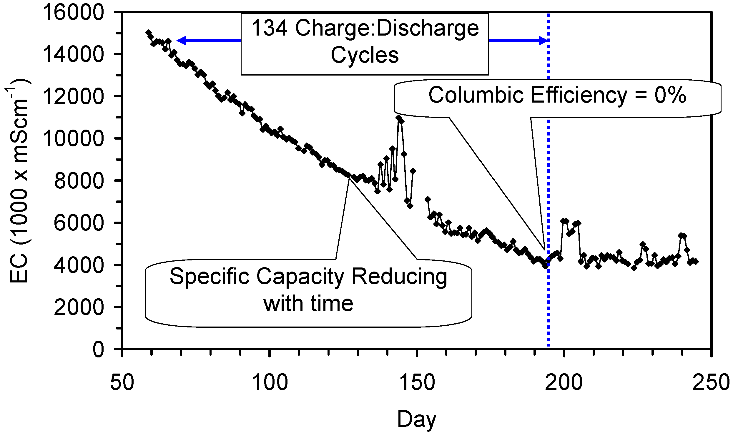
F3. Relationship between EC and Reaction Kinetics
Salinity reduction by reaction, catalysis, or adsorption involves reaction kinetics [18]. This allows quantitative data such as EC (or salinity) to be reconfigured in terms of temperature, T, ZVM TP/TPA concentration, particle size and particle surface area [18].
An understanding of how EC changes are related to reaction kinetics can allow the rate of desalination to be increased, the cost of desalination to be decreased, and both the amount of, and composition of, the ZVM TP to be optimised. It can also provide a commercial and technical basis for understanding both the desalination behaviour and variability associated with a specific batch of ZVM TP.
The interaction of kinetics with desalination can be assessed as follows:
- The magnitude of [D] is a function of the reaction rate, k, where [18]:kobserved = kactual × [Pw] × [as]
Where [Pw] = amount of ZVM, g·L−1; [as] = surface area of ZVM, m2·g−1.
kobserved = observed reaction rate; kactual = actual reaction rate. - For a constant [Pw], [D] will decrease as [as] decreases (i.e., the length of time required to reduce the salinity of water from x g·L−1 to y g·L−1 will increase as [as] decreases).
- kobserved is therefore a function of [Pw] and [as].
- The cost of desalination reduces as: (i) [Pw] decreases; (ii) [as] decreases; and (iii) kactual increases.
This model (Equation (77)) assumes [18] that the ZVM TP acts as a catalyst (or adsorbent), the number of catalytic/adsorbent sites is a function of surface area [as], and the number of catalytic/adsorbent sites remains constant with time.
If the ZVM TP acts as a catalyst (or reactant) where the process involves adsorption and desorption, then a proportion of the available sites at time t = 0 may be unavailable at time t = n. The same situation will also arise if the ZVM TP becomes progressively oxidised with time, or reacts with components in the water with time. In this instance the magnitude of [D] becomes a function of the reaction rate, k, [18] where:
Where [aa] = the proportion of sites present in the ZVM that are available at time t. [aa] will decrease with time as sites become utilised/blocked. [aa] can increase with time, if the growing Fe corrosion products create new sites (e.g., Figure F1).
kobserved = kactual × [Pw] × [as] × [aa]
F3.1. Assessment of the Impact of Changing [as] and [aa] on Salinity
The measured 24 h regression relationship between Cl− concentration in the feed and product waters at t = 0 [21] can be used to demonstrate the impact of changing [as] and [aa] on desalination.
The impact of decreasing [as] is to increase the length of time it takes for the water salinity to reduce from a level [x] to a level [y] where:
where [Wst=0] = water salinity at t = 0; [Wst=1] = water salinity at t = 1. [CWt=1] = water salinity at t = 1 corrected for the change in [Pw], [as] and [aa] relative to the reference standard used to calculate the regression correlation [21]. Reference standards: [Pw] = 20 g·L−1; [as] = 77.26 m2·g−1; [aa] = 1.0 [20,21].
Predicted 24 h salinity change for [as] = 1, (Regression Equation from [21]):
[Wst=1] = 1.1[Wst=0]0.98
Corrected 24 h salinity change for c = ([Pw] × [as] × [aa])actual/([Pw] × [as] × [aa])reference = 0.5
[CWt=1] = [Wst=0] − (c([Wst=0] − (1.1[Wst=0]0.98))
[Wst=1] = 1.1[Wst=0]0.98
Corrected 24 h salinity change for c = ([Pw] × [as] × [aa])actual/([Pw] × [as] × [aa])reference = 0.5
[CWt=1] = [Wst=0] − (c([Wst=0] − (1.1[Wst=0]0.98))
A value of [as]actual/[as]reference = 0.5 indicates that the effective surface area is half the surface area of the reference standard [21] used to construct the regression relationship (e.g., 38.6 m2·g−1).
The impact of reducing [aa] is to reduce the amount of desalination that can occur for a specific value of [as] as [aa] = [aa]actual/[aa]reference:
Predicted 24 h salinity change for [as]actual/[as]reference = 1
[Wt=1] = 1.1[Wt=0]0.98
Corrected 24 h salinity change for [as] = 1.0; [aa] = 0.9
[CWt=t+1] = [Wt=t] − ([at+1]([Wt=t+1] − (1.1[Wt=t]0.98))
[at+1] = ([as]actual/[as]reference) × ([aa]actual/[aa]reference) × ([Pw]actual/[Pw]reference) × ([k]actual/[k]reference)
[Wt=1] = 1.1[Wt=0]0.98
Corrected 24 h salinity change for [as] = 1.0; [aa] = 0.9
[CWt=t+1] = [Wt=t] − ([at+1]([Wt=t+1] − (1.1[Wt=t]0.98))
[at+1] = ([as]actual/[as]reference) × ([aa]actual/[aa]reference) × ([Pw]actual/[Pw]reference) × ([k]actual/[k]reference)
The impact of changing the [as] and [aa] ratios (when [Pw] remains constant) is shown in Figure F3. In Figure F3 the following calculation assumptions are made:
[as] = Reference ZVM Surface Area, m2·g−1 = 77.26 m2·g−1
[Pw] = Reference ZVM concentration, g·L−1 = 8 g·L−1
[aa] = Reference % of ZVM surface area available for adsorption = 100%
[Pw] = Reference ZVM concentration, g·L−1 = 8 g·L−1
[aa] = Reference % of ZVM surface area available for adsorption = 100%
Curve fitting can be used to replicate the EC declines associated with ZVM TP desalination (Figure C1, Figure C2, Figure C3, Figure C4, Figure C5, Figure C6, Figure C7, Figure C8, Figure C9, Figure C10, Figure C11, Figure C12, Figure C13, Figure C14, Figure C15, Figure C16 and Figure C17). This allows the relative success of the various ZVM TP pre-treatments (and ZVM compositional combinations) to be evaluated. These pre-treatments are designed to take ZVM with a low [as] and increase the associated kactual.
Figure F3.
Expected decline in EC with time. (a) Impact of changing [as] when [aa] = 1.0; [Pw] = 1.0; (b) Impact of changing [aa] when [as] = 1.0; [Pw] = 1.0. Equation based on Cl− adsorption rates for Fe0 [21]. [aa] = ([as]actual/[as]reference); [aa] = ([aa]actual/[aa]reference); [Pw] = ([Pw]actual/[Pw]reference).

G. Fe Corrosion Species Involved in Desalination
The precipitated Fe corrosion species which could potentially be present in the ZVM TP/TPA + water during desalination fall into three groups [18,19,67,68,69,70,71,72,73,74,75,76,77,78,82,83,84,85,86,87,88,89,90,91,92,93,94,95,96,97,98,99,100,102,104,111,112,113,114,162,163,164,165,166,167,168,172,173,174,175,176,190,203,204,208,236,237,238,239,240]:
- Reduced Fe corrosion products, e.g., magnetite (Fe3O4) and related species.
- White and green rusts, i.e., Fe(OH)2 and layered hydroxides (green rusts).
- Brown rusts, i.e., Fe(OH)3, FeOOH spp.
The dominant precipitant (either in the water as entrained particles, or accreting onto surfaces), is controlled by the temperature, pressure, Eh, pH, and both the relative and absolute concentrations of Cl−, HCO3−, CO32−, S2−, HS−, SO42−, OH−, Fen+, and H+ ions in the water [19].
Detailed historical experiments documented in this study have clearly identified a number of reaction pathways which consistently occur. These pathways are:
- (1)
- In freshwater containing no Cl−, HCO3−, CO32−, S2−, HS−, SO42− ions the reaction sequence is as follows:
- (a)
- Stage 1: Fe0 corrodes to Fe(OH)2
- (b)
- Stage 2: Fe(OH)2 corrodes to Fe(OH)3 and FeOOH (lepiocrocite and goethite). H+(ads) ions may reduce Fe(OH)2 which is adjacent to the Fe0 to Fe3O4 (magnetite).
- (2)
- In freshwater containing no Cl−, S2−, HS−, SO42− and containing HCO3−, CO32− ions the reaction sequence is as follows:
- (a)
- Stage 1: Fe0 corrodes to Fe(OH)2
- (b)
- Stage 2: Fe(OH)2 corrodes to GR1(CO32−) which corrodes to Fe(OH)3 and FeOOH (lepiocrocite and goethite). H+(ads) ions may reduce Fe(OH)2 which is adjacent to the Fe0 to Fe3O4 (magnetite). In the presence of SO42− ions GR1 is replaced by GR2(SO42−) and the CO32− ions are expelled into the water.
- (3)
- In saline water containing no HCO3−, CO32−, S2−, HS−, SO42− ions the reaction sequence is as follows:
- (a)
- Stage 1: Fe0 corrodes to Fe(OH)2
- (b)
- Stage 2: Fe(OH)2 corrodes to GR1(Cl−). The GR1(Cl−) corrodes to form FeOOH. The dominant FeOOH sp. is akaganeite. Any lepiocrocite and goethite which form as an intermediate stage are transformed over the longer term to akaganeite. H+ (ads) ions may reduce Fe(OH)2 which is adjacent to the Fe0 to Fe3O4 (magnetite).
- (4)
- In saline water containing HCO3−, CO32− ions and no S2−, HS−, SO42− ions the reaction sequence is as follows:
- Stage 1: Fe0 corrodes to Fe(OH)2
- Stage 2: Fe(OH)2 corrodes to GR1(CO32−). The GR1(CO32−) corrodes to form FeOOH. The dominant FeOOH sp is akaganeite. Any lepiocrocite and goethite which form as an intermediate stage are transformed over the longer term to akaganeite. H+(ads) ions may reduce Fe(OH)2 which is adjacent to the Fe0 to Fe3O4 (magnetite). In the presence of SO42− ions GR1 is replaced by GR2(SO42−) and the Cl− or CO32− ions are expelled into the water and the final FeOOH product is goethite. In the presence of S2−, HS− ions, Fe(OH)2 and FeOOH corrode to FexSy and S precipitates.
The trials documented in Figure C1, Figure C2, Figure C3, Figure C4, Figure C5, Figure C6, Figure C7, Figure C8, Figure C9, Figure C10, Figure C11, Figure C12, Figure C13, Figure C14, Figure C15, Figure C16, Figure C17, Figure C18, Figure C19, Figure C20, Figure C21, Figure C22, Figure C23, Figure C24, Figure C25, Figure C26, Figure C27, Figure C28, Figure C29, Figure C30, Figure C31, Figure C32, Figure C33, Figure C34, Figure C35, Figure C36 and Figure C37 were operated in saline water containing 1000–22,000 mgCl−·L−1, 10–150 mg·L−1 [HCO3−, CO32−], no [S2−, HS−] and 1–5 mg·L−1·SO42− ions the reaction sequence. Consequently the species expected are Fe(OH)2, GR1(Cl−), FeOOH (akaganeite) and Fe3O4 (magnetite). The Eh, pH regimes indicate that the dominant corrosion product entrained in the water is FeOOH.
Any chemical analysis of ZVM TP during desalination (e.g., Figure F1) is likely to demonstrate the presence of white rust, green rust, magnetite, and akagangeite, but may also demonstrate the presence of goethite and lepidocrocite [68,204]. These create anodic and cathodic sites within the ZVM TP/TPA and surrounding water [18,203], and as demonstrated in this study, this allows currents, voltages, resistance, and capacitance to be measured.
The overall process of Na+ and Cl− capture by the charged Fe corrosion products remains unknown, but is investigated further in Appendix H.
Appendix H. Identification of the Radicals Involved in NaCl Removal
The anion and cation analyses (Table C1, Table C2, Table C3 and Table C4) demonstrate that there is no net increase in soluble Fe ions in the product water relative to the feed waters when the desalination involves ZVM TP. Small concentrations of entrained nano-Fe corrosion products (and n-Fe) can create substantial increases in water EC. In these situations measurement of an absorbance spectrum of fresh product water [G], and measurement of an absorbance spectrum of the product water after the water has been allowed to rest and some of the entrained particles have been allowed to settle [H] will allow the UV-visible absorbance spectrum [J] of the entrained (settled) particles to be determined (Table 3). For each wavelength analysed:
[J] = [G] − [H]
The UV-Visible spectra of the low concentrations of entrained nano-particles in the water associated with the E146 trial were determined (Figure C37). These spectra indicate that the dominant nano-particle is hydrated akaganeite (Table 3).
Each spectra displays a number of peaks and troughs over the spectral range 200–300 nm. These peaks can be interpreted in terms of the OH radicals, Fe ions, Cl ions, and Na ions.
The absorbance associated with the OH radical ([OxH–H2O]•n+/−) can result from a dissolved gas phase transition (associated with the air, or N2:CO2 gas feed). This type of transition is termed AX [32].
Absorbance associated with the OH radical ([OxH–H2O]•n+/−) involving the transfer of an electron from a closed shell solvent (e.g., H2O) into the valance hole of a radical solute is termed CT [32].
The absorption peaks associated with specific molecular species and ions at different wavelengths include:
- (1)
- Fe0 [227]: 216 nm, 268 nm (minor);
- (2)
- (3)
- Fe-Ion exchange material [226]: 500–550 nm;
- (4)
- (5)
- ClO2 [217]: 292 nm;
- (6)
- ClO− [228]: 290 nm;
- (7)
- NaClO [228]: 291.4 nm;
- (8)
- HClO [217]: 360 nm;
- (9)
- ClOOCl [219]: 250 nm;
- (10)
- OH–H2O• Radical Structures [221,222,223,224];
- (a)
- AX transition (adsorption of OH radical from the gas phase):
- (i)
- Free OH: 263 nm; 277–288 nm; 299–306 nm;
- (ii)
- OH–H2O• Structures—AX transition: H-bond donor structure C1: 244 nm; 289 nm; 310–334 nm;
- (iii)
- OH–H2O• Structures—AX transition: H-bond acceptor structure C3: 263 nm; 278–290 nm; 299–300 nm; 327 nm;
- (iv)
- OH–H2O• Structures—AX transition: hemi-bonded structure C2: 220 nm; 252 nm; 266–282 nm;
- (b)
- CT transition (adsorption of OH radical from the water):
- (i)
- H-bond acceptor structure C3: 223–229 nm; 245–249 nm; 258–265 nm; 676 nm;
- (ii)
- OH–H2O Structures—CT transition: hemi-bonded structure C2: 211–217 nm; 228–231 nm;
- (11)
- HO2− [225]: 225 nm;
- (12)
- O2− [225]: 245 nm;
- (13)
- Cl− [238]: 210–220 nm;
- (14)
- NaO− [249]: 262/8 nm, 275/6 nm, 301 nm, 324/8 nm, 337 nm, 351 nm, 365 nm, 395 nm.
Analysis of the absorbance in the 200–300 nm wavelength (Figure C37) indicates the presence of a variety of OH–H2O radicals, which are either derived from the solute (water, CX series) or gas interactions (AX series). The dominant radical structure is a CT-hemi-bonded, or CT H-bond acceptor structure (e.g., HO2−).
The dominant AX-series radicals (Figure C37) are H-bond acceptor radicals and hemibonded radicals. The dominant CT-series radicals (Figure C37) are also H-bond acceptor radicals and hemibonded radicals. H-bond acceptor radicals can take the form [(H2O)n(H3O+)m(OxH)y]• (and include radicals containing the HO2− ion), or hemibonded radicals or dimers. The (OxH)y ion complex can be charged. Proton based structures are preferred by (H2O)n•(+) radicals, while hemibonded structures are preferred by (HCl)n•(+) radicals.
A higher proportion of HO2− bonded radicals can be present when the feed gas includes CO2 (Figure C37af,ar).
The observation (e.g., Figure C37aj) that Cl can be bound to Fe (as FeCl2+) is consistent with existing akaganeite and GR1 models. Cl (Figure C37j,ag) can be present as ClOOCl, ClO2 and HClO within the hydrated nano-particle structure. Some of the ClO2 identified in Figure C37 will be ClO− (e.g., Figure C37j). ClO− and ClO2 have virtually identical spectral peaks at 290/292 nm. Conventional modeling of the hydrated shell assumes that the Cl is held as Cl−, and does not assume that the water is highly oxygenated, or that the Cl is held in H2O radicals [96].
The ClO− can be formed via the reaction of an OH-H2O couplet with Cl−, e.g.,
Cl− + OH− = HClO + 2e−
ClO− + 0.5H2 = HClO + e−
E1: Cl− + OH− = ClO− + H+ + 2e−
ΔH0 = 122.9 kJ·M−1; ΔG0 = 122.9 kJ·M−1; ΔE0 = −0.623 V
E2: Cl− + OH− = ClO− + 0.5H2 + e−
ΔH0 = 122.9 kJ·M−1; ΔG0 = 122.9 kJ·M−1; ΔE0 = −1.24 V
Eh = ΔE0 − 0.0591m/n × pH + 0.0591/n × log[Cl−/ClO−]
Eh (E1), V = −0.623 − 0.02955 × pH + 0.02955 × log[Cl−/ClO−]
Eh (E2), V = −1.24 − 0.0591 × pH + 0.0591 × log[Cl−/ClO−]
E3: 2Cl− + O2− = 2ClO− + 2e−
ΔH0 = −107.1 kJ·M−1; ΔG0 = −36.8 kJ·M−1; ΔE0 = 0.381 V
Eh (E3), V, = 0.381 − 0.02955 × pH + 0.02955 × log[Cl−/ClO−]
m = number of H+ ions; n = number of electrons transferred
The Eh–pH relationships required by Equation (82) to produce ClO− were not observed in trials E145, E146. O2− ions were observed in the nano-particles, e.g., Figure C37p. This provides an alternative reaction route, e.g.,
E3: 2Cl− + O2− = 2ClO− + 2e−
ΔH0 = −107.1 kJ·M−1; ΔG0 = −36.8 kJ·M−1; ΔE0 = 0.381 V
Eh (E3), V, = 0.381 − 0.02955 × pH + 0.02955 × log[Cl−/ClO−]
ΔH0 = −107.1 kJ·M−1; ΔG0 = −36.8 kJ·M−1; ΔE0 = 0.381 V
Eh (E3), V, = 0.381 − 0.02955 × pH + 0.02955 × log[Cl−/ClO−]
The Eh-pH relationships required by Equation (83) to produce ClO− were observed in trials E145, E146 (Figure C19, Figure C20, Figure C21, Figure C22, Figure C23, Figure C24, Figure C25, Figure C26, Figure C27, Figure C28, Figure C29, Figure C30, Figure C31, Figure C32, Figure C33, Figure C34, Figure C35 and Figure C36). This indicates that the first stage in the desalination process involves O2, e.g., Figure C37ah,aj:
O2 + FeOH+ = FeOH2+ + O2−
ΔH0 = 33.9 kJ·M−1; ΔG0 = 48.0 kJ·M−1; ΔE0 = −0.497 V
Eh (E4), V = −0.497 − 0.0591 × pH + 0.0591 × log[FeOH+/FeOH2+]
ΔH0 = 33.9 kJ·M−1; ΔG0 = 48.0 kJ·M−1; ΔE0 = −0.497 V
Eh (E4), V = −0.497 − 0.0591 × pH + 0.0591 × log[FeOH+/FeOH2+]
An alternative route is:
O2 + Fe2+ = Fe3+ + O2−
ΔH0 = 40.6 kJ·M−1; ΔG0 = 74.2 kJ·M−1; ΔE0 = −0.768 V
Eh (E5), V = −0.768 − 0.0591 × pH + 0.0591 × log[Fe2+/Fe3+]
Fe2+ = Fe3+ + e−
O2 + e− = O2−
ΔH0 = 0 kJ·M−1; ΔG0 = 0 kJ·M−1
ΔH0 = 40.6 kJ·M−1; ΔG0 = 74.2 kJ·M−1; ΔE0 = −0.768 V
Eh (E5), V = −0.768 − 0.0591 × pH + 0.0591 × log[Fe2+/Fe3+]
Fe2+ = Fe3+ + e−
O2 + e− = O2−
ΔH0 = 0 kJ·M−1; ΔG0 = 0 kJ·M−1
In addition to the reaction route forming akaganeite/GR1 via a FeClmn+ structure (e.g., Figure C37n,ar,ah), the analyses (Figure C37) indicate that a reaction route via ClO− (or ClO2) is responsible for the removal of some Cl−. Some ClO–OCl dimer structures were observed, e.g., Figure C37j,l. They may be formed as:
ClO− = ClO + e−
ΔH0 = −4.6 kJ·M−1; ΔG0 = 83.7 kJ·M−1
2ClO = ClO–OCl
ΔH0 = 0 kJ·M−1; ΔG0 = 0 kJ·M−1
ΔH0 = −4.6 kJ·M−1; ΔG0 = 83.7 kJ·M−1
2ClO = ClO–OCl
ΔH0 = 0 kJ·M−1; ΔG0 = 0 kJ·M−1
Studies of FeIII crystallization in the presence of ClOxn− ions have demonstrated that they assist in the formation of polymerized (polymeric) FeOOH structures [250]. Previous studies have focused on the use of ClO4n− ions [239,250]. They have established that goethite is the predominant polymeric FeOOH structure in the presence of ClO4n− ions, while akaganeite is the dominant FeOOH structure in the presence of Cl− ions [239]. The ClO−, ClO–OCl and HClO structures incorporated within hydrated akaganeite nano-particles (including the ionic and hydrated shells) can be attributed to the oxygenated reaction conditions used in Trials E145, E146 (Figure C19, Figure C20, Figure C21, Figure C22, Figure C23, Figure C24, Figure C25, Figure C26, Figure C27, Figure C28, Figure C29, Figure C30, Figure C31, Figure C32, Figure C33, Figure C34, Figure C35 and Figure C36).
The entrapment of NaCl in the growing polymeric FeOOH/GR1 structures may take the form:
NaCl = Na+ + Cl−
Reaction Demonstrated by Figure C37 at wavelength 245 nm
O2 + e− = O2−
Reaction demonstrated by pH changes with time (Figures C19–C36)
0.5O2− + H2O = HO-OH + 2e− = 2OH−
Reaction Demonstrated by Figure C37 at wavelength 225 nm
HO–OH + OH− = HO2− + H2O
Reactions Demonstrated by Figure C37 at wavelength 290 nm
2Cl− + O2− = 2ClO− + 2e−
Reactions Demonstrated by Figure C37 at wavelength 250 nm
ClO− = ClO + e−
Cl− + H2O + O2 = OH− + HO-OCl
ClO− + H2O2 = ClO + OH + OH−
ClO− + HO2− = ClO + 0.5O2− + OH−
2ClO = ClO–OCl
ClO + OH = HO–OCl
Reaction [238] demonstrated by Figure C37 at 240 nm
O2− + Fe2+ = Fe3+ + O22−
Reactions demonstrated by Figure C37 at 265 nm and 275 nm
2Na+ + O22− = 2NaO−
It has been suggested [190] that during desalination the Fe corrosion products behave as electrochemical, switchable, redox moieties, where the initial Fe0 is modified during corrosion to contain tethered cathodic (e.g., H+, FeHn+, FeO(OH)nx+) groups and tethered anodic (e.g., On−, OH−, O2H−, FeO(OH)nx−) groups, where the tethered cathodic groups form ion adducts with anions and the tethered anodic groups form ion adducts with cations. This study has established (Figure C37) that the ions attached to the tethering sites (which can include akaganeite, goethite, lepidocrocite and ferrate) include: (i) anions: NaO−, ClO−, OH−, Onm−, HO2−; (ii) neutral species: ClO–OCl, HO–OCl, HClO, ClO2; (iii) cations: Fe3+, FeOH2+, FeCl2+.
The presence of purple FeOOH species (Figure F1) is indicative of Na inclusion. Na inclusion can take the form (e.g., Figure C37), 2FeOOH + 2 NaO− = Fe(OH)2 + Na2FeO4 + 2e− [251]. Ferrate(IV) salts form at temperatures of <30 °C [251,252] from the anodic corrosion reaction series reaction (Fe0 + 8OH− = FeO42− + 2H2O + 6e−) and the cathodic reaction (2H2O = 2H+ + 2OH−) and FeO42− + 2Na+ = Na2FeO4 [250]. Their yield is maximized by a current density of 3 mA·cm−2, and the current efficiency increases as the carbon content of the Fe increases, e.g., a current efficiency of >70% applies when the Fe contains >0.9% C [252]. The formation of the ferrate salt is facilitated by the presence of ClO− (Figure C37) (Fe2+ + 4OH− + 2ClO− = FeO42− + 2Cl− + 2H2O [253]). The ferrate formation is facilitated by the analyte (pore water) containing >0.02 wt % Cl−, and is optimized by a weight ratio in the pore waters of NaOH:NaCl (or OH:Cl) of between 25:1 and 5000:1 [254]. This indicates that Cl removal in GR1 and FeOOH from the analyte facilitates the subsequent removal of Na+ by the FeOOH structures (Figure F1). The Cl− ion catalyses the formation of ferrate at the FeOOH—water interface, and within the corroded Fe products, where it facilitates transport of the ferrate in bulk solution to the FeOOH-water interface [254]. The efficiciency of the ferrate formation process increases with temperature in the range 0–60 °C [254]. At 44 °C, with a current of 0.17 A, and voltage of 2.79 V (current density = 48 mA·cm−2), the current efficiency (of ferrate production) is >92% [254]. Figure 11 indicates that the natural current density of the ZVM TP (Cell 2) was 0.6 mA·cm−2. The current efficiency of ferrate production and Na removal decreases with decreasing temperature [254]. This decrease can only be offset partially by increasing the current density.
The ZVM TP data (Figure 11, Figure 12 and Figure 13) establishes (Figure H1) that fresh ZVM TP/ZVM (L1, L2, L5) and ZVM TP following desalination (L4) occupy different fields. The fresh ZVM TP/ZVM has a lower current density: voltage ratio than the ZVM TP following desalination (Figure H1). These observations allow measurements of current and voltage to be used to assess the likely potential effectiveness of a ZVM TP batch for desalination. This analysis indicates that desalination will effectively cease, when the ZVM TP looses the ability to incorporate addition Na ions into a corrosion product.
Figure H1.
Relationship between current density and voltage associated with ZVM TP. L1 to L4 are defined in Figure 13. L5 is the measured relationship between voltage and current density associated with a current efficiency (Fe3+ removal to form ferrate) of 50%–92% over 1 h at 35–50 °C [254]. Relative current density, mA·cm−2 = 48 × ((Voltage (V) × Current (A))/(0.17 × 2.79)) [254].

References
- Zang, Y.; Liu, Y.; Jing, Y.; Zhao, Z.; Quan, X. Steady performance of a zero valent iron packed anaerobic reactor for azo dye waste water treatment under variable influent quality. J. Environ. Sci. 2012, 24, 720–727. [Google Scholar] [CrossRef]
- Li, S.; Wang, W.; Yan, W.; Zhang, W.X. Nanoscale zero valent iron (nZVI) for the treatment of concentrated Cu(II) wastewater: A field demonstration. Environ. Sci. Process Impacts 2014, 16, 524–533. [Google Scholar] [CrossRef] [PubMed]
- Ma, L.; Zhang, W.-X. Enhanced biological treatment of industrial waste water with bi-metallic zero-valent iron. Environ. Sci. Technol. 2008, 42, 5384–5389. [Google Scholar] [CrossRef] [PubMed]
- Rima, J.; Rahme, K.; Assaker, K. Advanced oxidation of olive mill waste water OMW by an oxidative free-radical process induced with zero valent iron. J. Food Res. 2014, 3, 70–82. [Google Scholar] [CrossRef]
- Antia, D.D.J. Sustainable zero-valent metal (ZVM) water treatment associated with diffusion, infiltration, abstraction and recirculation. Sustainability 2010, 2, 2988–3073. [Google Scholar] [CrossRef]
- Antia, D.D.J. Modification of aquifer pore water by static diffusion using nano-zero-valent metals. Water 2011, 3, 79–112. [Google Scholar] [CrossRef]
- Gavaskar, A.; Tatar, L.; Condit, W. Cost and Performance Report: Nanoscale Zero-Valent Iron Technologies for Source Remediation; Contract Report CR-05-007-ENV; Naval Facilities Engineering Command, Engineering Service Center (NAVFAC): Port Hueneme, CA, USA, 2005; p. 44. [Google Scholar]
- Cunningham, J.A.; Reinhard, M. Injection-extraction treatment well pairs: An alternative to permeable reactive barriers. Ground Water 2002, 40, 599–607. [Google Scholar] [CrossRef] [PubMed]
- Mackenzie, K.; Schierz, A.; Georgi, A.; Kopinke, F.-D. Colloidal activated carbon and carbo-iron-novel materials for in-situ groundwater treatment. Glob. NEST J. 2008, 10, 54–61. [Google Scholar]
- Cundy, A.B.; Hopkinson, L.; Whitby, R.L.D. Use of iron-based technologies in contaminated land and groundwater remediation: A review. Sci. Total Environ. 2008, 400, 42–51. [Google Scholar] [CrossRef] [PubMed]
- Noubactep, C.; Care, S.; Crane, R. Nanoscale metallic iron for environmental remediation: Prospects and limitations. Water Air Soil Pollut. Mar. 2012, 223, 1363–1382. [Google Scholar] [CrossRef] [PubMed] [Green Version]
- Matlochova, A.; Placha, D.; Rapantova, N. The application of nanoscale materials in groundwater remediation. Pol. J. Environ. Stud. 2013, 22, 1401–1410. [Google Scholar]
- Zhang, W.-X. Dispersed Zero-Valent Iron Colloids. U.S. Patent US7128841 B2, 11 March 2004. [Google Scholar]
- Truex, M.J.; Vermeul, V.R.; Mendoza, D.P.; Fitz, B.G.; Mackley, R.D.; Oostrom, M.; Wietsma, T.W.; Macbeth, T.W. Injection of zero valent iron into an unconfined aquifer using shear thinning fluids. Groundw. Monit. Remediat. 2011, 31, 50–58. [Google Scholar] [CrossRef]
- Wilkin, R.T.; Puls, R.W.; Sewell, G.W. Long-term performance of permeable reactive barriers using zero valent iron: Geochemical and microbiological effects. Ground Water 2003, 41, 493–503. [Google Scholar] [CrossRef] [PubMed]
- Henderson, A.D.; Demond, A.H. Long-term performance of zero valent iron permeable reactive barriers: A critical review. Environ. Eng. Sci. 2007, 24, 401–423. [Google Scholar] [CrossRef]
- Faisal, A.A.H.; Abbas, T.R.; Jassam, S.H. Removal of zinc from contaminated groundwater by zero-valent iron permeable reactive barrier. Desalin. Water Treat. 2014. [Google Scholar] [CrossRef]
- Antia, D.D.J. Groundwater water remediation by static diffusion using nano-zero valent metals [ZVM](Fe0, Cu0, Al0), n-FeHn+, n-Fe(OH)x, n-FeOOH, n-Fe-[OxHy](n+/−). In Nanomaterials for Environmental Protection, 1st ed.; Kharisov, B.I., Kharissova, O.V., Dias, H.V.R., Eds.; Wiley Inc.: Hoboken, NJ, USA, 2014; Chapter 1; pp. 3–25. [Google Scholar]
- Pourbaix, M. Atlas of Electrochemical Equilibria in Aqueous Solutions, 1st ed.; NACE International, Cebelcor: Houston, TX, USA, 1974. [Google Scholar]
- Fronczyk, J.; Pawluk, K.; Michniak, M. Application of permeable reactive barriers near roads for chloride ions removal. Ann. Wars. Univ. Life Sci. SGGW Land Reclaim. 2010, 42, 249–259. [Google Scholar] [CrossRef]
- Fronczyk, J.; Pawluk, K.; Garbulewski, K. Multilayer PRBs—Effective technology for protection of the groundwater environment in traffic infrastructures. Chem. Eng. Trans. 2012, 28, 67–72. [Google Scholar]
- Kozin, P.A.; Bolly, J.-F. Proton binding and ion exchange at the akaganeite/water interface. J. Phys. Chem. C 2013, 117, 6409–6419. [Google Scholar] [CrossRef]
- Ahn, H.; Jo, H.Y.; Kim, G.-Y.; Koh, Y.-K. Effect of NaCl on Cr(VI) reduction by granular zero valent iron (ZVI) in aqueous solutions. Mater. Trans. 2012, 53, 1324–1329. [Google Scholar] [CrossRef]
- Gatcha-Bandjun, N.; Noubactep, C.; Mbenguela, B.L. Water treatment with Fe0/H2O systems: Learning from internal electrolysis. Fresenius Environ. Bull. 2014, 23, 2663–2669. [Google Scholar]
- Hwang, Y.; Kim, D.; Shin, H.-S. Inhibition of nitrate reduction by NaCl adsorption on a nano-zero valent iron surface during concentrate treatment for water reuse. Environ. Technol. 2015, 36, 1178–1187. [Google Scholar] [CrossRef] [PubMed]
- Soares, C.G.; Garbatov, Y.; Zayed, A.; Wang, G. Non linear corrosion model for immersed steel plates accounting for environmental factors. Trans. Soc. Naval Arch. Mar. Eng. 2005, 113, 306–322. [Google Scholar]
- Misstear, B.; Banks, D.; Clark, L. Water Wells and Boreholes, 1st ed.; Wiley Inc.: Hoboken, NJ, USA, 2006. [Google Scholar]
- Egal, M.M.; Ramamurthy, A.S. Nanofer ZVI: Morphology, particle characteristics, kinetics and applications. J. Nanomater. 2014. [Google Scholar] [CrossRef]
- Xie, K.; Li, J.; Lai, Y.; Lu, W.; Zhang, Z.; Liu, Y.; Zhou, L.; Huang, H. Highly ordered iron oxide nanotube arrays as electrode for electrochemical energy storage. Electrochem. Commun. 2011, 13, 657–660. [Google Scholar] [CrossRef]
- Wada, Y.; Bierkens, M.F.P. Sustainability of global water use: Past reconstruction and future projections. Environ. Res. Lett. 2014, 9. [Google Scholar] [CrossRef]
- Amarasinghe, U.A.; Smakhtin, V. Global Water Demand Projections: Past, Present and Future; Report 156; International Water Management Institute (IWMI): Columbo, Sri Lanka, 2014. [Google Scholar]
- Knapp, K.C.; Baerenklau, K.A. Ground water quantity and quality management: Agricultural production and aquifer salinization over long time scales. J. Agric. Resour. Econ. 2006, 31, 616–641. [Google Scholar]
- Panta, S.; Flowers, T.; Lane, P.; Doyle, R.; Haros, G.; Shaala, S. Halophyte agriculture: Success stories. Environ. Exp. Bot. 2014, 107, 71–83. [Google Scholar] [CrossRef]
- Food and Agricultural Organization (FAO). The State of the World’s Land and Water Resources for Food and Agriculture (SOLAW)—Managing Systems at Risk; Food and Agricultural Organization of the United Nations and Earth Scan: Abingdon, UK, 2011. [Google Scholar]
- Payen, S.; Basset-Mens, C.; Follain, S.; Grunberger, O.; Marlet, S.; Nunez, M.; Perret, S. Pass the salt please! From a review to a theoretical framework for integrating salinization impacts in food LCA. In Proceedings of the 9th International Conference on Life Cycle Assessment in the Agri-Foods Sector, San Francisco, CA, USA, 8–10 October 2014; Available online: http://lcafood2014.org/papers/140.pdf (accessed on 26 June 2015).
- Al Hashemi, R.; Zarreen, S.; Al Raisi, A.; Al Marzooqi, F.A.; Hasan, S.W. A review of desalination trends in Gulf Cooperation Council Countries. Int. Interdiscip. J. Sci. Res. 2014, 1, 72–96. [Google Scholar]
- Sorour, M.; Hani, H.A.; Shaalan, H.F.; Al-Bazedi, G.A. Preliminary techno-economics assessment of developed desalination/salt recovery facility based on membrane and thermal techniques. Desalin. Water Treat. 2014. [Google Scholar] [CrossRef]
- Venkatesan, R. Comparison between LTTD and RO process of sea-water desalination: An integrated economic, environmental and ecological framework. Curr. Sci. 2014, 106, 378–386. [Google Scholar]
- Shanghai CNPC Powder Material Co. Ltd. Pure Electrolytic Carbonyl Atomized Sponge with High Purity Reduced Iron Powder. Available online: http://uk.alibaba.com/product/234481077-pure-electrolytic-carbonyl-atomized-sponge-reduced.html (accessed on 3 July 2015).
- Chengdu Punda Metal Material Co. Ltd. Reduced Iron Powder. Available online: http://uk.alibaba.com/product/60277383280-Reduced-Iron-Powder.html (accessed on 3 July 2015).
- Guizhou Dade Zhaoshen Building Materials Co. Ltd. Iron Powder/Nano Iron Powder/Reduced Iron Powder. Available online: http://uk.alibaba.com/product/60076279979-Iron-Powder-nano-iron-powder-reduced.html (accessed on 3 July 2015).
- Shanghai Xingyue Energy Technology Co. Ltd. High Purity Competitive Iron Powder Price Ton. Available online: http://uk.alibaba.com/product/60029958942-High-purity-competitive-iron-powder-price.html (accessed on 3 July 2015).
- Gansu Winshine Metallurgy Chemicals Co. Ltd. Micron Carbonyl Iron Powder. Available online: http://uk.alibaba.com/product/1815265627-Micron-carbonyl-iron-powder.html?s=p (accessed on 3 July 2015).
- Chinese Standards, Carbon Structural Steels, GB/T 700-2006. Available online: http://www.chinesestandard.net/PDF-English-Translation/GBT700-2006.html (accessed on 3 July 2015).
- Anyang Jinxiang Goods and Materials Co. Ltd. Carbon Structural Steel Used as Building_Materials Q235C U12358. Available online: http://jinxiangcn.en.alibaba.com/product/60085795767-800580517/Carbon_structural_steel_used_as_building_materials_Q235C_U12358.html (accessed on 26 June 2015).
- Chengdu Nuclear 857 New Materials Co. Ltd. China Factory Outlet Price Water-Atomized Iron Powder. Available online: http://www.alibaba.com/product-detail/China-factory-outlet-price-water-atomized_1320161433.html?spm=a2700.7724838.35.1.bpBwCt (accessed on 3 July 2015).
- Zheng Zhou Dongyao Nano Materials Co. Ltd. Nano Fe Powder, Iron Powder Price. Available online: http://uk.alibaba.com/product/60233340038-nano-Fe-powder-iron-powder-price.html (accessed on 3 July 2015).
- Zheng Zhou Dongyao Nano Materials Co. Ltd. Iron Powder Nano Ferrum Powder Price/Iron Fe Nano Powder. Available online: http://uk.alibaba.com/product/60262863989-nano-iron-powder-price-iron-Fe.html (accessed on 3 July 2015).
- Chengdu Best New Materials Co. Ltd. Best10N Iron Gate Door Prices/Nano Iron Powder. Available online: http://www.alibaba.com/product-detail/Best10N-iron-gate-door-prices-nano_60244110679.html (accessed on 5 July 2015).
- Chengdu Best New Materials Co. Ltd. Best10N CIF Price of Nano Iron Powder Price. Available online: http://www.alibaba.com/product-detail/Best10N-CIF-price-of-nano-iron_60243197709.html?spm=a2700.7724838.35.1.mqK1kf (accessed on 3 July 2015).
- Shanghai Ruizheng Chemical Technology Co. Ltd. Nano-Iron Powder. Available online: http://www.alibaba.com/product-detail/nano-iron-powder_60181455696.html?spm=a2700.7724838.35.1.XSGeDs (accessed on 3 July 2015).
- Shanghai CNPC Powder Material Co. Ltd. Nano Low Oxide Content Carbonyl Iron Powder Price. Available online: http://uk.alibaba.com/product/60217902707-nano-low-oxide-content-carbonyl-iron.html (accessed on 3 July 2015).
- Chengdu Nuclear 857 New Materials Co. Ltd. Competitive Price Iron Carbonyl Powder from Nuclear CDH857 Factory. Available online: http://uk.alibaba.com/product/60026003051-competitive-price-iron-carbonyl-powder-from.html (accessed on 3 July 2015).
- Chengdu Huarui Industrial Co. Ltd. Carbonyl Iron Powder for Powder Metallurgy. Available online: http://www.alibaba.com/product-detail/Carbonyl-Iron-powder-for-powder-metallurgy_1808258920.html?spm=a2700.”7724838.35.1.ZJ9KG2&s=p (accessed on 3 July 2015).
- Shanghai CNPC Powder Material Co. Ltd. Low Price 99% Hyperpure Superfine Carbonyl UItrafine Iron Powder Iron Alloy Powder. Available online: http://www.alibaba.com/product-detail/Low-Price-99-Hyperpure-Superfine-Carbonyl_60117436046.html?spm=a2700.7724838.35.1.ZJ9KG2 (accessed on 3 July 2015).
- Guizhou Dade Zhaoshen Building Materials Co. Ltd. Supply Nano Iron Powder/Reduced Iron Powder. Available online: http://uk.alibaba.com/product/60227762429-Supply-nano-iron-powder-reduced-iron.html (accessed on 3 July 2015).
- Chengdu Best New Materials Co. Ltd. Best10H Iron Powder Price Ton. Available online: http://uk.alibaba.com/product/60238493033-Best10H-iron-powder-price-ton.html (accessed on 3 July 2015).
- Zouping Changshan Town Zefeng Fertilizer Factory. Iron (Fe) Powder Competitive Price. Available online: http://www.alibaba.com/product-detail/Iron-Fe-Powder-Competitive-price_1421082390.html?spm=a2700.7724838.35.1.p24b5G (accessed on 3 July 2015).
- Shanghai Xingyue Energy Technology Co. Ltd. High Purity Competitive Reduced Iron Powder Price. Available online: http://www.alibaba.com/product-detail/High-purity-competitive-reduced-iron-powder_60031676891.html?spm=a2700.7724838.35.1.1EU2qr (accessed on 3 July 2015).
- Lingshou County Jiaqi Mineral Processing Factory. Manufacture Iron Powder Price. Available online: http://www.alibaba.com/product-detail/manufacture-iron-powder-price_553077006.html?spm=a2700.7724838.35.1.1EU2qr (accessed on 3 July 2015).
- Soochow Hengqiu Graphene Technology Co. Ltd. 99.99% Purity 40nm Iron Metal Nanoparticles Nano Ferrous Powders. Available online: http://www.alibaba.com/product-detail/99-99-Purity-40nm-Iron-Metal_60136367986.html?spm=a2700.7724838.35.1.4CKA6f (accessed on 3 July 2015).
- International Chamber of Commerce. The New Incoterms® 2010 Rules. Available online: http://www.iccwbo.org/products-and-services/trade-facilitation/incoterms-2010/ (accessed on 29 June 2015).
- Ramberg, J. ICC Guide to INCOTERMS® 2010; No.720E; International Chamber of Commerce (ICC) Publication: Paris, France.
- DHL Express. Basic Overview of The Incoterms® 2010 Rules. Available online: http://www.dhl.co.uk/content/dam/downloads/g0/logistics/conditions/Incoterms_2010_EN_v2.pdf (accessed on 3 July 2015).
- Owen, T. Fundamentals of UV-Visible Spectroscopy; Hewlett-Packcard Co.: Palo Alto, CA, USA, 1996. [Google Scholar]
- NanoComposix. UV/Vis/IR Spectroscopy Analysis of Nanoparticles; NanoComposix: San Diego, CA, USA, 2012. [Google Scholar]
- Taylor, R.M. Influence of chloride on the formation of iron oxides from Fe(II) chloride I: Effect of [Cl]/[Fe] on the formation of magnetite. Clays Clay Miner. 1984, 32, 167–174. [Google Scholar] [CrossRef]
- Perez, F.R.; Barrero, C.A.; Walker, A.R.H.; Garcia, K.E.; Nomura, K. Effects of chloride concentration, immersion time and steel composition on the spinel phase formation. Mater. Chem. Phys. 2009, 117, 214–223. [Google Scholar] [CrossRef]
- Remazeilles, C.; Refait, P. Formation, fast oxidation and thermodynamic data of Fe(II) hydroxychlorides. Corros. Sci. 2008, 50, 856–864. [Google Scholar] [CrossRef]
- Refait, P.; Remazeilles, C. On the formation of beta-FeOOH (akaganeite) in chloride containing environments. Corros. Sci. 2007, 50, 844–857. [Google Scholar]
- Refait, P.; Genin, J.M.R. The mechanism of oxidation of ferrous hydroxychloride beta-Fe2(OH)3Cl in chloride containing aqueous solution: The formation of beta-FeOOH akaganeite, an X-ray diffraction, Mossbauer spectroscopy and electrochemical study. Corros. Sci. 1997, 39, 539–553. [Google Scholar] [CrossRef]
- Drissi, S.H.; Refait, P.; Abdelmoula, M.; Genin, J.M.R. The preparation and thermodynamic properties of Fe(II)-Fe(III) hydroxide-carbonate (green rust a): Pourbaix diagram of iron in carbonate containing aqueous media. Corros. Sci. 1995, 37, 2025–2041. [Google Scholar] [CrossRef]
- Abdelmoula, M.; Refait, P.; Drissi, S.H.; Mihe, J.P.; Genin, J.M.R. Conversion electron Mossbauer spectroscopy and X-Ray diffraction studies of the formation of carbonate containing green rust one by corrosion of metallic iron in NaHCO3 and (NaHCO3 + NaCl) solution. Corros. Sci. 1996, 38, 623–633. [Google Scholar] [CrossRef]
- Refait, P.; Drissi, S.H.; Pytkiewicz, J.; Genin, J.M.R. The anodic species competition in iron aqueous corrosion: Role of various green rust compounds. Corros. Sci. 1997, 39, 1699–1710. [Google Scholar] [CrossRef]
- Refait, P.; Abdelmoula, M.; Genin, J.M.R. Mechanisms of formation and structure of green rust one in aqueous corrosion of iron in the presence of chloride ions. Corros. Sci. 1998, 40, 1547–1560. [Google Scholar] [CrossRef]
- Al-Moubaraki, A.H.; Al-Judaibi, A.; Asiri, M. Corrosion of C-steel in the Red Sea: Effect of immersion time and inhibitor concentration. Int. J. Electrochem. Sci. 2015, 10, 4252–4278. [Google Scholar]
- Ruby, C.; Aissa, R.; Gehin, A.; Cortot, J.; Adelmoula, M.; Genin, J.-M. Green rusts synthesis by coprecipitation of FeII-FeIII ions and mass balance diagram. C. R. Geosci. 2006, 338, 420–443. [Google Scholar] [CrossRef]
- Kyzas, G.Z.; Peleka, E.N.; Deliyanni, E.A. Nanocrystalline akaganeite as adsorbent for surfactant removal from aqueous solutions. Materials 2013, 6, 184–197. [Google Scholar] [CrossRef]
- He, J.; Hong, S.; Zhang, L.; Gan, F.; Ho, Y.-S. Equilibrium and thermodynamic parameters of adsorption of methylene blue onto rectorite. Fresnius Environ. Bull. 2010, 19, 2651–2656. [Google Scholar]
- Zeng, Y.; Zeng, Z.; Ju, T.; Zhang, F. Adsorption-performance and mechanism of perchloroethylene on a novel nano composite β-FeOOH-AC. Microporous Mesoporoous Mater. 2015, 210, 60–68. [Google Scholar] [CrossRef]
- Wang, Z.; Ma, Y.; He, H.; Pei, C.; He, P. A novel reusable nanocomposite: FeOOH/CBC and its adsorptive property for methyl orange. Appl. Surf. Sci. 2015, 332, 456–462. [Google Scholar] [CrossRef]
- Xu, Z.; Liang, J.; Zhou, L. Template—Free hydrothermal synthesis of β-FeOOH nanorods and ther catalytic activity in the degradation of methyl orange by a photo-fenton-like process. Open J. Inorg. Non-Met. Mater. 2013, 3, 58–65. [Google Scholar]
- Zarzycki, P.; Kerisit, S.; Rosso, K.M. Molecular dynamics study of Fe(II) adsorption, electronic exchange, and mobility at goethite (α-FeOOH) surfaces. J. Phys. Chem. 2015, 119, 3111–3123. [Google Scholar]
- Kersten, M.; Karabacheva, S.; Vlasova, N.; Branscheid, R.; Schurk, K.; Stanjek, H. Surface complexation modelling of arsenate adsorption by akaganeite (β-FeOOH)—Dominant granular ferric hydroxide. Colloids Surf. A Physiochem. Eng. Asp. 2014, 448, 73–80. [Google Scholar] [CrossRef]
- Kozin, P.A.; Boily, J.-F. Mineral surface charge development in mixed electrolyte solutions. J. Colloid Interface Sci. 2014, 418, 246–253. [Google Scholar] [CrossRef] [PubMed]
- Zhang, Y.-X.; Jia, Y. A facile solution approach for the synthesis of akaganeite (β-FeOOH) nanorods and their ion exchange mechanism towards As(V) ions. Appl. Surf. Sci. 2014, 290, 102–106. [Google Scholar] [CrossRef]
- Mackay, A.L. Beta-Ferric oxyhydroxide. Mineral. Mag. 1960, 32, 545–557. [Google Scholar] [CrossRef]
- Mackay, A.L. Beta-Ferric oxyhydroxide—Akaganeite. Mineral. Mag. 1962, 33, 270–280. [Google Scholar] [CrossRef]
- Yabuuchi, N.; Komaba, S. Recent research progress on iron- and manganese-based positive electrode materials for rechargeable sodium batteries. Sci. Technol. Adv. Mater. 2014, 15. [Google Scholar] [CrossRef]
- Dante, S.; Hou, Z.; Risbud, S.; Stroeve, P. Nucleation of iron oxy-hydroxide nanoparticles by layer-by-layer polyionic assemblies. Langmuir 1999, 15, 2176–2182. [Google Scholar] [CrossRef]
- Hu, Y.; Chen, K. Crystal splitting in the growth of β-FeO(OH). J. Cryst. Growth 2007, 308, 185–188. [Google Scholar] [CrossRef]
- Song, H.-J.; Liu, L.; Jia, X.-H. Synthesis of multiwalled carbon nanotubes/β-FeOOH nanocomposites with high adsorption capacity. J. Nanopart. Res. 2012, 14. [Google Scholar] [CrossRef]
- Parameshwari, R.; Priyadarshini, P.; Chandrasekaran, G. Optimization, structural, spectroscopic and magnetic studies on stable akaganeite nanoparticles via co-precipitation method. Am. J. Mater. Sci. 2011, 1, 18–25. [Google Scholar]
- Konishi, H.; Yamashita, M.; Uchida, H.; Mizuki, J. Characterisation of rust layer formed on Fe, Fe–Ni and Fe–Cr alloys exposed to Cl-rich environment by Cl and Fe K-edge XANES measurements. Mater. Trans. 2005, 46, 329–336. [Google Scholar] [CrossRef]
- Post, J.E.; Heany, P.J.; von Dreele, R.B.; Hanson, J.C. Neutron and temperature resolved synchrotron X-ray powder diffraction study of akaganeite. Am. Mineral. 2003, 88, 782–788. [Google Scholar]
- Yue, J.; Jiang, X.; Yu, A. Experimental and theoretical study on the β-FeOOH nanorods: Growth and conversion. J. Nanopart. Res. 2011, 13, 3961–3974. [Google Scholar] [CrossRef]
- Singh, S.S.; Kodama, H. Effect of the presence of aluminum ions in iron solutions on the formation of iron oxyhydroxides (FeOOH) at room temperature under acidic environment. Clays Clay Miner. 1994, 42, 606–616. [Google Scholar] [CrossRef]
- Garcia, K.E.; Barrero, C.A.; Morales, A.L.; Greneche, J.M. Characterization of akaganeite synthesed in the presence of Al3+, Cr3+ and Cu2+ ions and urea. Mater. Chem. Phy. 2008, 112, 120–126. [Google Scholar] [CrossRef]
- Ishikawa, T.; Katoh, R.; Yasukawa, A.; Kandori, K.; Nakayama, T.; Yuse, F. Influence of metals on the formation of β-FeOOH particles. Corros. Sci. 2001, 43, 1727–1738. [Google Scholar] [CrossRef]
- Nesterova, M.; Moreau, J.; Banfield, J.F. Model biomimetic study of templated growth and assembly of nanocrystalline FeOOH. Geochim. Cosmochim. Acta 2003, 67, 1177–1187. [Google Scholar] [CrossRef]
- Peulon, S.; Baraize, Q.; Chausse, A. Iron compounds electrodeposited onto a transparent semiconductor: Synthesis and characterization by UV-vis spectroscopy. Electrochim. Acta 2007, 52, 7681–7688. [Google Scholar] [CrossRef]
- Tiwari, D.; Lee, S.-M. Ferrate (VI) in the treatment of waste waters: A new generation green chemical. In Waste Water Treatment and Reutilization, 1st ed.; Einschlag, F.S.G., Ed.; Intech: Rijeka, Croatia, 2011; Chapter 12; pp. 241–276. [Google Scholar]
- Liu, Y.-C.; Xie, J.-L. Electrochemical preparation of sodium ferrate (VI) using silicon iron as anode in non-diaphragm electrobath. J. Sichuan Univ. (Nat. Sci. Ed.) 2004, 41, 373–378. [Google Scholar]
- Geng, F.; Zhao, Z.; Geng, J.; Cong, H.; Cheng, H.-M. A simple and low temperature hydrothermal route for the synthesis of tubular alpha FeOOH. Mater. Lett. 2007, 61, 4794–4796. [Google Scholar] [CrossRef]
- Sherman, D.M.; Waite, T.D. Electronic spectra of Fe3+ oxides and oxide hydroxides in the near IR to near UV. Am. Mineral. 1985, 70, 1262–1269. [Google Scholar]
- Villalba, J.C.; Constantino, V.R.I.; Anaissi, F.J. Iron oxyhydroxide nanostructured in montmorillonite clays: Preparation and characteristics. J. Colloid Interface Sci. 2010, 349, 49–55. [Google Scholar] [CrossRef] [PubMed]
- Szali, Z.; Kiss, K.; Jakab, G.; Sipos, P.; Belucz, B.; Nemeth, T. The use of UV-VIS-NIR reflectance spectroscopy to identify iron minerals. Astron. Nachr. 2013, 334, 940–943. [Google Scholar] [CrossRef]
- Castellan, G.W. Physical Chemistry, 3rd ed.; Addison Wesley: Reading, MA, USA, 1983. [Google Scholar]
- Janacek, K.; Sigler, K. Osmotic pressure: Thermodynamic basis and units of measurement. Folio Microbiol. 1996, 44, 2–9. [Google Scholar] [CrossRef]
- Combes, J.M.; Manceau, A.; Calas, G.; Bottero, J.Y. Formation of ferric oxides from aqueous solutions: A polyhedral approach by X-ray absorption spectroscopy: I. Hydrolysis and formation of ferric gels. Geochim. Cosmochim. Acta 1989, 53, 583–594. [Google Scholar] [CrossRef]
- Rustad, J.R.; Felmy, A.R.; Hay, B.P. Molecular statics calculations for iron oxide and oxyhydroxide minerals: Towards a flexible model of the reactive mineral-water interface. Geochim. Cosmochim. Acta 1996, 60, 1553–1562. [Google Scholar] [CrossRef]
- Hiemstra, T.; van Riemsdijk, W.H. Adsorption and surface oxidation of Fe(II) on metal (hydr)oxides. Geochim. Cosmochim. Acta 2007, 71, 5913–5933. [Google Scholar] [CrossRef]
- Ghose, S.K.; Waychunas, G.A.; Trainor, T.P.; Eng, P.J. Hydrated goethite (α-FeOOH) (100) interface structure: Ordered water and surface functional groups. Geochim. Cosmochim. Acta 2010, 74, 1943–1953. [Google Scholar] [CrossRef]
- Majzian, J.; Mazeina, L.; Navrotsky, A. Enthalpy of water adsorption and surface enthalpy of lepidocrocite (γ-FeOOH). Geochim. Cosmochim. Acta 2007, 71, 615–623. [Google Scholar] [CrossRef]
- Keller, A.A.; Garner, K.; Miller, R.J.; Lenihan, H.S. Toxicity of nano-zero valent iron to freshwater and marine organisms. PLoS ONE 2012, 7, e43983. [Google Scholar] [CrossRef] [PubMed]
- Kozin, P.A. Charge Development at Iron Oxyhydroxide Surfaces. Ph.D. Thesis, Umea University, Umea, Sweden, 2014. [Google Scholar]
- Sverjensky, D.A. Prediction of surface charge on oxides in salt solutions: Revisions for 1:1 (M+L−) electrolytes. Geochim. Cosmochim. Acta 2005, 69, 225–257. [Google Scholar] [CrossRef]
- Kozin, P.A.; Shchukarev, A.; Bolly, J.-F. Electrolyte ion binding at iron oxyhydroxide mineral surfaces. Langmuir 2013, 29, 12129–12137. [Google Scholar] [CrossRef] [PubMed]
- Tourky, A.R.; Azim, A.A.A.; Anwar, M.M. Effect of carbon content on the corrosion and passivity of iron. Corros. Sci. 1965, 5, 301–317. [Google Scholar] [CrossRef]
- Zhao, X.; Johnston, C.; Grant, P.S. A novel hybrid supercapacitor with a carbon nanotube cathode and an iron oxide/carbon nanotube composite anode. J. Mater. Chem. 2009, 46, 8755–8760. [Google Scholar] [CrossRef]
- Li, Y.; Kang, L.; Bai, G.; Li, P.; Deng, J.; Liu, X.; Yang, Y.; Gao, F.; Liang, W. Solvothermal synthesis of Fe2O3 loaded activated carbon as electrode materials for high performance electrochemical capacitors. Electrochem. Acta 2014, 134, 67–75. [Google Scholar] [CrossRef]
- Xu, L.; Xia, J.; Xu, H.; Yin, S.; Wang, K.; Huang, L.; Wang, L.; Li, H. Reactable ionic liquid assisted solvothermal synthesis of graphite like C3N4 hybridized alpha Fe2O3 hollow microspheres with enhanced supercapacitive performance. J. Power Sources 2014, 245, 866–874. [Google Scholar] [CrossRef]
- Nasibi, M.; Golozar, M.A.; Rashed, G. Nano iron oxide (Fe2O3)/carbon black electrodes as electrode material for electrochemical capacitors: Effect of the nano-particles dispersion quality. Mater. Chem. Phys. 2013, 139, 12–16. [Google Scholar] [CrossRef]
- Chaudhari, N.K.; Chaudhari, S.; Yu, J.-S. Cube like alpha Fe2O3 supported on ordered multimodal porous carbon as high performance electrode material for supercapacitors. ChemSusChem 2014, 7, 3102–3111. [Google Scholar] [CrossRef] [PubMed]
- Lin, Y.; Wang, X.; Qian, G.; Watkins, J.J. Additive driven self assembly of well ordered mesoporous carbon/iron oxide nanoparticle composites for supercapacitors. Chem. Mater. 2014, 26, 2128–2137. [Google Scholar] [CrossRef]
- Sethuraman, B.; Purushothaman, K.K.; Muralidharan, G. Synthesis of mesh-like Fe2O3/C nano-composite via greener route for high performance supercapacitors. RSC Adv. 2014, 4, 4631–4637. [Google Scholar] [CrossRef]
- He, X.; Zhao, N.; Qiu, J.; Xiao, N.; Yu, M.; Yu, C.; Zhang, Z.; Zheng, M. Synthesis of hierarchial porous carbons for supercapacitors from coal tar pitch with nano-Fe2O3 as template and activation agent coupled with KOH activation. J. Mater. Chem. A 2013, 1, 9440–9448. [Google Scholar] [CrossRef]
- Chen, L.-F.; You, Z.Y.; Wang, J.J.; Li, Q.-X.; Tan, Z.-Q.; Zhu, Y.-W.; Yu, S.-H. Metal like fluoride doped beta FeOOH nanorods grown on carbon cloth for scalable high performance supercapacitors. Nano Energy 2015, 11, 119–128. [Google Scholar] [CrossRef]
- Xiao, T.; Yang, C.; Lu, Y.; Zeng, F. One-Pot hydrothermal synthesis of rod-like FeOOH/reduced grapheme oxide composites for supercapacitor. J. Mater. Sci. Mater. Electron. 2014, 25, 3364–3374. [Google Scholar] [CrossRef]
- Barik, R.; Jena, B.K.; Dash, A.; Mohapatra, M. In situ synthesis of flowery shaped alpha FeOOH/Fe2O3 nanoparticles and their phase dependent supercapacitive behaviour. RSC Adv. 2014, 4, 18827–18834. [Google Scholar] [CrossRef]
- Lee, K.K.; Ng, R.W.Y.; She, K.K.; Chin, W.S.; Sow, C.H. Vertically aligned iron (III) oxyhydroxide/oxide nanosheets grown on iron substrates for electrochemical charge storage. Mater. Lett. 2014, 118, 150–163. [Google Scholar] [CrossRef]
- Jayalakshmi, M.; Balasubramanian, K. Solution combustion synthesis of Fe2O3/C, Fe2O3–SnO2/C, Fe2O3-ZnO/C composites and their electrochemical characterization in non-aqueous electrolyte for supercapacitor application. Int. J. Electrochem. Sci. 2009, 4, 878–886. [Google Scholar]
- Chen, L.-F.; Yu, Z.-Y.; Ma, X.; Li, Z.-Y.; Yu, S.H. In situ hydrothermal growth of ferric oxides on carbon cloth for low cost and scalable high-energy-density supercapacitors. Nano Energy 2014, 9, 345–354. [Google Scholar] [CrossRef]
- Tang, O.; Wang, W.; Wang, G. The perfect matching between the low cost Fe2O3 nanowire anode and NiO nanoflake cathode significantly enhances the energy density of asymmetric supercapacitors. J. Mater. Chem. A 2015, 3, 6662–6670. [Google Scholar] [CrossRef]
- Kang, L.; Xie, L.; Li, P.; Liu, T.; Zhang, X.; Luo, J.; Liang, W. One-Step combustion synthesis of CNTs doped Fe2O3/C nanocomposites as electrode materials for supercapacitors. Fuller. Nanotub. Carbon Nanostruct. 2015, 23, 715–720. [Google Scholar] [CrossRef]
- Kulal, P.M.; Dubal, D.P.; Lokhande, C.D.; Fulari, V.J. Chemical synthesis of Fe2O3 thin films for supercapacitor applications. J. Alloys Compd. 2011, 509, 2567–2571. [Google Scholar] [CrossRef]
- Sun, S.; Lang, J.; Wang, R.; Kong, L.; Li, X.; Yan, X. Identifying pseudocapacitance of Fe2O3 in an ionic liquid and its application in asymmetric supercapacitors. J. Mater. Chem. A 2014, 2, 14550–14556. [Google Scholar] [CrossRef]
- Tan, H.T.; Ru, X.; Yu, H.; Liu, W.; Xu, C.; Zu, Z.; Hng, H.H.; Yan, Q. Aqueous based chemical route towards ambient preparation of multicomponent core-shell nanotubes. ACS Nano 2014, 8, 4004–4014. [Google Scholar] [CrossRef] [PubMed]
- Li, J.; Wu, Q.; Zan, G. Facile synthesis and high electrochemical performance of porous carbon composites for supercapacitors. RSC Adv. 2014, 4, 35186–35192. [Google Scholar] [CrossRef]
- Luo, P.-W.; Yu, J.-G.; Shi, Z.-Q.; Huang, H.; Liu, L.; Zhao, Y.-N.; Li, G.-D.; Zou, Y.-C. Preparation and supercapacitive properties of Fe2O3/active carbon nanocomposites. Chem. Res. Chin. Univ. 2012, 28, 780–783. [Google Scholar]
- Zhu, C.; Saito, G.; Akiyama, T. A facile solution combustion synthesis of nanosized amorphous iron oxide incorporated in a carbon matrix for use as a high-performance lithium ion battery anode material. J. Alloys Compd. 2015, 633, 424–429. [Google Scholar] [CrossRef]
- Wang, J.; Gao, M.; Wang, D.; Li, X.; Dou, Y.; Liu, Y.; Pan, H. Chemical vapor deposition prepared bi-morphological carbon coated Fe3O4 composites as anode materials for lithium ion batteries. J. Power Sources 2015, 282, 257–264. [Google Scholar] [CrossRef]
- Valvo, M.; Lindgren, F.; Lafont, U.; Bjorefors, F.; Edstrom, K. Towards more sustainable negative electrodes in Na-ion batteries via nanostructured iron oxide. J. Power Sources 2014, 245, 967–978. [Google Scholar] [CrossRef]
- Huang, B.; Tai, K.; Zhang, M.; Xiao, Y.; Dillon, S.J. Comparative study of Li and Na electrochemical reactions with iron oxide nanowires. Electrochim. Acta 2014, 118, 143–149. [Google Scholar] [CrossRef]
- Shimizu, K.; Boily, J.F. Electrochemical signatures of crystallographic orientation and counterion binding at the hematite water interface. J. Phys. Chem. C 2015, 119, 5988–5994. [Google Scholar] [CrossRef]
- Perry, J.H. Chemical Engineers Handbook, 2nd ed.; McGraw Hill: New York, NY, USA, 1941. [Google Scholar]
- Gil-Lalaguna, N.; Sanchez, J.L.; Murillo, M.B.; Gea, G. Use of sewage sludge combustion ash and gasification ash for high temperature desulphurization of different gas streams. Fuel 2015, 141, 99–106. [Google Scholar] [CrossRef]
- McManus, D.; Martell, A.E. The evolution, chemistry, and applications of cheleted iron hydrogen sulphide removal and oxidation process. J. Mol. Catal. A Chem. 1997, 117, 289–297. [Google Scholar] [CrossRef]
- Kotanigawa, T.; Takahashi, H.; Yokoyama, S.; Yanamoto, M.; Maekawa, Y. Mechanism for formation of sulphate in S-promoted iron oxide catalysts for coal liquefaction. Fuel 1988, 67, 927–931. [Google Scholar] [CrossRef]
- Ebbing, D.D.; Gammon, S.D. General Chemistry, 6th ed.; Houghton Mifflin Co.: Boston, MA, USA, 1999. [Google Scholar]
- EU. Council Directive 98/83/EC of 3 November 1998 on the quality of water intended for human consumption. Available online: http://eur-lex.europa.eu/legal-content/en/ALL/?uri=CELEX:31998L0083 (accessed on 26 June 2015).
- World Health Organization (WHO). Guidelines for Drinking Water Quality; WHO: Geneva, Switzerland, 2011. [Google Scholar]
- Karthika, I.N.; Dheenadayalan, M.S. Study of groundwater quality at selected locations in Dindigul District, India. J. Adv. Chem. Sci. 2015, 1, 67–69. [Google Scholar]
- Bureau of Indian Standards (BIS). In Indian Standard Drinking Water—Specification, (Second Revision); IS 10500; BIS: New Delhi, India, 2012.
- Cornell, R.M.; Schwertmann, U. The Iron Oxides: Structure, Properties, Reactions, Occurrences and Uses; Wiley Inc.: Hoboken, NJ, USA, 2006. [Google Scholar]
- Han, B.; Choi, J.H.; Dantzig, J.A.; Bischof, J.C. A quantitative analysis on latent heat of an aqueous binary mixture. Cryobiology 2006, 52, 146–151. [Google Scholar] [CrossRef] [PubMed]
- Ueda, K. Modeling of dissolved oxygen concentration recovery in water bodies and application to hypoxic water bodies. World Environ. 2013, 3, 52–59. [Google Scholar]
- Lougee, L.A.; Bollens, S.M.; Avent, S.R. The effects of haloclines on the vertical distribution and migration of zooplankton. J. Exp. Mar. Biol. Ecol. 2002, 278, 111–134. [Google Scholar] [CrossRef]
- Tianjin Yandong Mining Co. Ltd. Low Price Chinese Natural Potassium Feldspar with high K2O. Available online: http://www.alibaba.com/product-detail/Low-Price-Chinese-Natural-Potassium-Feldspar_1940165894.html (accessed on 3 July 2015).
- Mantra Minerals Private Ltd. High Grade Potash Feldspar for Ceramic Competitive Price India. Available online: http://www.alibaba.com/product-detail/High-grade-Potash-Feldspar-for-ceramic_116467809.html (accessed on 3 July 2015).
- Jiangxi Jiali Biochemical High Tech Co. Ltd. High Quality Potash Feldspar in Hot Sale. Available online: http://www.alibaba.com/product-detail/High-Quality-Potash-Feldspar-In-Hot_60137109155.html?s=p (accessed on 3 July 2015).
- Antia, D.D.J. Water remediation—Water remediation using nano-zero-valent metals (n-ZVM). In CRC Concise Encyclopedia of Nanotechnology, 1st ed.; Kharisov, B.I., Kharissova, O.V., Ortiz-Mendez, U., Eds.; CRC Press, Taylor & Francis Group: Boca Raton, FL, USA, 2015; Chapter 84; ISBN 9781466580343. (In Press) [Google Scholar]
- Olowe, A.A.; Genin, J.M.R. The mechanism of oxidation of ferrous hydroxide in sulphated aqueous media: Importance of the initial ratio of the reactants. Corros. Sci. 1991, 32, 965–984. [Google Scholar] [CrossRef]
- Refait, P.; Genin, J.M.R. The transformation of chloride containing green rust one into sulphated green rust two by oxidation in mixed Cl− and SO42− aqueous media. Corros. Sci. 1994, 36, 55–65. [Google Scholar] [CrossRef]
- Simon, L.; Refait, P.; Genin, J.M.R. Transformation of Fe(II)–Fe(III) hydroxysulphite into hydroxysulphate green rusts. Hyperfine Interact. 1998, 112, 217–222. [Google Scholar] [CrossRef]
- Genin, J.M.R.; Olowe, A.A.; Refait, P.; Simon, L. On the stoichiometry and Pourbaix diagram of Fe(II)-Fe(III) hydroxyl-sulphate or sulphate containing green rust 2: An electrochemical and Mossbauer spectroscopy study. Corros. Sci. 1996, 38, 1751–1762. [Google Scholar] [CrossRef]
- Oh, S.J.; Kwon, S.J.; Lee, J.-Y.; Yoo, J.-Y.; Choo, W.-Y. Oxidation of Fe2+ ions in sulphate and chloride containing aqueous media. Corrosion 2002, 58, 498–504. [Google Scholar] [CrossRef]
- Davesne, E.; Dideriksen, K.; Christiansen, B.C.; Sonne, M.; Ayala-Luis, K.B.; Koch, C.B.; Hansen, H.C.B.; Stipp, S.L.S. Free energy of formation of green rust sodium sulphate (NaFeII6FeIII3(OH)18(SO4)2(s)). Geochim. Cosmochim. Acta 2010, 74, 6451–6467. [Google Scholar] [CrossRef]
- Ning, J.; Zheng, Y.; Young, D.; Brown, B.; Nesic, S. A thermodynamic study of hydrogen sulphide corrosion of mild steel. Corrosion 2014, 70, 375–389. [Google Scholar] [CrossRef]
- Descostes, M.; Vitorge, P.; Beaucaire, C. Pyrite dissolution in acidic media. Geochim. Cosmochim. Acta 2004, 68, 4559–4569. [Google Scholar] [CrossRef]
- Wearing, C.L. Changes in Fluxes of Dissolved Organic Carbon (DOC) from Small Catchments in Central Scotland. Ph.D. Thesis, University of Stirling, Stirling, UK, 2008. [Google Scholar]
- Refait, P.; Nguyen, D.D.; Jeannin, M.; Sable, S.; Langumier, M.; Sabot, R. Electrochemical formation of green rusts in deaerated seawater like solutions. Electrochim. Acta 2011, 56, 6481–6488. [Google Scholar] [CrossRef]
- Reffass, M.; Sabot, R.; Saavall, C.; Jeannin, M.; Creus, J.; Refait, P. Localised corrosion of carbon steel in NaHCO3/NaCl electrolytes: Role of Fe(II) containing compounds. Corros. Sci. 2006, 48, 709–726. [Google Scholar] [CrossRef]
- Lee, C.T.; Qin, Z.; Odziemkowski, M.; Shoesmith, D.W. The influence of groundwater anions on the impedence behaviour of carbon steel corroding under anoxic conditions. Electrochem. Acta 2006, 51, 1558–1568. [Google Scholar] [CrossRef]
- Xin, J.; Zheng, X.; Han, J.; Shao, H.; Kolditz, O. remediation of trichloroethylene in xanthan gum coated microscale zero valent iron (XG-mZVI) in groundwater: Effects of geochemical constituents. Chem. Eng. J. 2015, 271, 164–172. [Google Scholar] [CrossRef]
- Genin, J.M.R.; Ruby, C.; Gehin, A.; Refait, P. Synthesis of green rusts by oxidation of Fe(OH)2, their products of oxidation and reduction of ferric oxyhydroxides: Eh-pH Pourbaix diagrams. C. R. Geosci. 2006, 338, 433–446. [Google Scholar] [CrossRef]
- United Nations Educational Scientific and Cultural Organization (UNESCO). The United Nations World Water Development Report; UNESCO: Paris, France, 2014. [Google Scholar]
- Quist-Jensen, C.A.; Macedonio, F.; Drioli, E. Membrane technology for water production in agriculture: Desalination and waste water reuse. Desalination 2015, 364, 17–32. [Google Scholar] [CrossRef]
- Blandin, G.; Verliefde, A.R.D.; Tang, C.Y.; le Clech, P. Opportunities to reach economic sustainability in forward osmosis-reverse osmosis hybrids for seawater desalination. Desalination 2015, 363, 26–36. [Google Scholar] [CrossRef]
- Bundschuh, J.; Ghaffour, N.; Mahmoudi, H.; Goosen, M.; Mushtaq, S.; Hoinkis, J. Low-cost low enthalpy geothermal heat for freshwater production: Innovative applications using thermal desalination process. Renew. Sustain. Energy Rev. 2015, 43, 196–206. [Google Scholar] [CrossRef]
- Burn, S.; Hoang, M.; Zarzo, D.; Olewiak, F.; Campos, E.; Bolto, B.; Barron, O. Desalination techniques—A review of the opportunities in agriculture. Desalination 2015, 364, 2–26. [Google Scholar] [CrossRef]
- Avrin, A.-P.; He, G.; Kammen, D.M. Assessing the impacts of nuclear desalination and geoengineering to address China’s water shortages. Desalination 2015, 360, 1–7. [Google Scholar] [CrossRef]
- Zotalis, K.; Dialynas, E.G.; Mamassis, N.; Angelakis, A.N. Desalination technologies: Hellenic Experience. Water 2014, 6, 1134–1150. [Google Scholar] [CrossRef]
- Dubai Electricty and Water Authority 2015 Slab Tariff. 2 March 2015; Dubai Electricty and Water Authority, Government of Dubai. Available online: http://www.dewa.gov.ae/tariff/tariffdetails.aspx (accessed on 1 May 2015).
- Barron, O.; Ali, R.; Hodgson, G.; Smith, D.; Qureshi, E.; McFarlane, D.; Campos, E.; Zarzo, D. Feasibility assessment of desalination application in Australian traditional agriculture. Desalination 2015, 364, 33–45. [Google Scholar] [CrossRef]
- Suresh, M.; Gurugnanam, B.; Vasudevan, S.; Rao, S.V.L.; Kumaravel, S. Groundwater quality assessment for irrigation uses in Upper Thirumanimuthar sub basin, Cauvery river, Tamil Nadu, India. J. Appl. Geochem. 2010, 12, 95–105. [Google Scholar]
- Varade, A.M.; Yenkie, R.O.; Kodate, J. Assessment of water quality in and around Hingna area of Nagpur District, Maharashtra for irrigational purposes. J. Appl. Geochem. 2013, 15, 488–505. [Google Scholar]
- Ayers, R.S.; Westcot, D.W. Water Quality for Agriculture; Irrigation and Drainage Paper No. 29, Rev. 1, Reprinted 1989, 1994; Food and Agriculture Organization of the United Nations: Rome, Italy, 1994. [Google Scholar]
- Terjung, W.H.; Hayes, J.T.; Ji, H.-Y.; O-Rourke, P.A.; Todhunter, P.E. Crop water requirements for rainfed and irrigated rice (Paddy) in China. Arch. Meteorl. Geophys. Bioclimatol. Ser. B 1984, 34, 181–202. [Google Scholar] [CrossRef]
- Antia, D.D.J. Desalination of groundwater and impoundments using nano-zero valent iron, n-Fe0. Meterol. Hydrol. Water Manag. 2015, 3, 21–38. [Google Scholar]
- Guan, X.; Sun, Y.; Qin, H.; Li, J.; Lo, I.M.C.; He, D.; Dong, H. The limitations of applying zero-valent iron technology in contaminants sequestration and the corresponding counter measures: The development in zero valent iron technology in the last two decades (1994–2014). Water Res. 2015, 75, 224–248. [Google Scholar] [CrossRef] [PubMed]
- Zhao, D.; Xu, Y. In Situ Remediation of Inorganic Contaminants Using Stabilized Zero-Valent Iron Nano-Particles. U.S. Patent 7,635,236 B2, 30 March 2006. [Google Scholar]
- Tepong-Tsinde, R.; Phukan, M.; Nassi, A.; Noubactep, C.; Ruppert, H. Validating the efficiency of the MB discoloration method for the characterization of Fe0/H2O systems ussing accelerated corrosion by chloride ions. Chem. Eng. J. 2015, 279, 353–362. [Google Scholar] [CrossRef]
- Wang, C.; Zhao, H.; Wang, H.; Liu, L.; Xiao, C.; Ma, D. The effects of ionic additives on the aqueous phase Fischer Tropsch synthesis with a ruthenium nonparticle catalyst. Catal. Today 2012, 183, 143–153. [Google Scholar] [CrossRef]
- Antia, D.D.J. Low temperature oil polymerisation and hydrocarbon expulsion from continental shelf and continental slope sediments. Indian J. Pet. Geol. 2009, 16, 1–30. [Google Scholar]
- Antia, D.D.J. Hydrocarbon Formation in Immature Sediments. Adv. Pet. Explor. Dev. 2011, 1, 1–13. [Google Scholar]
- Antia, D.D.J. Polymerisation theory—Formation of hydrocarbons in sedimentary strata (hydrates, clays, sandstones, carbonates, evaporites, volcanoclastics) from CH4 and CO2: Part I. Polymerisation concept, kinetics, sources of hydrogen and redox environment. Indian J. Pet. Geol. 2009, 17, 49–86. [Google Scholar]
- Antia, D.D.J. Polymerisation theory—Formation of hydrocarbons in sedimentary strata (hydrates, clays, sandstones, carbonates, evaporites, volcanoclastics) from CH4 and CO2: Part II: Formation and interpretation of stage 1 to stage 5 oils. Indian J. Pet. Geol. 2010, 17, 11–70. [Google Scholar]
- Antia, D.D.J. Polymerisation theory—Formation of hydrocarbons in sedimentary strata (hydrates, clays, sandstones, carbonates, evaporites, volcanoclastics) from CH4 and CO2: Part III: Hydrocarbon expulsion from the hydrodynamic flow regimes contained within a generating pressure mound. Indian J. Pet. Geol. 2010, 18, 1–50. [Google Scholar]
- Antia, D.D.J. Polymerisation theory—Formation of hydrocarbons in sedimentary strata (hydrates, clays, sandstones, carbonates, evaporites, volcanoclastics) from CH4 and CO2: Part IV: Polymerisation modelling of sequestered carbon dioxide and waste organic liquids to hydrocarbons. Indian J. Pet. Geol. 2011, 18, 1–45. [Google Scholar]
- Li, M.; Shi, Z.-M.; Liu, Y.-B. Crevice corrosion of K60 in dry desertification saline soil. J. Iron Steel Res. Int. 2013, 20, 76–80. [Google Scholar] [CrossRef]
- Stefansson, A.; Lemke, K.H.; Seward, T.M. Iron (III) complexation in hydrothermal solutions—An experimental and theoretical study. In Proceedings of the 15th International Conference on the Properties of Water and Steam, Berlin, Germany, 7–11 September 2008; pp. 1–7.
- Nesic, S. Key issues related to the internal corrosion of oil and gas pipelines—A review. Corros. Sci. 2007, 49, 4308–4338. [Google Scholar] [CrossRef]
- Perez, F.R.; Barrero, C.A.; Amache, O.; Sanchez, L.C.; Garcia, K.E.; Walker, A.R.H. Structural properties of iron phases formed on low alloy steels immersed in sodium chloride rich solutions. Physica B 2009, 404, 1347–1353. [Google Scholar] [CrossRef]
- Hasan, B.O.; Sadek, S.A. Corrosion behaviour of carbon steel in oxygenated sodium sulphate solution under different operating conditions. Adv. Chem. Eng. Res. 2013, 2, 61–71. [Google Scholar]
- Ismail, A.; Adan, N.H. Effect of oxygen concentration on corrosion rate of carbon steel in seawater. Am. J. Eng. Res. 2014, 3, 64–67. [Google Scholar]
- Xu, X.; Cao, C.; Zhou, Y. Facile synthesis of single crystalline mesoporous hematite nano-rods with enhanced supercapacitive performance. Electrochim. Acta 2015, 156, 257–262. [Google Scholar] [CrossRef]
- Branan, C. Rules of Thumb for Chemical Engineers, 4th ed.; Elsevier: Amsterdam, The Netherlands, 2005. [Google Scholar]
- Green, D.W.; Perry, R.H. Perry’s Chemical Engineers Handbook, 8th ed.; McGraw-Hill: New York, NY, USA, 2008. [Google Scholar]
- Curran, G. Water for Livestock: Interpreting Water Quality Tests; Primefact No. 533; New South Wales Department of Primary Industry: Orange, New South Wales, Australia, 2007. [Google Scholar]
- Masters, D.G.; Benes, S.E.; Norman, H.C. Biosaline agriculture for forage and livestock production. Agric. Ecosyst. Environ. 2007, 119, 234–248. [Google Scholar] [CrossRef]
- PIRSA. Livestock Industries Livestock Water Intakes and Salinity Tolerances; Fact Sheet, No. 03/07; Government of South Australia, Primary Industries and Resources SA: Adelaide, Australia, 2006.
- Glauert, S. Livestock and Water Salinity; Farm Note: 249; Government of Western Australia, Department of Agriculture and Food: Perth, Australia, 2007.
- New South Wales Government, Department of Primary Industries (NSW DPI). Water Requirements for Sheep and Cattle; Prime Facts 326; NSW DPI: Sydney, Australia, 2014.
- Di Noto, V.; Mecozzi, M. Determination of seawater salinity by ultraviolet spectroscopic measurement. Appl. Spectrosc. 1997, 61, 1294–1302. [Google Scholar] [CrossRef]
- Chai, B.-H.; Zheng, J.-M.; Zhao, Q.; Pollack, G.H. Spectroscopic studies of solutes in aqueous solution. J. Phys. Chem. A 2008, 112, 2242–2247. [Google Scholar] [CrossRef] [PubMed]
- Wang, Q.; Chen, K.; Li, J.; Xu, J.; Liu, S. Simultaneous determination of chlorine dioxide and hypochlorous acid in bleaching system. Bioresources 2011, 6, 1868–1879. [Google Scholar]
- Toniolo, A.; Persico, M.; Pitea, D. Theoretical photoabsorption spectra of ClOOCl and Cl2O. J. Phys. Chem. A 2000, 104, 7278–7283. [Google Scholar] [CrossRef]
- Young, I.A.K.; Jones, R.L.; Pope, F.D. The UV and visible spectra of chlorine peroxide: Constraining the atmospheric photolysis rate. Geophys. Res. Lett. 2014, 41, 1781–1788. [Google Scholar] [CrossRef]
- Neta, P.; Hule, R.E.; Ross, A.B. Rate constants for reactions of inorganic radicals in aqueous solution. J. Phys. Chem. Ref. Data 1988, 17, 1027–1039. [Google Scholar] [CrossRef]
- Chipman, D.M. Absorption spectrum of OH radical in water. J. Phys. Chem. A 2008, 112, 13372–13381. [Google Scholar] [CrossRef] [PubMed]
- Hammerum, S. Alkyl radicals as hydrogen bond acceptors: Computational evidence. J. Am. Chem. Soc. 2009, 131, 8627–8635. [Google Scholar] [CrossRef] [PubMed]
- Bill, A.; Lakajka, Z. The hydroperoxy radical as a hydrogen bond acceptor: HOO–HCl complexes—Ab initio study. J. Comput. Chem. 2006, 27, 287–295. [Google Scholar] [CrossRef] [PubMed]
- Do, H.; Beseley, N.A. Proton transfer or hemibonding? The structure and stability of radical cation clusters. Phys. Chem. Chem. Phys. 2013, 15, 16214–16219. [Google Scholar] [CrossRef] [PubMed]
- Bielski, B.H.J.; Cabelli, D.E.; Arudi, R.L. Reactivity of HO2/O2− Radicals in Aqueous Solution. J. Phys. Chem. Ref. Data 1985, 14, 1041–1100. [Google Scholar] [CrossRef]
- Bosinceanu, R.; Sulitanu, N. Synthesis and characterization of FeO(OH)/Fe3O4 nanoparticles encapsulated in zeolite matrix. J. Optoelectron. Adv. Mater. 2008, 10, 3482–3486. [Google Scholar]
- Yuvakkumar, R.; Elango, V.; Rajendran, V.; Kannan, N. Preparation and characterization of zero valent iron nanoparticles. Dig. J. Nanomater. Biostruct. 2011, 6, 1771–1776. [Google Scholar]
- Thomas, O.; Burgess, C. UV-Visible spectrophotometry of water and waste water. Tech. Instrum. Anal. Chem. 2007, 27, 1–360. [Google Scholar]
- Gimenez, P.; Rameau, J.J.; Reboul, M.C. Experimental pH potential diagram of aluminium for seawater. Corrosion 1981, 37, 673–682. [Google Scholar] [CrossRef]
- Younis, A. Protection of Aluminium Alloy (AA7075) from Corrosion by Sol Gel Technique. Ph.D. Thesis, Chemnitz University of Technology, Chemnitz, Germany, 2012. [Google Scholar]
- Nestoridi, M. The Study of Aluminium Anodes for High Power Density Al-Air Batteries with Brine Electrolytes. Ph.D. Thesis, University of Southampton, Southampton, UK, 2008. [Google Scholar]
- Arjmand, F.; Adrianens, A. Influence of pH and chloride concentration on the corrosion behaviour of unalloyed copper in NaCl solution: A comparative study between the micro and macro scales. Materials 2012, 5, 2439–2464. [Google Scholar] [CrossRef] [Green Version]
- Bojinov, M.; Makela, K. Corrosion of Copper in Anoxic 1 M NaCl Solution; Report 2003-45; VTT Technical Research Centre of Finland, Posiva OY: Eurajoki, Finland, 2003. [Google Scholar]
- Alfantazi, A.M.; Ahmed, T.M.; Tromans, D. Corrosion behaviour of copper alloys in chloride media. Mater. Des. 2009, 30, 2425–2430. [Google Scholar] [CrossRef]
- Beverskog, B.; Puigdomenech, I. Revised Pourbaix diagram for iron at 25–300 °C. Corros. Sci. 1996, 38, 2121–2135. [Google Scholar] [CrossRef]
- Azoulay, I.; Remazeilles, C.; Refait, P. Determination of standard Gibbs Free energy of formation of chukanovite and Pourbaix diagrams of iron in carbonated media. Corros. Sci. 2012, 58, 229–236. [Google Scholar] [CrossRef]
- Bottero, J.-Y.; Manceau, A.; Villieras, F.; Tchoubar, D. Structure and mechanisms of formation of FeOOH (Cl) polymer. Langmuir 1994, 10, 316–319. [Google Scholar] [CrossRef]
- Bagheri, S.; Chandrappa, K.G.; Hamid, S.B.A. Generation of hematite nanoparticles via sol-gel method. Res. J. Chem. Sci. 2013, 3, 62–68. [Google Scholar]
- Ristic, M.; Music, S.; Godec, M. Properties of gamma-FeOOH, alpha-FeOOH and alpha-Fe2O3 particles precipitated by hydrolysis of Fe3+ ions in perchlorate containing aqueous solution. J. Alloys Compd. 2006, 417, 292–299. [Google Scholar] [CrossRef]
- Bouniol, P. Influence of iron on water radiolysis in cement based materials. J. Nucl. Mater. 2010, 403, 167–183. [Google Scholar] [CrossRef]
- BS ISO 11271:2002, BS 7755-3.14:2002, Soil Quality. Determination of Redox Potential. Field Method. November 2002. Available online: http://shop.bsigroup.com/ProductDetail/?pid=000000000030040608 (accessed on 3 July 2015).
- ISO 11271:2002, Soil Quality—Determination of Redox potential—Field Method. Available online: http://www.iso.org/iso/iso_catalogue/catalogue_tc/catalogue_detail.htm?csnumber=34002 (accessed on 3 July 2015).
- Jardim, W.F. Medicao e interpretacao de valores do potencial redox (EH) em matrizes ambientais. Quim. Nova 2014, 37, 1233–1235. [Google Scholar]
- Ricca. In Oxidation-Reduction Potential (ORP); Technical Reference Document #19; Ricca Chemical Company: Arlington, TX, USA, 2005; Available online: http://www.riccachemical.com/Documents/TRD19.pdf (accessed on 26 June 2015).
- Striggow, B. Field Measurement of Oxidation-Reduction Potential (ORP); SESDPROC-113-R1; US Environmental Protection Agency: Athens, GA, USA, 2013.
- Thermo. Water Analysis Instruments Online Library ORP – mV, RmV, and Eh. Available online: https://static.fishersci.com/cmsassets/downloads/segment/Scientific/pdf/WaterAnalysis/Log121TipORPmVRmVandEh.pdf (accessed on 26 June 2015).
- Unisense. Redox and Reference Electrode Manual; Unisense a/s: Aarhus, Denmark, 2012; Available online: http://www.unisense.com/files/PDF/Manualer/Redox%20Sensor%20Manual.pdf (accessed on 26 June 2015).
- Van Walt. Reporting Redox (ORP Reporting); Van Walt Ltd.: Surrey, UK, 2012; Available online: http://www.vanwalt.com/pdf/information-sheets/RedoxReporting.pdf (accessed on 26 June 2015).
- Nazaruk, J.; Gudej, J. Flavonoid compounds from the flowers of Cisium Rivulare (Jacq.) All. Acta Pol. Pharm. Drug Res. 2003, 63, 87–89. [Google Scholar]
- Hsu, P.H. Appearance and stability of hydrolyzed Fe(ClO4)3 solutions. Clays Clay Miner. 1973, 21, 267–277. [Google Scholar] [CrossRef]
- Ockermann, L.T.; Schreyer, J.M. Preparation of sodium ferrate. J. Am. Chem. Soc. 1951, 73, 5478. [Google Scholar] [CrossRef]
- Jiang, J.-Q.; Lloyd, B. Progress in the development and use of ferrate (VI) salt as an oxidant and coagulant forwater and waste water treatment. Water Res. 2002, 36, 1397–1408. [Google Scholar] [CrossRef]
- El Maghraoui, A.; Zerouale, A.; Ijjaali, M.; Mohamed, S. Synthesis and characterization of ferrate (VI) alkali metal by wet method. Int. J. Mod. Eng. Res. 2012, 2, 4521–4523. [Google Scholar]
- Deininger, J.P.; Dotson, R.L. Process for the Electrochemical Production of Sodium Ferrate (Fe(VI)). U.S. Patent 4,535,257, 1 July 1983. [Google Scholar]
© 2015 by the authors; licensee MDPI, Basel, Switzerland. This article is an open access article distributed under the terms and conditions of the Creative Commons Attribution license (http://creativecommons.org/licenses/by/4.0/).
Share and Cite
MDPI and ACS Style
Antia, D.D.J. Desalination of Water Using ZVI (Fe0). Water 2015, 7, 3671-3831. https://doi.org/10.3390/w7073671
AMA Style
Antia DDJ. Desalination of Water Using ZVI (Fe0). Water. 2015; 7(7):3671-3831. https://doi.org/10.3390/w7073671
Chicago/Turabian StyleAntia, David D. J. 2015. "Desalination of Water Using ZVI (Fe0)" Water 7, no. 7: 3671-3831. https://doi.org/10.3390/w7073671