
Multiobjective Optimization of Water Distribution Networks Using Fuzzy Theory and Harmony Search


Abstract
:1. Introduction
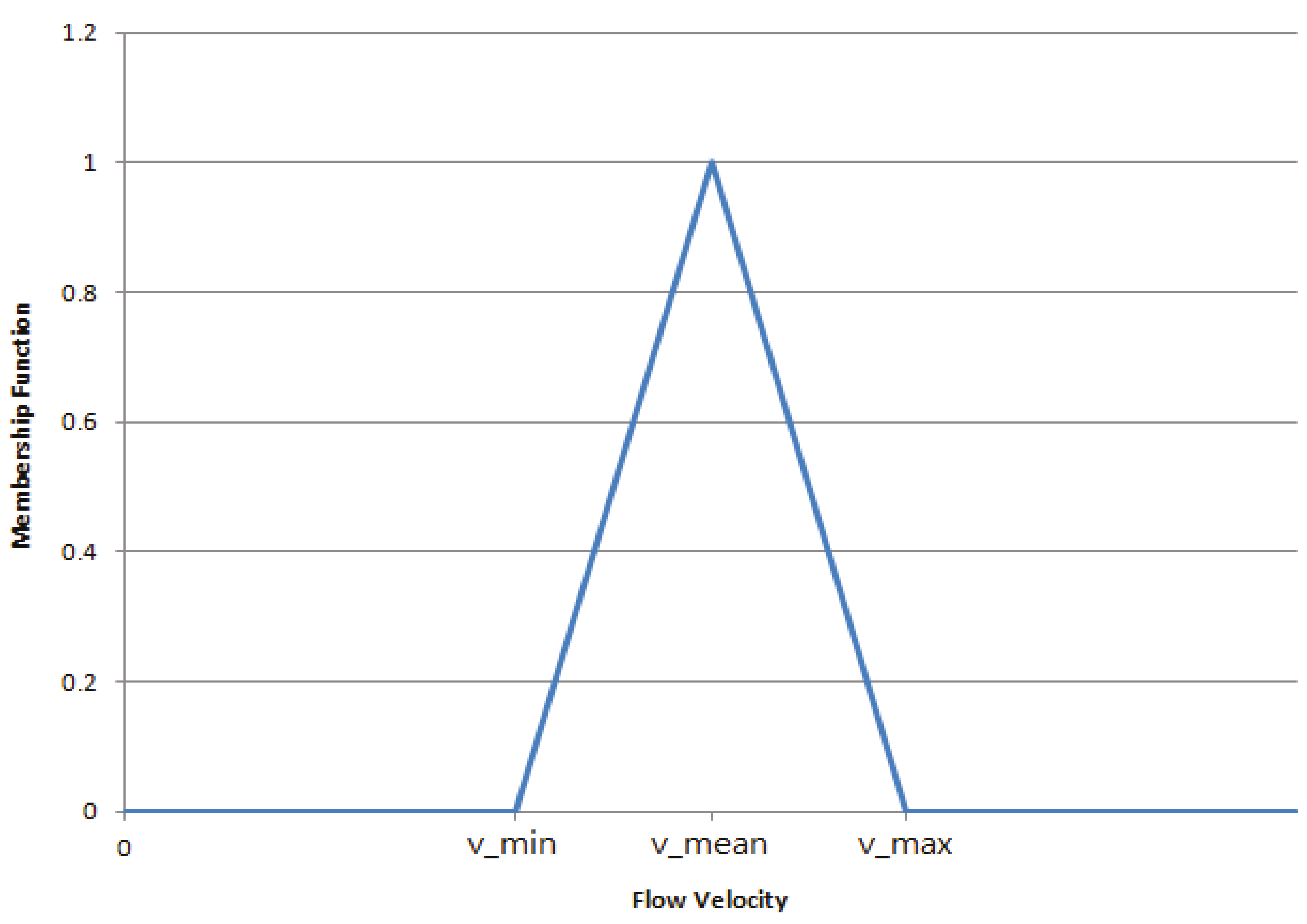
2. Fuzzy Theory and Multi-Objective Function
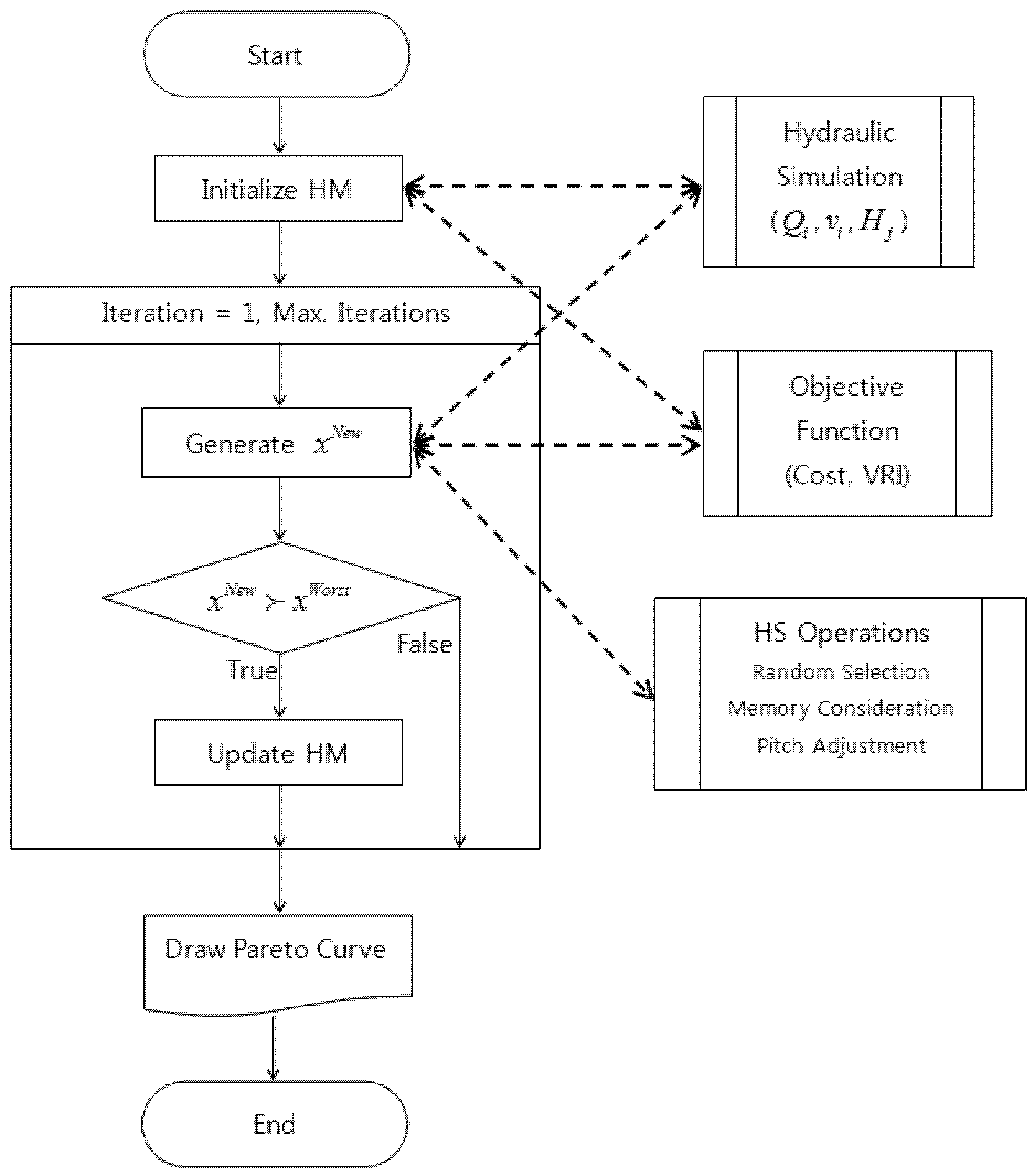
3. Harmony Search Algorithm
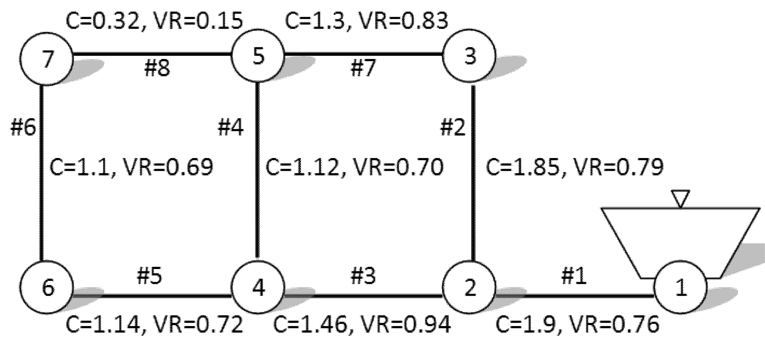
4. Applications and Results


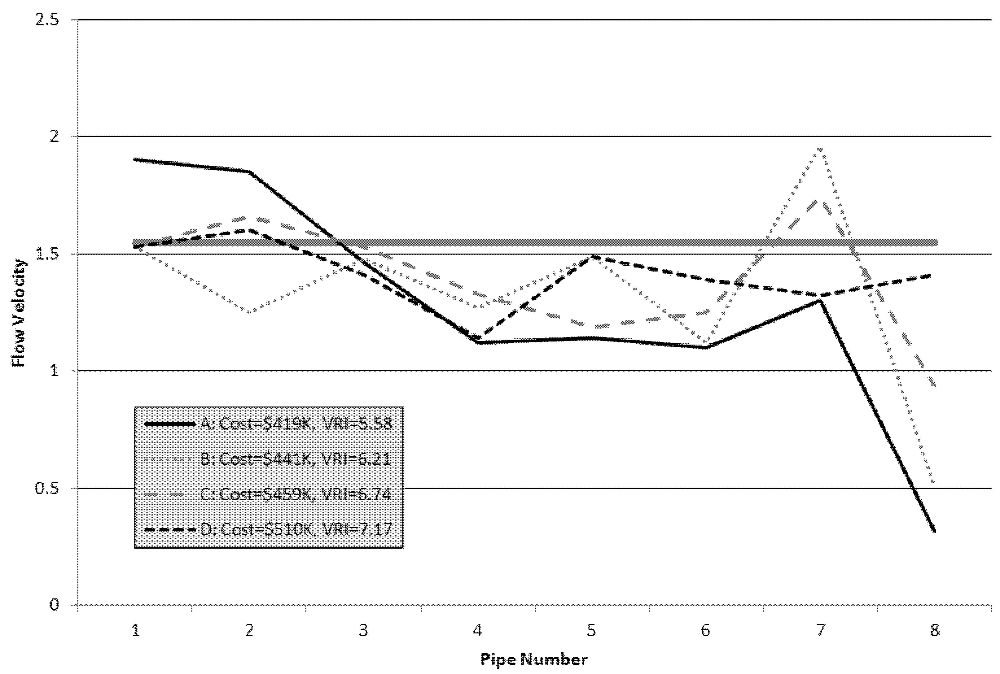
| Pareto Solution (Cost, VRI) | Pipe Diameters (inch) and Velocities (m/s) | |||||||
|---|---|---|---|---|---|---|---|---|
| 1 | 2 | 3 | 4 | 5 | 6 | 7 | 8 | |
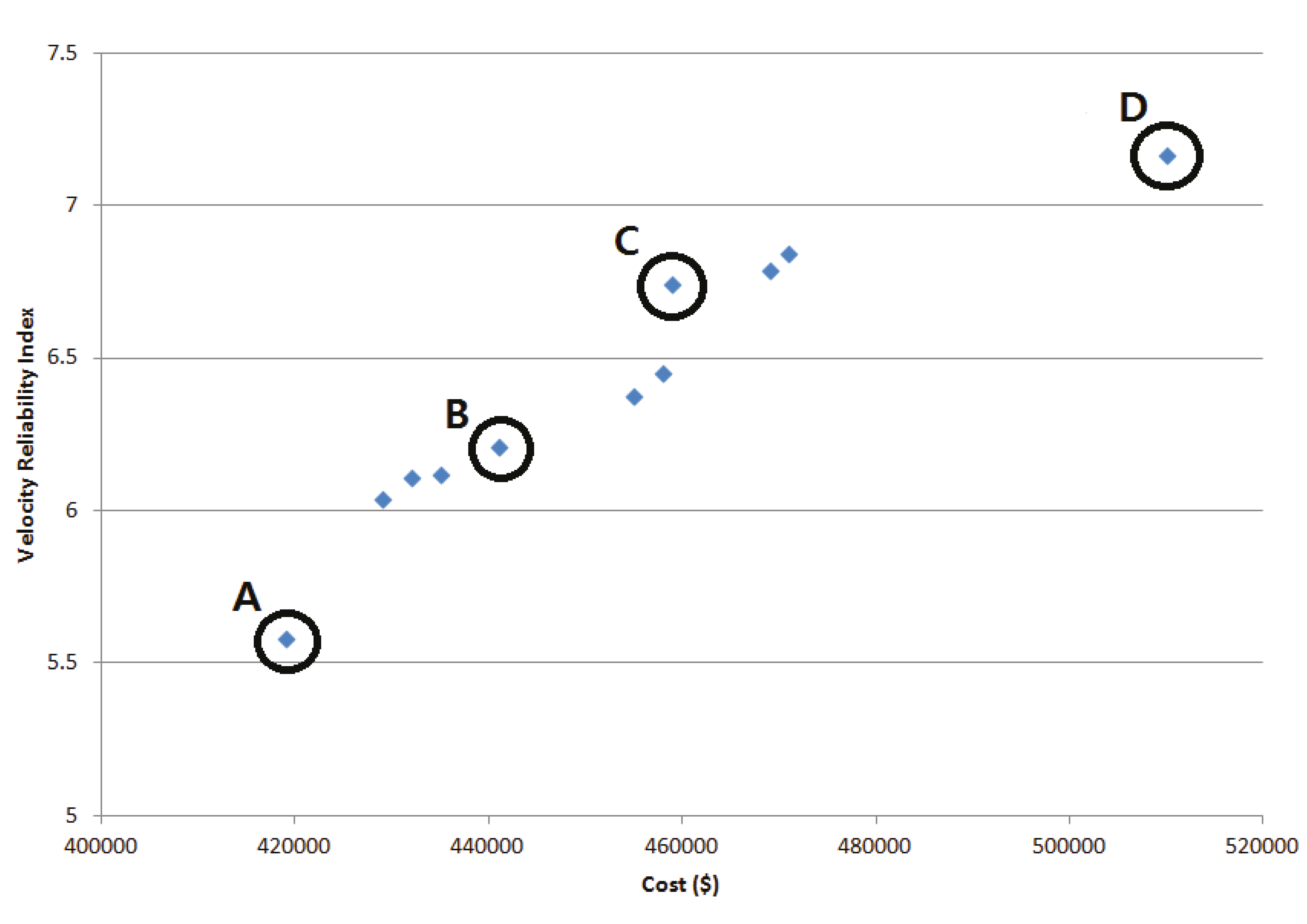
| A ($419 K, 5.58) | 18 (1.9) | 10 (1.85) | 16 (1.46) | 4 (1.12) | 16 (1.14) | 10 (1.1) | 10 (1.3) | 1 (0.32) |
| B ($441 K, 6.21) | 20 (1.53) | 12 (1.25) | 16 (1.48) | 4 (1.27) | 14 (1.49) | 10 (1.12) | 8 (1.96) | 2 (0.51) |
| C ($459 K, 6.74) | 20 (1.53) | 10 (1.66) | 16 (1.53) | 4 (1.33) | 16 (1.25) | 10 (1.25) | 8 (1.74) | 4 (0.94) |
| D ($510 K, 7.17) | 20 (1.53) | 8 (1.6) | 18 (1.41) | 3 (1.14) | 16 (1.49) | 12 (1.39) | 6 (1.32) | 8 (1.41) |

| Pipe Number | Pipe Diameters (mm) | ||||
|---|---|---|---|---|---|
| Solution 1 | Solution 2 | Solution 3 | Solution 4 | Solution 5 | |
| 1 | 400 | 400 | 400 | 400 | 400 |
| 2 | 200 | 200 | 200 | 200 | 200 |
| 3 | 200 | 200 | 200 | 200 | 200 |
| 4 | 200 | 200 | 200 | 200 | 200 |
| 5 | 200 | 200 | 200 | 200 | 200 |
| 6 | 300 | 300 | 300 | 300 | 300 |
| 7 | 200 | 200 | 200 | 200 | 200 |
| 8 | 200 | 200 | 200 | 200 | 200 |
| 9 | 200 | 200 | 200 | 200 | 200 |
| 10 | 300 | 300 | 300 | 300 | 300 |
| 11 | 200 | 250 | 250 | 200 | 200 |
| 12 | 300 | 300 | 250 | 300 | 300 |
| 13 | 200 | 200 | 200 | 200 | 200 |
| 14 | 200 | 200 | 200 | 200 | 200 |
| 15 | 250 | 200 | 200 | 200 | 200 |
| 16 | 200 | 200 | 200 | 200 | 200 |
| 17 | 200 | 200 | 200 | 200 | 200 |
| 18 | 300 | 300 | 300 | 300 | 300 |
| 19 | 300 | 300 | 350 | 350 | 400 |
| 20 | 200 | 200 | 200 | 200 | 200 |
| 21 | 200 | 200 | 200 | 200 | 200 |
| 22 | 300 | 300 | 250 | 300 | 250 |
| 23 | 200 | 200 | 200 | 200 | 200 |
| 24 | 250 | 250 | 250 | 200 | 250 |
| 25 | 200 | 200 | 200 | 200 | 200 |
| 26 | 200 | 200 | 200 | 200 | 200 |
| 27 | 200 | 200 | 200 | 250 | 200 |
| 28 | 200 | 200 | 200 | 200 | 200 |
| 29 | 200 | 200 | 250 | 250 | 250 |
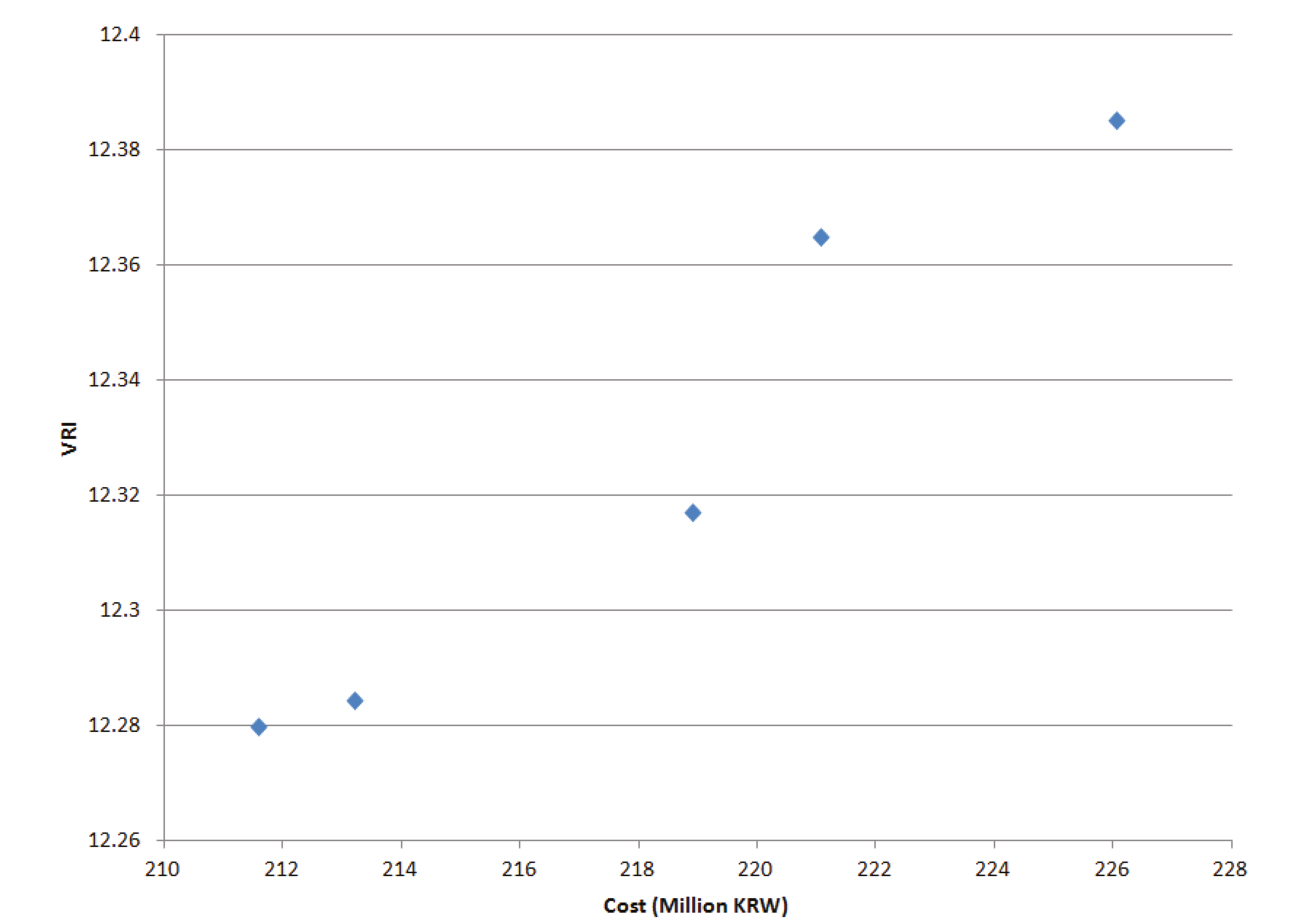
| Design Cost (Korean Won) | 211.6 × 10⁶ | 213.2 × 10⁶ | 218.9 × 10⁶ | 221.1 × 10⁶ | 226.1 × 10⁶ |
| VRI | 12.280 | 12.284 | 12.317 | 12.365 | 12.385 |
5. Conclusions
Conflicts of Interest
References
- Savic, D.A.; Walters, G.A. Genetic algorithms for least-cost design of water distribution networks. J. Water Resour. Plan. Manag. 1997, 123, 67–77. [Google Scholar] [CrossRef]
- Cunha, M.C.; Sousa, J. Water distribution network design optimization: Simulated annealing approach. J. Water Res. Plan. Manag. 1999, 125, 215–221. [Google Scholar] [CrossRef]
- Lippai, I.; Heaney, J.P.; Laguna, M. Robust water system design with commercial intelligent search optimizers. J. Comput. Civil. 1999, 13, 135–143. [Google Scholar] [CrossRef]
- Eusuff, M.; Lansey, K.E. Optimization of water distribution network design using the shuffled frog leaping algorithm. J. Water Res. Plan. Manag. 2003, 129, 210–225. [Google Scholar] [CrossRef]
- Maier, H.R.; Simpson, A.R.; Zecchin, A.C.; Foong, W.K.; Phang, K.Y.; Seah, H.Y.; Tan, C.L. Ant colony optimization for design of water distribution systems. J. Water Resour. Plan. Manag. 2003, 129, 200–209. [Google Scholar] [CrossRef]
- Geem, Z.W. Optimal cost design of water distribution networks using harmony search. Eng. Optim. 2006, 38, 259–280. [Google Scholar] [CrossRef]
- Perelman, L.; Ostfeld, A. An adaptive heuristic cross-entropy algorithm for optimal design of water distribution systems. Eng. Optim. 2007, 39, 413–428. [Google Scholar] [CrossRef]
- Lin, M.-D.; Liub, Y.-H.; Liua, G.-F.; Chua, C.-W. Scatter search heuristic for least-cost design of water distribution networks. Eng. Optim. 2007, 39, 857–876. [Google Scholar] [CrossRef]
- Geem, Z.W. Particle-swarm harmony search for water network design. Eng. Optim. 2009, 41, 297–311. [Google Scholar] [CrossRef]
- Mohan, S.; Jinesh Babu, K.S. Optimal water distribution network design with honey-bee mating optimization. J. Comput. Civil Eng. 2010, 24, 117–126. [Google Scholar] [CrossRef]
- Zheng, F.; Simpson, A.R.; Zecchin, A.C. A decomposition and multi-stage optimization approach applied to optimization of water distribution systems with multiple sources. Water Resour. Res. 2013, 49, 380–399. [Google Scholar] [CrossRef]
- Abebe, A.; Solomatine, D. Application of global optimization to the design of pipe networks. In Proceedings of International Conference on Hydroinformatics, Copenhagen, Denmark, 24–26 August 1998; pp. 989–995.
- Alfonso, L.; Jonoski, A.; Solomatine, D.P. Multiobjective optimization of operational responses for contaminant flushing in water distribution networks. J. Water Res. Plan. Manag. 2010, 136, 48–58. [Google Scholar] [CrossRef]
- Geem, Z.W.; Kim, J.-H.; Jeong, S.-H. Cost efficient and practical design of water supply network using harmony search. Afr. J. Agric. Res. 2011, 6, 3110–3116. [Google Scholar]
- Rossman, L.A. EPANET 2: Users Manual; US Environmental Protection Agency: Cincinnati, OH, USA, 2000. [Google Scholar]
- Samani, H.M.; Mottaghi, A. Optimization of water distribution networks using integer linear programming. J. Hydraul. Eng. 2006, 132, 501–509. [Google Scholar] [CrossRef]
- Walski, T.; Chase, D.V.; Savic, D.; Grayman, W.M.; Beckwith, S.; Koelle, E. Advanced Water Distribution Modeling and Management; Haestead Press: Waterbury, CT, USA, 2003. [Google Scholar]
- Todini, E. Looped water distribution networks design using a resilience index based heuristic approach. Urban Water 2000, 2, 115–122. [Google Scholar] [CrossRef]
- Prasad, T.D.; Park, N.-S. Multiobjective genetic algorithms for design of water distribution networks. J. Water Resour. Plan. Manag. 2004, 130, 73–82. [Google Scholar] [CrossRef]
- Prasad, T.D.; Tanyimboh, T.T. Entropy based design of “Anytown” water distribution network. In Proceedings of Water Distribution Systems Analysis, Kruger National Park, South Africa, 17–20 August 2008; pp. 1–12.
- Ghajarnia, N.; Haddad, O.B.; Mariño, M.A. Reliability based design of water distribution network (WDN) considering the reliability of nodal pressures. In Proceedings of World Environmental and Water Resources Congress, Kansas City, MS, USA, 17–21 May 2009; pp. 1–9.
- Liu, H.X.; Savic, D.; Kapelan, Z.; Zhao, M.; Yuan, Y.X.; Zhao, H.B. A diameter-sensitive flow entropy method for reliability consideration in water distribution system design. Water Resour. Res. 2014, 50, 5597–5610. [Google Scholar] [CrossRef]
- Atkinson, S.; Farmani, R.; Memon, F.A.; Butler, D. Reliability indicators for water distribution system design: Comparison. J. Water Res. Plan. Manag. 2014, 140, 160–168. [Google Scholar] [CrossRef]
- Awumah, K.; Goulter, I.; Bhatt, S. Assessment of reliability in water distribution networks using entropy based measures. Stoch. Hydrol. Hydraul. 1990, 4, 309–320. [Google Scholar] [CrossRef]
- Tanyimboh, T.T.; Templeman, A.B. Calculating maximum entropy flows in networks. J. Oper. Res. Soc. 1993, 44, 383–396. [Google Scholar] [CrossRef]
- Farmani, R.; Walters, G.A.; Savic, D.A. Trade-off between total cost and reliability for anytown water distribution network. J. Water Res. Plan. Manag. 2005, 131, 161–171. [Google Scholar] [CrossRef]
- Di Nardo, A.; Greco, R.; Santonastaso, G.F.; Di Natale, M. Resilience and entropy indices for water supply network sectorization in district meter areas. In Proceedings of the 9th International Conference on Hydroinformatics, Tianjing, China, 7–11 September 2010.
- Raad, D.N.; Sinske, A.N.; Van Vuuren, J.H. Comparison of four reliability surrogate measures for water distribution systems design. Water Resour. Res. 2010, 46, W05524. [Google Scholar] [CrossRef]
- Geem, Z.W.; Kim, J.H.; Loganathan, G.V. A new heuristic optimization algorithm: Harmony search. Simulation 2001, 76, 60–68. [Google Scholar] [CrossRef]
- Saka, M.P. Optimum geometry design of geodesic domes using harmony search algorithm. Adv. Struct. Eng. 2007, 10, 595–606. [Google Scholar] [CrossRef]
- Cheng, Y.M.; Li, L.; Lansivaara, T.; Chi, S.C.; Sun, Y. J. An improved harmony search minimization algorithm using different slip surface generation methods for slope stability analysis. Eng. Optim. 2008, 40, 95–115. [Google Scholar] [CrossRef]
- Mun, S.; Geem, Z.W. Determination of viscoelastic and damage properties of hot mix asphalt concrete using a harmony search algorithm. Mech. Mater. 2009, 41, 339–353. [Google Scholar] [CrossRef]
- Ayvaz, M.T. Application of harmony search algorithm to the solution of groundwater management models. Advanc. Water Res. 2009, 32, 916–924. [Google Scholar] [CrossRef]
- Geem, Z.W. Multiobjective optimization of time-cost trade-off using harmony search. J. Constr. Eng. Manag. 2010, 136, 711–716. [Google Scholar] [CrossRef]
- Geem, Z.W. Novel derivative of harmony search algorithm for discrete design variables. Appl. Math. Comput. 2008, 199, 223–230. [Google Scholar] [CrossRef]
- Geem, Z.W.; Sim, K.-B. Parameter-setting-free harmony search algorithm. Appl. Math. Comput. 2010, 217, 3881–3889. [Google Scholar] [CrossRef]
- Hasancebi, O.; Erdal, F.; Saka, M.P. Adaptive harmony search method for structural optimization. J. Struct. Eng. 2010, 136, 419–431. [Google Scholar] [CrossRef]
- Geem, Z.W.; Cho, Y.-H. Optimal design of water distribution networks using parameter-setting-free harmony search for two major parameters. J. Water Res. Plan. Manag. 2011, 137, 377–380. [Google Scholar] [CrossRef]
- Alperovits, E.; Shamir, U. Design of optimal water distribution systems. Water Resour. Res. 1977, 13, 885–900. [Google Scholar] [CrossRef]
- Lay-Ekuakille, A.; Vendramin, G.; Trotta, A. Spirometric measurement post-processing: Expiration data recovery. Sens. J. IEEE 2010, 10, 25–33. [Google Scholar] [CrossRef]
- Lay-Ekuakille, A.; Trotta, A. Processing stabilometric data for electronic knee: Training and calibration. In Proceedings of IEEE Instrumentation and Measurement Technology Conference, Austin, TX, USA, 3–6 May 2010; pp. 882–885.
© 2015 by the authors; licensee MDPI, Basel, Switzerland. This article is an open access article distributed under the terms and conditions of the Creative Commons Attribution license (http://creativecommons.org/licenses/by/4.0/).
Share and Cite
Geem, Z.W. Multiobjective Optimization of Water Distribution Networks Using Fuzzy Theory and Harmony Search. Water 2015, 7, 3613-3625. https://doi.org/10.3390/w7073613
Geem ZW. Multiobjective Optimization of Water Distribution Networks Using Fuzzy Theory and Harmony Search. Water. 2015; 7(7):3613-3625. https://doi.org/10.3390/w7073613
Chicago/Turabian StyleGeem, Zong Woo. 2015. "Multiobjective Optimization of Water Distribution Networks Using Fuzzy Theory and Harmony Search" Water 7, no. 7: 3613-3625. https://doi.org/10.3390/w7073613