Modeling Flood Hazard Zones at the Sub-District Level with the Rational Model Integrated with GIS and Remote Sensing Approaches

Abstract

Robust risk assessment requires accurate flood intensity area mapping to allow for the identification of populations and elements at risk. However, available flood maps in West Africa lack spatial variability while global datasets have resolutions too coarse to be relevant for local scale risk assessment. Consequently, local disaster managers are forced to use traditional methods such as watermarks on buildings and media reports to identify flood hazard areas. In this study, remote sensing and Geographic Information System (GIS) techniques were combined with hydrological and statistical models to delineate the spatial limits of flood hazard zones in selected communities in Ghana, Burkina Faso and Benin. The approach involves estimating peak runoff concentrations at different elevations and then applying statistical methods to develop a Flood Hazard Index (FHI). Results show that about half of the study areas fall into high intensity flood zones. Empirical validation using statistical confusion matrix and the principles of Participatory GIS show that flood hazard areas could be mapped at an accuracy ranging from 77% to 81%. This was supported with local expert knowledge which accurately classified 79% of communities deemed to be highly susceptible to flood hazard. The results will assist disaster managers to reduce the risk to flood disasters at the community level where risk outcomes are first materialized.

1. Introduction

West Africa is prone to frequent floods and droughts due to high variability in rainfall patterns [1]. In the last three decades, the sub-region has witnessed a dramatic increase in flood events, with severe impacts on livelihoods, food security and ecological systems [2,3,4]. Above normal rainfall amounts at the peak of the rainy season in the Sudanian and Sahelian regions (i.e., July to September) frequently lead to severe floods, and cause many of the major rivers (e.g., Niger, Volta river systems, Senegal) to overflow their banks. In 2007, for example, a series of anomalous abundant rainfall events caused severe floods in West Africa (WA) and other parts of Sub-Saharan Africa (SSA) which affected more than 1.5 million people and resulted in the destruction of farm lands, loss of personal effects, destruction of infrastructure, outbreak of epidemic diseases and the loss of human lives [2,4,5,6,7]. Similar floods in 2009 affected an estimated 940,000 people across twelve countries in West Africa, killing about 193 people and destroying properties worth $152 million [8]. In northern Ghana, the impacts of these floods were exacerbated by the spillage of the Bagre dam in neighboring Burkina Faso [2,9]. In 2012, flooding along the river Niger, which is the principal river in West Africa, resulted in the death of 81 and 137 people in Niger and Nigeria, respectively, while displacing more than 600,000 people [10].

Considering the fact that in this region a temperature of 3–6 °C above the late 20th century baseline has a “very likely” prediction and the fact that the projection is expected to occur one or two decades earlier in West Africa than at the global time, West Africa has been described as a hotspot of climate change [11]. The frequency of occurrence of extreme events is expected to increase [12]. There is also medium confidence that projected increase in extreme rainfall will “contribute to increases in rain-generated local flooding” [13], p. 24. This situation will have dire consequences for the sub-region’s agricultural sector and food security [14].

Despite the major impact of floods on the livelihoods of the people living in this region, no attempt has been made to delineate the boundaries of flood intensity at the community level and to identify areas most at risk of flooding. Mapping flood hazard zones is an important first step in the proper management of future flooding events. Flood hazard maps depict areas (extent and depth) that may be at risk of flooding under extreme rainfall conditions (e.g., above normal rainfall). These maps have proven useful around the world, especially in the developed countries [15] and have: (a) assisted in the early identification of populations and elements at risk; (b) served as a guide in spatial planning in order to avoid development in flood prone areas [16,17]; (c) served as information base for implementation of a flood insurance scheme [18] and (d) raised awareness among the public concerning flood prone areas [15].

The use of flood hazard maps for managing disasters in West Africa is virtually non-existent. Disaster managers have for many years relied on traditional methods such as watermarks on buildings, local knowledge and media reports to identify possible affected areas during flood events [19]. Lack of proper records on historical flood events, coupled with logistical and financial challenges have often resulted in a poor preparedness and response to flooding events. Consequently, fatalities have often been high [4,6].

In order to improve this situation, non-governmental organizations (NGOs) and other international bodies have, in recent years, introduced various initiatives, including flood hazard mapping, aimed at improving disaster management in the sub-region. For example, the World Health Organization (WHO) has produced flood hazard maps at national scale for most countries in SSA [20]. Other initiatives have also produced climate change hot spot maps at national, continental and global scales [21,22,23,24], that show regions that are particularly vulnerable to current and future climate change impacts. However, these products suffer the limitation that they are only useful at the national, continental or global scales, and, thus, are of limited use and applicability at the local scale (e.g., district or community level) where small settlements are mostly the worst affected flood areas. Some researchers have reported the use of seasonal climate forecasts by international bodies (e.g., Red Cross and Red Crescent Society) to manage disasters in the sub-region [3]. However, these forecasts are limited to specific years, and are unable to provide information on specific geographical locations that may be at risk of flooding. Other papers reviewed the vulnerability of some West African cities (e.g., Bobo-Dioulasso, Burkina Faso and Saint-Louis, Senegal) in the light of climate change [25], but made no efforts at mapping the spatial limits of the flood risk areas.

Development of flood hazard maps at the local level/scale (e.g., sub-district and community) can achieve a better targeting of rural communities that are vulnerable to floods than the national/global maps that currently exist. Unfortunately, local level flood hazard maps are rare in the Sudanian Savanna of West Africa. Some of the few that exist also lack the needed spatial variability (i.e., within the unit of mapping) required for an effective management of flood events. For example, in Ghana, Forkuo, [9] integrated topographical, land cover and demographic data to derive a composite flood hazard index for all the districts (second administrative unit) in the Northern region of Ghana. The assignment of a composite flood index to each district greatly limits the use of these maps for identifying communities in the district that may be at risk of flooding. Recently, the Environmental Protection Agency (EPA) of Ghana, with the support of the United Nations Development Programs (UNDP) and the African Adaptation Program (AAP) have conducted flood risk mapping for five, out of the two hundred and sixteen, districts in Ghana [26]. They integrated GIS layers of elevation, soil, rainfall, land use and proximity to water bodies to map flood risk areas in the five districts. Although this initiative produced high resolution flood hazard maps for the selected districts, it is extremely limited in extent (i.e., number of districts considered).

Moreover, many flood modeling approaches require complex calibration procedures and demand huge data as inputs, making them unsuitable in data scarce environments such as WA. There remains therefore an urgent need to explore appropriate methodologies that are able to provide the spatial variability at community level and yet yields accurate results with limited data availability.

In this study, an innovative approach involving the use of a simple hydrological model suitable for data scarce environments and integrated with statistical procedures in a GIS environment is proposed to map the spatial limits of flood hazard zones at a high spatial resolution. A unique approach is also proposed to use a bottom-up participatory method based on the principles of Participatory Geographic Information System (PGIS) [27,28,29] and coupled with robust empirical methods to evaluate the results of the modeling procedure. The main motivation was to develop community level flood hazard maps at a fine spatial resolution that could allow for accurate delineation of flood hot spots and flood safe havens at the sub district/community levels in Ghana, Burkina Faso and Benin.

2. Contexts

Within the framework of the WASCAL project, three study areas in three West African countries have been selected. These areas are (i) the Vea in the Upper East region of Ghana (ii) the Dano in the province of Sud-Ouest of Burkina Faso and (iii) the Dassari in the Commune of Materi in North West Benin. These study areas, which belong to the Sudanian Savanna ecological zone, have a similar climate and are under varying forms of agricultural systems. The areas are predominantly rural and have relatively high population density. In addition to differences in geopolitical contexts, the countries were selected because: (i) The entire area fall in the West Sudanian Savanna Ecological Zone, an area with a high agricultural production potential, but also noted for high climate variability and uncertainty; (ii) Relatively good records of existing long-term historical socio-economic data; and (iii) they have experienced more than one natural disaster over the last 10 to 15 years [30].

To be able to identify the spatial extent of high and low flood hazard zones, the three focal sites were delineated to sub-catchments in a GIS environment. There are a number of approaches used to delineate an area into sub- catchments based on a digital elevation model (DEM). In an urban landscape, artificial drainage channels may be used in addition to natural water bodies in delineating the boundaries of the various catchments in an area. This method works relatively well in drainage areas where the slope of the landscape is primarily responsible for the path taken by runoff [19,31]. However, very often in a highly urbanized setting, control structures such as culverts and detention basins can control the boundaries of various sub-catchments [32].

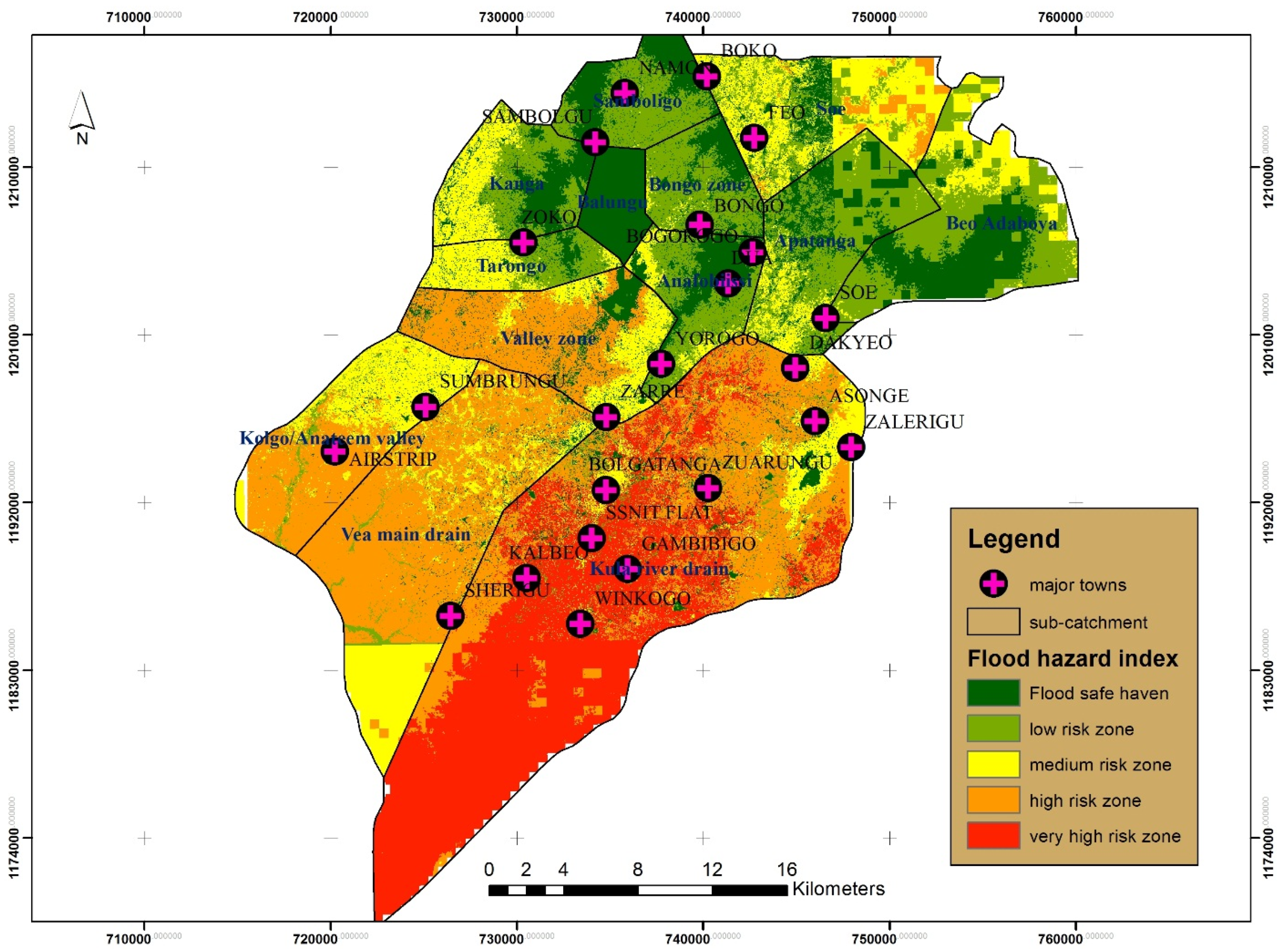
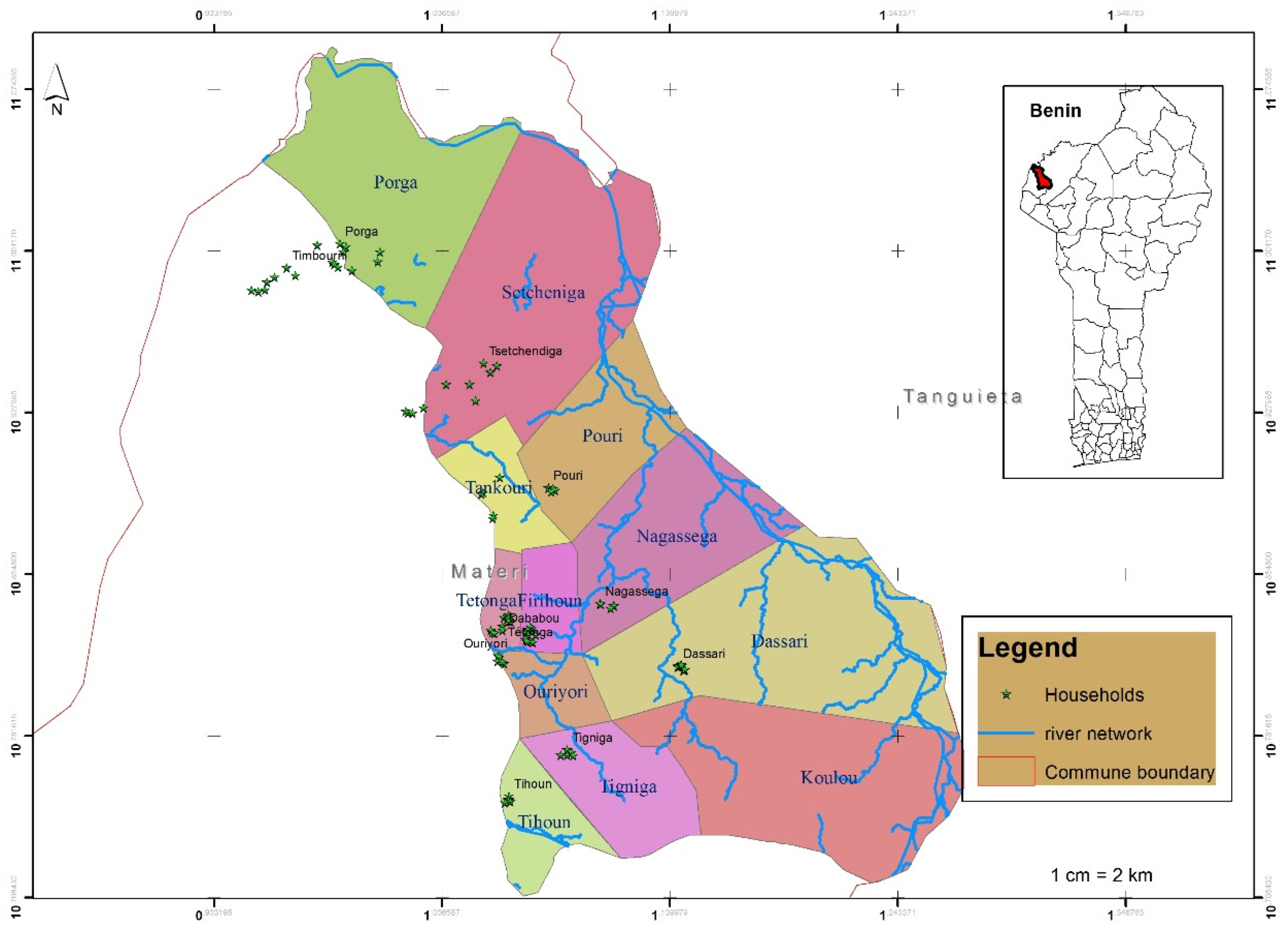
In this study, the delineation into sub-catchments was based on DEM, river channel systems, populations in the communities as well as the operational plans which are used by local disaster managers to segregate and demarcate the areas for effective disaster management. Using this approach, the Vea study area was delineated into 13 sub-catchments. The largest of this sub-catchment is the Kula River drain (Figure 1), named after the Kula river which is well known for causing many of the floods in the area. Other prominent sub-catchments are the Vea main drain and Kolgo/Anateem valley. These sub-catchments are located at the downstream of the Vea and Kolgo Rivers and are also significantly exposed to floods. Similarly, the Dano study area has further been delimited into thirteen sub-catchments in relation to population, contours and river network. The Yo, Bolembar, Gnikpiere and Loffing-Yabogane sub-catchments are prominent among them with extensive river system, smallholder agriculture and many scattered settlements and hamlets. The Dassari area in Benin was also delineated into twelve (12) sub-catchments to reflect population, river network and local administrative structure. The Setcheniga, Porga and Nagassega sub-catchments are most prominent as they are run through by a major river network that significantly exposes the area to flooding. The size of the sub-catchment largely influences the volume of runoff past the outlet hence the larger the catchment size, the greater the potential amount of rainfall that can be captured and directed towards the catchment’s outlet [33]. The sections below provide a brief overview of each of the study areas.

Figure 1. The Vea study area of Ghana.

Figure 1. The Vea study area of Ghana.

2.1. The Vea Study Area

The Vea area (Figure 1) cuts across two districts in Ghana (second administrative units)—Bolgatanga and Bongo—and covers an area of 1037.8 km². The city of Bolgatanga, the capital of Upper East region is found in this area. This study site is the most urbanized of the three study areas and has well developed road network, schools, market access, hospitals, irrigation dams and electricity. Consequently, it has a relatively higher population density of about 104 persons per km². Hydrologically, it falls within the White Volta sub-basin, which extends from northern Ghana to mid Burkina Faso.

The area ranks high amongst areas most exposed to risks from multiple natural hazards occasioned by climate variability. Similar to other parts of West Africa, studies have shown that this area experiences high variability in climate and hydrological flows [34,35]. According to Oduro-Afriyie [36], the area has frequently experienced floods in the past. Between 1991 and 2013, the area has experienced eight major floods; the largest number of people affected being in 1991 [37]. From 2007 to 2013, there have been consecutive flood events in the area.

In 2007, floods followed immediately after a long period of drought and damaged the initial cereal harvest. During this flood disaster, at least 20 people died and an estimated 400,000 people were affected, over 90,000 people were displaced and nearly 20,000 homes were damaged [5]. The long-term and economic impacts on the northern regional economy are still not known but the World Bank [35] estimated the damage to be around US$130 million. Ghana’s National Disaster Management Organization (NADMO) reports that within a period of three years (2010 to 2012), a total of 702,204 people have been affected by floods in Northern Ghana, of which 42% are in the Upper East region where the Vea study area is located. Within this same period, floods have killed 145 people, destroyed 72,391 houses and inundated 31,263.84 hectares of cropland. Of the 20,403 people affected by floods in the Upper East region in 2011, more than 54% were from the Bolgatanga and Bongo districts and virtually all the 3428 houses that collapsed during this flood event were from the two districts that make up the study area.

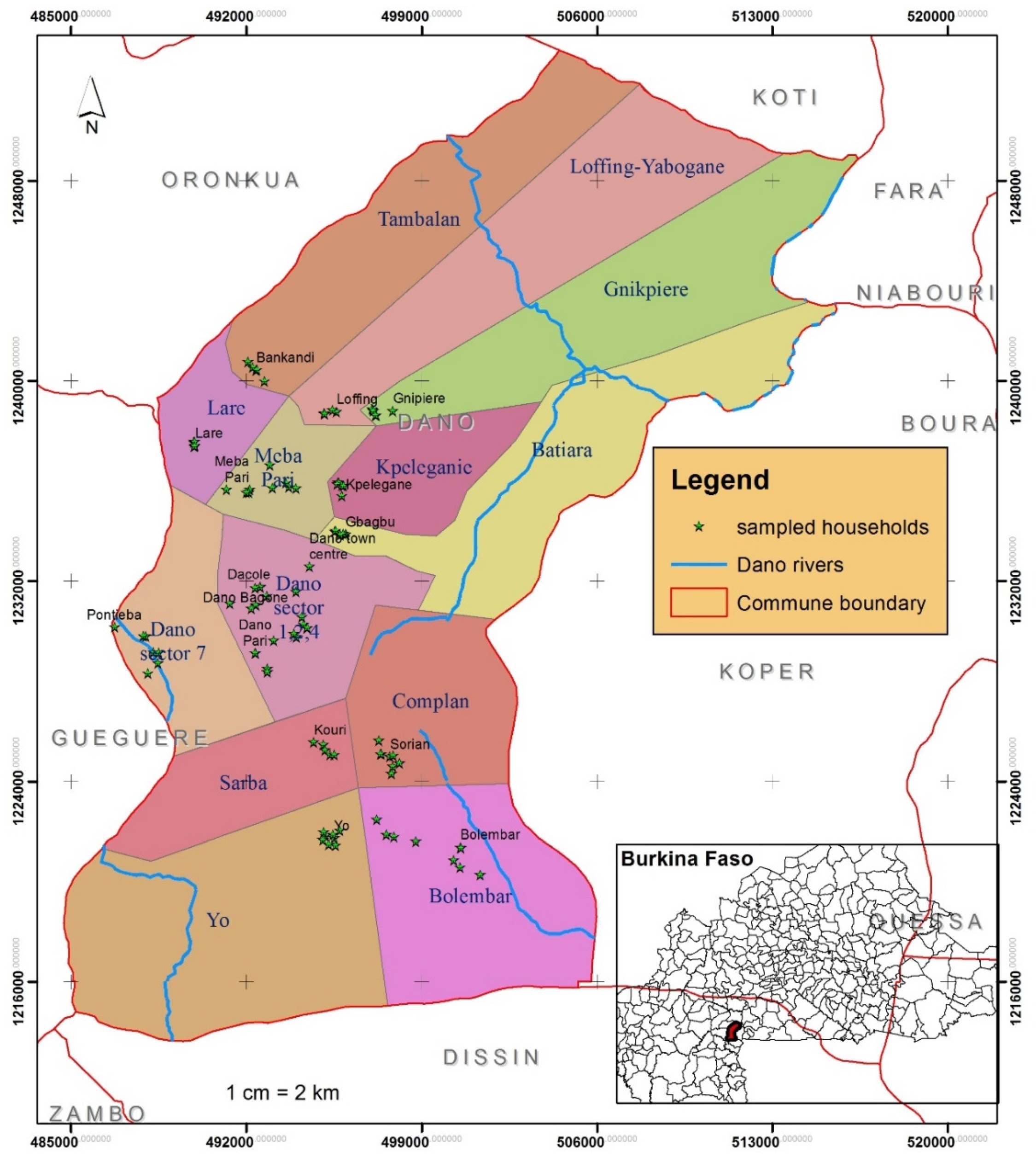
2.2. The Dano Study Area

The Dano study area (Figure 2) is essentially the third sub- administrative level in the province of Ioba of Burkina Faso and has an area of 633.8 km². Population density in this study area is about 59 persons per km². Hydrologically, it falls within the Black Volta sub-basin system, which forms the western part of the Volta basin.

Figure 2. The Dano study area of Burkina Faso.

Figure 2. The Dano study area of Burkina Faso.

Compared to the Vea study area, local scale data on flood hazards in this area is limited. However, available records suggest that in 2009 heavy rains in Burkina Faso caused flooding in many parts of the country and forced officials to open the main gate of a hydroelectric dam (Bagre dam) which also caused flooding in downstream areas in northern Ghana [38]. During this flood, Burkina’s main hospital was closed down. Whereas annual rainfall in Burkina Faso has been averaging 1200 mm, as much as 300 mm occurred within one hour on 1 September 2009 and the Burkinabe Government estimated that it was going to cost US$152 million to face the consequences of the flooding. The Dano study area has severely been affected by floods from torrential rains. In 2008, 410 people were affected, another 720 inhabitants in 2012. The floods in 2010 in particular affected 12 other provinces where more than 160,000 people were directly affected by floods and 14 people were reported dead. Villages were devastated with damage to shelters, livestock, properties, agricultural fields, roads and wells [39]. The occurrence of flood in the area has been increasing in recent years. Field observation show that most houses are easily damaged by flash floods caused by torrential rains. This phenomenon is a great source of worry for many households who already are faced with daunting climate variability issues, low coping and adaptive capacities and thus are highly vulnerable to extreme events.

2.3. The Dassari Study Area

The Dassari study area (Figure 3), which covers an area of 657.1 km², falls in the third sub-national administrative level in Benin (known as the Arrondissement of Dassari) and has a population density of about 56 persons per km². In terms of hydrology, the study area falls within the Oti sub-basin of the Volta basin. The north-eastern corner of the study area forms part of the Pendjari national park in West Africa.

Figure 3. The Dassari study area of Benin.

Figure 3. The Dassari study area of Benin.

At the national level, the worst flood in Benin since 1963 occurred in September 2010 when heavy downpour and influx from the Niger River flooded 55 out of the 77 municipalities in the country including the Materi commune where this study area is located. In this flood alone, over 680,000 people were affected, 800 cases of cholera were reported, 55,000 homes were destroyed and at least 56 people were killed [40].

Similar to Dano, there is limited local scale data available on flood hazards in this study area. However, available data suggest the area has also not been spared of the hydrological hazards that have plagued the other two study areas. Similar catastrophic events were reported in 2008, 2011 and 2012 in the Dassari study area. The 2011 floods in particular resulted in heavy damages to poultry and livestock and thousands of hectares of farmland. In 2013, the local agricultural department had to distribute seeds to over 3600 farmers in the study area to replant about 223 hectares which had been destroyed by floods in the previous farming season.

3. Methods

3.1. Overview of Flood Hazard Mapping

Development of flood hazard maps has often been through the integration of spatial layers representing flood causal factors (e.g., elevation, runoff, land use, etc.) in a Geographic Information System (GIS) environment [15,19]. In recent years, and with the advancement of satellite technology, a number of studies have explored the use of satellite images and GIS in developing flood hazard maps [9,31,41]. Morjani, [20] reviewed four major techniques for developing flood maps. These techniques include hydrological frequency analysis, hydraulic modeling, hydrological models and statistical methods.

• In Hydrologic frequency analysis, historical flood data is used to estimate the probability and spatial extent of future floods events for different time intervals [42,43]. The reliance of this method on historical data limits its usefulness because physical parameters that existed when the floods occurred will no longer remain the same for future floods [20].
• A hydraulic model such as the Engineering Center’s River Analysis System (HEC-RAS) developed by the Hydrologic Engineering Center (HEC) of the US Army Corps of Engineers (USACE) estimates inundation extent, duration and changes in water depth and velocity using river steady flow measurements [44,45]. This model produces highly accurate results for small catchments. However, it requires significant amounts of input such as high resolution Digital Elevation Models (DEMs), stream network model and detailed cross-sectional geometries of river channels.
• In hydrological models, mathematical estimation procedures use a known or an assumed value for components of the hydrological cycle to model stream flow behavior in specific study areas. There are two derivates of hydrological models. These are deterministic models that are based on physical parameters and processes whilst stochastic model allow for the probabilistic variability in both parameters and processes [19,46,47,48,49].
• The last method used in determining flood prone areas is the statistical method which combines historical flood frequency and associated causal factors to estimate flooded areas. This method allows for the derivation of Flood Hazard Index (FHI) as applied in Islam and Sado [41] and Morjani [20].

The first two of the flood modeling approaches reviewed above require complex calibration procedures and demand large data inputs, making them unsuitable in data scarce environments like West Africa. In this study, the last two approaches were integrated with GIS and remote sensing techniques to develop a Flood Hazard Index at the community level.

3.2. Integration of Hydrological and Statistical Models in GIS

In this study, two flood modeling approaches—hydrological model and statistical procedures—were combined to map the spatial extent of flood hazard areas at a high spatial resolution at sub district level. First, a modified version of the rational hydrological model [47,49] was used to estimate the runoff of the respective catchments based on rainfall intensity, the area of LULC type within catchments and a runoff coefficient. Thereafter, statistical procedures were adopted in a GIS environment to integrate the output of the hydrological model with other flood causal factors such as topography (DEM) to determine a flood hazard intensity map for the respective study areas. Flood hazard zones were eventually defined through a reclassification of the flood hazard intensity maps to derive the Flood Hazard Index (FHI) which determines the flood hazard zones of an area.

Morjani [20] found that the use of statistical procedures in mapping flood hazards zones resulted in the following benefits: (a) there are reliable estimates of flood hazard zones because the integration of the statistical methods avoids the use of a purely empirical model; (b) There is ease of integration in Geographic Information System (GIS); (c) is able to consider both the susceptibility of each small area to be inundated and flood emergency management. This could allow for delineating flood hazard zones at community level which then helps local disaster managers to effectively manage local disasters; (d) allows the use of knowledge of flood causal factors which are readily available from local experts.

The uniqueness of this present study is the integration of the statistical methods which then allows a simple hydrological model to be applied in this data scarce environment. Statistical procedures were used at two different stages. The first stage is where various standardization methods were applied to develop the flood hazard index. The second stage is where statistical procedures were combined with PGIS principles to evaluate the results of the flood maps.

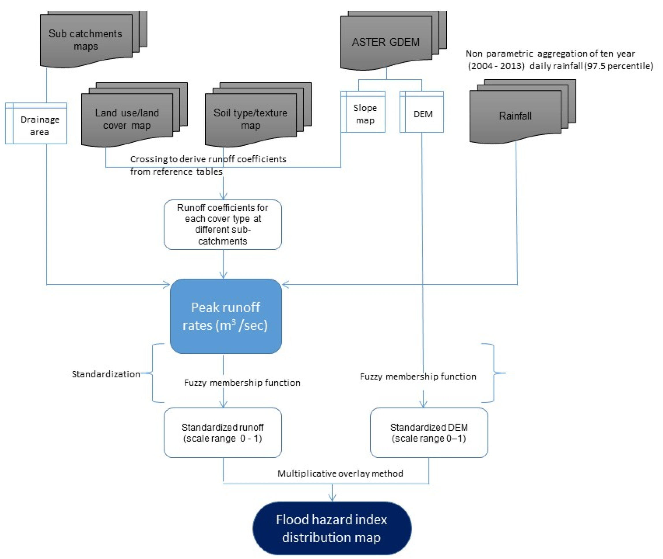
The methodological approach adopted has been diagrammatically summarized in Figure 4.

As first step, the approach retrieves data values from all flood causal factors and then calculates peak runoff rates using the rational model. The causal factors for flood which have been elaborated in section 3.4 are land cover/use, soil type and texture, slope, elevation, rainfall and drainage area [20]. It then uses the statistical procedures to determine the peak runoff rates at different elevations before applying standardization methods to determine flood hazard zones.

Figure 4. Integration of hydrological and statistical models with GIS.

Figure 4. Integration of hydrological and statistical models with GIS.

3.3. Determination of Peak Runoff Using the Rational Model

The rational model [47,49] belongs to the group of lumped hydrological models which treats the unit of analysis (normally a catchment or sub-catchment) as a single element whose hydrological parameters (e.g., rainfall) are considered as average values [50]. The strength of this model lies in its simplicity and the ease of implementation. Consequently, it has been widely used to calculate peak surface runoff rate for the design of a variety of drainage structures [51], study area modeling and flood hazard mapping [19]. The rational model converts rainfall in a catchment into runoff by determining the product of the rainfall intensity in the catchment and its area, reduced by a runoff coefficient (C, between 0 and 1), which is a function of the soil, land cover and slope in the study catchment. The runoff coefficient, which is the most critical parameter in the rational model [52], provides an estimation of how much water (rainfall) is lost due to infiltration (soil), interception and evapotranspiration (land cover). Thus, the runoff coefficient of a catchment can be considered as the fraction of rainfall that actually becomes storm water runoff [51]. Accurate determination of this parameter is, therefore, vital to the successful implementation of this method. The rational model operates on a number of assumptions including:

• The entire unit of analysis is considered as a single unit,
• Rainfall is uniformly distributed over the drainage area.
• predicted peak runoff has the same probability of occurrence (return period) as the used rainfall intensity (I),
• the runoff coefficient (C) is constant during the rain storm

The model is given by the equation:

$${{\displaystyle Q}}_{\text{p}}=0.28\times C\times I\times A$$

(1)

where,

• Q_p = Peak runoff rate (m³/sec)
• C = Runoff coefficient (-)
• I = Rainfall intensity (mm/hr)
• A = Drainage area (Km²)

The factor “0.28” is required to convert the original units in North American system (i.e., cubic feet per second—cfs) to an international system such as cubic meters per second (m³/s).

3.4. Flood Causal Factors and Retrieval Methodologies

In this study, spatial layers of land use and land cover, soil and slope were analyzed to accurately determine the runoff co-efficient prior to the implementation of Equation (1). The sections below (3.4.1 to 3.4.4) details the source or the methodology used to derive each of the four datasets and the preliminary processing conducted on each.

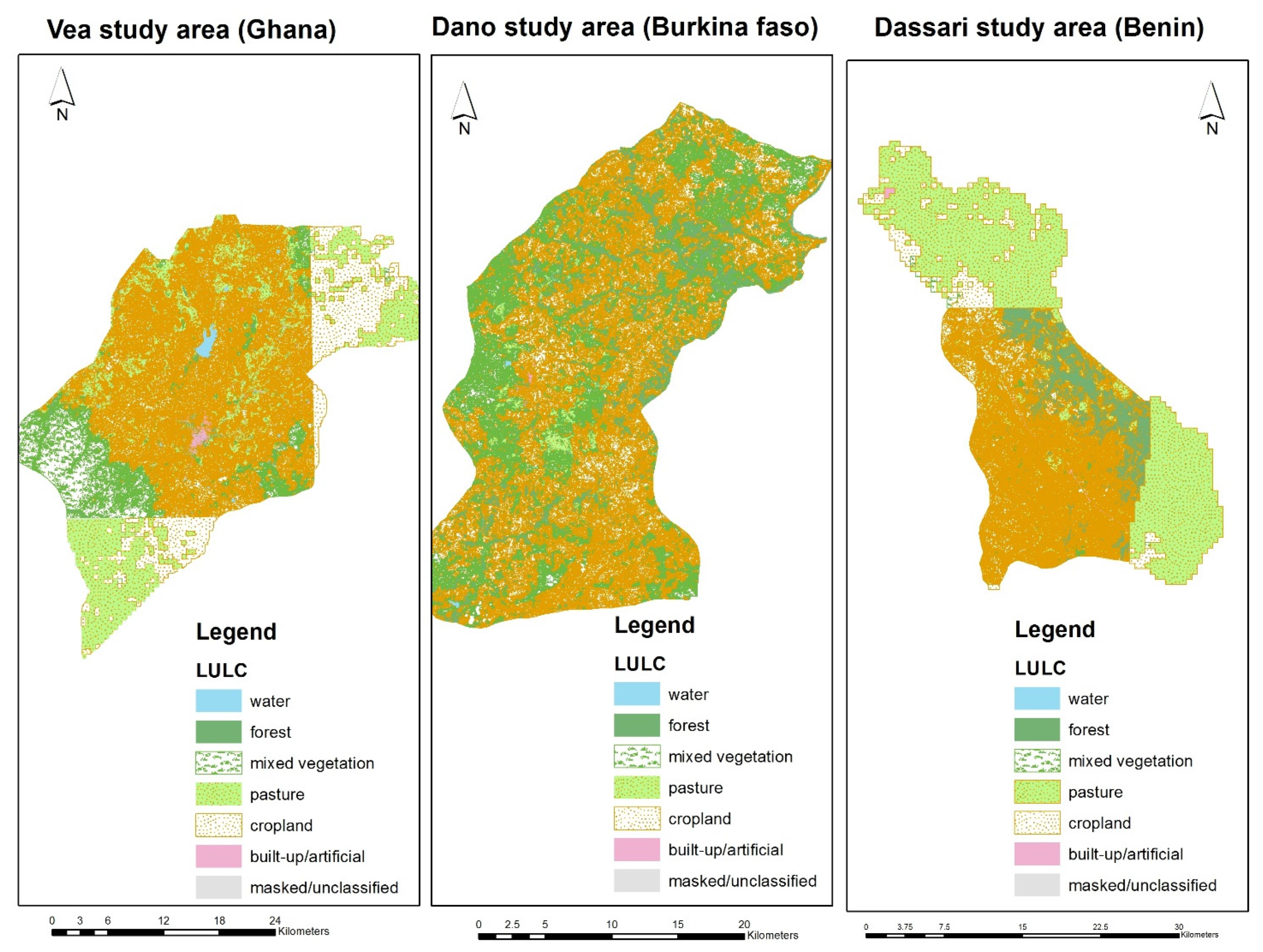
3.4.1. Land Use/Land Cover (LULC)

The type of LULC in an area determines how much rainfall infiltrates the soil and how much becomes runoff. Impervious surfaces such as concretes have runoff coefficients approaching one while surfaces with vegetation to intercept rainfall and promote water infiltration have lower runoff coefficients [51,53]. There is a direct relationship between land cover and hydrological parameters of interception, infiltration, runoff and concentration which ultimately influence flooding [19,41,54,55,56].

In this study, LULC maps for the three study areas were generated by classifying high spatial resolution (5 m) multi-temporal RapidEye images acquired between April and November 2013 [57,58]. RapidEye provides data in five spectral channels (blue, green, red, red edge and near infrared). Table 1 provides details of the images analyzed and their acquisition dates.

Table 1. Satellite imagery used and their acquisition dates.

Study Area	Satellite Data Used	Acquisition Dates (DD/MM/2013)
Vea	RapidEye	01/04; 02/05; 03/06; 19/09; 02/10; 03/11
	TerraSAR-X	25/09; 21/10
Dano	RapidEye	01/04; 03/05; 30/09; 13/10
	TerraSAR-X	30/07; 10/08; 12/09; 15/10
	Landsat	12/06; 14/07; 03/11
Dassari	RapidEye	04/04; 02/05; 13/06; 19/09; 12/10; 15/11
	TerraSAR-X	15/05; 17/06; 20/07; 22/08

Table 1. Satellite imagery used and their acquisition dates.

Study Area	Satellite Data Used	Acquisition Dates (DD/MM/2013)
Vea	RapidEye	01/04; 02/05; 03/06; 19/09; 02/10; 03/11
	TerraSAR-X	25/09; 21/10
Dano	RapidEye	01/04; 03/05; 30/09; 13/10
	TerraSAR-X	30/07; 10/08; 12/09; 15/10
	Landsat	12/06; 14/07; 03/11
Dassari	RapidEye	04/04; 02/05; 13/06; 19/09; 12/10; 15/11
	TerraSAR-X	15/05; 17/06; 20/07; 22/08

The images were atmospherically corrected with ENVI ATCOR2 [59] prior to analysis. Classification was conducted to reveal five broad LULC classes. These are: (1) croplands (all crop classes); (2) forest (trees with a crown canopy of greater than 70%); (3) grasslands; (4) mixed vegetation (combination of grassland, herbs and shrubs) and (5) artificial surfaces (buildings, bare areas, tarred roads, etc.). Training and validation data for these classes were obtained from field campaigns conducted between July and October 2013. Training and validation samples for the classification were generated by overlaying the training and validation data (polygons) on the time-series satellite images and extracting the corresponding values.

The Random Forest (RF) classification algorithm [60] as implemented in the R statistical software [61] was used to classify the images of the respective study areas. RF generates a large set of independent classification trees, each trained on a bootstrapped sample (randomly selected) of the training samples. The training samples consist of a matrix of rows and columns, where the columns (also called predictors or variables) represent the individual spectral bands of the underlying image, while each row represents the corresponding values of a pixel in the spectral bands. RF’s construction of a large number of classification trees overcomes the limitation of single decision trees, which often over fit the training data [62]. Each classification results were independently validated with the validation samples. Overall classification accuracies of 88%, 95% and 97% were obtained for the Dano, Vea and Dassari catchments respectively.

As indicated in the introductory section, this study explores appropriate methods to map flood hazard at community level in the face of a daunting challenge relating to limited data availability. One effect of scarce data is on the images analyzed. It did not spatially cover the studies areas, particularly the Dassari study area and to some extent the Vea study area. Consequently, a 500 m resolution global LULC map produced from Moderate Resolution Image Spectroradiometer (MODIS)—MCD12Q1 [63] was used to fill-in the areas that were not covered by the RapidEye and TerraSAR-X images. MCD12Q1 products are developed on an annual basis. Thus, to ensure consistency with the LULC map produced in this study, the 2013 version was downloaded and utilized. The MODIS product was resampled to the resolution of the RapidEye and TerraSAR-X images but some variations in spatial resolutions of the LULC can be seen at the affected areas (Figure 5). Figure 5 shows the final LULC maps of the respective watersheds.

3.4.2. Digital Elevation Model (DEM)/Slope

A study area with a greater slope will have more runoff and thus a higher runoff coefficient than a study area with a lower slope, Ceteris Paribus. The probability of a flood increases with decreasing elevation and hence is a strong indicator for flood susceptibility [41,46,64,65,66,67]. The slope angle and topography are important factors of runoff. Probability of flooding increases when slope angle is below a critical value and then decreases logarithmically [26]. In this study, the Advanced Space borne Thermal Emission and Reflection Radiometer (ASTER) Global Digital Elevation Model (GDEM) developed jointly by the Japanese Ministry of Economy, Trade and Industry (METI) and the United States National Aeronautics and Space Administration (NASA) was used to derive the slope maps for the respective study areas. The ASTER GDEM was produced by applying automated procedures to process the entire 1.5-million-scene ASTER archive, including stereo-correlation, cloud masking to remove cloudy pixels, stacking, removal of residuals and outliers, averaging and finally portioning into 1°-by-1° tiles. This ASTER GDEM which has spatial resolution of 1 arc second (approximately 30 m) grid was downloaded in GeoTIFF format from ASTER GDEM Page [68]. The data has a vertical accuracy of 20 m at 95% confidence level [69]. The downloaded DEM was converted to percent slope in a GIS application after all the sinks had been filled to remove small imperfections. In accordance with standardized tables for calculating runoff coefficient, the slope map was reclassified into three classes; (1) areas with slope less than 2%; (2) areas with slope between 2% and 6% and (3) areas with slope greater 6%. Besides the slope map that was obtained, the filled DEM layer was maintained and used later in the integration of peak runoff and elevation to determine runoff concentration at different elevations.

Figure 5. Land Use/Land Cover (LULC) maps of the study areas. MODIS—MCD12Q1 product was used to fill in portions of the high resolution RapidEye and TerraSAR-X images for particularly the Dassari study area and to some extent the Vea study area. As can be seen, the southernmost and north eastern portions of the Vea study area and in the case of Dassari, the north and southeastern portions were the main areas affected. The MODIS product was resampled to the resolution of that of the RapidEye and TerraSAR-X images.

Figure 5. Land Use/Land Cover (LULC) maps of the study areas. MODIS—MCD12Q1 product was used to fill in portions of the high resolution RapidEye and TerraSAR-X images for particularly the Dassari study area and to some extent the Vea study area. As can be seen, the southernmost and north eastern portions of the Vea study area and in the case of Dassari, the north and southeastern portions were the main areas affected. The MODIS product was resampled to the resolution of that of the RapidEye and TerraSAR-X images.

3.4.3. Soil Type and Texture

Soils that have a high clay content do not allow very much infiltration and thus have relatively high runoff coefficients, while soils with high sand content have higher infiltration rates and low runoff coefficients [51,53]. Nyarko [19], Todini et al. [54] found the important role played by soil type in influencing water infiltration, runoff and hence flood susceptibility. The texture of a soil influences its erodability, water retention capacity, crust formation and aggregate stability. The amount of water available for runoff is thus a function also of both soil texture and structure [26]. The Natural Resource Conservation Service of the United States has classified four broad hydrological soil groups that provide useful information in determining study area runoff coefficients. Classification into any of these groups can either be on the basis of a description regarding soil texture or measured infiltration rates [51]. The study used the 1km resolution soil map from the Harmonized World Soil Database (HWSD) version 1.1 produced in 2009 by the International Institute for Applied System Analysis (IIASA). The HWSD is an image file linked to a comprehensive attribute database in Microsoft Access. This attribute information includes soil mapping units, soil texture for top and sub soils and several other soil properties. Details about this database can be found in FAO [70]. Based on the soil texture attribute information, the extracted soil maps of the study areas were reclassified into the four main soil hydrological groups (A to D) defined by the United States Soil Conservation Service [71].

3.4.4. Rainfall

The probability of a flood increases with increasing rainfall within a specified time period [19,20,54]. We obtained daily data of precipitation at a resolution of about 11 × 11 km based on the African Rainfall Climatology, version 2 (ARC2), subsetted to our period of analysis (2004–2013) and study area in West Africa. This period was chosen because of increased occurrence of flood events recorded in the areas as mentioned in Section 2. These data were then further aggregated to capture long-term precipitation magnitude (97.5th percentile, median, and 2.5th percentile) and extremes (97.5th percentile). To capture long-term precipitation magnitude (97.5th percentile, median, and 2.5th percentile) and extremes (97.5th percentile), the time-series of records per grid are statistically considered as a population (rainfall records per grid, 2004–2013). The extreme (97.th percentile) for each grid was retained as input to the calculation of Peak Storm Water Runoff Rate. The rational for this non-parametric aggregation is found in the stochasticity of rainfall; a parametric aggregator (i.e., maximum or mean) would be sensitive to outliers and data errors.

Called the African Rainfall Climatology, version 2 (ARC2), the underlying dataset is a revision of the first version of the ARC [72] consistent with the operational Rainfall Estimation, version 2, algorithm (RFE2), ARC2 uses inputs from two sources:

• Three-hourly geostationary infrared (IR) data centered over Africa from the European Organization for the Exploitation of Meteorological Satellites (EUMETSAT) and
• Quality-controlled Global Telecommunication System (GTS) gauge observations reporting 24-h rainfall accumulations over Africa.

The main difference with ARC1 resides in the recalibration of all Meteosat First Generation (MFG) IR data (1983–2005). Results show that ARC2 is a major improvement over ARC1. It is consistent with other long-term datasets, such as the Global Precipitation Climatology Project (GPCP) and Climate Prediction Center (CPC) Merged Analysis of Precipitation (CMAP), with correlation coefficients of 0.86 over a 27-year period. However, a marginal summery dry bias that occurs over West and East Africa is examined. Daily validation with independent gauge data shows RMSEs of 11.3, 13.4, and 14, respectively, for ARC2, Tropical Rainfall Measuring Mission Multi satellite Precipitation Analysis 3B42, version 6 (3B42v6), and the CPC morphing technique (CMORPH) for the West African summer season. The reconstructed Africa Rainfall Climatology (ARC2) offers a number of advantages compared to other long-term climatological rainfall datasets that are widely used. First, high resolution historical rainfall estimates on a daily basis would help not only to monitor precipitation associated with synoptic and mesoscale disturbances, but also to undertake studies of extreme events, wet and dry spells, number of rain days (i.e., rainfall frequency), and onset of the rainfall seasons. Second, a 0.1° (~11 km) spatial resolution allows users to see rainfall phenomenon on local scales that cannot be captured by coarser climate datasets [72].

3.5. Development of Peak Runoff Maps

Within the study area, more than one land cover type, slope and soil group exists. In order to find representative runoff coefficients within a given land cover, sub-catchment runoff coefficient was determined using the areas of the different LULC type and then the hydrologic soil group, and slope complexes as weighting factors. The classical application of the rational model requires treating the entire sub-catchment as a single unit and thus, does not lead to spatial variability of the runoff and for that matter, flood risk within sub-catchments. In this study, however, a novel technique is introduced where the various classes of LULC types within the sub-catchments are used as the unit of analysis to ensure spatially explicit assessment of flood risk. This was required because the key purpose of this study is to explore methods to derive community level flood risk in a data scarce environment. Therefore, we sought to operationalize the rational model in a way that meets the objective of the study. It was realized that treating the whole sub-catchment as a single unit will not lead to a determination of the spatial variability of discharge within a sub-catchment which is required to understand community level flood risk. Therefore, instead of using the sub-catchment as the unit of analysis (which is the classic application of the rational model), the area of the different landuse units was used as the unit of analysis. In other words, the area of the various LULC classes were computed and peak runoff estimated for each cover type. Although this approach has some limitation especially regarding catchment boundaries where a land use/cover type crosses the boundaries, it was found to be conceptually and operationally better than implementing the rational model in its raw form which can only give single peak runoff for each sub-catchment based on many averages (i.e., average coefficient, rainfall and total area).

A runoff coefficient map was first generated by vectoring the reclassified layers of LULC, slope and soil layers and overlaying them in a GIS. The overlay resulted in multiple polygons each having a unique LULC, soil and slope class. Based on Table 2, which specifies a runoff coefficient for a combination of LULC, soil type and slope, the attribute table of the resultant overlay layer was populated with the corresponding runoff coefficient number. This layer was eventually rasterized (30 m resolution) for subsequent analysis.

In order to allow for integration with the generated runoff coefficient map, the rainfall intensity map was resampled to a cell resolution of 30 m to correspond to the spatial resolution of the ASTER GDEM layer. A vector layer of the sub-catchment map containing the areas (in km²) of each LULC type within each sub-catchment was also rasterized into a 30 m resolution raster. Once the raster layers of the runoff coefficient (C), rainfall intensity (I) and sub-catchment areas (A) was ready, the runoff peak layer was calculated by implementing Equation (1) in a GIS using raster algebra.

Table 2. Rational method runoff coefficients.

LULC	Runoff Coefficient
	Soil Group A			Soil Group B			Soil Group C			Soil Group D
Slope	<2%	2%–6%	>6%	<2%	2%–6%	>6%	<2%	2%–6%	>6%	<2%	2%–6%	>6%
Cropland	0.14	0.18	0.22	0.16	0.21	0.28	0.20	0.25	0.34	0.24	0.29	0.41
Forest	0.08	0.11	0.14	0.10	0.14	0.18	0.12	0.16	0.20	0.15	0.20	0.25
Grassland	0.15	0.25	0.37	0.23	0.34	0.45	0.30	0.42	0.52	0.37	0.50	0.62
Mixed vegetation	0.14	0.22	0.30	0.20	0.28	0.37	0.26	0.35	0.44	0.30	0.40	0.50
Artificial Surfaces	0.33	0.37	0.40	0.35	0.39	0.44	0.38	0.42	0.49	0.41	0.45	0.54

Note: Source: Knox County Tennessee [73].

Table 2. Rational method runoff coefficients.

LULC	Runoff Coefficient
	Soil Group A			Soil Group B			Soil Group C			Soil Group D
Slope	<2%	2%–6%	>6%	<2%	2%–6%	>6%	<2%	2%–6%	>6%	<2%	2%–6%	>6%
Cropland	0.14	0.18	0.22	0.16	0.21	0.28	0.20	0.25	0.34	0.24	0.29	0.41
Forest	0.08	0.11	0.14	0.10	0.14	0.18	0.12	0.16	0.20	0.15	0.20	0.25
Grassland	0.15	0.25	0.37	0.23	0.34	0.45	0.30	0.42	0.52	0.37	0.50	0.62
Mixed vegetation	0.14	0.22	0.30	0.20	0.28	0.37	0.26	0.35	0.44	0.30	0.40	0.50
Artificial Surfaces	0.33	0.37	0.40	0.35	0.39	0.44	0.38	0.42	0.49	0.41	0.45	0.54

Note: Source: Knox County Tennessee [73].

3.6. Statistical Modeling

The generated peak runoff map was combined with the elevation layer to produce the flood hazard intensity map. However, prior to that, the two layers (peak runoff and elevation) were standardized. Due to the dissimilar units (i.e., m³/s for peak runoff and m for elevation), standardization was necessary to make any combination of the two layers meaningful. The fuzzy set theory [74] was used to standardize the layers into comparable scales prior to combining them. Compared to other methods (e.g., Boolean sets) that allow only binary membership functions (i.e., true (1) or false (0)—membership or no membership), the fuzzy set theory admit the possibility of a partial membership [75]. This means that the transition between membership (1) and non-membership (0) of a location in the set is gradual, compared to sharp boundaries, in for example, Boolean sets [74]. Fuzzy sets are, therefore, characterized by a membership grade that ranges from “0” to “1”, indicating a continuous increase from non-membership (0) to complete membership (1).

The fuzzy membership function implemented in ESRI’s ArcGIS was used to standardize the peak runoff and elevation layers. Due to the positive linear relationship between peak runoff and probability of flooding, the peak runoff layer was linearly rescaled between the minimum and maximum values using a linear membership type. This means the lowest peak runoff value in each study area was assigned a value of “0” (i.e., no membership or low probability of flooding) while the highest peak runoff value was assigned a value of “1” (full membership or high probability of flooding), with all other values in-between the two extremes rescaled between “0” and “1”. Thus, the lowest likelihood for a flood to occur in a given sub-catchment was rescaled as 0 with 1 for categories with the highest likelihood. The reverse, however, was done for the elevation layer. Theoretical principle underlying the relationship between elevation and probability of flooding indicate a negative relationship. In other words, areas with low elevation have a higher probability of flooding than areas with high elevation values. Therefore in rescaling the respective elevation layers, the lowest value was assigned a membership of “1” (i.e., high probability of flooding) while the highest value was assigned a membership of ‘0’ (low probability), will all other values in-between rescaled between “0” and “1”.

3.7. Developing Intensity Level of Flood Hazard Distribution Map

The standardized peak runoff and elevation layers were combined using the weighted linear combination method [76] to produce the flood hazard intensity map at different elevations. Equation (2) was implemented in a GIS to achieve this. The method permits the assignment of weights, which indicates the relative importance of a layer. The weights must add up to one. In this study, the two standardized layers were considered equally important, thereby assigning a weight of 0.5 each to the layers in Equation (2).

$$FHI={\displaystyle \sum _{i=1}^n{w}_i{x}_i}\text{ Or more simply as }FHI={\displaystyle \sum _{i=1}^{n}0.5X(DEM)+0.5X(\text{peak runoff})}$$

(2)

where “FHI” is the flood hazard intensity, x_i is the ith standardized layer, w_i is the weight of the ith standardized layer and “n” is the number of standardized layers to be combined.

Since the weights of the respective layers sum up to one, the output from Equation (2) has the same value range (0 to 1) as the standardized layers, where “0” signifies areas with low flood risk while areas with high flood risk are given a value of “1”. For each pixel, this method multiplies the standardized peak runoff score with the score of the standardized DEM to produce the distribution of runoff at different elevations which is indicative of flood hazard. In order to make the map easily understandable, a reclassification was performed to define five flood hazard intensity levels/categories—very low, low, medium, high and very high. The natural breaks reclassification method in ESRI’s ArcGIS was used for this purpose. The natural breaks (jenks) classification algorithm finds data break points between classes depending on the natural patterns in which the data are clustered. Class break points are set where there are relatively huge jumps in the data values.

4 Results and Discussion

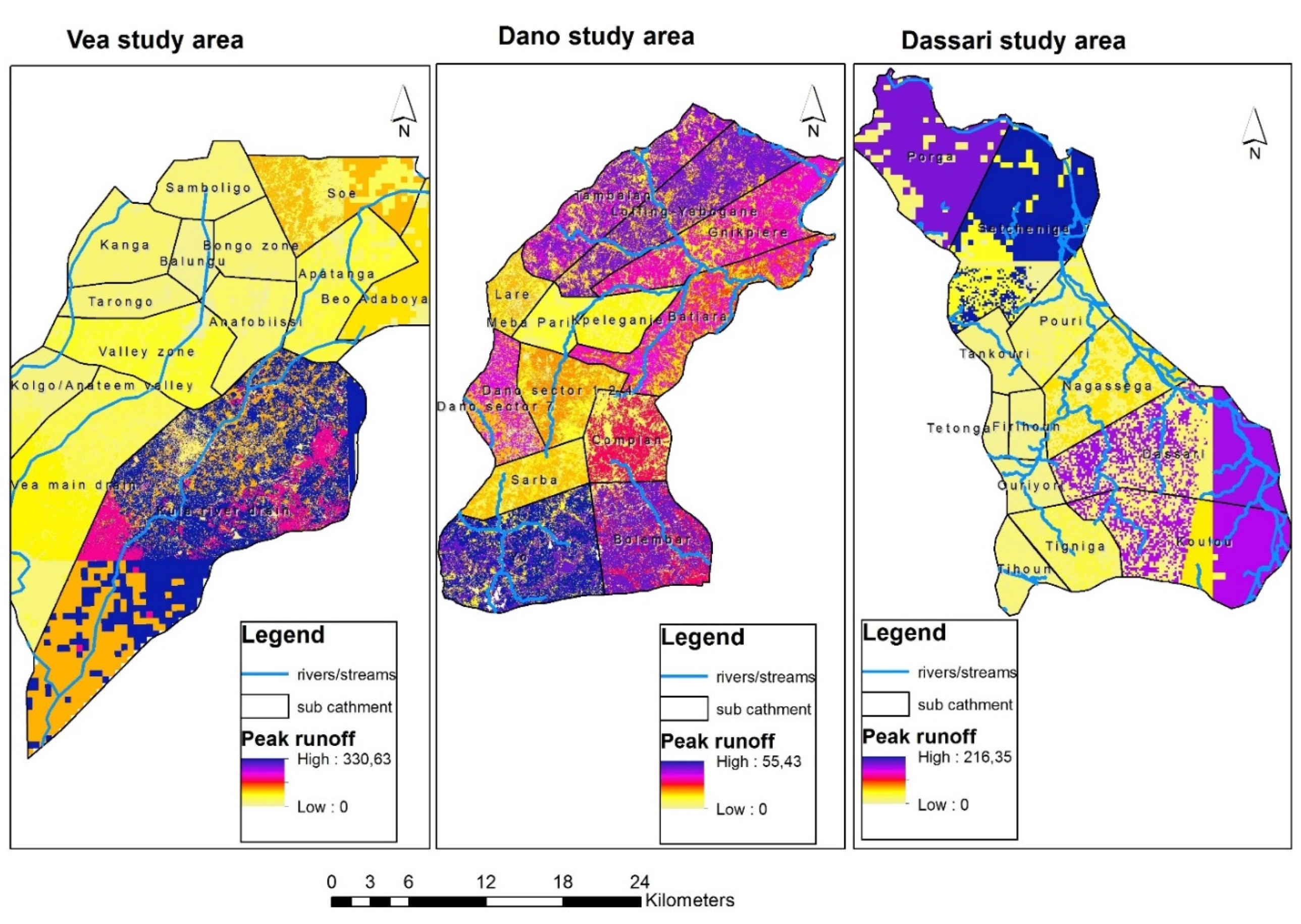
4.1. Peak Runoff Rates

Maps of the peak runoff rates in cubic meters per second (M³/s) have been produced for the three study areas and show the distribution of runoff within all the catchments in the three areas studied. These maps are presented in Figure 6.

Table 3 presents the total amount of peak runoff generated within the various sub-catchments. In the Vea study area, the Kula river sub-catchment generates the highest amount of runoff in excess of 713.0 M³/s whilst the lowest amount was generated in the Balungu sub-catchment with an amount of 26.0 M³/s. In the Dano study area in Burkina Faso, the Yo sub-catchment recorded the highest peak runoff rate of 119.6 M³/s whilst the Meba Pari segment generates a meager 25.5 M³/s. In the Dassari study area in Benin, the Sétchindiga sub-catchment generates the highest amount of 290.5 M³/s as against the lowest amount of 13.6 M³/s generated in the Tetonga sub-catchment.

Comparing the three study areas in the three countries, the Vea study area in Ghana generates an average of 155.7 M³/s per sub-catchment. This amount is higher than the average sub-catchment runoff of 113.11 M³/s in the Dassari study area and 69.0 M³/s in the Dano study area. High runoff is positively correlated with increased susceptibility of flood hazards. As reported in Islam and Sado, [41]; Todini et al. [54]; Bapalu and Sinha [56], there is a direct relationship between hydrological parameters of interception, infiltration, runoff concentration and flooding. Although there is limited data available at the community level in Dano and Dassari study areas, available data collected during the field work shows that the Vea study area record more flood events and more people suffer from flood impacts than both Dano and Dassari study areas. Records from local authorities also show that the Dassari study area also reports more flood events than the Dano study area in conformity with the average runoff figures shown in this study. For instance, between the periods 2008 to 2012, over 294,000 people have been affected by floods in the Vea study area [77] whilst 3600 were affected in the Dassari study area with Dano recording only 1130 people as affected. In addition, whilst the Dassari and Dano study areas have experienced three flood events between 2008 and 2012, there has been consecutive flood event in the Vea study area of Ghana over the same period.

Figure 6. Peak runoff maps of the three study areas.

Figure 6. Peak runoff maps of the three study areas.

Table 3. Results of total amount of peak-runoff generated within the various sub-catchments.

Vea Study Area (Ghana)		Dano Study Area (Burkina Faso)		Dassari Study Area (Benin)
Sub Catchment	Runoff (m3/s)	Sub Catchment	Runoff (m3/s)	Sub Catchment	Runoff (m3/s)
Balungu	26.0	Tambalan	100.3	Dassari	236.8
Beo Adaboya	191.0	Bolembar	86.1	Firihoun	25.8
Bongo zone	68.0	Dano sector 1,2&4	57.0	Nagassega	100.2
Anfobissi	82.4	Batiara	80.8	Ouriyori	27.5
Apatanga	128.6	Gnipiere	88.3	Porga	204.4
Kolgo/Anateem	107.7	Sarba	42.9	Pouri	71.5
Kula river channel	713.2	Kpeleganie	32.6	Sétchindiga Tankouri	290.5
Samboligo	60.3	Lare	34.2	Tetonga	32.1
Soe	201.6	Loffing-Yabogane	112.0	Tigniga	13.6
Valley zone	138.0	Meba Pari	25.5	Tihoun	63.7
Vea main drain	178.0	Dano sector 7	65.1	Koulou	34.0
Tarongo	54.2	Complan	52.2		257.3
Kanga	75.2	Yo	119.6

Table 3. Results of total amount of peak-runoff generated within the various sub-catchments.

Vea Study Area (Ghana)		Dano Study Area (Burkina Faso)		Dassari Study Area (Benin)
Sub Catchment	Runoff (m3/s)	Sub Catchment	Runoff (m3/s)	Sub Catchment	Runoff (m3/s)
Balungu	26.0	Tambalan	100.3	Dassari	236.8
Beo Adaboya	191.0	Bolembar	86.1	Firihoun	25.8
Bongo zone	68.0	Dano sector 1,2&4	57.0	Nagassega	100.2
Anfobissi	82.4	Batiara	80.8	Ouriyori	27.5
Apatanga	128.6	Gnipiere	88.3	Porga	204.4
Kolgo/Anateem	107.7	Sarba	42.9	Pouri	71.5
Kula river channel	713.2	Kpeleganie	32.6	Sétchindiga Tankouri	290.5
Samboligo	60.3	Lare	34.2	Tetonga	32.1
Soe	201.6	Loffing-Yabogane	112.0	Tigniga	13.6
Valley zone	138.0	Meba Pari	25.5	Tihoun	63.7
Vea main drain	178.0	Dano sector 7	65.1	Koulou	34.0
Tarongo	54.2	Complan	52.2		257.3
Kanga	75.2	Yo	119.6

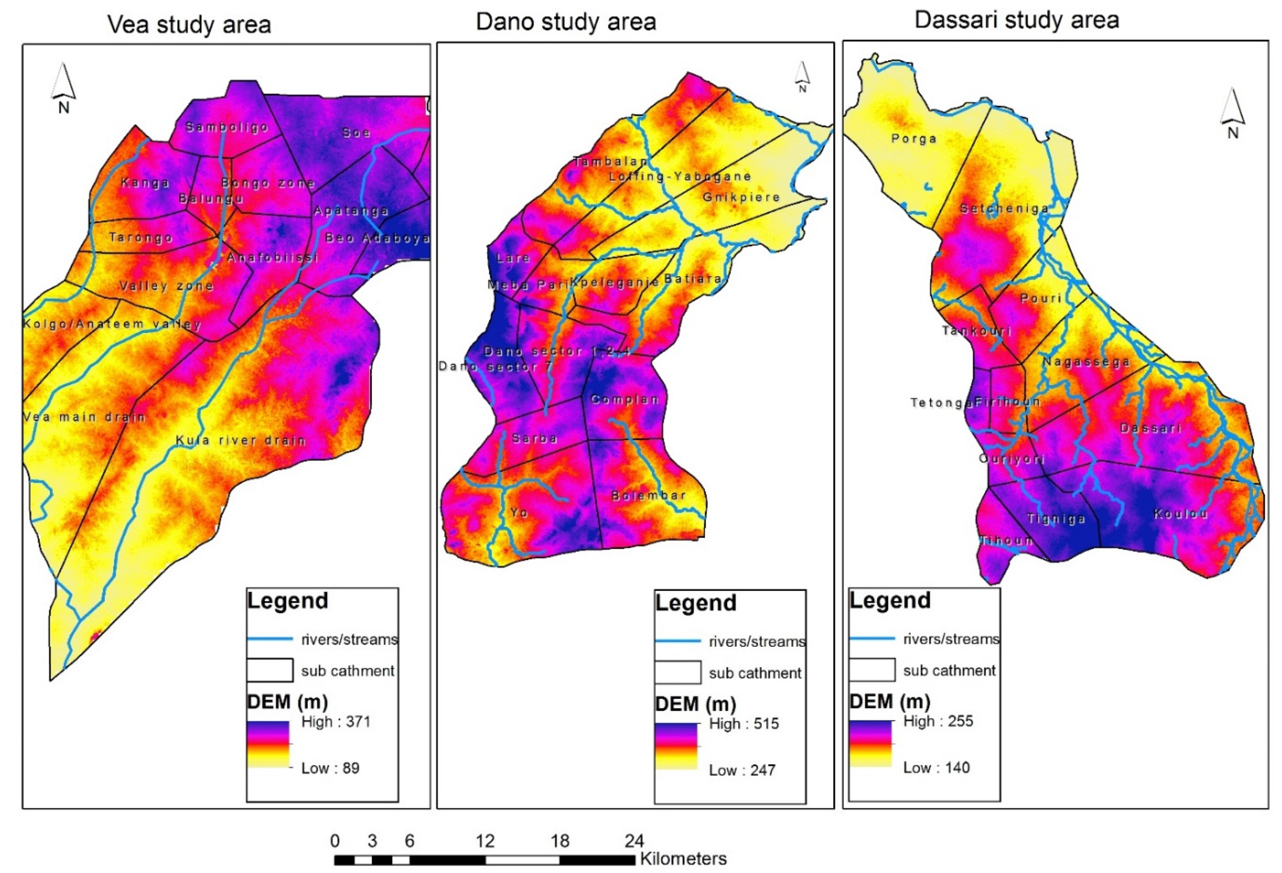
4.2. Digital Elevation Model (DEM)

The map presented in Figure 7 show the DEM of the three study areas. In the Vea study area, high elevations values are concentrated in the Apatanga, Soe, Beo Adaboya and parts of Samboligo sub-catchments whilst the Kula River, Vea main drain and Kolga Anateem valley records very low elevation. Indeed in the southernmost part of the Kula River, a low elevation of 89 m is found. From the peak runoff map, the Kula river sub-catchment simultaneously records high runoff generation.

Figure 7. Digital Elevation Model (DEM) of the study areas.

Figure 7. Digital Elevation Model (DEM) of the study areas.

This area is therefore expected to fall in the category of high flood intensity zone) in the Flood hazard Index (FHI).

In the Dano study area, high elevations values are found in Dano, Sarba and parts of Yo sub-catchments. In this study area, low elevation areas are found in the north-eastern part and largely correspond to the river networks in the area. These areas also generate significant amounts of runoff as can be seen in the maps. In the Dassari study area, high elevation values are found in the southern parts of Tigniga, Tihoun, Koulou, parts of Dassari and Ouriyori sub-catchments. Similar to the Vea study area and Dano study areas, areas in Dassari with low elevation values and hence high risk areas for flooding also correspond to areas generating the largest amounts of runoff. These areas are the Sétchindiga and Porga sub-catchments and are thus expected to result in high flood risk zone.

Comparing the elevation maps of the three study areas, the Vea and Dassari study areas are generally more low-lying than the Dano study area in Burkina Faso. Average elevation in Vea is 196 m as against 379 m in Dano and 197.5 m in Dassari. This fact coupled with relatively high amounts of runoff generation will thus make the Vea more prone to flooding than the other two study areas.

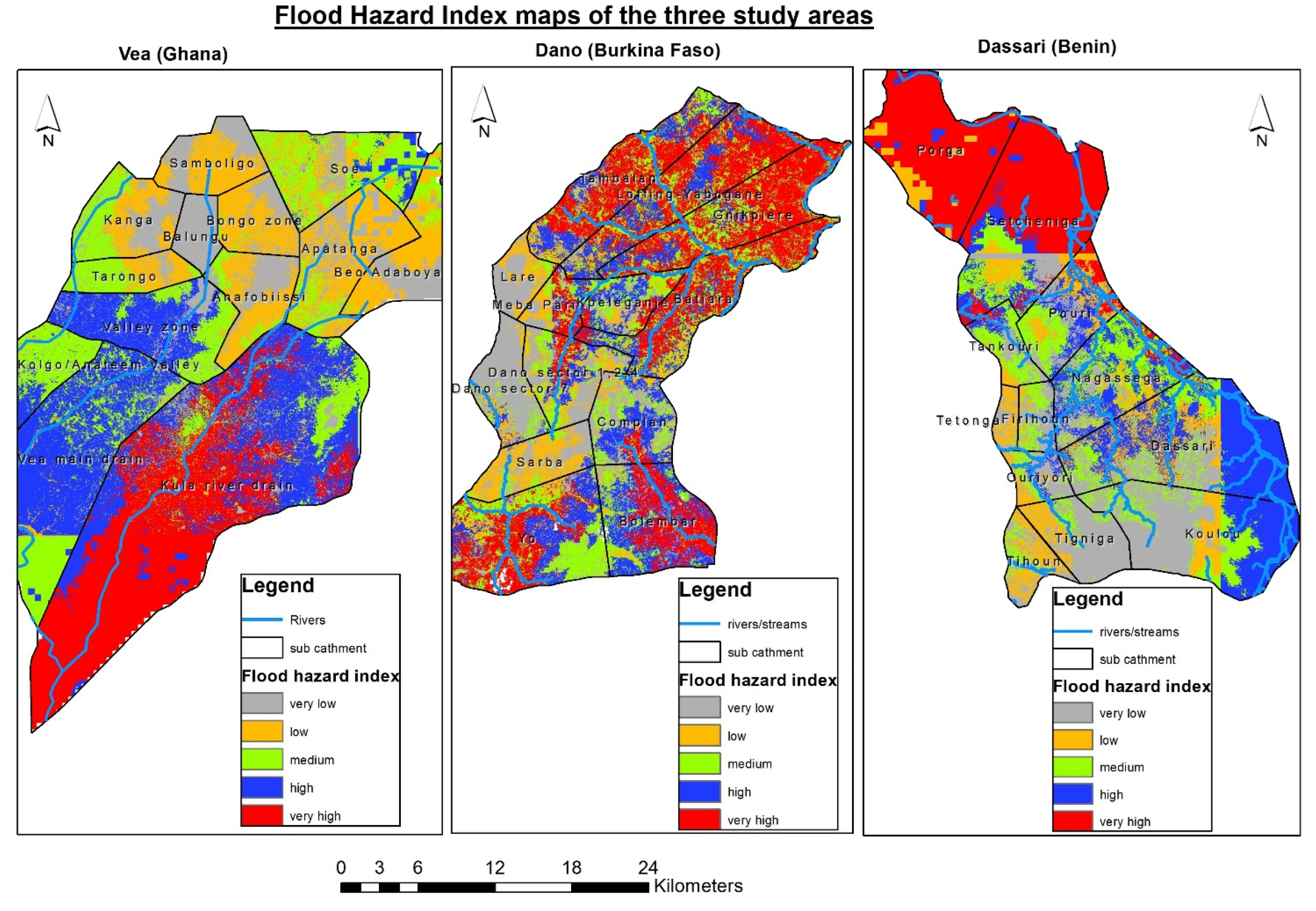
4.3. Flood Hazard Intensity Levels and Flood Hazard Index

By combining the standardized peak runoff maps with the standardized DEM, the flood hazard intensity map was produced. This map was then classified using the Natural Break (Jenks) method into five classes to produce the Flood Hazard Index (FHI). The index ranges from 1 (very low flood hazard intensity) to 5 (very high flood hazard intensity). In Figure 8 below, the final Flood Hazard Index is represented in a graduated colour map.

Figure 8. Flood hazard index.

Figure 8. Flood hazard index.

Figure 8 presents the flood hazard intensity maps of the respective study areas. In the Vea study area of Ghana, the very high flood hazard intensity zone is concentrated in the Kula river sub-catchment. As indicated in Section 4.1 and Section 4.2, this sub-catchment has the highest runoff of 330 M³/s and also has the lowest elevation of 89 m. Consequently, more than half of the sub-catchment falls into the very high flood hazard zone. This sub-catchment has the highest population density. The capital of the Upper East region, Bolgatanga, is found in this sub-catchment and it is the most urbanized and with good infrastructure. Records from the National Disaster Management Organization (NADMO) show that of the 702,000 people affected by floods in northern Ghana between 2010 and 2012, as much as 42% were from the Bolgatanga municipality [77]. This result of the Kula river sub-catchment having the highest flood risk correlates with the modeling result of Ghana’s Water Research Institute [78] when it was found that up to 75 cm of runoff is added to the maximum water level at Pwalugu, an area at the southernmost part of the sub-catchment.

In addition, the Kolga Anateem valley and Vea main drain sub-catchments are found in the high flood hazard intensity zones. With the exception of the valley sub-catchment in Bongo district, none of the sub-catchments in Bongo are located in the very high flood intensity zone. However, there are pockets of high flood hazard intensity zones in the Soe sub-catchment. Almost all of Balungu and parts of Samboligo and Beo Adaboya sub-catchments fall in the very low flood intensity zone and are thus expected to pose no flood risk.

In the Dano study area, very high and high intensity flood hazard zones are distributed throughout the study area. However, the sub-catchments of Yo, Bolembar, Gnipiere, Loffing-Yabogana and Tambalan have significant areas classified as very high flood risk zones. Contrary to the Vea study area, the most populous area in this study area fall into the very low to medium flood hazard intensity zones. Therefore, the Dano township, the capital of the province with a projected population of 20,786 in 2010 [79] largely falls into low flood risk zone.

In the Dassari study area, two sub-catchments stand out in terms of flood risk. The Porga and Sétchindiga sub-catchments have very high flood hazard intensity. This is as a result of low elevation values coinciding with high runoff generation as explained in Section 4.1 and Section 4.2. In addition, in this study area, significant parts of Koulou and Dassari fall in the high flood intensity zone. There are also pockets of high flood intensity zones in Nagessega, Ouriyori, Firihoun and Tetonga sub-catchments.

From Table 4, more than half of the Dano study area (52.1%) falls in the two high flood hazard intensity zones of very high and high. In addition, in the Vea and Dassari study areas, almost half of the entire study areas fall into the very high and high flood risk zone. It must be noted that, the data ranges for the FHI differ among all the study areas but they can all be translated into the five qualitative classification scheme of very high (5), high (4), medium (3), low (2) and very low (1). This is the same procedure adopted by Beck et al. [80] and Birkmann et al. [22] in the World Risk Reports. In addition, important to note is that an area classified as very low flood hazard intensity in the Vea study area could be rendered a high risk due to cross scale interactions. Flood risks from outside the sub-catchment area could lead to cascading hazards. For example, some of the flood events recorded in the Vea study area is as a result of the opening of the Bagre dam in nearby Burkina Faso.

Table 4. Proportions of areas under various flood intensity zones.

Flood Hazard Intensity Number	Flood Hazard Intensity Zone/Class	Percent of Study Area
		Vea	Dano	Dassari
1	Very low	15.2	16.4	23.2
2	Low	18.8	11.2	13.3
3	Medium	19.5	20.3	16.7
4	High	28.2	18.1	22.1
5	Very high	18.42	34.0	24.7
Total High and Very High Risk Zone		46.6	52.1	46.8

Table 4. Proportions of areas under various flood intensity zones.

Flood Hazard Intensity Number	Flood Hazard Intensity Zone/Class	Percent of Study Area
		Vea	Dano	Dassari
1	Very low	15.2	16.4	23.2
2	Low	18.8	11.2	13.3
3	Medium	19.5	20.3	16.7
4	High	28.2	18.1	22.1
5	Very high	18.42	34.0	24.7
Total High and Very High Risk Zone		46.6	52.1	46.8

These cascaded flood events are independent or partially independent of local rainfall in the Vea area and conditions of other flood causal factors. The implication is that an area classified as low or medium flood intensity zone in the Vea as a result of the interactions of the factors considered in this paper could still experience significant flood episodes whenever overflow upstream in the Bagre dam is allowed to pass. At the same time, however, whenever this cross scale influence coincides with high episodes of local rainfall anomalies, sub-catchments such as the Kula River which is already classified as very high flood intensity could experience catastrophic flood event. This is absolutely important for local disaster managers in the Vea area to constantly monitor the operations of dams upstream so as to prevent or minimize the impacts of this knock-on effect.

The study found most of the high flood hazard risk areas close to the major rivers in the area. This was the case in Kula River sub-catchment in Vea, Porga and Sétchindiga in Dassari as well as Yo, Gnikpiere etc. in the Dano study area. This finding is contrary to the assertion by Forkuo [9] that high hazard zones are not necessarily located very near to river bodies.

4.4. Quantitative Validation of the Flood Hazard Index with PGIS and Confusion Matrix

The study introduced an innovative method of applying the principles of Participatory GIS (PGIS) to evaluate the flood map. The approach involves using local disaster managers, community leaders and local disaster volunteers to undertake field evaluation of the five flood categories. The team randomly visited known locations over 5 days in the Vea study area and 3 days in the Dano study area. At each location visited, the local experts were asked to classify the spot into the five flood hazard classes based on their knowledge of flood intensity at that particular location. A GPS receiver was then used to record the geographic coordinates of the location and its attributes. The objective was to construct a confusion matrix which will then allow for the quantitative validation of the flood map using statistical procedures.

Typically, the confusion matrix [81,82,83] is used to display class membership of observations according to the map and according to field observations. The diagonal of the confusion matrix lists the correct classifications while off diagonal cells list errors. The overall accuracy quantifies the proportion of correctly classified pixels. Using this approach, the flood hazard of the Vea and Dano study areas have an overall accuracy of 77.62% and 81.41% respectively (Table 5 and Table 6).

Table 5. Confusion matrix in the Vea study area.

	Very High	High	Medium	Low	Very Low	Total	Accuracy (%)
very high	17	0	2	8	0	27	62.96
high	0	12	0	0	0	12	100.00
medium	0	0	15	0	3	18	83.33
low	1	1	0	9	0	11	81.81
very low	3	2	1	0	9	15	60.00
Total	21	15	18	17	12	83	77.62

Table 5. Confusion matrix in the Vea study area.

	Very High	High	Medium	Low	Very Low	Total	Accuracy (%)
very high	17	0	2	8	0	27	62.96
high	0	12	0	0	0	12	100.00
medium	0	0	15	0	3	18	83.33
low	1	1	0	9	0	11	81.81
very low	3	2	1	0	9	15	60.00
Total	21	15	18	17	12	83	77.62

Table 6. Confusion matrix in the Dano study area.

	Very High	High	Medium	Low	Very Low	Total	Accuracy (%)
very high	34	0	3	3	1	41	82.93
high	0	15	0	0	0	15	100.00
medium	0	0	16	0	1	17	94.12
low	2	1	0	12	0	15	80.00
very low	4	4	5	0	13	26	50.00
Total	40	20	24	15	15	114	81.41

Table 6. Confusion matrix in the Dano study area.

	Very High	High	Medium	Low	Very Low	Total	Accuracy (%)
very high	34	0	3	3	1	41	82.93
high	0	15	0	0	0	15	100.00
medium	0	0	16	0	1	17	94.12
low	2	1	0	12	0	15	80.00
very low	4	4	5	0	13	26	50.00
Total	40	20	24	15	15	114	81.41

An in-depth look at the errors in Table 5 and Table 6 (off-diagonals) show that some classes are frequently confused. For example in the Vea study area, there are eight sites classified as very high intensity flood zones but in reality there are low intensity flood zones.

The study applied the chi-square statistic to test the assumption that the errors associated with the flood modeling are coincidence or that the modeling procedure makes errors randomly. A null hypothesis stating that the frequency in the confusion matrix results from a random process assigning pixels to the five categories of flood hazard. The alternative hypothesis was then formulated that the frequencies are not random and that there is a systematic error in the confusion matrix. Based on this, we expect that 77.62% of ground truth observations in the Vea study area and 81.41% in the Dano study area in every class to be accurately classified while 22.38% (Vea) and 18.59% (Dano) would be randomly assigned to erroneous pixels in the column belonging to this class.

To predict the expected outcomes for the correct observations in the Vea study area, we expect that 77.62% of the 27 “Very high” intensity flood zones (20.96 records) to be classified as very high intensity zones.

Table 7 shows in bold the expected number of accurately classified observations. The marginal values indicate the residual observations or errors for every row and column which are not yet distributed over the remaining pixels.

Table 7 show that there are 5.69 observations which were “High” intensity zone in reality which remain to be classified. The proportion of this assigned to “very low” intensity zone would be 5.69 multiplied by the row total of 3.36 divided by the grand total of 18.57 less the row total for “High” intensity zone of 2.69. This is expressed as (5.69 × 3.36)/(18.57 − 2.69) = 1.20. Using this approach, Table 8 is filled completely assuming that the errors are randomly distributed.

Table 7. Expected number of correct classifiers and total error margins in the Vea study area.

	Very High	High	Medium	Low	Very Low	Column Error
very high	20.96					6.04
high		9.31				2.69
medium			13.97			4.03
low				8.54		2.46
very low					11.64	3.36
row error	0.04	5.69	4.03	8.46	0.36	18.57

Table 7. Expected number of correct classifiers and total error margins in the Vea study area.

	Very High	High	Medium	Low	Very Low	Column Error
very high	20.96					6.04
high		9.31				2.69
medium			13.97			4.03
low				8.54		2.46
very low					11.64	3.36
row error	0.04	5.69	4.03	8.46	0.36	18.57

Table 8. Expected number of misclassified observations based on random error assumption.

	Very High	High	Medium	Low	Very Low
very high		2.16	1.67	3.17	0.14
high	0.01		0.74	1.41	0.06
medium	0.01	1.44		2.12	0.09
low	0.01	0.88	0.68		0.06
very low	0.01	1.20	0.93	1.76
Total	0.04	5.69	4.03	8.46	0.36

Table 8. Expected number of misclassified observations based on random error assumption.

	Very High	High	Medium	Low	Very Low
very high		2.16	1.67	3.17	0.14
high	0.01		0.74	1.41	0.06
medium	0.01	1.44		2.12	0.09
low	0.01	0.88	0.68		0.06
very low	0.01	1.20	0.93	1.76
Total	0.04	5.69	4.03	8.46	0.36

Applying the Chi square, x² statistics given as

$$x^2={\displaystyle \sum }_{i=1}^n{\left(\frac{O_i-E_i}{E_i}\right)}^2$$

(3)

where O_i indicates the observed frequency and E_i is expected frequency in pixel i.

The difference between the observed and expected frequency in every pixel was squared and divided by the expected frequency. This was finally summed up as showed in the Equation (3) to calculate the chi-square statistic.

In the Vea study area, the results showed that the observed chi square statistics of 1025.25 with 12 degrees of freedom (df) is much higher than the expected chi square at 5% significant level of 21.03. However, in the Dano study area, the observed x² was estimated to be 9.46 which is much lower than the expected x² of 21.03 with 12 df at 5% significant level.

Following these results and in the case of the Vea study area, we rejected the null hypothesis which stated that the frequencies in the table were the result of a random process assigning pixels to the five flood hazard classes. A conclusion was therefore made that the frequency of observed errors differs significantly from the frequency of errors expected under the randomness hypothesis and that the observed frequencies are unlikely to have resulted from a random process indicating a systematic error in the confusion matrix. However, in the case of the Dano study area, we fail to reject the null hypothesis stating that the errors are random and conclude that there is no systematic error or bias in the five hazard intensity zones as predicted by the modeling procedures introduced in this study (Chi square, x² = 9.46, df = 12, α = 5%, x^2(critical) = 21.03).

An in-depth look at Table 9 will explain which combinations of flood hazard categories contribute to the bias or systematic error in the confusion matrix for the Vea study area. In Table 9, the squared differences for “very high” intensity zone and “very low” intensity were quite large compared to the squared differences for the same combination of categories in the Dano study area (Table 10). There could be several reasons why the confusion matrix of the Vea study area showed a systematic error. Besides the rapid rate of land use change as a result of high population density and intensive agricultural activities [34,36], the subjective nature of classifying the various locations visited into the five hazard categories could also contribute to the element of bias. During the field evaluation in the Vea area, the relatively large number of local experts involved led to some instances where the local experts argued among themselves regarding the proper classification of a particular spot. Lessons learnt from the field evaluation in the Vea study was used to improve the Dano field evaluation and this serves as important lesson for PGIS techniques. There was therefore improved selection of local stakeholder participation as well as improved sampling of locations to be evaluated. The lesson here is, in using local experts to evaluate geographic information, it is important that the participation of community members is limited to few opinion leaders and local elders whose expertise, knowledge and day to day activities have a direct bearing on the topic under study. Expanding the list to include many interested parties could lead to unnecessary arguments and introduced some elements of subjectivity in the results.

Table 9. Squared deviances estimated based on observed and expected frequencies—Vea study area.

	Very High	High	Medium	Low	Very Low
very high		2.16	0.06	7.34	0.14
high	0.01		0.74	1.41	0.06
medium	0.01	1.44		2.12	89.45
low	119.75	0.02	0.68		0.06
very low	797.49	0.53	0.01	1.76
Total	917.26	4.15	1.49	2.63	89.71

Table 9. Squared deviances estimated based on observed and expected frequencies—Vea study area.

	Very High	High	Medium	Low	Very Low
very high		2.16	0.06	7.34	0.14
high	0.01		0.74	1.41	0.06
medium	0.01	1.44		2.12	89.45
low	119.75	0.02	0.68		0.06
very low	797.49	0.53	0.01	1.76
Total	917.26	4.15	1.49	2.63	89.71

Table 10. Squared deviances estimated based on observed and expected frequencies —Dano study area.

	Very High	High	Medium	Low	Very Low
very high		3.23	0.39	2.95	−5.22
high	1.36		1.57	0.42	−1.05
medium	1.54	1.34		0.48	−4.03
low	0.30	0.03	1.57		−1.05
very low	1.14	1.87	1.90	0.73
Total	4.35	6.46	5.44	4.58	−11.35

Table 10. Squared deviances estimated based on observed and expected frequencies —Dano study area.

	Very High	High	Medium	Low	Very Low
very high		3.23	0.39	2.95	−5.22
high	1.36		1.57	0.42	−1.05
medium	1.54	1.34		0.48	−4.03
low	0.30	0.03	1.57		−1.05
very low	1.14	1.87	1.90	0.73
Total	4.35	6.46	5.44	4.58	−11.35

4.5. Qualitative Validation of the Flood Hazard Index with Historical Flood Events

The resulting FHI was also subjected to qualitative validation procedures to assess how the modeling outcome conforms to generally held knowledge and local opinion of flood hazard occurrence in the study areas. A similar approach has been successfully used in the region to validate the results of flood modeling. For example, EPA [26] engaged beneficiary communities and local experts in a series of validation workshops to assess the results of a multi-criteria flood mapping approach.

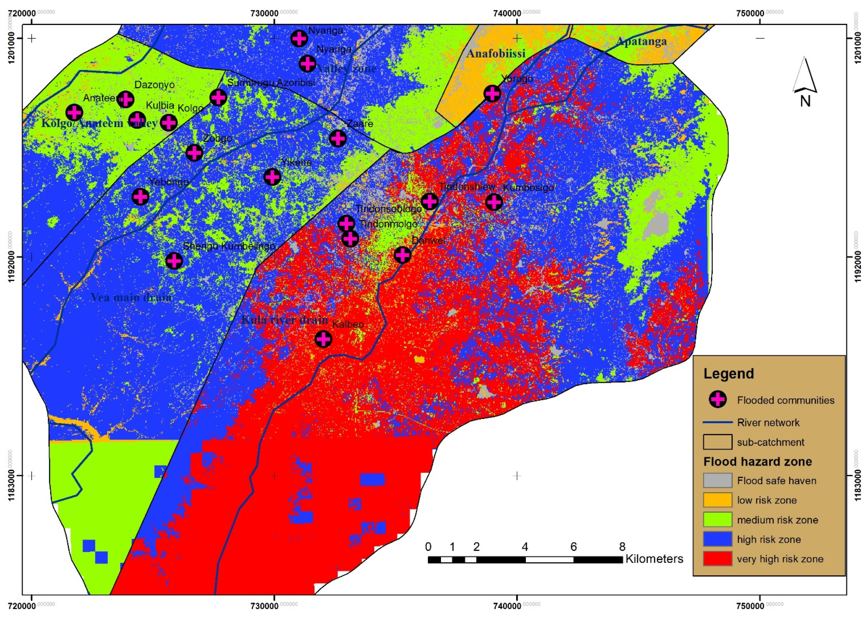
In addition to statistical validation procedure, the present study also relied on local expert knowledge and four-year historical records of flood events in the Vea study area where significant historical data is available. In this study area, 19 communities showed in Table 11 are generally known by local disaster managers, agriculture development officers and local people as highly prone to flood hazards. Consecutive flood events have been recorded in these communities since 2007 when local disaster managers started to systematically record flood events. In the qualitative validation process, these communities were plotted and then overlaid on the FHI map as shown in Figure 9.

The results (Figure 9) show that, of the communities listed as “flood prone” in Table 11, only 21% fall in the medium flood hazard intensity zone. The remaining 79% were all correctly classified by the flood modeling procedure used in this study as high flood prone communities. Of the communities that are classified as flood prone, 37% fall in the very high intensity whilst 42% fall in the high intensity zones. This suggests that the developed flood hazard index reasonably predicts areas likely to be flooded. It is interesting to note the result from the qualitative validation closely approximates the results achieved from the empirical validation process. In the Vea study area, the confusion matrix recorded a mapping accuracy of 77% and this is quite close to the 79% achieved with the qualitative validation with historical flood events.

Table 11. List of flood prone communities as listed by local agricultural authority. Source: District MoFA office, Bolgatanga.

Stretch of Valley	Communities	Operational Area	AEA Name
Kula River	Tindonshiew, Kumbosigo, Danwei, Tindonomolgo, Tindongsobiligo and Kalbeo	Zuarungu, Bolga Central and Kalbeo	Lambert, Maxwel and Iddrisu
Vea Main Drain	Nyariga, Yorogo, Zaare, Yikene, Sumbrungu Azoribisi, Zobgo, Sherigu Kumbelingo, Yebongo, Kulbia	Nyanga, Zaare/Yorogo, Sumbrungu East	Adongo Victoria, Thomas Anobiga, John Asigre and Hamza Akurubila
Kolgo/Anatem Valley	Kolgo, Dazongo, Anateem, Kulbia	Sumbrungu East and Sumbrungu West	Thomas Anobiga and John Asigre

Table 11. List of flood prone communities as listed by local agricultural authority. Source: District MoFA office, Bolgatanga.

Stretch of Valley	Communities	Operational Area	AEA Name
Kula River	Tindonshiew, Kumbosigo, Danwei, Tindonomolgo, Tindongsobiligo and Kalbeo	Zuarungu, Bolga Central and Kalbeo	Lambert, Maxwel and Iddrisu
Vea Main Drain	Nyariga, Yorogo, Zaare, Yikene, Sumbrungu Azoribisi, Zobgo, Sherigu Kumbelingo, Yebongo, Kulbia	Nyanga, Zaare/Yorogo, Sumbrungu East	Adongo Victoria, Thomas Anobiga, John Asigre and Hamza Akurubila
Kolgo/Anatem Valley	Kolgo, Dazongo, Anateem, Kulbia	Sumbrungu East and Sumbrungu West	Thomas Anobiga and John Asigre

Figure 9. Qualitative validation of FHI with local expert knowledge.

Figure 9. Qualitative validation of FHI with local expert knowledge.

4.6. Determining Flood Safe Havens

The 30 m spatial resolution of the final flood hazard map could be one ingredient to allow for accurate determination of areas normally safe from floods at the community level. Such areas are critical in periods of severe hazard occurrence. They are needed for evacuation plans, temporal shelters and provision of general relief efforts. However, accurate derivation of evacuation plans requires access routes to and from the flood zones [9], which was not investigated in this study.

The results obtained in this study can contribute to the development of community-based sustainable flood risk management plans that can ensure prevention, protection and preparedness for flood events. For example, effective community based education could help community members to identify agricultural areas on the map that fall within the high flood hazard zones and to avoid cultivating such areas during certain periods of the year. This will translate into a reduction in the socio-economic and environmental related losses that are mostly associated with the occurrence of floods and enhance efforts at achieving sustainable development in West Africa.

In Figure 10 for example, all the areas marked in green shades and classified as very low flood intensity zones could be considered as flood safe havens. In combination with field inspections with local people, these flood safe havens can be verified and marked as flood safe havens for the purpose of effective emergency management. Additionally, policy makers and development planners can, through an assessment of the flood hazard zones, develop appropriate policies and rules that will limit development in flood hot spots and consequently reduce the effects of flooding on the livelihoods of rural small holder farmers in the study watersheds.

Figure 10. Flood safe havens in Vea study area.

Figure 10. Flood safe havens in Vea study area.

5. Conclusions

The study has applied flood modeling approaches to demonstrate the feasibility of flood modeling in data scarce environments and limited resources. This study has drawn on the strengths of a simple hydrological model and statistical methods integrated in GIS to develop a Flood Hazard Index to an acceptable accuracy level. The flood hazard index shows that almost half of the study areas in Ghana and Benin falls into the “very high and high flood intensity zones” whilst more than half of the study area in Burkina Faso fall in high intensity flood zones.

The study also introduced an innovative flood modeling validation procedure using statistical and PGIS principles to evaluate the robustness of the methods used. Using the remote sensing technique of a confusion matrix, the overall accuracy of the flood hazard index was estimated at 77.62% in the Vea study area and 81.41% in the Dano study area.

The study also conducted qualitative validation of the results obtained for the Ghana site with local expert knowledge and found that the flood modeling methods accurately classified 79% of communities deemed to be highly susceptible to flood hazard and classified the remaining 21% into medium risk zone. The close similarity in the accuracy levels of the Vea flood Hazard index between the statistical-PGIS validation and qualitative assessment showed the robustness of the methods employed in mapping community flood hotspots.

Integration of the two approaches (hydrological and statistical) and combined with GIS and remote sensing techniques have shown the potential for diverse applications of the Flood Hazard Index. With this approach, flood risk of various land uses can be determined with a higher spatial resolution of 30 m. Such a high mapping scale could allow for accurate estimation of most flood risk elements and identification of flood safe havens.

However, although this approach has yielded an acceptable accurate Flood Hazard Index, it must be pointed out that under increased flood intensity occasioned by climate change, areas originally classified as flood safe havens under this model could offer protection, albeit only within the limits of the model inputs. For instance, an increase in rainfall intensity far beyond the anomalous (extreme) rainfall values used in this study could lead to the reclassification of these safe havens into another flood hazard intensity zone. This study also used a hydrological model which relied on globally available runoff coefficients to estimate the peak runoff values. These coefficients may not necessarily be exactly the same as those determined from field measurements in the study areas. In addition, the study did not investigate the contribution of flood inundation statistics such as flood depth, velocity, and progression as well as physical infrastructure which could also influence the intensity level of flooding. Again, lack of adequate data especially high resolution remote sensing imagery which necessitated the merging of courser resolution imagery for limited portions of the Dassari and Vea study areas should be taken into account in interpreting the results of the affected areas.

Flood risk is projected to increase with increasing exposure of populations and therefore effective flood management must include changes in the landscape that impacts the response to floods, locations of people and elements at risk [13]. Using this community level flood hazard map could contribute to effective disaster management operations as recommended by Kundzewics et al. [13] including prevention. For instance, in combination with high resolution satellite imagery, the FHI could help in rapid post-disaster assessments to estimate the economic impacts of flood disasters. This could be done by overlaying the maps of critical infrastructure in addition to detail land use maps.

Availability of “non-structural measures such as flood risk maps help in reducing flood risk in the area with relatively little investment” ([78], p. 5). In addition, the output from this approach will be very useful in the retrieval of socio-ecological indicators such as those identified in Asare-Kyei et al. [30] crucial for the assessment of risk and vulnerability in a coupled socio-ecological system in subsequent studies. The result of this study can be used by local disaster managers in Disaster Risk Reduction (DRR) and Health Emergency Preparedness and Response Programmes (HEPRP) and serve, among other things, “to build safer” public infrastructure, improve mass movement of “casualties during emergencies” ([20], p. 7) and help build more climate resilient rural communities.