
Runoff Response to Climate Warming and Forest Disturbance in a Mid-Mountain Basin


Abstract
:
1. Introduction
2. Materials and Methods
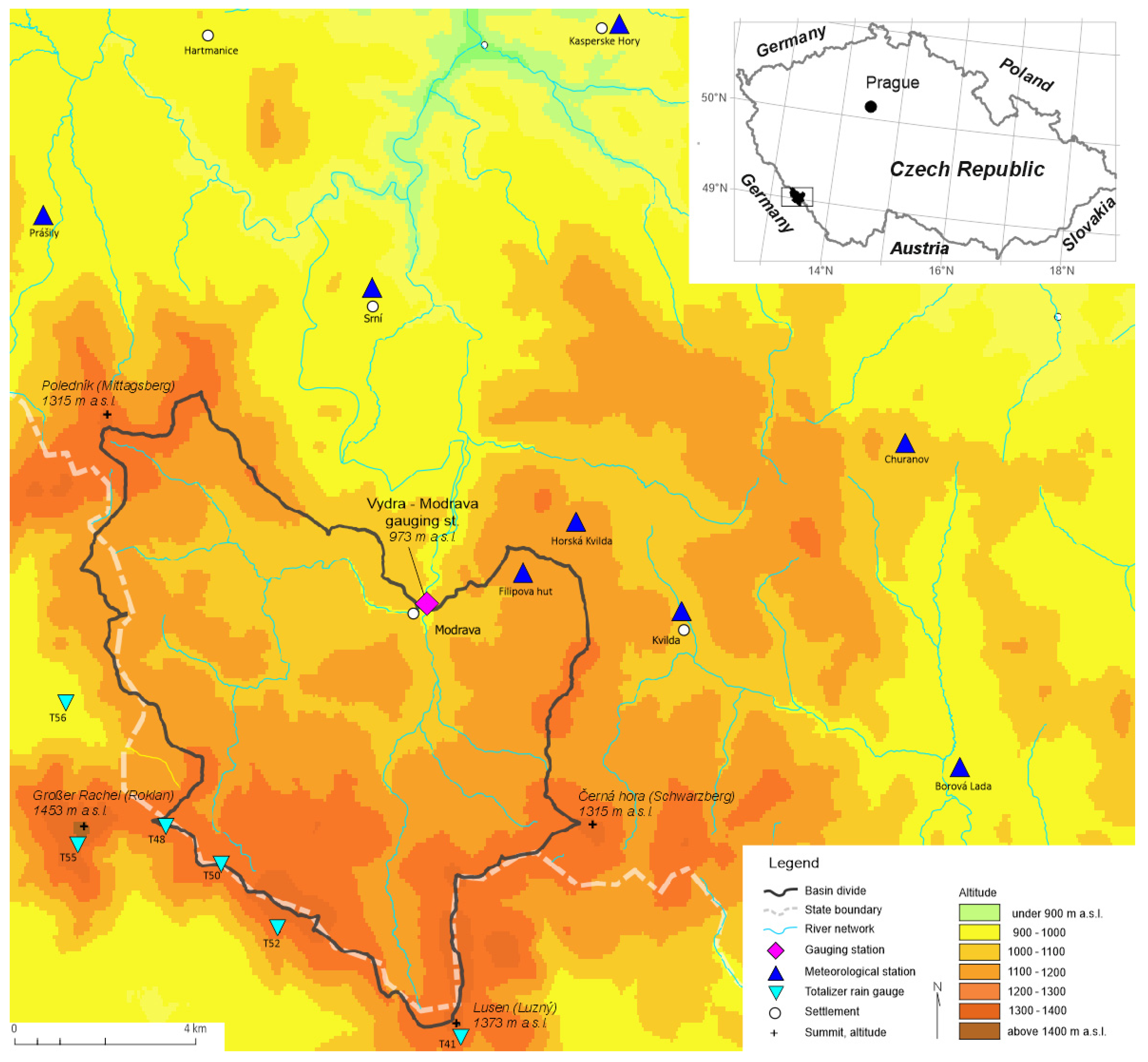
2.1. Study Area


| Basin/Unit | A [km2] | D [km km−2] | Hmean [m] | Hmin [m] | Hmax [m] | Smean [°] | Smax [°] | T [°C] | P [mm] | Q [mm] | C [–] |
|---|---|---|---|---|---|---|---|---|---|---|---|
| Upper Vydra | 89.7 | 2.3 | 1112 | 935 | 1373 | 7 | 55 | 3.6 | 1378 | 1175 | 0.85 |
2.2. Data Sources
2.3. Applied Methods
3. Results
3.1. Variability of Climatic Conditions

3.2. Homogeneity and Change Points in Time Series
| Category | Variable [unit] | Buishand’s Test | Petitt’s Test | ||||||||||
| p-value | Test Result | Date of Change | Risk of H0 Rejection | mean1 | mean2 | p-value | Test Result | Date of Change | Risk of H0 Rejection | mean1 | mean2 | ||
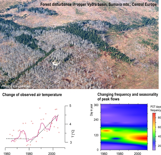
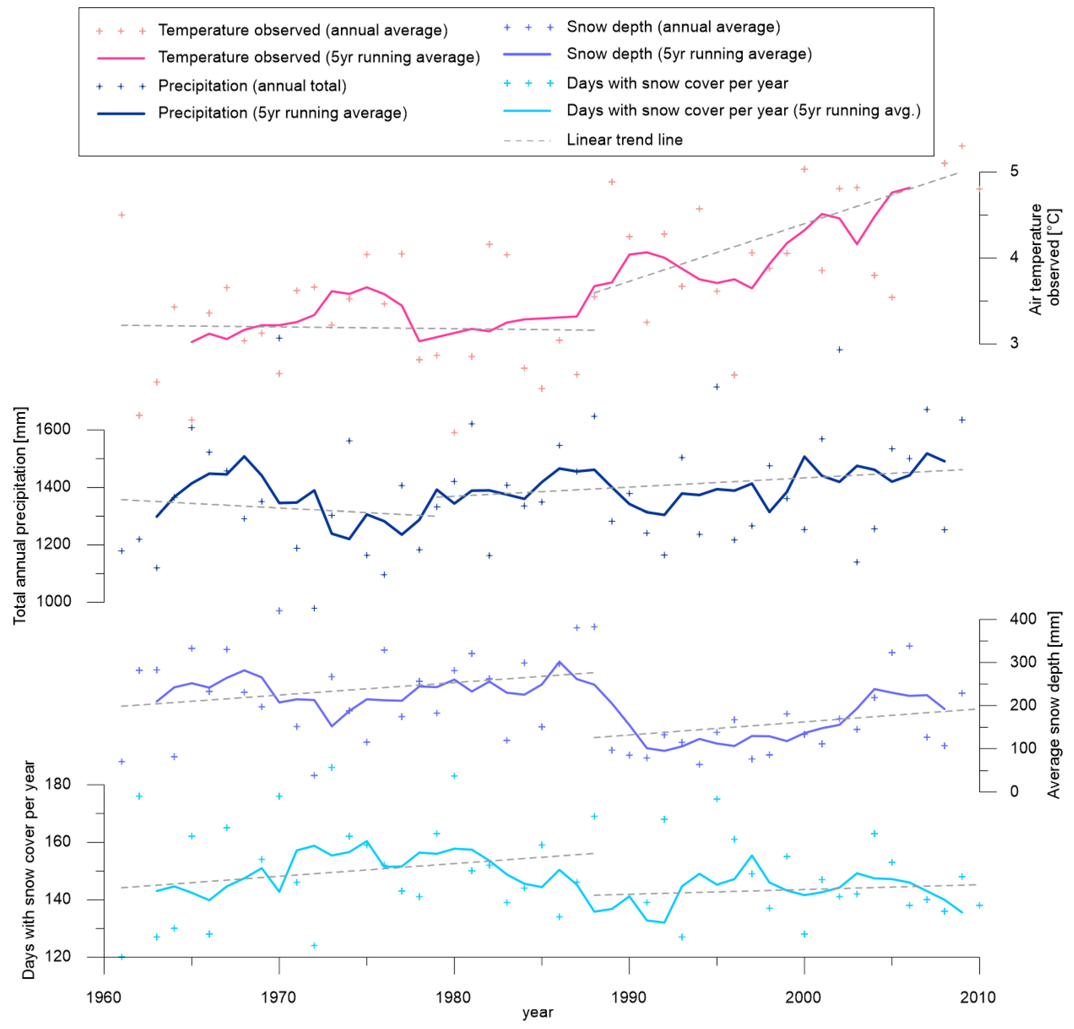
| Driving Forces | Air temperature [°C] | 0.0001 | Ha | 1988 | 0.01% | 3.19 | 4.134 | 0.0001 | Ha | 1988 | 0.01% | 3.19 | 4.13 |
| Precipitation [mm] | 0.714 | H0 | 1974 | 71.4% | 0.583 | H0 | 1979 | 58.3% | |||||
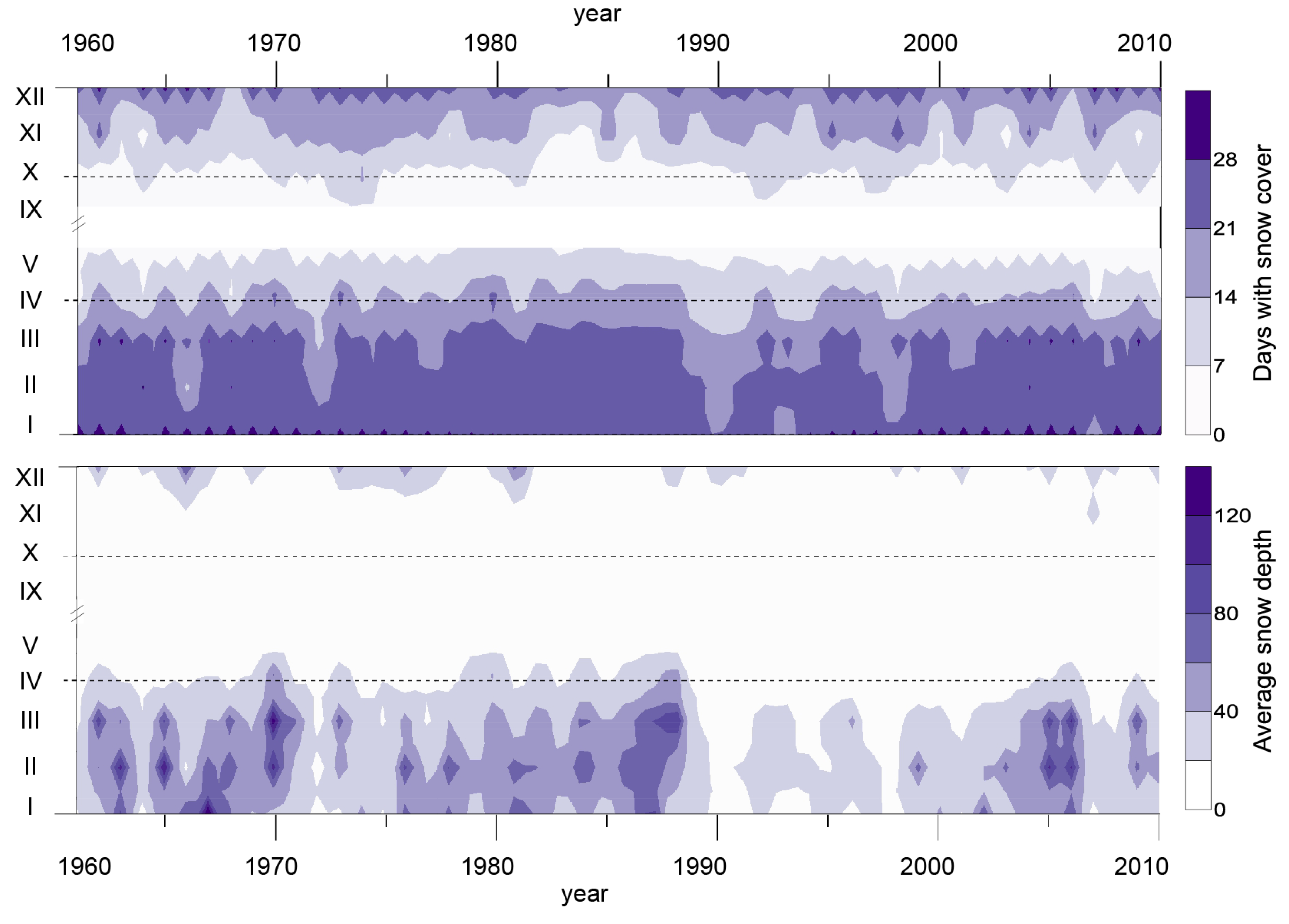
| Days with snow cover | 0.420 | H0 | 1988 | 42.0% | 0.267 | H0 | 1988 | 26.7% | |||||
| Mean snow cover depth [cm] | 0.005 | Ha | 1988 | 0.5% | 235.502 | 146.505 | 0.004 | Ha | 1988 | 0.4% | 235.51 | 146.52 | |
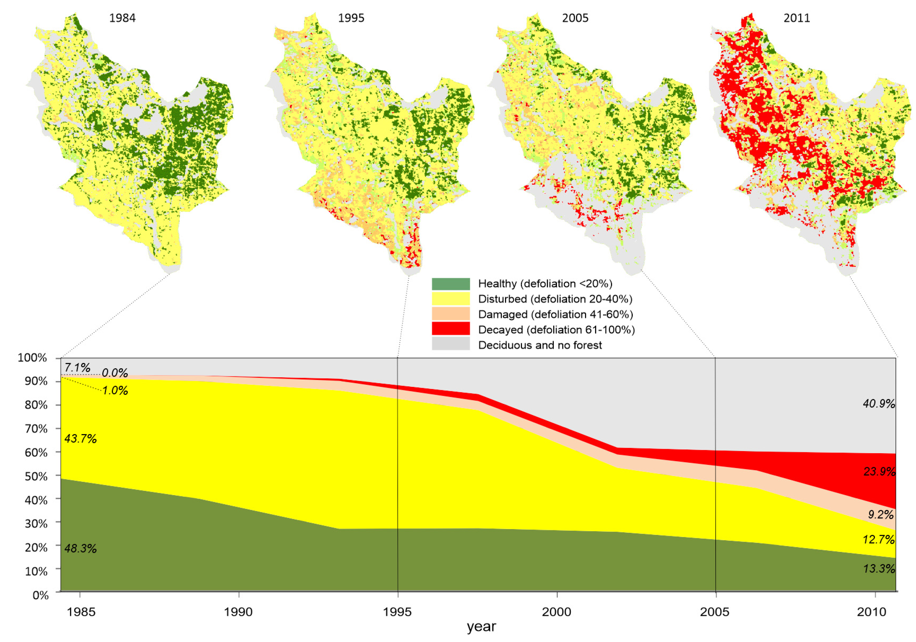
| Share of damaged and decayed forest area [%] | 0.0001 | Ha | 1993 | 0.01% | 2.7 | 19.2 | 0.001 | Ha | 1993 | 0.1% | 3 | 19 | |
| Runoff Balance | Qa [m3·s−1] | 0.152 | H0 | 1965 | 15.2% | 0.161 | H0 | 1965 | 16.1% | ||||
| Qmedian [m3·s−1] | 0.38 | H0 | 1964 | 38.0% | 0.202 | H0 | 1964 | 20.2% | |||||
| Direct flow [m3·s−1] | 0.0001 | Ha | 1988 | 0.01% | 0.261 | 0.175 | 0.0001 | Ha | 1988 | 0.01% | 0.26 | 0.17 | |
| Baseflow [m3·s−1] | 0.379 | H0 | 1964 | 37.9% | 0.614 | H0 | 1964 | 61.4% | |||||
| Baseflow index (BFI) [–] | 0.0001 | Ha | 1990 | 0.01% | 0.88 | 0.917 | 0.0001 | Ha | 1990 | 0.01% | 0.88 | 0.92 | |
| Runoff Variability | Q30d [m3·s−1] | 0.202 | H0 | 1985 | 20.2% | 0.205 | H0 | 1998 | 20.5% | ||||
| Q330d [m3·s−1] | 0.064 | H0 | 1964 | 6.4% | 0.134 | H0 | 1964 | 13.4% | |||||
| Q355d [m3·s−1] | 0.055 | H0 | 1964 | 5.5% | 0.134 | H0 | 1964 | 13.4% | |||||
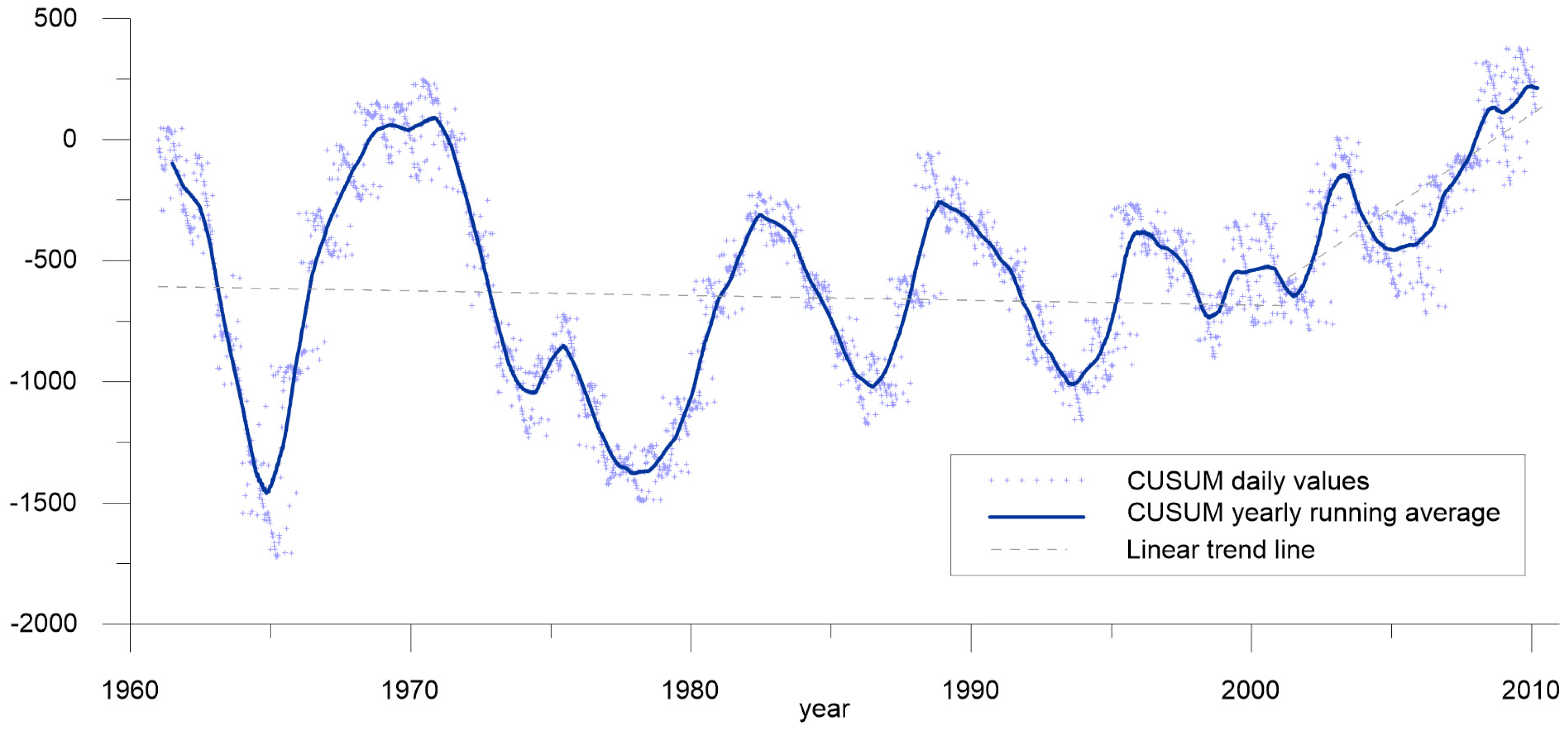
| Qd CUSUM [–] | 0.027 | Ha | 2001 | 2.7% | −235,900 | −45,909 | 0.022 | Ha | 2001 | 2.2% | −235,900 | −45,909 | |
| SD [–] | 0.016 | Ha | 1985 | 1.6% | 2.887 | 3.739 | 0.025 | Ha | 1985 | 2.5% | 2.88 | 3.74 | |
| Category | Variable [unit] | Buishand’s Test | Petitt’s Test | ||||||||||
| p-value | Test Result | Date of Change | Risk of H0 Rejection | p-value | Test Result | p-value | Test Result | p-value | Test Result | mean1 | mean2 | ||
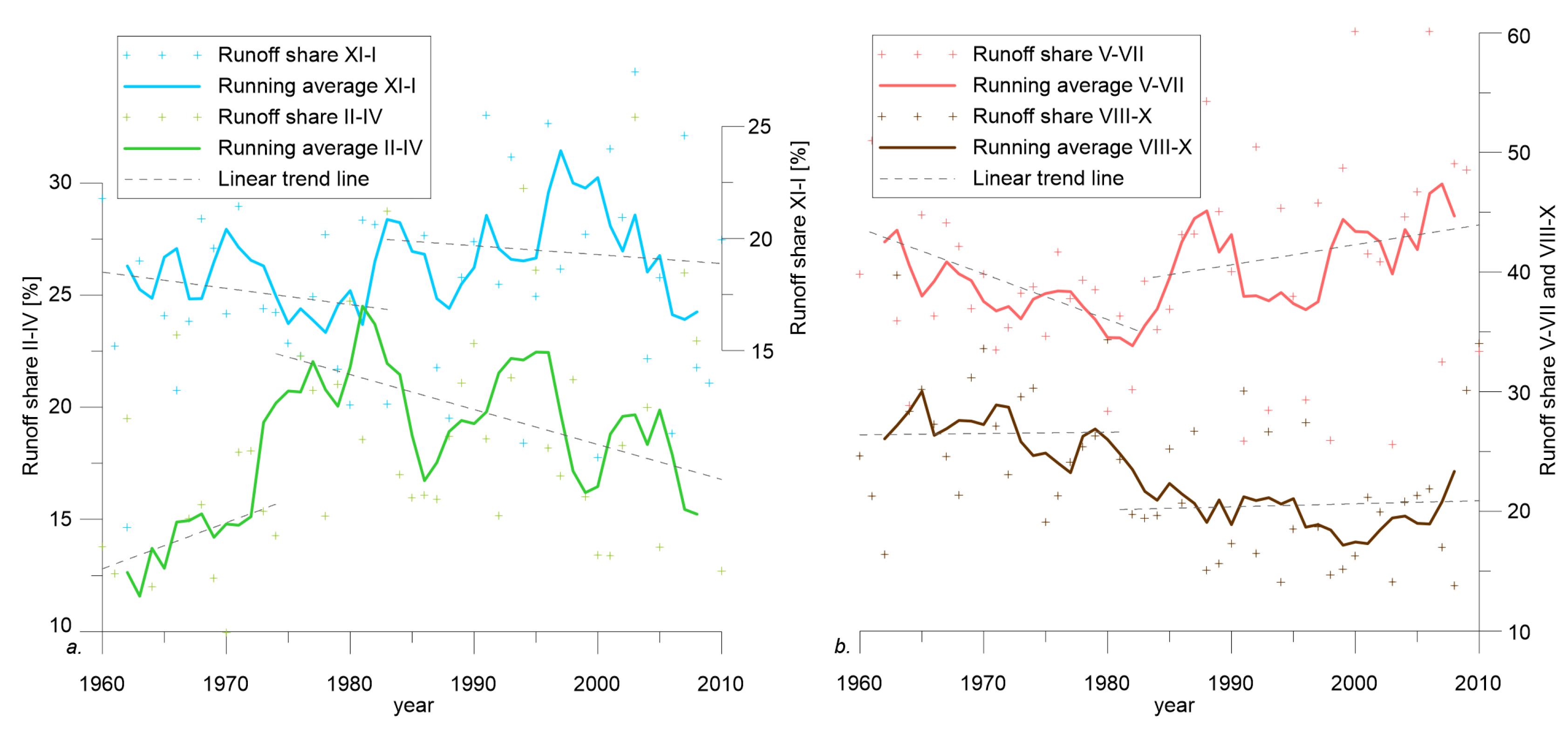
| Runoff Seasonality | Spring share (II-IV) [–] | 0.03 | Ha | 1974 | 3.0% | 0.142 | 0.199 | 0.016 | Ha | 1974 | 1.6% | 0.14 | 0.19 |
| Summer share (V-VII) [–] | 0.594 | H0 | 1998 | 59.4% | 0.513 | H0 | 1985 | 51.3% | |||||
| Fall share (VIII-X) [–] | 0.002 | Ha | 1981 | 0.2% | 0.265 | 0.205 | 0.001 | Ha | 1981 | 0.1% | 0.27 | 0.21 | |
| Winter share (XI-I) [–] | 0.693 | H0 | 1983 | 69.3% | 0.655 | H0 | 1983 | 65.5% | |||||
| Peak Flows and Low Flows | POT events [–] | 0.007 | Ha | 1994 | 0.7% | 3.765 | 6.063 | 0.011 | Ha | 1991 | 1.1% | 3.71 | 5.79 |
| POT days [–] | 0.125 | H0 | 1985 | 12.5% | 0.08 | H0 | 1985 | 8.0% | |||||
| POT event duration [–] | 0.277 | H0 | 1985 | 27.7% | 0.492 | H0 | 1985 | 49.2% | |||||
| 1-2day long POT event [–] | 0.003 | Ha | 1994 | 0.3% | 2.73 | 4.16 | 0.002 | Ha | 1994 | 0.2% | 2.73 | 4.16 | |
| LOF events [–] | 0.128 | H0 | 1977 | 12.8% | 0.069 | H0 | 1977 | 6.9% | |||||
| LOF days [–] | 0.0001 | Ha | 1964 | 0.01% | 103.6 | 21.571 | 0.049 | H0 | 1964 | 4.9% | 103.60 | 21.57 | |
| LOF event duration [days] | 0.251 | H0 | 2004 | 25.1% | 0.294 | H0 | 2001 | 29.4% | |||||
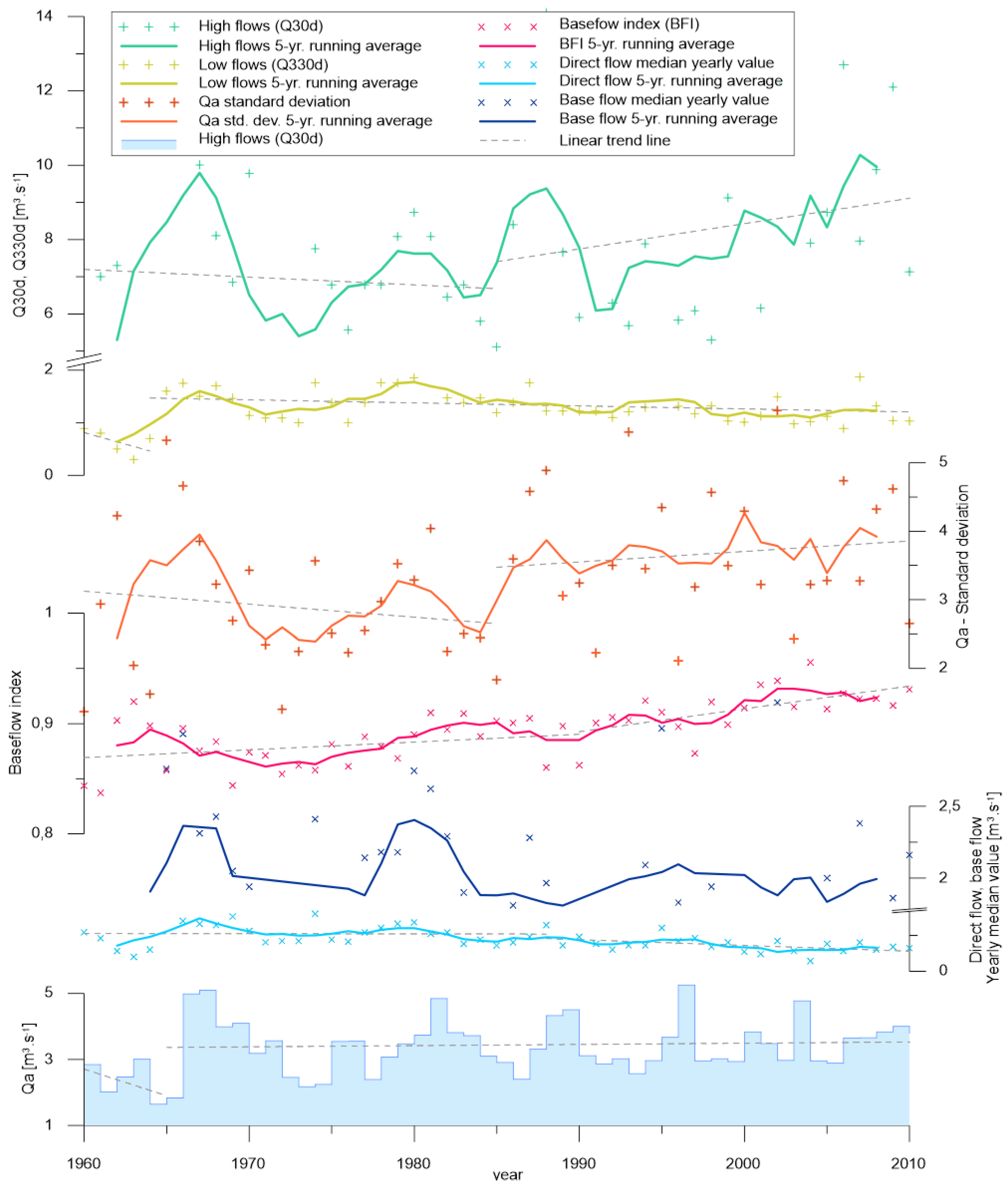
3.3. Changes in Runoff Balance and Variability

3.4. Changes of Seasonal Runoff Distribution
| Parameter | Station | XI-I | II-IV | VI-VIII | IX-XI | I | II | III | IV | V | VI | VII | VIII | IX | X | XI | XII |
|---|---|---|---|---|---|---|---|---|---|---|---|---|---|---|---|---|---|
| P | Churanov | ||||||||||||||||
| Kvilda | |||||||||||||||||
| Filipova Hut | |||||||||||||||||
| Q | Modrava | ||||||||||||||||
| p ≤ 0.01 | |||||||||||||||||
| p ≤ 0.05 | |||||||||||||||||
| Non-significant trend | |||||||||||||||||
| No trend | |||||||||||||||||

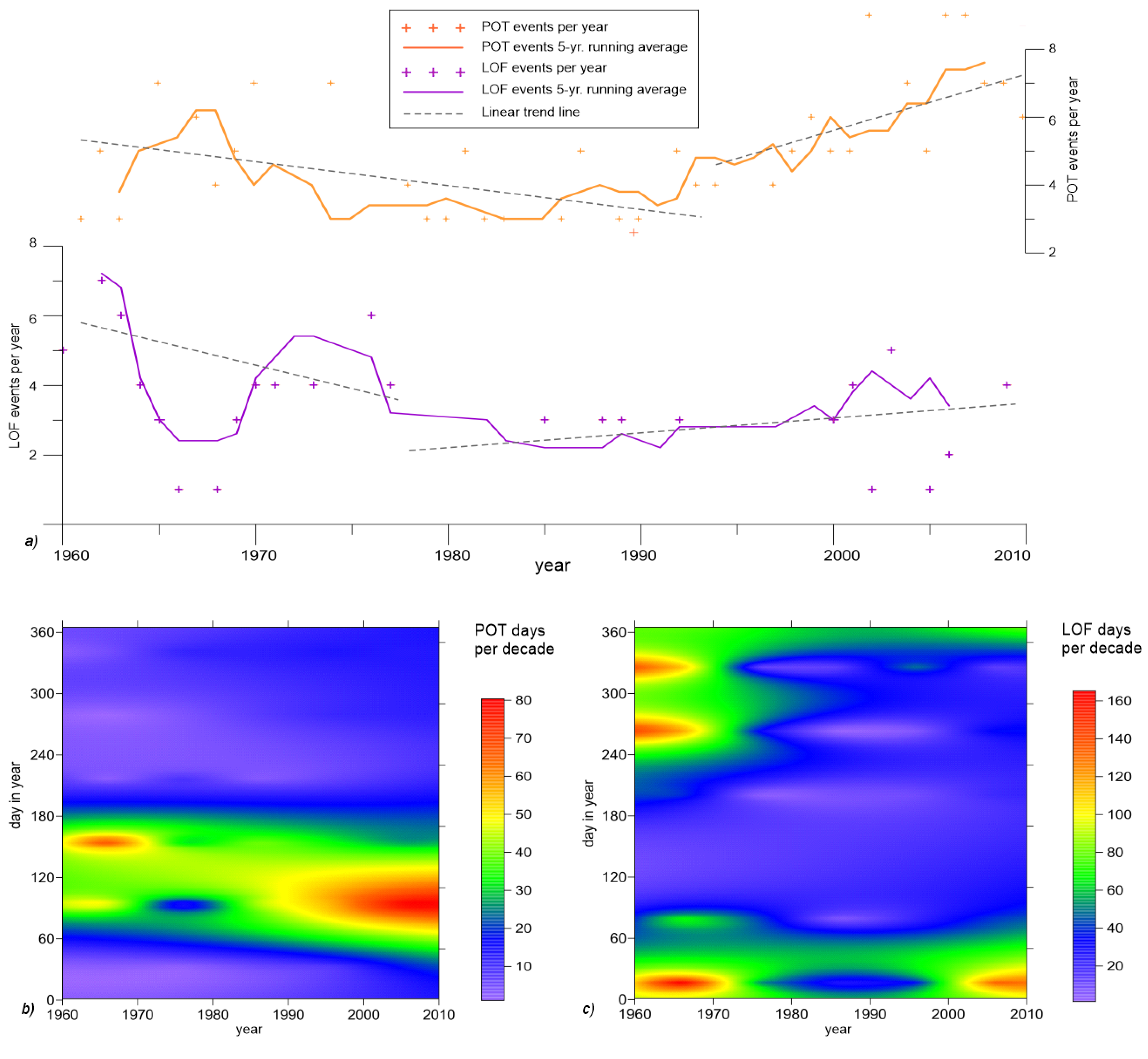
3.5. Variability and Seasonality of Peak Flows and Low Flows
4. Discussion
5. Conclusions
Supplementary Materials
Acknowledgments
Author Contributions
Conflicts of Interest
References
- Burn, D.H.; Elnur, M.A.H. Detection of hydrologic trends and variability. J. Hydrol. 2002, 255, 107–122. [Google Scholar] [CrossRef]
- Intergovernmental Panel on Climate Change (IPCC). Summary for Policymakers. In Climate Change 2014, Mitigation of Climate Change; Cambridge University Press: Cambridge, UK; New York, NY, USA, 2013; pp. 19–23. [Google Scholar]
- Kliment, Z.; Matouskova, M. Runoff changes in the Sumava mountains (Black Forest) and the foothill regions: Extent of influence by human impact and climate change. Water Resour. Manag. 2009, 23, 1813–1834. [Google Scholar] [CrossRef]
- Wei, X.; Liu, W.; Zhou, P. Quantifying the relative contributions of forest change and climatic variability to hydrology in large watersheds: A critical review of research methods. Water 2013, 5, 728–746. [Google Scholar] [CrossRef]
- Al-Faraj, F.A.; Scholz, M.; Tigkas, D. Sensitivity of surface runoff to drought and climate change: Application for shared river basins. Water 2014, 6, 3033–3048. [Google Scholar] [CrossRef]
- Dam, J.C. Impacts of Climate Change and Variability on Hydrological Regimes; Cambridge Univeristy Press: Cambridge, UK, 1999. [Google Scholar]
- Dvorak, V.; Hladny, J.; Kasparek, L. Climate change hydrology and water resources impact and adaptation for selected river basins in the Czech republic. Clim. Chang. 1997, 36, 93–106. [Google Scholar] [CrossRef]
- Li, F.; Zhang, G.; Xu, Y. Separating the impacts of climate variation and human activities on runoff in the Songhua River basin, northeast China. Water 2014, 6, 3320–3338. [Google Scholar] [CrossRef]
- Blöschl, G.; Ardoin-Bardin, S.; Bonell, M.; Dorninger, M.; Goodrich, D.; Gutknecht, D.; Matamoros, D.; Merz, B.; Shand, P.; Szolgay, J. At what scales do climate variability and land cover change impact on flooding and low flows? Hydrol. Process. 2007, 21, 1241–1247. [Google Scholar] [CrossRef]
- Tomer, M.D.; Schilling, K.E. A simple approach to distinguish land-use and climate-change effects on watershed hydrology. J. Hydrol. 2009, 376, 24–33. [Google Scholar] [CrossRef]
- Zheng, H.; Zhang, L.; Zhu, R.; Liu, C.; Sato, Y.; Fukushima, Y. Responses of streamflow to climate and land surface change in the headwaters of the yellow river basin. Water Resour. Res. 2009, 45, W00A19. [Google Scholar] [CrossRef]
- Palamuleni, L.; Ndomba, P.; Annegarn, H. Evaluating land cover change and its impact on hydrological regime in upper Shire River catchment, Malawi. Reg. Environ. Chang. 2011, 11, 845–855. [Google Scholar] [CrossRef]
- Ma, X.; Xu, J.; van Noordwijk, M. Sensitivity of streamflow from a himalayan catchment to plausible changes in land cover and climate. Hydrol. Process. 2010, 24, 1379–1390. [Google Scholar] [CrossRef]
- Dung, B.X.; Gomi, T.; Miyata, S.; Sidle, R.C.; Kosugi, K.; Onda, Y. Runoff responses to forest thinning at plot and catchment scales in a headwater catchment draining japanese cypress forest. Journal of Hydrology 2012, 444, 51–62. [Google Scholar] [CrossRef]
- Bosch, J.M.; Hewlett, J.D. A review of catchment experiments to determine the effect of vegetation changes on water yield and evapotranspiration. J. Hydrol. 1982, 55, 3–23. [Google Scholar] [CrossRef]
- Ide, J.; Finer, L.; Lauren, A.; Piirainen, S.; Launiainen, S. Effects of clear-cutting on annual and seasonal runoff from a boreal forest catchment in eastern Finland. For. Ecol. Manag. 2013, 304, 482–491. [Google Scholar] [CrossRef]
- Buttle, J.M.; Metcalfe, R.A. Boreal forest disturbance and streamflow response, northeastern Ontario. Can. J. Fish. Aquat. Sci. 2000, 57, 5–18. [Google Scholar] [CrossRef]
- Beudert, B.; Klöcking, B.; Marcq, B.; Niederberger, J.; Puhlmann, H.; Schwarze, R.; Wilpert, K.-H.V. Forest Hydrology-Results of Research in Germany and Russia; ihp.hwrp: Koblenz, Germany, 2007; p. 131. [Google Scholar]
- Pomeroy, J.; Fang, X.; Ellis, C. Sensitivity of snowmelt hydrology in Marmot creek, Alberta, to forest cover disturbance. Hydrol. Process. 2012, 26, 1891–1904. [Google Scholar] [CrossRef]
- Troendle, C.A.; Reuss, J.O. Effect of clearcutting on snow accumulation and water outflow at Fraser, Colorado. Hydrol. Earth Syst. Sci. 1997, 1, 325–332. [Google Scholar] [CrossRef]
- Kuraś, P.K.; Alila, Y.; Weiler, M. Forest harvesting effects on the magnitude and frequency of peak flows can increase with return period. Water Resour. Res. 2012, 48, W01544. [Google Scholar] [CrossRef]
- Robinson, M.; Cognard-Plancq, A.-L.; Cosandey, C.; David, J.; Durand, P.; Führer, H.-W.; Hall, R.; Hendriques, M.; Marc, V.; McCarthy, R. Studies of the impact of forests on peak flows and baseflows: A European perspective. For. Ecol. Manag. 2003, 186, 85–97. [Google Scholar] [CrossRef]
- Brown, A.E.; Western, A.W.; McMahon, T.A.; Zhang, L. Impact of forest cover changes on annual streamflow and flow duration curves. J. Hydrol. 2013, 483, 39–50. [Google Scholar] [CrossRef]
- Rex, J.; Dubé, S.; Foord, V. Mountain pine beetles, salvage logging, and hydrologic change: Predicting wet ground areas. Water 2013, 5, 443–461. [Google Scholar] [CrossRef]
- Zhang, M.; Wei, X. The effects of cumulative forest disturbance on streamflow in a large watershed in the central interior of British Columbia, Canada. Hydrol. Earth Syst. Sci. 2012, 16, 2021–2034. [Google Scholar] [CrossRef] [Green Version]
- Zemek, F.; Herman, M. Bark beetle—A stress factor of spruce forests in the Bohemian Forest. Ekol. Bratisl. 2001, 20, 95–107. [Google Scholar]
- Stednick, J.D. Monitoring the effects of timber harvest on annual water yield. J. Hydrol. 1996, 176, 79–95. [Google Scholar] [CrossRef]
- Hais, M.; Jonášová, M.; Langhammer, J.; Kučera, T. Comparison of two types of forest disturbance using multitemporal landsat tm/etm+ imagery and field vegetation data. Remote Sens. Environ. 2009, 113, 835–845. [Google Scholar] [CrossRef]
- Birsan, M.-V.; Molnar, P.; Burlando, P.; Pfaundler, M. Streamflow trends in switzerland. J. Hydrol. 2005, 314, 312–329. [Google Scholar] [CrossRef]
- Vacek, S.; Podrazsky, V. Forest ecosystems of the Sumava mts. and their management. J. For. Sci. 2003, 49, 291–301. [Google Scholar]
- Českého Hydrometeorologického Ústavu (ČHMÚ). Climatic Atlas of Czechia.; ČHMÚ: Prague, Czech Republic, 2007; p. 256. [Google Scholar]
- Čurda, J.; Janský, B.; Kocum, J. The effects of physical-geographic factors on flood episodes extremity in the Vydra river basin. Geografie 2011, 116, 335–353. [Google Scholar]
- Křenová, Z.; Hruška, J. Proper zonation—An essential tool for the future conservation of the Sumava national park. Eur. J. Environ. Sci. 2012, 2, 62–72. [Google Scholar]
- Czech Hydrometeorological Institute (CHMI). Precipitation and Runoff Database; CHMI: Prague, Czech Republic, 2013.
- Czech Hydrometeorological Institute (CHMI). Snow Cover Database; CHMI: Prague, Czech Republic, 2015.
- Český Úřad Zeměměřický a Katastrální (CUZK). 4G Digital Elevation Model; CUZK: Prague, Czech Republic, 2013. [Google Scholar]
- Brázdil, K.; Bělka, L.; Dušánek, P.; Fiala, R.; Gamrát, J.; Kafka, O.; Peichl, J.; Šíma, J. Technical Report to the 4G Digital Elevation Model; CUZK: Prague, Czech Republic, 2012. [Google Scholar]
- DIgitální BÁze VOdohospodářských Dat (DIBAVOD). Available online: http://www.dibavod.cz/ (accessed on 5 October 2014).
- Langhammer, J.; Hartvich, F.; Mattas, D.; Rödlová, S.; Zbořil, A. The variability of surface water quality indicators in relation to watercourse typology, Czech Republic. Environ. Monit. Assess. 2012, 184, 3983–3999. [Google Scholar] [CrossRef] [PubMed]
- UHUL. Maps of the Health Condition of Czech Republic Forests Based on Satellite Images. Available online: http://geoportal.uhul.cz/mapy/mapyzsl.html (accessed on 15 November 2014).
- Kendall, M.G. Rank Correlation Methods; Griffin: London, UK, 1948. [Google Scholar]
- Hamed, K.H. Trend detection in hydrologic data: The mann-kendall trend test under the scaling hypothesis. J. Hydrol. 2008, 349, 350–363. [Google Scholar] [CrossRef]
- Eckhardt, K. How to construct recursive digital filters for baseflow separation. Hydrol. Process. 2005, 19, 507–515. [Google Scholar] [CrossRef]
- Nathan, R.; McMahon, T. Evaluation of automated techniques for base flow and recession analyses. Water Resour. Res. 1990, 26, 1465–1473. [Google Scholar] [CrossRef]
- Lim, K.J.; Engel, B.A.; Tang, Z.; Choi, J.; Kim, K.S.; Muthukrishnan, S.; Tripathy, D. Automated Web GIS Based Hydrograph Analysis Tool, WHAT1; Wiley/John Wiley & Sons Inc: Hoboken, NJ, USA, 2005. [Google Scholar]
- Chen, X.C.; Steinhaeuser, K.; Boriah, S.; Chatterjee, S.; Kumar, V. Contextual Time Series Change Detection. In Proceedings of the 13th SIAM International Conference on Data Mining, Austin, TX, USA, 2–4 May 2013; pp. 503–511.
- Jessop, B.M.; Harvie, C.J. A CUSUM Analysis of Discharge Patterns by a Hydroelectric Dam and Discussion of Potential Effects on the Upstream Migration of American Eel Elvers; Government of Canada Publications: Dartmouth, NS, Canada, 2003.
- Buishand, T.A. Some methods for testing the homogeneity of rainfall records. J. Hydrol. 1982, 58, 11–27. [Google Scholar] [CrossRef]
- Machiwal, D.; Jha, M. Efficacy of Time Series Tests: A Critical Assessment. In Hydrologic time Series Analysis: Theory and Practice; Springer Netherlands: Dordrecht, The Netherlands, 2012; pp. 139–164. [Google Scholar]
- Taxak, A.K.; Murumkar, A.; Arya, D. Long term spatial and temporal rainfall trends and homogeneity analysis in Wainganga basin, central India. Weather. Clim. Extrem. 2014, 4, 50–61. [Google Scholar] [CrossRef]
- Costa, A.C.; Soares, A. Homogenization of climate data: Review and new perspectives using geostatistics. Math. Geosci. 2009, 41, 291–305. [Google Scholar] [CrossRef]
- Kang, H.M.; Yusof, F. Homogeneity tests on daily rainfall series. Int. J. Contemp. Math. Sciences 2012, 7, 9–22. [Google Scholar]
- Bässler, C. Klimawandel—Trend der Lufttemperatur im Inneren Bayerischen Wald (Böhmerwald). Silva. Gabreta. 2008, 14, 1–18. [Google Scholar]
- Lundberg, A.; Nakai, Y.; Thunehed, H.; Halldin, S. Snow accumulation in forests from ground and remote-sensing data. Hydrol. Process. 2004, 18, 1941–1955. [Google Scholar] [CrossRef]
- Schnorbus, M.; Werner, A.; Bennett, K. Quantifying the Water Resource Impacts of Mountain Pine Beetle and Associated Salvage Harvest Operations across a Range of Watershed Scales: Hydrologic Modeling of the Fraser River Basin; Pacific Forestry Centre: Victoria, BC, Canada, 2010; p. 423. [Google Scholar]
- Ogden, F.L.; Crouch, T.D.; Stallard, R.F.; Hall, J.S. Effect of land cover and use on dry season river runoff, runoff efficiency, and peak storm runoff in the seasonal tropics of central Panama. Water Resour. Res. 2013, 49, 8443–8462. [Google Scholar] [CrossRef]
- Redding, T.; Lapp, S.; Leach, J. Natural disturbance and post-disturbance management effects on selected watershed values. J. Ecosyst. Manag. 2012, 13, 1–14. [Google Scholar]
- Smerdon, B.D.; Redding, T.; Beckers, J. An overview of the effects of forest management on groundwater hydrology. J. Ecosyst. Manag. 2009, 10, 22–44. [Google Scholar]
- Bearup, L.A.; Maxwell, R.M.; Clow, D.W.; McCray, J.E. Hydrological effects of forest transpiration loss in bark beetle-impacted watersheds. Nat. Clim. Chang. 2014, 4, 481–486. [Google Scholar] [CrossRef]
- Jones, J.A. Hydrologic processes and peak discharge response to forest removal, regrowth, and roads in 10 small experimental basins, Western Cascades, Oregon. Water Resour. Res. 2000, 36, 2621–2642. [Google Scholar] [CrossRef]
- Waterloo, M.J.; Schellekens, J.; Bruijnzeel, L.A.; Rawaqa, T.T. Changes in catchment runoff after harvesting and burning of a Pinus Caribaea plantation in Viti Levu, Fiji. Ecol. Manag. 2007, 251, 31–44. [Google Scholar] [CrossRef]
- Krám, P.; Beudert, B.; Červenková, J.; Čech, J.; Váňa, M.; Fottová, D.; Dieffenbach-Fries, H. Daily streamwater runoff characteristics of the ICP IM catchments (CZ01, CZ02, DE01) in the Bohemian massif. Finn. Environ. 2008, 28, 39–46. [Google Scholar]
© 2015 by the authors; licensee MDPI, Basel, Switzerland. This article is an open access article distributed under the terms and conditions of the Creative Commons Attribution license (http://creativecommons.org/licenses/by/4.0/).
Share and Cite
Langhammer, J.; Su, Y.; Bernsteinová, J. Runoff Response to Climate Warming and Forest Disturbance in a Mid-Mountain Basin. Water 2015, 7, 3320-3342. https://doi.org/10.3390/w7073320
Langhammer J, Su Y, Bernsteinová J. Runoff Response to Climate Warming and Forest Disturbance in a Mid-Mountain Basin. Water. 2015; 7(7):3320-3342. https://doi.org/10.3390/w7073320
Chicago/Turabian StyleLanghammer, Jakub, Ye Su, and Jana Bernsteinová. 2015. "Runoff Response to Climate Warming and Forest Disturbance in a Mid-Mountain Basin" Water 7, no. 7: 3320-3342. https://doi.org/10.3390/w7073320