Spatio-Temporal Impacts of Biofuel Production and Climate Variability on Water Quantity and Quality in Upper Mississippi River Basin

Abstract

Impact of climate change on the water resources of the United States exposes the vulnerability of feedstock-specific mandated fuel targets to extreme weather conditions that could become more frequent and intensify in the future. Consequently, a sustainable biofuel policy should consider: (a) how climate change would alter both water supply and demand; and (b) in turn, how related changes in water availability will impact the production of biofuel crops; and (c) the environmental implications of large scale biofuel productions. Understanding the role of biofuels in the water cycle is the key to understanding many of the environmental impacts of biofuels. Therefore, the focus of this study is to model the rarely explored interactions between land use, climate change, water resources and the environment in future biofuel production systems. Results from this study will help explore the impacts of the US biofuel policy and climate change on water and agricultural resources. We used the Soil and Water Assessment Tool (SWAT) to analyze the water quantity and quality consequences of land use and land management related changes in cropping conditions (e.g., more use of marginal lands, greater residue harvest, increased yields), plus management practices due to biofuel crops to meet the Renewable Fuel Standard target on water quality and quantity.

1. Introduction

The United States is the largest consumer of crude oil in the world and is dependent on foreign sources for up to 60 percent of its consumption [1]. Moreover, fossil fuels contribute about 30 percent of all carbon-dioxide (CO₂) emissions in the US thereby raising concerns over global climate change [1]. As a result, renewable biofuels offer an excellent alternative energy source to petroleum-based fuels. In addition, they also have the potential to improve U.S. energy security, and mitigate climate change while enhancing rural economies. Biofuels (i.e., biomass derived fuels) are transportation fuels derived from biomass including grains, sugarcane, oil crops, cellulosic materials such as grasses, crop residue, and trees and other organic wastes [2]. Bioethanol and biodiesel are the two main types of biofuels. Although, biofuels account for only 2% of the global annual gasoline consumption of 1200 billion liters, their contribution to global energy supply is expected to increase rapidly in response to dwindling fossil fuel resources, increased demand, increasing cost of crude oil, concerns over greenhouse gasses (GHG), and new policies in place. The 2007 Energy Independence and Security Act (EISA) mandate a total annual production of 136 billion liters renewable fuels, including 79 billion liters of cellulosic biofuels, by 2022. The Renewable Fuel Standard (RFS) provides guidelines for the amount of blended biofuels (cellulosic, advanced, biomass-based diesel and conventional biofuels) production between 2008 and 2022, with a cap of 15 billion gallons annually for ethanol from corn grain while the rest (16 billion gallons) must be produced from cellulosic feedstock [1]. In the United States, biofuel production has historically focused on grain-based feedstock and is concentrated in the mid-western states [3]. However, current production of corn is not able to support the increasing demand for biofuel feedstock without threatening food security and raising food prices [4]. Therefore, lignocellulosic sources are also being considered including switchgrass, miscanthus, biomass sorghum, energycane, crop residues, hybrid poplar, willow, forest residues, and other forest products [5]. These feedstocks would serve as alternatives to corn and other traditional feedstocks to produce second-generation biofuel. Use of such feedstocks may reduce land competition due to higher biomass productivity and greater adaptability to different soil and climate conditions by using marginal lands [4,6]. However, scaling up the production of ligno-cellulosic biofuels will result in regional changes in land cover and cropping systems.

Since, bioenergy crop production is expected to expand rapidly to meet the U.S. government mandate for major increase in biofuel supply, it is important to optimize bioenergy crop selection, and evaluate the impact of large-scale bioenergy crop production systems on land use and sustainability, soil erosion, nutrient losses, and water resource. Moreover, the requirement of substantial amounts of water for biomass production exposes the vulnerability of feedstock-specific mandated fuel targets to extreme weather conditions that could become more frequent and intensify in the future as concluded by the Intergovernmental Panel on Climate Change (IPCC) in its 2007 report on climate change. More specifically, temperatures in the US has risen by 2 °C over the past 50 years and by the end of the century, the average U.S. temperature is expected to increase by approximately 4–5 °C under the higher emissions scenario and by approximately 2–3 °C under the lower emissions scenarios [7]. On a seasonal basis, most of the United States is projected to experience greater warming in summer than in winter, while Alaska experiences far more warming in winter than summer. In addition, precipitation across the United States has increased by an average of about 5–10 percent over the past 50 years [8]. As a result there will be significant impact on water resources through seasonal shifts in streamflow, changes in extreme high and low flow events, changes in groundwater recharge, changes in loadings and transport of sediments and nutrients due to changes in precipitation patterns and intensity, changes in frequency of occurrence of floods and drought, early melting of snow and ice, increasing evaporation and changes in soil moisture. Since, water that is needed to grow the biofuel crops is either available from natural precipitation and soil moisture or fed by irrigation from surface or groundwater resources, biofuel crops are vulnerable to droughts and to long-term climate-induced water stress. Therefore, climate variations will affect crop water use that in turn will affect the regional and local water balances. Furthermore, increase or decrease in the crop growth may result in an increase or decrease in sediment and nutrient in the water due to erosion and nutrient runoff. This will have implications for regional and local water quantity and quality affecting both ground and surface waters as runoff containing sediments, nitrogen and phosphorus can lead to over enrichment and excessive growth of algae in surface waters. Such enrichment can reduce water clarity, and decrease the oxygen content in the water, which in turn can damage aquatic life. One such example is the Northern Gulf of Mexico hypoxic zone which is currently the second largest in the western Atlantic Ocean [9]. On assessing the causes and consequences of the hypoxic conditions in the Northern Gulf of Mexico it has been found out that nitrogen (N) and phosphorus (P) loads discharged from the Mississippi River Basin (the major biofuel crop growing area) are the primary cause [10].

Although significant research has been accomplished on impacts of first generation biofuels related to land use [4,11], water consumption [12,13], water quality [14,15], environmental impacts of 2nd generation biofuels like switchgrass has been studied less. De La Torre Ugarte et al. [16] examined the effects of two cellulosic ethanol production expansion scenarios on agriculture, water demand, and water quality in the U.S. while studies by Secchi et al. [5] and Wu et al. [17] looked at water quality implications of switchgrass and corn. Their studies concluded that the switchgrass resulted in greater reduction of phosphorus and potassium runoff, however the nitrogen runoff was unchanged. Wu et al. [18,19] studied the impact of landuse change due to biofuel production in Midwestern watersheds. Ng et al. [20] modeled the water quality impacts of growing Miscanthus. Evans and Cohen [21] studied the implications of bioethanol production in Florida and Georgia and indicated that bioenergy production of corn, sugarcane, sweet sorghum, and southern pine will offset 17.5% of regional gasoline consumption on a gross energy basis, but much less on a net energy basis, and would require substantial input of nitrogen, water, and land. In addition, recent studies by Zhuang et al. [22] and VanLoocke et al. [23] compared the water efficiencies of first and second generation bioenergy crops.

Most of the previous and current research is useful for providing preliminary estimates of the environmental sustainability of conventional or cellulosic bioenergy production systems without considering climate change and variability such as that of Demissie et al. [24]. They studied the water quality impacts of biofuel production in the Upper Mississippi River basin but did not take climate variability into consideration. Nevertheless, Brown et al. [25], Dominguez-Faus et al. [12], and Tulbure et al. [26] are amongst the very few who have analyzed the impacts of a changing climate on production of bioenergy crops. However, they do not consider the alterations in the hydrologic cycle driven by a combination of biomass feedstock production and climate change and therefore the results have limited use in assessing environmental impact and sustainability of large scale bio feedstock production systems. Therefore, the overall scope of this paper is to examine how biofuels expansion strategies under a variable climate impacts the long term water availability and water quality. More specifically this paper will answer questions such as:

(1)

Where is water availability likely to be a limiting factor?

(2)

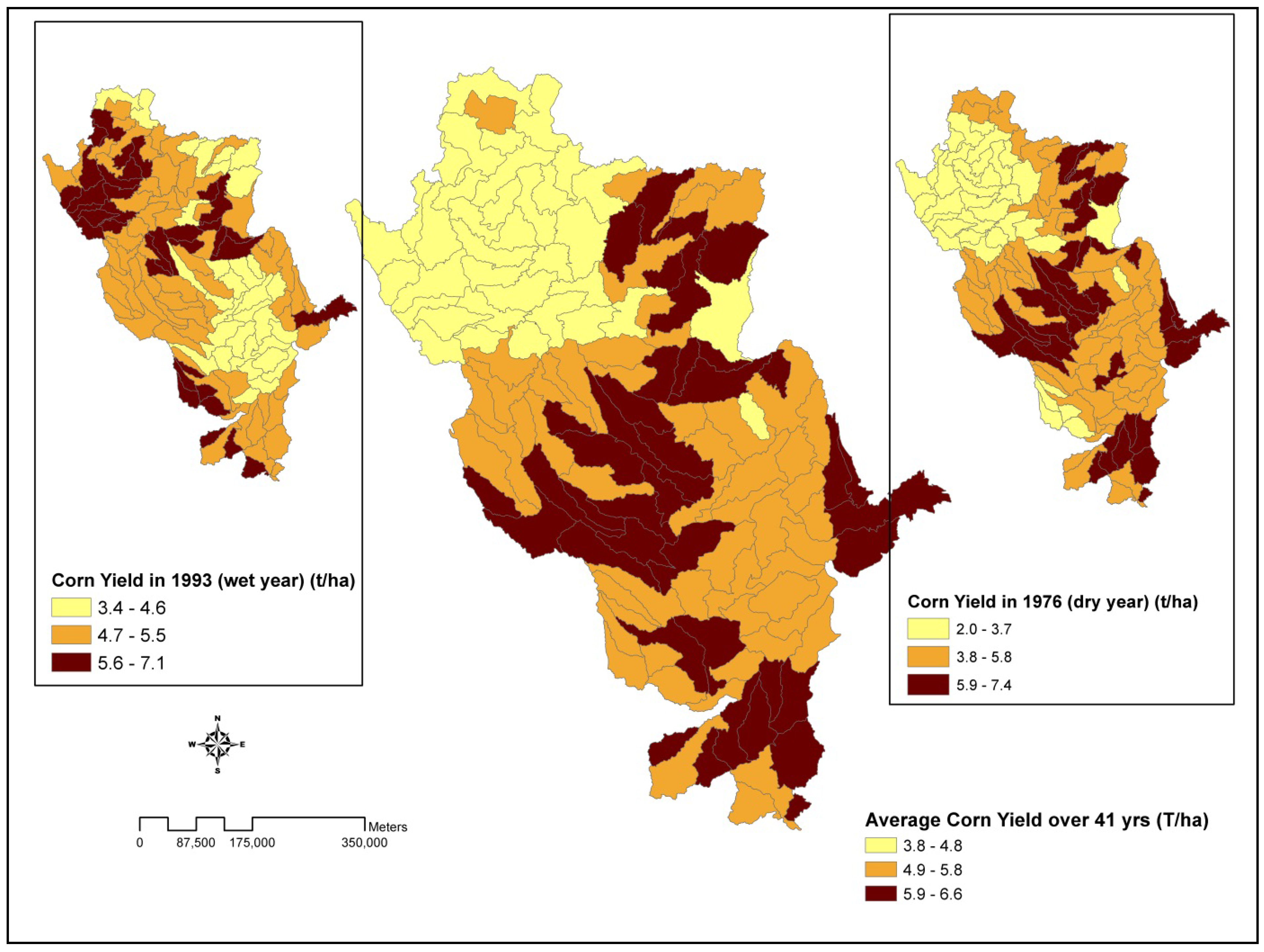
How will extreme events affect crop yields and water availability and quality?

(3)

What are the possible water quality effects associated with increases in production of different kinds of biomass?

(4)

What agricultural practices might help reduce water use or minimize water pollution associated with biomass production?

2. Materials and Methods

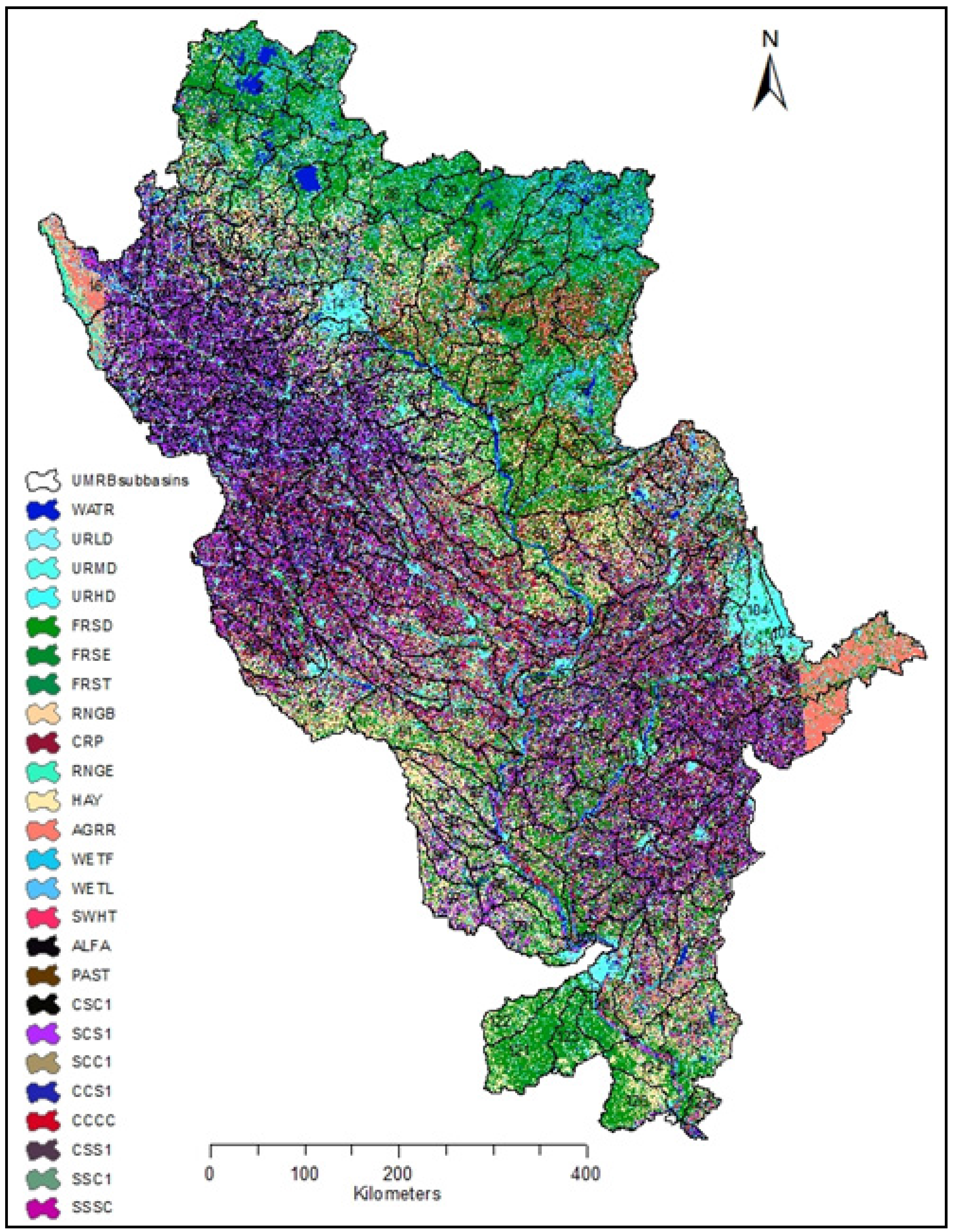
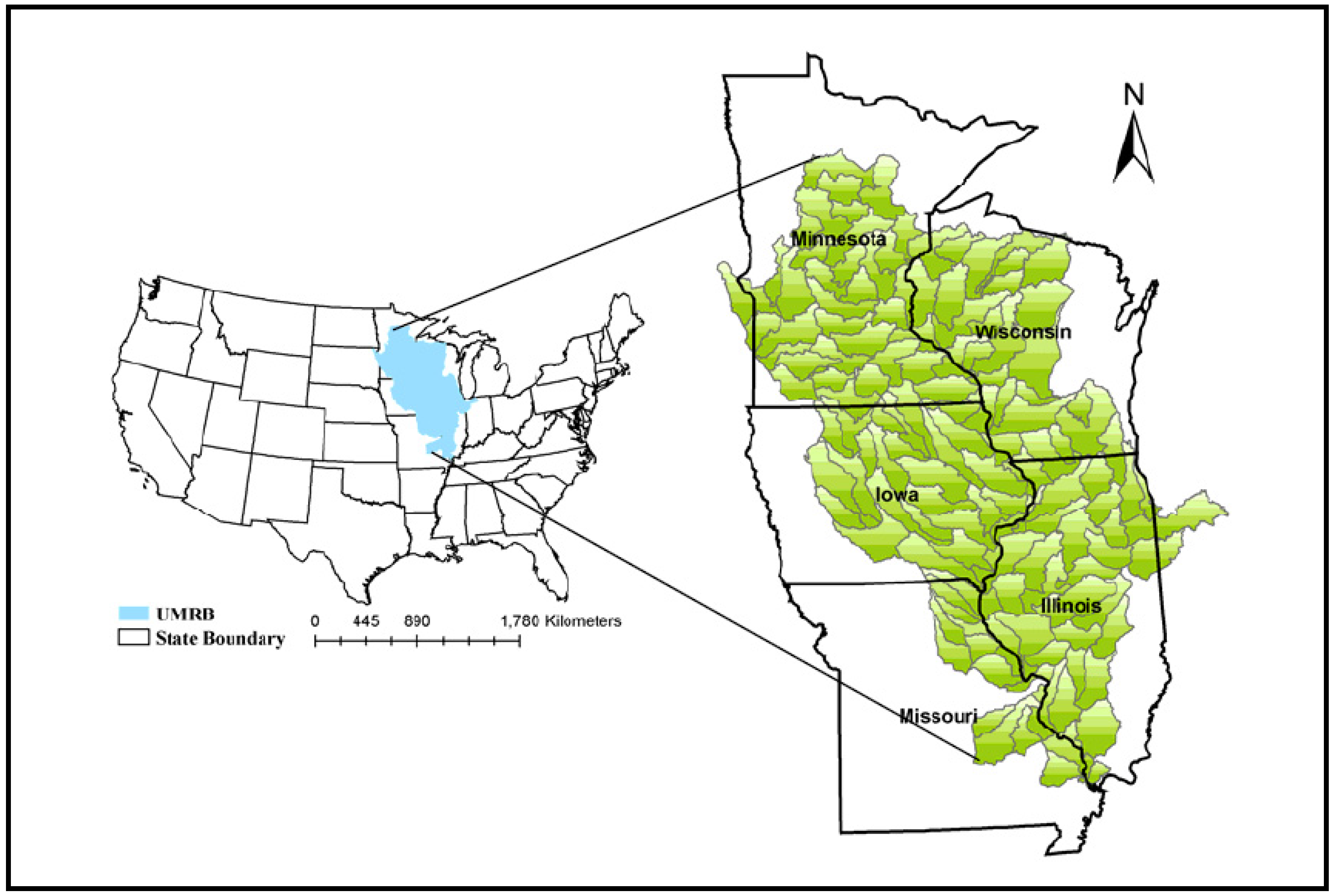
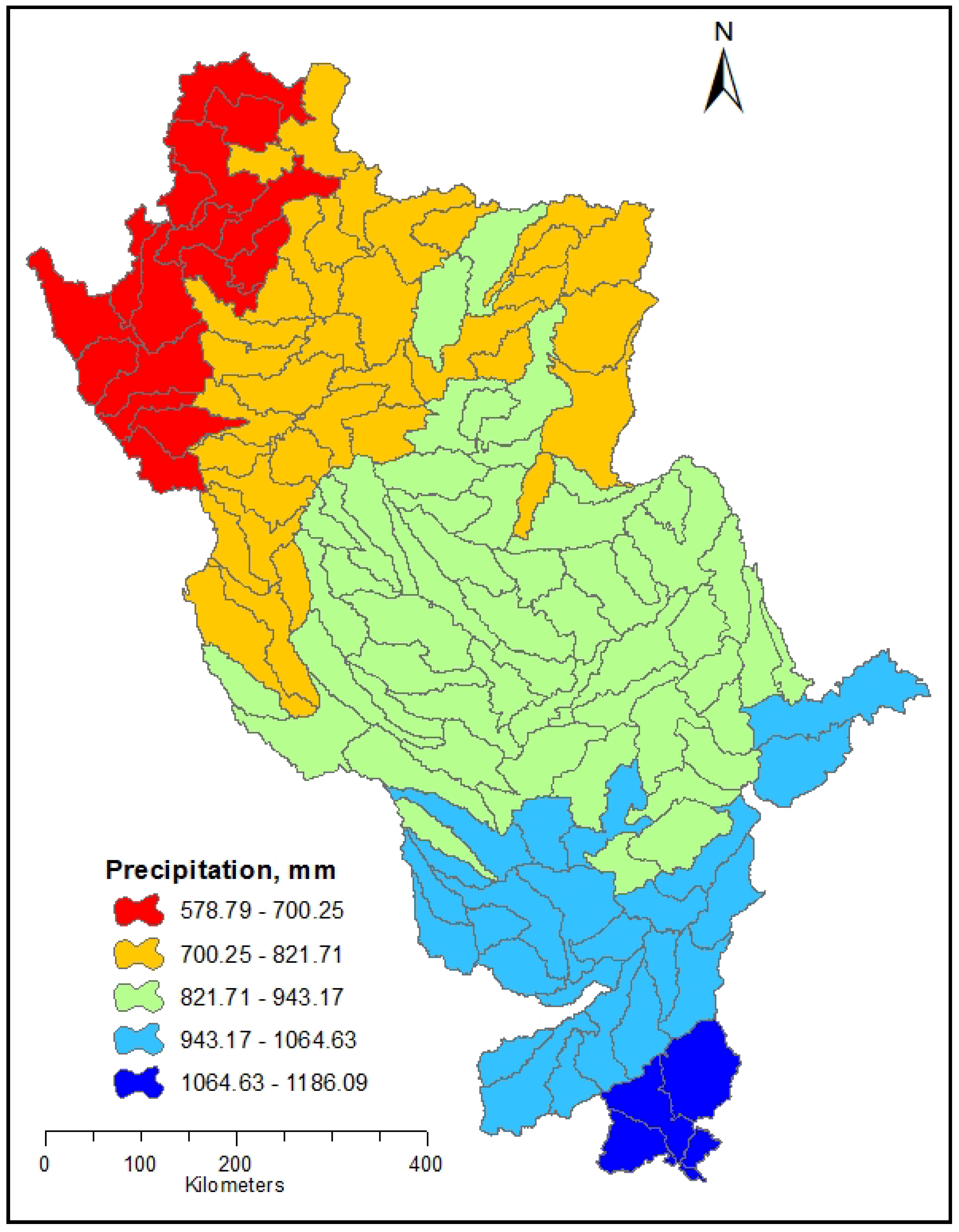
2.1. Study Area

The Upper Mississippi River Basin (UMRB) was selected to model the environmental impacts of biofuels expansion strategies under a variable climate and identify strategies that will help reduce the undesirable impacts in the biofuels supply chain. The UMRB was selected because it is a major corn producing watershed in the US producing about 43% of the total corn produced in the country [23]. As a result, the UMRB is representative of many potential concerns associated with ethanol production, including its association with major water quality issues such as the hypoxia in the Gulf of Mexico. Furthermore, the United States Congress recognizes the Upper Mississippi River System as an unique water body in the nation due to its “nationally significant ecosystem” and “nationally significant commercial navigation system” [27]. Moreover, more than 30 million residents living in the region relies heavily on the river for their public and industrial water supplies and other water uses [28].

The UMRB (Figure 1) extends 190,000 square miles (492,098 km²) across the upper Midwestern United States starting at the headwaters of the Mississippi River (Lake Itasca) in upper Minnesota and extending southward till it meets the Ohio River near Cairo, Illinois. The basin includes large parts of Illinois, Iowa, Minnesota, Missouri, and Wisconsin, and small areas of Indiana, Michigan, and South Dakota.

Cultivated cropland is the dominant landcover covering over 52 percent of the basin, majority of it being in northeastern and central Iowa and southern Minnesota. Corn and soybean are the primary crops grown in this region followed by wheat and hay as significant other crops. Corn production from this region has been estimated to account for 43 percent of harvested corn grain in the United States while soybean production accounts for 37 percent of the national soybean production [23]. Other dominant landcover types includes forests which occupy 20 percent of the area, most of which is located in the northern parts of the basin (Minnesota and Wisconsin) and in the southern tip of the basin (Missouri), pasture and hayland covers 9 percent of the area, and rangeland, water, wetlands, horticulture, and barren land together account for about 11 percent of the area [29].

Figure 1. Location of Upper Mississippi River basin.

Figure 1. Location of Upper Mississippi River basin.

The soil type within the basin range from heavy, poorly drained clays to light, well-drained sands, with majority being silty loam and loam soils. Topography of the region is characterized by flat to gently rolling terrain, with with an average elevation of 300 m. Precipitation generally increases from north to south. Average annual precipitation of 900 mm occurs mostly between April and October. The average daily minimum and maximum temperatures during crop growth seasons within the watershed ranges from 12.8 to 16.7 °C in the north and 18.1 °C to 22.6 °C in the south [30].

2.2. Model Description

SWAT is a continuous-time, long-term, distributed parameter model [31]. Major model components include weather, hydrology, erosion/sedimentation, soil temperature, plant growth, nutrients, pesticides, bacteria, agricultural management, stream routing and pond/reservoir routing [32]. SWAT divides a watershed into smaller areas called subbasins that are connected by a stream network. Each subbasin is further divided into hydrologic response units (HRUs), which are unique combinations of land cover, slope, and soil type and simulates surface and subsurface flow, sediment generation and deposit, and nutrient movement and fate through the watershed system. As a physically based hydrological model, SWAT requires a great deal of input data in order to derive parameters that control the hydrologic processes in a given watershed. Major input datasets include weather, hydrography, topography, soils, land use/land cover data, and management practices.

The Soil and Water Assessment Tool (SWAT) was selected as the simulation tool for assessing the hydrological water footprint of advanced biomass feedstock due to its established technical capabilities, widespread use, comprehensive representation of watershed processes, and efficient computational execution. The model uses topography, soils, precipitation, plant growth, and crop management information to form a complete deterministic representation of the hydrology and water quality of a watershed. Furthermore, SWAT is a public domain model and has been applied extensively to support water quality and Total Maximum Daily Load (TMDL) planning throughout the United States. In addition, there have been some prior applications of SWAT for hydrology and nutrient simulation in the UMRB [28,31] that were available as a starting foundation for the modeling efforts and focus of this study.

2.3. UMRB SWAT Model

For this study we used the UMRB SWAT model from a previous study by a co-author [26] that was developed using the 8 digit USGS Hydrologic Unit code (HUCs), the National Hydrography Dataset (NHD), and 90 m (3-arc second) DEM data to define watershed and topographic parameters. Landuse data was generated from the Cropland Data Layer (CDL) [33] and the 2001 National Land Cover Data (NLCD 2001) [34] as illustrated in Figure 2.

STATSGO (USDA-NRCS, 1995) 1:250,000 scale map was used and all soil properties (e.g., soil texture, bulk density, available water capacity, saturated conductivity, soil albedo, and organic carbon) needed for the SWAT model were extracted from this layer. Management information was included in the form of tillage practices and fertilizer and manure applications. Tillage practice information was obtained at the county level from the Conservation Technology Information Center [35] using the regional data from 2004. Manure application rates were estimated from the livestock data of the 2002 Census of Agriculture and only the agricultural land use received manure applications. Long-term historical weather inputs from 1960 to 2001 at 2.5-min (~4 km) resolution for the UMRB SWAT model was generated using a methodology developed by combining daily observations from the National Climatic Data Center (NCDC) digital archives with maps from the Parameter-Elevation Regressions on Independent Slopes Model (PRISM) [36].

The UMRB SWAT model consists of a total of 131 8-digit subwatersheds ranging in size from 900 to 8500 sq. km and a total of 14,568 unique Hydrologic Response Units (HRUs) by using a threshold operation of 5% for Landuse, 10% for Soil and 5% for slope [37]. Evaluation of the UMRB SWAT model for hydrology and crop growth by Srinivasan et al., 2010 [37] yielded satisfactory results across the watershed making it suitable to future studies on estimating both water quantity and quality impacts due to landuse changes for biofuels under a variable climate. For the current study the UMRB SWAT model by Srinivasan et al., 2010 [37] was evaluated with the SWAT 2009 version. At the downstream most USGS stream gauge located on the Mississippi River at Grafton, Illinois the annual and monthly Nash-Sutcliffe coefficient hydrology was 0.72 and 0.62 respectively; annual and monthly R² (co-efficient of determination) was 0.87 and 0.7 respectively; annual and monthly PBIAS (Percent Bias) of 3.35 and −5 percent respectively. Evaluation of total nitrogen (TN) at the same site yielded an annual and monthly Nash-Sutcliffe coefficient of 0.61 and 0.53 respectively; annual and monthly R² (co-efficient of determination) was 0.76 and 0.53. This was consistent with results reported from earlier studies.

Figure 2. Landuse map for the Upper Mississippi River Basin (UMRB).

Figure 2. Landuse map for the Upper Mississippi River Basin (UMRB).

2.4. Scenario Development

In order to assess the spatio-temporal impacts of alternative potential future conditions within the UMRB, such as increased corn production or replacement of corn with other feedstock like switchgrass, SWAT model for a baseline scenario with “current” conditions was first established, to which the results of “future” condition model runs were compared. 15 different scenarios (Table 1) resulting from changes in land use or cropping conditions, management practices, and climate variation were analyzed for this study. These scenarios included:

Table 1. Scenarios for biofuel expansion.

Scenarios	Description	Crop Rotation	Stover Harvest Rate (%)	Management Practices	Cropland Replaced with Switchgrass (%)
Baseline		Corn-Soybean	0	Conventional Till	0
(A) Changes in Landuse or Cropping Conditions
A1	(i) Yield Comparison	Regular Continuous Corn	0		0
A2		High yielding Continuous Corn	0		0
A3	(ii) Landuse Change for Biofuel Expansion	Corn-Soybean	0		25
A4		Corn-Soybean	0		50
A5		Corn-Soybean	0		75
A6		Corn-Soybean	0		100
(B) Changes in Management Practices
B1	(i) Residue Removal Rates	Continuous Corn	25		0
B2		Continuous Corn	50		0
B3		Continuous Corn	75		0
B4	(ii) Sustainable corn-soybean management	Continuous Corn	0	No-Till	0
B5		Continuous Corn	25	No-Till	0
B6		Continuous Corn	50	No-Till	0
B7		Continuous Corn	75	No-Till	0
(C) Climate Variability
C1	Precipitation increased by 10%	Corn-Soybean	0		0
C2	Temperature increased by 2 °C and precipitation decreased by 10%	Corn-Soybean	0		0

Table 1. Scenarios for biofuel expansion.

Scenarios	Description	Crop Rotation	Stover Harvest Rate (%)	Management Practices	Cropland Replaced with Switchgrass (%)
Baseline		Corn-Soybean	0	Conventional Till	0
(A) Changes in Landuse or Cropping Conditions
A1	(i) Yield Comparison	Regular Continuous Corn	0		0
A2		High yielding Continuous Corn	0		0
A3	(ii) Landuse Change for Biofuel Expansion	Corn-Soybean	0		25
A4		Corn-Soybean	0		50
A5		Corn-Soybean	0		75
A6		Corn-Soybean	0		100
(B) Changes in Management Practices
B1	(i) Residue Removal Rates	Continuous Corn	25		0
B2		Continuous Corn	50		0
B3		Continuous Corn	75		0
B4	(ii) Sustainable corn-soybean management	Continuous Corn	0	No-Till	0
B5		Continuous Corn	25	No-Till	0
B6		Continuous Corn	50	No-Till	0
B7		Continuous Corn	75	No-Till	0
(C) Climate Variability
C1	Precipitation increased by 10%	Corn-Soybean	0		0
C2	Temperature increased by 2 °C and precipitation decreased by 10%	Corn-Soybean	0		0

(a)

Changes in landuse or cropping conditions

(i)

Yield intensification: Changes in cropping conditions were simulated by a scenario with continuous corn plantation (A1) and a yield intensification scenario (A2) in which all the area within the basin having corn-soybean (approximately 125,000 sq. km) rotation under the baseline scenario was simulated as continuous corn of regular variety and a high yielding variety respectively.

(ii)

Landuse change for biofuel expansion: Changes in landuse was simulated by scenarios (A3, A4, A5, A6) depicting gradual spatial conversion of the current cropland to dedicated energy grasses such as switchgrass. The replacement of cropland with switchgrass ranged from 25% to 100% and helped to identify the point where the replacement will have significant impact and thereby helped to determine an optimal land allocation that maximizes net returns with minimal environmental impacts.

(b)

Changes in management practices

(i)

Residue removal rates: Corn stover is being considered as an attractive sources of biomass in a way that agricultural residue is utilized while the harvested grain is still used for feed. More than 90% of the corn stover in the US is left on the fields; about 5% is baled for animal feed and bedding, and less than 1% is used for industrial processing [38]. This amounts to 100–150 million tons of corn stover, in the Midwest alone, left on fields for erosion control and nutrient/carbon build-up in the soils [39]. The benefits of corn stover removal are: (1) higher ethanol production rate per unit arable land; (2) energy recovery from lignin-rich fermentation residues; (3) less competition for food and feed; (4) lower nitrogen related environmental burdens from the soil such as decreased N₂O from the soil, reduced inorganic nitrogen losses due to leaching. The disadvantages of corn stover removal are: (1) a lower replenishment rate of soil organic carbon; (2) higher soil erosion rates due to the lack of ground cover; (3) higher fuel consumption in harvesting corn stover unless technology is improved to harvest both grain and stover in a single pass [38]. Under this scenario, we ran simulations (B1, B2, B3) with different corn stover removal rates ranging from 25% to 75% under baseline tillage conditions with no cover crops.

(ii)

Sustainable corn-soybean management: Sustainable reduced tillage production systems sometimes help to reduce the adverse effects of removal of agricultural residues. Powers et al. [40] found that even with 75% removal of corn stover, practicing no-till system produced 3% less erosion compared to corn-soybean conventional tillage system. Therefore we simulated scenarios (B4, B5, B6, B7) resulting from different percentages of corn stover removal (25%–75%) under no-till conditions with no cover crops.

(c)

Climate variability

• Climate variability (Figure 3 and Figure 4) and change can impact crop yield, hydrology and water quality of a region. On analyzing the weather pattern in the UMRB from 1960 to 2001, it was determined that 1993 was the wet year and 1976 was the dry year.

Consequently, both corn yield (Figure 4) and hydrology of the UMRB (Table 2) shows significant variability in both wet and dry years. Therefore it seemed essential to simulate hydrological and water quality effects of biofuel crop growth under climate induced stress. Hence, temperature was increased and rainfall was reduced to simulate drought condition, to an extent, which will help to estimate the soil moisture deficit and the irrigation requirements to maintain the crop growth. A scenario (C1) was simulated with just precipitation reduced by 10% and then another scenario (C2) was simulated with a combination of increased temperature by 2 degrees and decreased precipitation by 10%. The basis for increasing the temperature and decreasing the precipitation was the variation in annual weather pattern from which it was determined that the possible worst climate scenario in this region will be governed by an increase in temperature by 2 °C and a decrease in rainfall by 10%.

Figure 3. Spatial Variation of annual average precipitation (over 1960–2001) across UMRB watershed.

Figure 3. Spatial Variation of annual average precipitation (over 1960–2001) across UMRB watershed.

Figure 4. Spatial variation of corn yield (t/ha).

Figure 4. Spatial variation of corn yield (t/ha).

Table 2. Comparison of Hydrologic Components between Baseline, Wet (1993) and Dry (1976) Years. ET = evapo-transpiration.

Year	Precipitation (mm)		ET (mm)		Water Yield (mm)		Surface Water Yield (mm)		Groundwater Yield (mm)
	Average	% Change over Baseline	Average	% Change over Baseline	Average	% Change over Baseline	Average	% Change over Baseline	Average	% Change over Baseline
Baseline	850.1	0	617.7	0	200.00	0	105.0	0	95.0	0
Wet year (1993)	1100.0	29.4	605.2	−2.0	502.7	151.4	311.9	197.1	190.8	100.9
Dry year (1976)	569.1	−33.06	546.0	−11.6	143.8	−28.1	48.3	−54.0	95.5	0.6

Table 2. Comparison of Hydrologic Components between Baseline, Wet (1993) and Dry (1976) Years. ET = evapo-transpiration.

Year	Precipitation (mm)		ET (mm)		Water Yield (mm)		Surface Water Yield (mm)		Groundwater Yield (mm)
	Average	% Change over Baseline	Average	% Change over Baseline	Average	% Change over Baseline	Average	% Change over Baseline	Average	% Change over Baseline
Baseline	850.1	0	617.7	0	200.00	0	105.0	0	95.0	0
Wet year (1993)	1100.0	29.4	605.2	−2.0	502.7	151.4	311.9	197.1	190.8	100.9
Dry year (1976)	569.1	−33.06	546.0	−11.6	143.8	−28.1	48.3	−54.0	95.5	0.6

3. Results and Discussion

The SWAT model for the UMRB was executed for the available input climate record, 1960–2001, with simulations under conditions of the increased corn production and yields, energy grass intervention, different residue removal rates, sustainable corn-soybean management, and variable climate. Separate model runs were performed for each of the scenarios, and the model results were analyzed to provide changes (Table 3) in water quantity and quality from the baseline simulation.

Table 3. Percent changes in Water Yield, ET, Sediment Yield and Total Nitrogen Load under different scenarios.

Scenarios	% Change from Baseline
	Precipitation	ET	Water Yield	Surface Water Yield	Groundwater Yield	Sediment Load	Total Nitrogen Load
Baseline	0	0	0	0	0	0	0
A1	0	0.2	−0.5	0	−1	1.6	−1.5
A2	0	0.2	−0.5	0	−1	1.6	−1.5
A3	0	0.7	−1.4	0	−2.9	7.6	−10.1
A4	0	−5.2	9.4	−0.8	20.6	−96.1	−69
A5	0	−5.2	9.4	−0.8	20.6	−96.1	−69
A6	0	−4.8	10.2	−0.1	21.6	−95.6	−70.4
B1	0	2.8	−6.4	0	−13.5	−3.1	−9.1
B2	0	3.7	−8.2	0	−17.3	5.9	−13.5
B3	0	4.4	−9.8	0	−20.6	26.5	−5.6
B4	0	−0.2	0.4	0	0.9	−2.6	−2.1
B5	0	2.6	−6	0	−12.5	−5.5	−12.5
B6	0	3.5	−6	0	−16.6	3.2	−12.5
B7	0	3.5	−7.9	0	−16.6	3.2	−19.6
C1	−10	−2.1	−31.9	−41.2	−21.5	−42.3	−37.5
C2	−10	1.2	−41.6	−57.1	−24.6	−50.3	−48.4

Table 3. Percent changes in Water Yield, ET, Sediment Yield and Total Nitrogen Load under different scenarios.

Scenarios	% Change from Baseline
	Precipitation	ET	Water Yield	Surface Water Yield	Groundwater Yield	Sediment Load	Total Nitrogen Load
Baseline	0	0	0	0	0	0	0
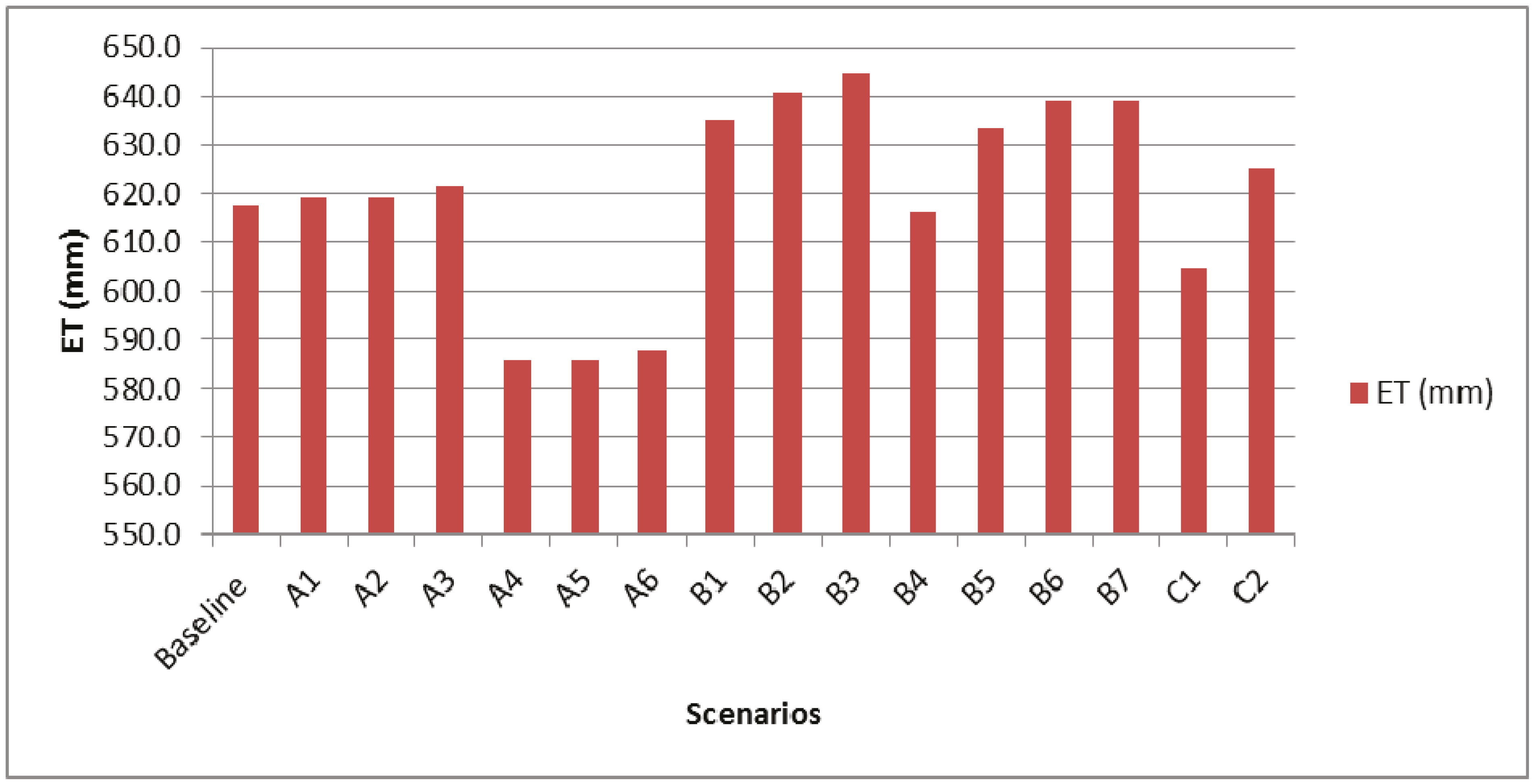
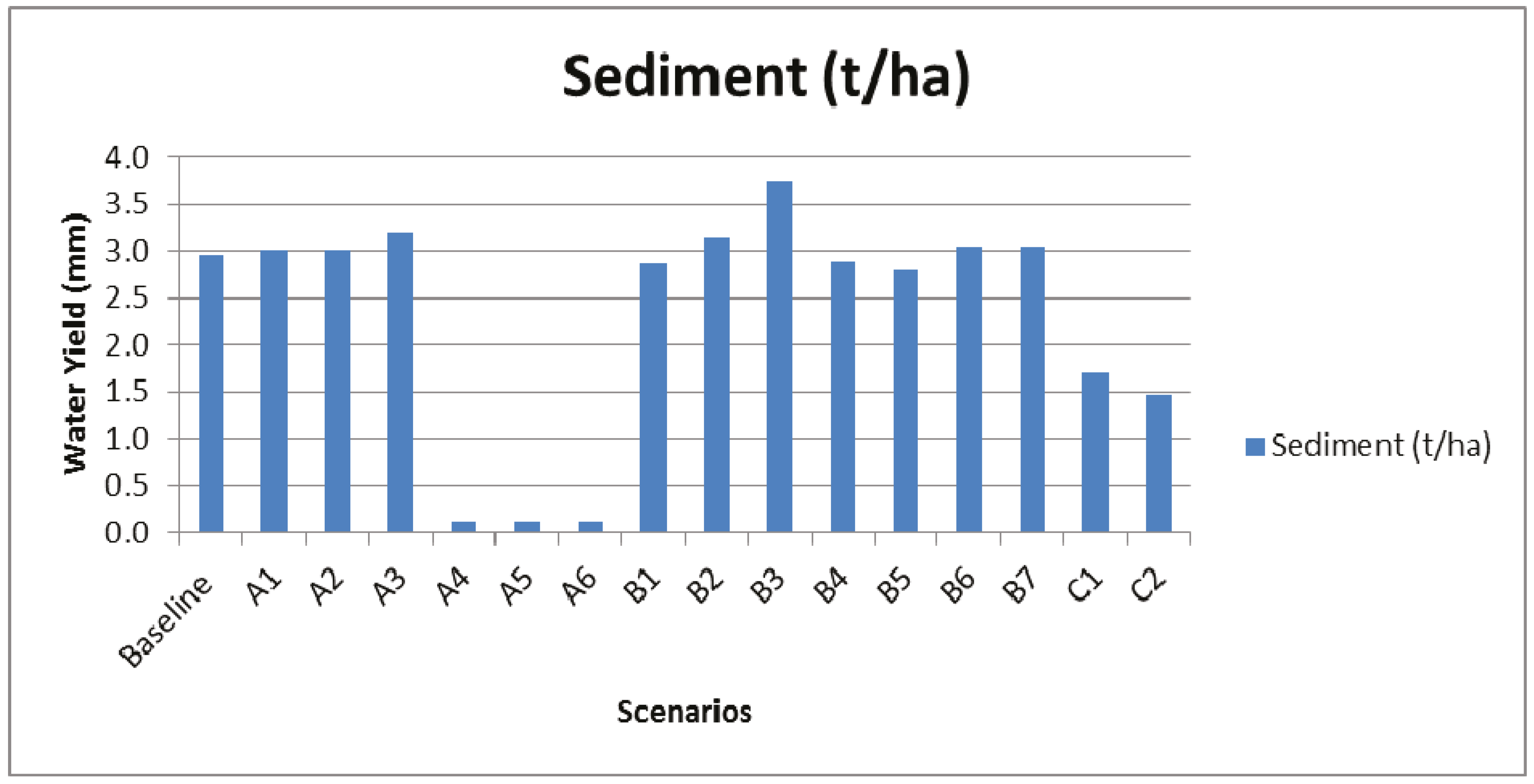
A1	0	0.2	−0.5	0	−1	1.6	−1.5
A2	0	0.2	−0.5	0	−1	1.6	−1.5
A3	0	0.7	−1.4	0	−2.9	7.6	−10.1
A4	0	−5.2	9.4	−0.8	20.6	−96.1	−69
A5	0	−5.2	9.4	−0.8	20.6	−96.1	−69
A6	0	−4.8	10.2	−0.1	21.6	−95.6	−70.4
B1	0	2.8	−6.4	0	−13.5	−3.1	−9.1
B2	0	3.7	−8.2	0	−17.3	5.9	−13.5
B3	0	4.4	−9.8	0	−20.6	26.5	−5.6
B4	0	−0.2	0.4	0	0.9	−2.6	−2.1
B5	0	2.6	−6	0	−12.5	−5.5	−12.5
B6	0	3.5	−6	0	−16.6	3.2	−12.5
B7	0	3.5	−7.9	0	−16.6	3.2	−19.6
C1	−10	−2.1	−31.9	−41.2	−21.5	−42.3	−37.5
C2	−10	1.2	−41.6	−57.1	−24.6	−50.3	−48.4

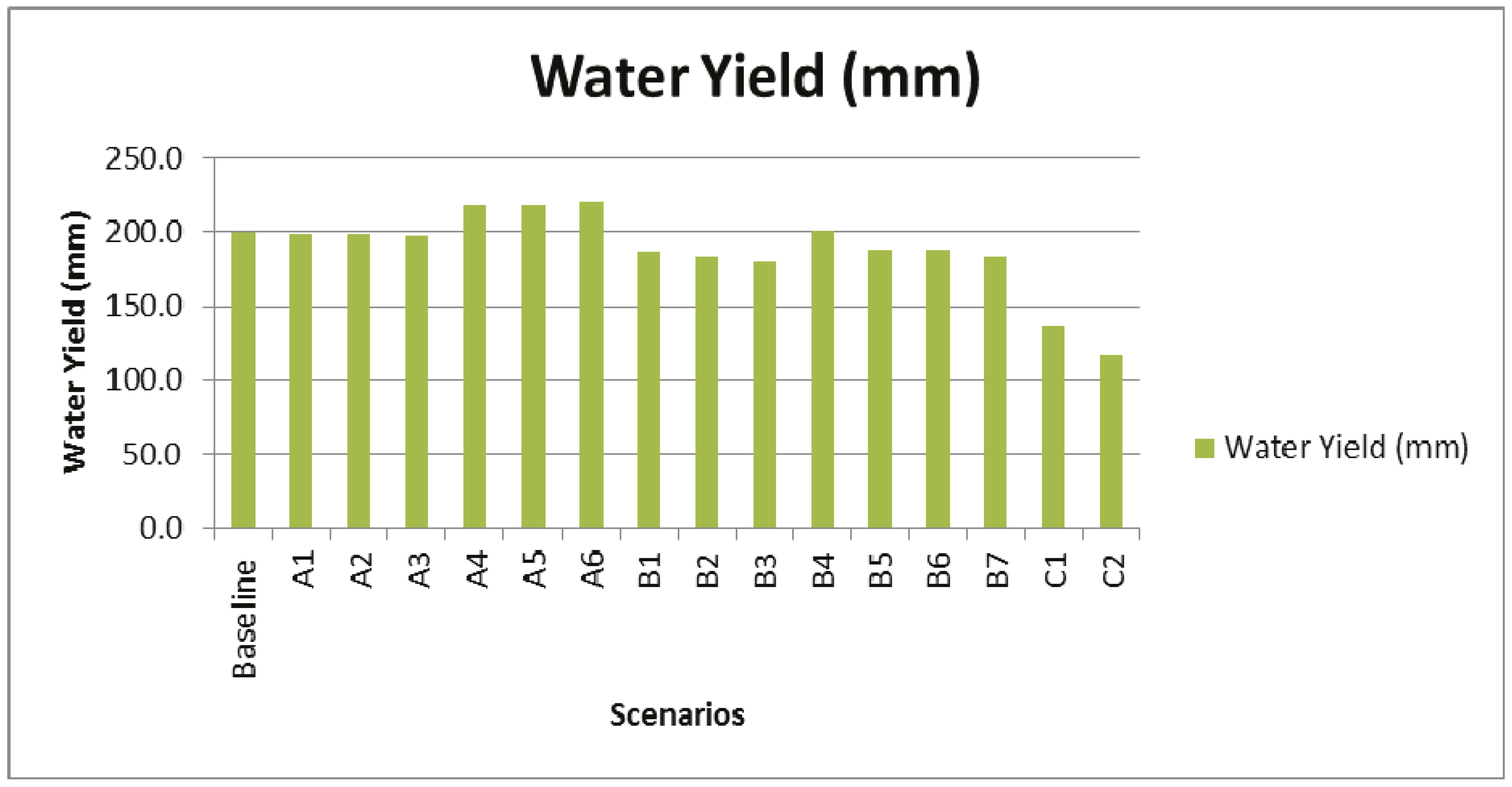
3.1. Impacts on Water Yield and Water Consumption

Figure 5 and Figure 6 shows the annual average annual water yield and water consumption at the basin scale for the 15 different scenarios during the 42-year simulation period. As shown, yield intensification through planting regular and intense yield variety of continuous corn on all the agricultural land that had corn-soybean rotation (scenario A1 and A2) in the baseline condition did not result in any significant change in the water yield and water consumption through evapo-transpiration (ET) as shown by a 0.5% (0.9 mm) decrease in water yield and 0.2% (1.32 mm) increase in evapo-transpiration. However, significant changes in landuse through spatial conversion of the current cropland to switchgrass resulted in changes in water yield and water consumption. Converting 25% of current cropland to switchgrass (scenario A3) did not impact the water yield and water consumption much by decreasing the water yield of the basin by 1.5% and increasing ET by 0.6% and decreasing ground water yield by 3% (Table 3). But, replacing 50%–100% cropland with switchgrass (scenarios A4–A6) resulted in 10% increase in water yield and a 5% decrease in water consumption through ET, very little reduction in surface water yield by 0.8%, but increased ground water yield by as much as 20% (Table 3).

Simulating progressive removal of corn stover residues (scenarios B1-B7) also resulted in changes in water yield and water consumption at the basin scale. As seen from Table 3, a 25% removal of corn stover reduces water yield by 6% with a 2.5% increase in evapo-transpiration. A 50%–75% corn stover removal decreases water yield by around 5%–10% and increases ET by 3%–4%. This may be attributed to the effect of the residues on the ground; as more residues are removed, evaporation from the soil increases thereby reducing the water yield. There was no change in the surface water yield under different corn stover removal rates, but ground water yield decreased by 12%–16% (Table 3).

Figure 5. Annual Average Water Yield at the watershed scale under the 15 different scenarios.

Figure 5. Annual Average Water Yield at the watershed scale under the 15 different scenarios.

Figure 6. Annual average water consumption through evapo-transpiration (ET) at the watershed scale under the 15 different scenarios.

Figure 6. Annual average water consumption through evapo-transpiration (ET) at the watershed scale under the 15 different scenarios.

In addition, climate variability also produced significant changes in water yield and ET. A 10% decrease in rainfall resulted in a 34% decrease in water yield, 21% decrease in ET, 40% decrease in surface water yield and 20% decrease in ground water yield. When a 10% decrease in precipitation was coupled with a 2 degree increase in temperature, water yield decreased by 44.5% and ET increased by 1.2%, surface water decreased by 50% and ground water decreased by 25% (Table 3).

3.2. Impacts on Soil Erosion and Sediment Control

Annual average sediment yield from the UMRB for the 15 scenarios (Table 1) are shown in Figure 7. As expected, landuse change impacts on sediment erosion through yield intensification (scenario A1-A2) by planting continuous corn did not produce much change in sediment loading as is indicated by a 1.5% (0.04 t/ha) increase. In addition, the impact of growing perennial grasses (scenarios A3-B6) as bioenergy crops on sediment erosion was also examined. Since perennial grasses do not need any tillage applications, it was observed that a gradual replacement of cropland with switchgrass by 25–50–75–100 percent resulted in significant decrease in sediment loadings. The decrease in sediment loading was only 7% when 25% of the cropland was replaced by switchgrass, however a 50%–100% replacement of cropland by switchgrass led to a decrease in sediment loading by 96%.

Figure 7. Annual average sediment load at the watershed scale under the 15 different scenarios.

Figure 7. Annual average sediment load at the watershed scale under the 15 different scenarios.

Impact of management practices on sediment erosion was analyzed by removing corn stover residues under both baseline tillage conditions and no-till conditions. It was observed that by removing 25% of the corn stover under both baseline tillage practices and no-till conditions (scenarios B1 and B5) reduced the sediment loadings by 3% (0.09 t/ha) and 5% (0.16 t/ha) respectively whereas 50%–75% corn stover removal (scenarios B2-B3) under baseline till conditions increases sediment loading by upto 25% as higher the corn stover removal rates, more exposed is the ground surface to erosion. However, when coupled with no-till farming, sediment loading was brought down over the baseline irrespective of the stover removal rate.

Furthermore, the effect of climate variability on sediment loadings was also examined as variable climate can affect both regional and local water quality through runoff containing sediments. It was seen that the sediment load decreased by as much as 40% when precipitation is decreased (scenario C1) and 50% when both precipitation and temperature is decreased (scenario C2).

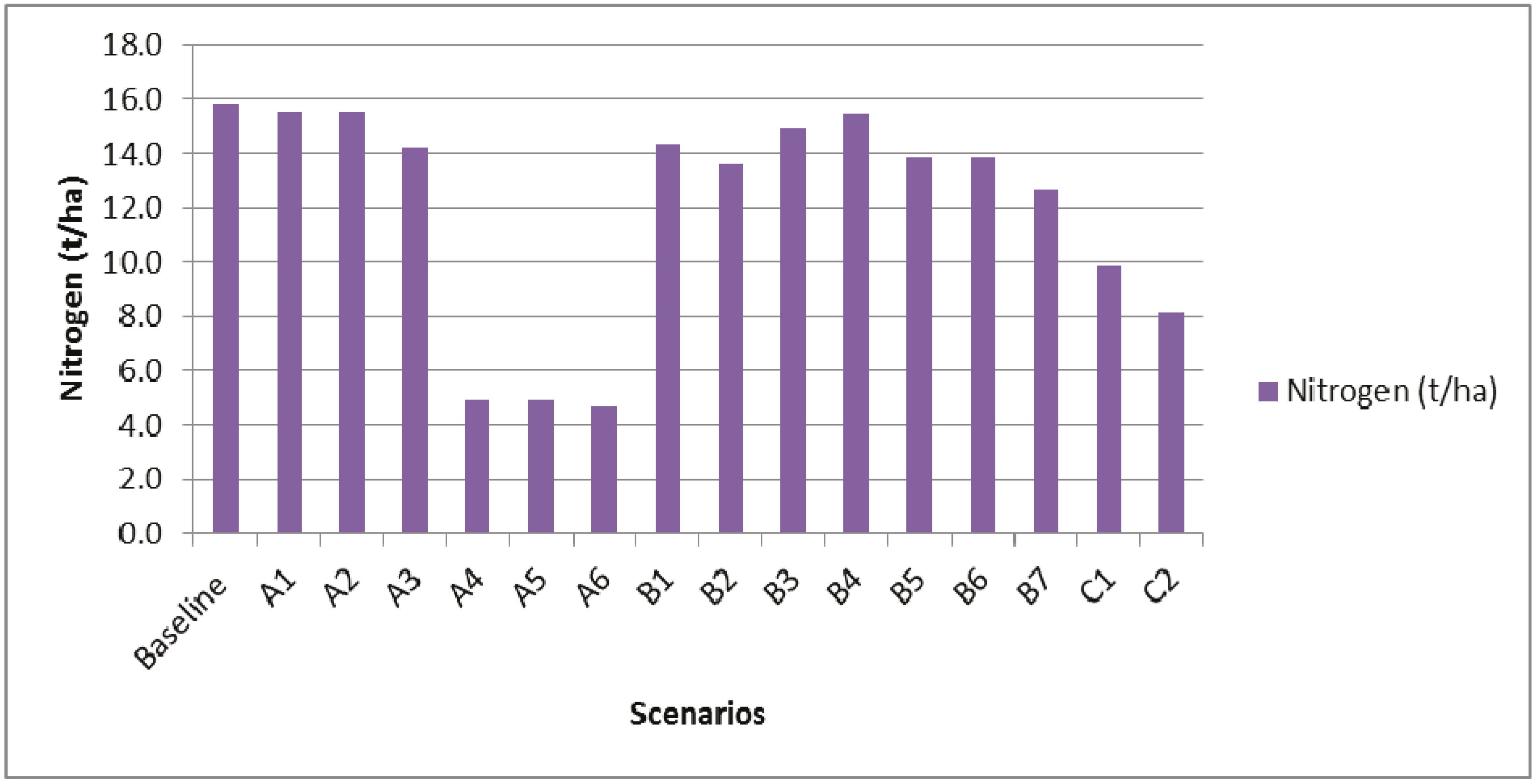
3.3. Impacts on Nutrient Loads

Annual average total nitrogen (TN) load under 15 different scenarios are shown in Figure 8. It was observed that yield intensification through planting continuous corn on all the agricultural land that had corn-soybean rotation (scenario A1) in the baseline condition did not lead to any significant change in total nitrogen (TN) load as shown by a 1.4% (0.22 kg/ha) decrease in TN. However landuse changes through gradual spatial conversion of the current cropland to switchgrass (scenarios A3-A6) resulted in a considerable decrease in TN loadings. This is due to the fact that switchgrass does not need additional fertilizers as corn. The decrease in TN loading was only 10% when 25% of the cropland was replaced by switchgrass, however a 50%–100% replacement of cropland by switchgrass led to a decrease in TN loading by as much as 70%.

Figure 8. Annual average total nitrogen load at the watershed scale under the 15 different scenarios.

Figure 8. Annual average total nitrogen load at the watershed scale under the 15 different scenarios.

Changes in management practices by removing corn stover residues progressively from 25% to 75% (scenarios B1-B7) also resulted in reduction of TN loadings. The reduction in TN loadings increased as less percentage of stover is removed i.e., TN loadings decreased more when 25% corn stover is removed than when 75% corn stover is removed. Removing corn stover under baseline till conditions reduced TN loadings by 5%–9% and by as much 20% under no-till conditions.

Climate variability also produced significant changes in total nitrogen loadings as observed in the wet and dry years. Therefore, a 10% decrease in rainfall in the future (scenario C1) may result in a 40% decrease in TN. Coupled with a 2 degree increase in temperature (scenario C2), TN decreased by around 50%.

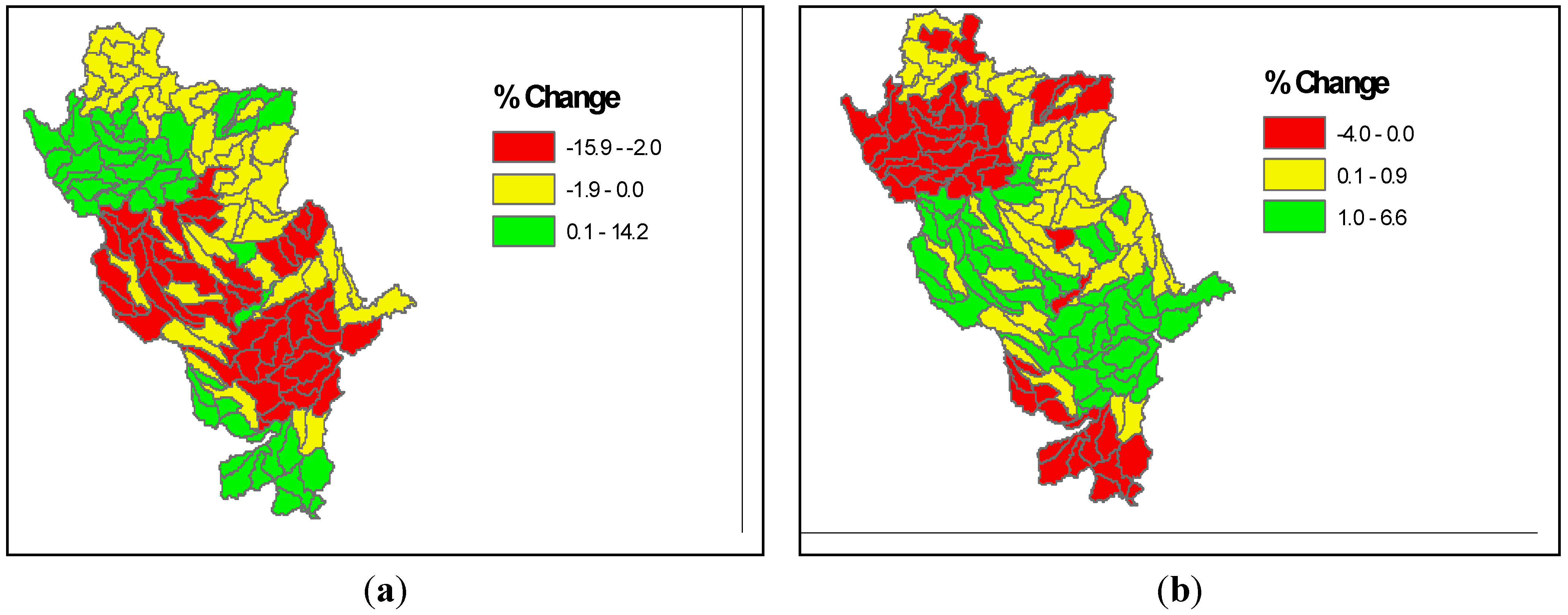
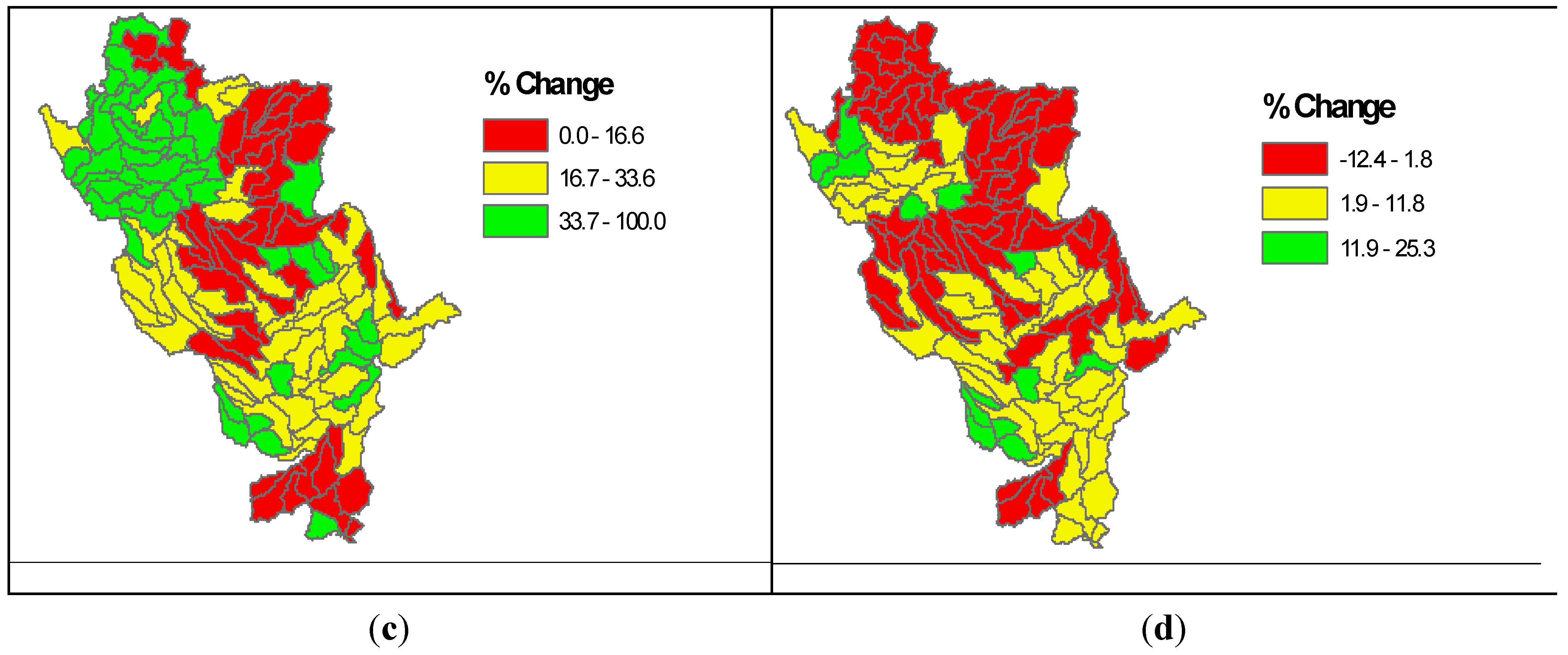
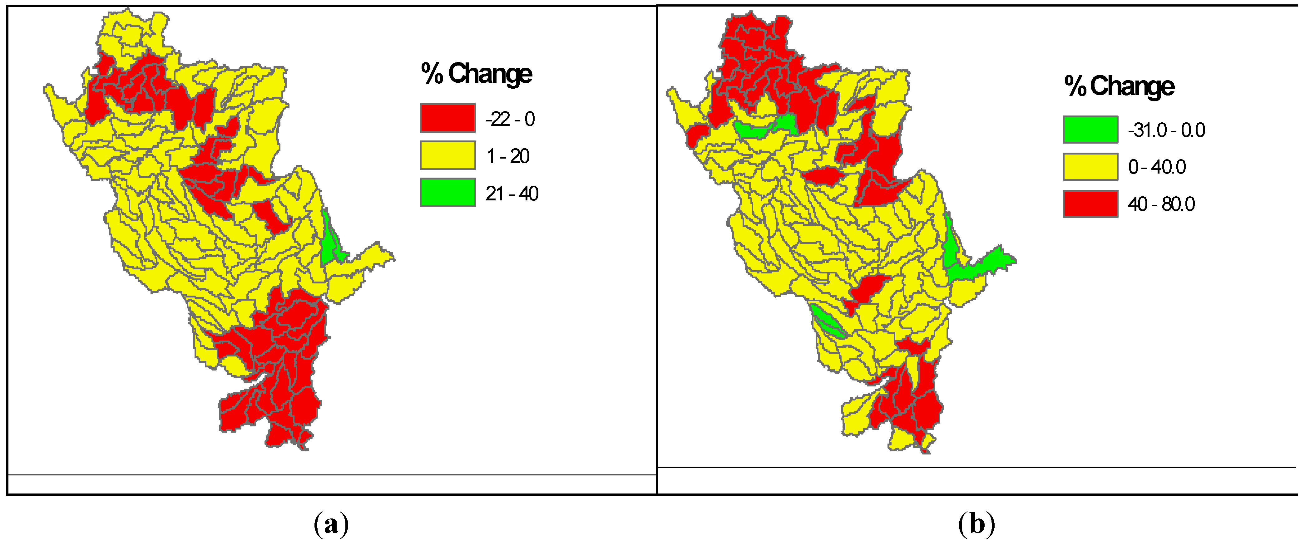
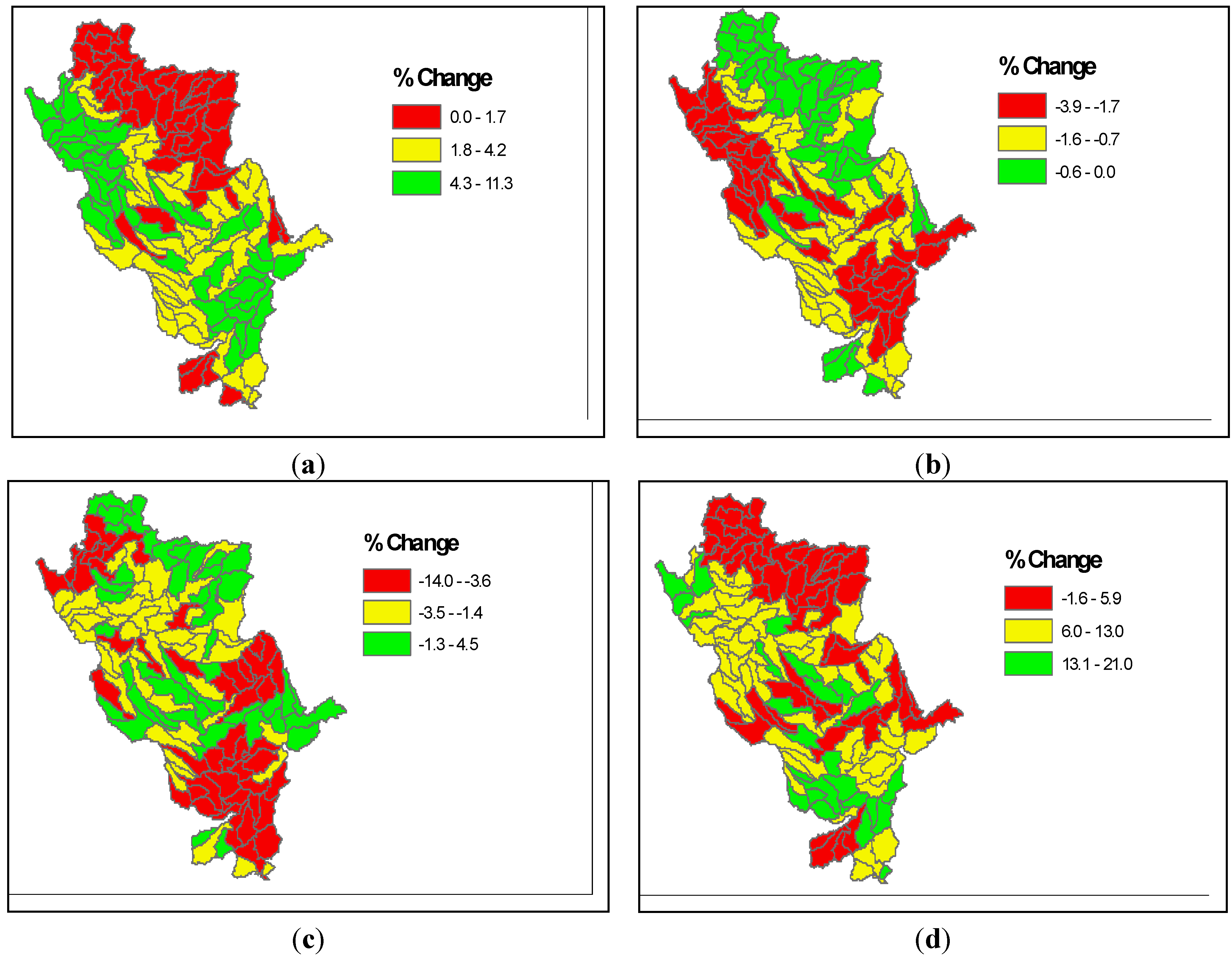
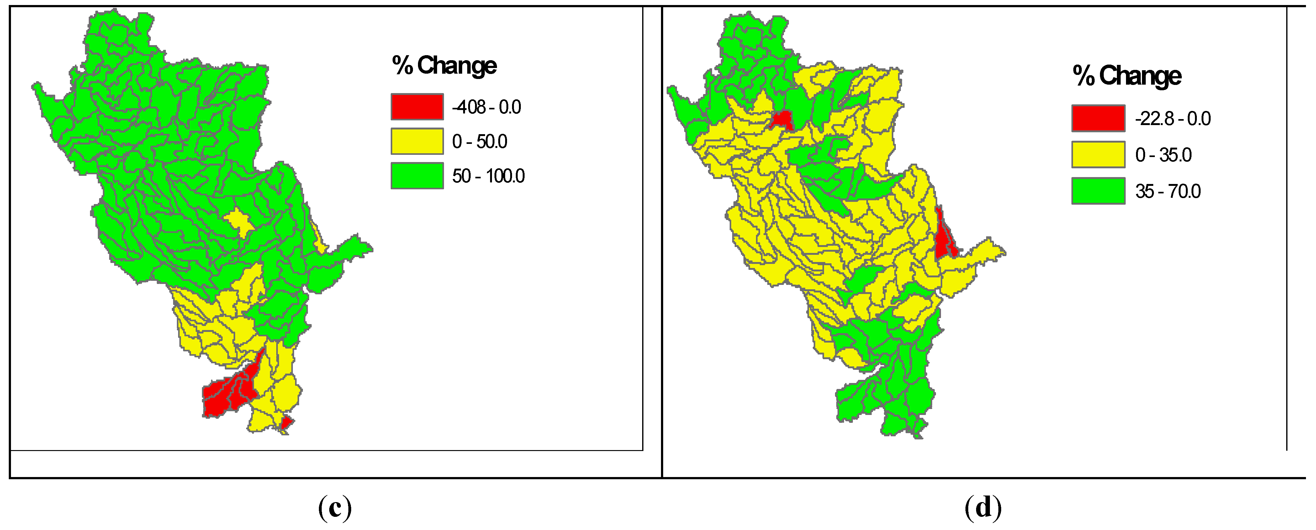
3.4. Spatial Impacts of Biofuel Production

Biofuel production under alternative landuse, management practices and climate variability will result in changes in the hydrology and water quality at the spatial scale in the UMRB. Moreover, some areas may be negatively impacted and implementation of conservation efforts for those areas will require identification of the areas that requires the Best Management Practices (BMPs) the most. Therefore, we created maps of the UMRB depicting areas that will be affected by dividing the basin into low, medium and high priority areas for water stress, sediment erosion and total nitrogen loading for each of the different scenario groups such as landuse change, management practices, and climate variability. We selected the most plausible scenarios amongst each group and analyzed the resulting spatial changes.

Landuse changes through yield intensification (scenarios A1-A2) by growing continuous corn do not have any significant impact on both the quantity and quality of water in the UMRB. However, progressive spatial conversion of 25%–100% of the cropland with switchgrass (scenarios A3-A6) resulted in significant improvement in the water quality of the UMRB with a 95% decrease in sediment erosion and 70% decrease in TN loadings. In addition the water yield and consumption increased by 10% and decreased by 5% respectively. But, changing 100% of the cropland to switchgrass is not viable and replacing 25% of the cropland resulted in insignificant changes in water yield and consumption and 7% increase in sediments. Therefore we selected the scenario where 50% of the cropland will be replaced with switchgrass (scenario A4) as the most viable amongst the landuse change scenarios for analyzing the spatial changes. Figure 9 shows the spatial changes in scenario A4 over the baseline scenario. As seen from the figure, under this scenario (A4), the increase in water yield is maximum in the subbasins towards the northwestern and southwestern part of the watershed whereas subbasins in the central part shows decrease in water yield or very little increase in water yield. Water consumption through evapotranspiration will decrease in the downstream most subbasins and northwestern subbasin whereas the central part of the watershed will experience an increase in the evapotranspiration. Sediment loadings will increase across the whole watershed, however subbasins from the northwestern part will contribute more towards the sediment loadings than the central or the southern part. Total nitrogen loadings varies significantly across the watershed with the northern and eastern subbasins contributing less whereas the southern and northwestern subbasins contributing more.

In addition, scenarios related to changes in management practices (B1-B7) may also result in an increase in water consumption by up to 5%, decrease in water yield by upto 10%, increase in sediment erosion by 3%–26% and decrease in TN loadings by 5%–20%. Similar to our selection in the landuse change scenarios, we selected scenario B4 (no corn stover removal with no-till practices) as the best option that has minimal negative environmental impact. However if corn stover needs to be used for biofuel generation then scenarios B1 and B4 are most plausible ones and scenario B3 (corn stover removal rate of 75% with baseline tillage practices) represents the most extreme one with maximum negative impact on the environment. Figure 10 shows the areas that may be impacted under scenario B4 and the hotspots (high priority areas) that may need conservation practices. Water Yield will increase across the whole watershed, with more increase towards the western and southern parts and less increase towards the northeastern part. Evapotranspiration will decrease across the whole watershed, with more decrease towards the western and southern parts and less decrease towards the northeastern part.

Figure 9. Spatial variation in the % change over baseline of: (a) Water Yield; (b) ET; (c) Sediment load; and (d) Total Nitrogen load from a 50% stover removal under no-till condition.

Figure 9. Spatial variation in the % change over baseline of: (a) Water Yield; (b) ET; (c) Sediment load; and (d) Total Nitrogen load from a 50% stover removal under no-till condition.

Figure 10. Spatial variation in the % change over baseline of: (a) Water Yield; (b) ET; (c) Sediment load; and (d) Total Nitrogen load from a 50% Switchgrass Adaptation (Scenario A4).

Figure 10. Spatial variation in the % change over baseline of: (a) Water Yield; (b) ET; (c) Sediment load; and (d) Total Nitrogen load from a 50% Switchgrass Adaptation (Scenario A4).

Finally, amongst the climate variability scenarios we selected the one with changes in both precipitation and temperature (scenario C2) to analyze the spatial impacts on both water quantity and water quality in the UMRB. Figure 11 shows that most of the watershed will experience a reduction in water yield and increase in water consumptions through ET due to decrease in precipitation and increase in temperature. Few isolated subbasins will show an increase in water yield and decrease in ET. Sediment loadings will increase across the whole watershed; however a few subbasins towards the south will experience a drastic reduction in sediment loadings. Similarly nitrogen loadings will also increase across the whole watershed except a few isolated ones.

Figure 11. Spatial variation in the % change over baseline of (a) Water Yield; (b) ET; (c) Sediment load; and (d) Total Nitrogen load from a 10% decrease in precipitation and 2 °C increase in temperature.

Figure 11. Spatial variation in the % change over baseline of (a) Water Yield; (b) ET; (c) Sediment load; and (d) Total Nitrogen load from a 10% decrease in precipitation and 2 °C increase in temperature.

4. Summary and Conclusions

Hydrologic modelling is data intensive but a powerful tool to communicate to stakeholders on water consumption and availability, sediment and nutrients loading, effects of climate variability, and strategies for reducing the impact of agriculture on the hypoxia in Gulf of Mexico. The focus of this paper is on modeling the interaction between land use, climate change, water resources and the environment in future large scale biofuel production systems and is founded on the hypothesis that water quantity and quality will be influenced by climate variability and bioenergy development (due to both crop mix and forest usage shifts plus the possible utilization of marginal lands). The Soil and Water Assessment Tool (SWAT) was applied to the Upper Mississippi River Basin to assess the long-term environmental impacts of biofuel expansion strategies under different scenarios resulting from landuse change, management practices and climate variability. Specifically this research addresses changes in the water demand and availability, soil erosion and water quality driven by both climate variability and biomass feedstock production in the Upper Mississippi River Basin. Comparison of all the scenarios demonstrates that the effects of bioenergy crop production under a variable climate will have important consequences for hydrometeorology in the watershed. Results show the UMRB is a region of relatively low water stress with tremendous potential for lignocellulosic ethanol production. However, within the basin there is considerable variability in rainfall with its northern parts being drier than its southern parts. Therefore water requirement per unit of biomass (fresh weight) for corn and switchgrass and also the corn and switchgrass yields varies spatially across the basin. In addition, a simulated rainfall decrease by 10% resulted in a reduction in water availability (or stream flow) by 20%–40% and when coupled with an increase in temperature by 2 °C, the reduction was 70%. In addition, continuous corn and corn intensification did not impact the hydrology variables significantly indicating that corn intensification is an adequate strategy for biofuels expansion. However planting continuous corn may not be a feasible option as it can lead to a significant decrease in soybean production, thereby impacting soybean supply, prices and soybean based biodiesel production. Also, conservative stover removal rate of 25% is considered to be “safest” option; a 50% or 75% of corn stover removal increased N-load and sediment yield (erosion) significantly. However, a 50% stover removal rate could be considered if coupled with no-till, but a watch-out for nitrogen loading has to be integrated with this strategy. More options could be considered between the 25% and 50% stover removal rates to gather an optimum level of sediment and nutrient loading rates. Furthermore, increasing land use under switchgrass (from 25% replacement of corn to 100% replacement was considered) progressively increased the water availability (stream flow) in the watershed. Even with a 25% land use change into switchgrass from corn reduced soil erosion by 95% and N-loading by 60%. Therefore, integrating switchgrass into the agricultural land use could serve the dual purpose of biomass expansion as well as reducing hypoxic conditions in the Gulf of Mexico.

To develop adaptive policies for watershed management and ecosystem sustainability, it is essential to quantify the long-term effects of the land management changes. Any variations in the hydrological responses (both water yield and water quality) may impact both terrestrial and aquatic ecosystems which in turn may have considerable effect on the socioeconomic well-being of this region. Therefore, it is essential to consider the many challenges of large-scale implementation of bioenergy production, to ensure a sustainable supply of energy and environment. To mitigate the adverse environmental consequences for this region the policy makers may consider implementing conservation actions through Best Management Practices (BMPs) such as conservation tillage, filter strips, buffers, etc.

References

- National Greenhouse Gas Emissions Data. Available online: http://www.epa.gov/climatechange/ghgemissions/usinventoryreport.html (accessed on 5 June 2015).
- Fraiture, C.; Giordano, D.M.; Liao, Y. Biofuels and implications for agricultural water use: Blue impacts of green energy. Water Policy 2008, 10, 67–81. [Google Scholar] [CrossRef]
- Solomon, S.; Qin, D.; Manning, M.; Chen, Z.; Marquis, M.; Averyt, K.B.; Tignor, M.; Miller, H.L. Climate Change 2007: The Physical Science Basis; Contribution of Working Group I to the Fourth Assessment Report of the Intergovernmental Panel on Climate Change; Cambridge University Press: Cambridge, UK, 2007. [Google Scholar]
- Fargione, J.; Hill, J.; Tilman, D.; Polasky, S.; Hawthorne, P. Land clearing and the biofuel carbon debt. Science 2008, 319, 1235–1238. [Google Scholar] [CrossRef] [PubMed]
- Secchi, S.; Gassman, P.W.; Jha, M.; Kurkalova, L.; Kling, C.L. Potential water quality changes due to corn expansion in the Upper Mississippi River Basin. Ecol. Appl. 2011, 21, 1068–1084. [Google Scholar] [CrossRef] [PubMed]
- Heaton, E.A.; Dohleman, F.G.; Long, S.P. Meeting US biofuel goals with less land: The potential of Miscanthus. Glob. Chang. Biol. 2008, 14, 2000–2014. [Google Scholar] [CrossRef]
- Christensen, J.H.; Hewitson, B.; Busuioc, A.; Chen, A.; Gao, X.; Held, R.; Jones, R.; Kolli, R.K.; Kwon, W.K.; Laprise, R.; et al. Regional Climate Projections, Climate Change, 2007: The Physical Science Basis; Contribution of Working group I to the Fourth Assessment Report of the Intergovernmental Panel on Climate Change; University Press: Cambridge, UK, 2007; Chapter 11. [Google Scholar]
- Karl, T.R.; Melillo, J.M. Global Climate Change Impacts in the United States; Cambridge University Press: Cambridge, UK, 2009. [Google Scholar]
- Rabalais, N.N.; Turner, R.E.; Wiseman, W.J. Gulf of Mexico, aka the dead zone. Annu. Rev. Ecol. Syst. 2002, 33, 235–263. [Google Scholar] [CrossRef]
- Dale, V.H.; Kline, K.L.; Wiens, J.; Fargione, J. Biofuels: Implications for Land Use and Biodiversity; Ecological Society of America: Washington, DC, USA, 2010. [Google Scholar]
- Searchinger, T.; Heimlich, R.; Houghton, R.A.; Dong, F.; Elobeid, A.; Fabiosa, J.; Tokgoz, S.; Hayes, D.; Yu, T.H. Use of US croplands for biofuels increases greenhouse gases through emissions from land-use change. Science 2008, 319, 1238–1240. [Google Scholar] [CrossRef] [PubMed]
- Dominguez-Faus, R.; Powers, S.E.; Burken, J.G.; Alvarez, P.J. The water footprint of biofuels: A drink or drive issue? Environ. Sci. Technol. 2009, 43, 3005–3010. [Google Scholar] [CrossRef] [PubMed]
- Gerbens-Leenes, P.W.; Hoekstra, A.Y.; van der Meer, T.H. The water footprint of energy from biomass: A quantitative assessment and consequences of an increasing share of bio-energy in energy supply. Ecol. Econ. 2009, 68, 1052–1060. [Google Scholar] [CrossRef]
- Thomas, M.A.; Engel, B.A.; Chaubey, I. Water quality impacts of corn production to meet biofuel demands. J. Environ. Eng. 2009, 135, 1123–1135. [Google Scholar] [CrossRef]
- Love, B.J.; Nejadhashemi, A.P. Water quality impact assessment of large-scale biofuel crops expansion in agricultural regions of Michigan. Biomass Bioenergy 2011, 35, 2200–2216. [Google Scholar] [CrossRef]
- De la Torre Ugarte, D.G.; He, L.; Jensen, K.L.; English, B.C. Expanded ethanol production: Implications for agriculture, water demand, and water quality. Biomass Bioenergy 2010, 34, 1586–1596. [Google Scholar] [CrossRef]
- Wu, M.; Demissie, Y.; Yan, E. Simulated impact of future biofuel production on water quality and water cycle dynamics in the Upper Mississippi river basin. Biomass Bioenergy 2012, 41, 44–56. [Google Scholar] [CrossRef]
- Wu, Y.; Liu, S. Impacts of biofuels production alternatives on water quantity and quality in the Iowa River Basin. Biomass Bioenergy 2012, 36, 182–191. [Google Scholar] [CrossRef]
- Wu, Y.; Liu, S.; Li, Z. Identifying potential areas for biofuel production and evaluating the environmental effects: A case study of the James River Basin in the Midwestern United States. GCB Bioenergy 2012, 4, 875–888. [Google Scholar] [CrossRef]
- Ng, T.L.; Eheart, J.W.; Cai, X.; Miguez, F. Modeling Miscanthus in the soil and water assessment tool (SWAT) to simulate its water quality effects as a bioenergy crop. Environ. Sci. Technol. 2010, 44, 7138–7144. [Google Scholar] [CrossRef] [PubMed]
- Evans, J.M.; Cohen, M.J. Regional water resource implications of bioethanol production in the southeastern United States. Glob. Change Biol. 2009, 15, 2261–2273. [Google Scholar] [CrossRef]
- Zhuang, Q.; Qin, Z.; Chen, M. Biofuel, land and water: Maize, switchgrass or Miscanthus? Environ. Res. Lett. 2013, 8. [Google Scholar] [CrossRef]
- VanLoocke, A.T.; Twine, E.; Zeri, M.; Bernacchi, C.J. A regional comparison of water use efficiency for miscanthus, switchgrass and maize. Agric. For. Meteorol. 2012, 164, 82–95. [Google Scholar] [CrossRef]
- Demissie, Y.; Yan, E.; Wu, M. Assessing regional hydrology and water quality implications of large-scale biofuel feedstock production in the Upper Mississippi river basin. Environ. Sci. Technol. 2012, 46, 9174–9182. [Google Scholar] [CrossRef] [PubMed]
- Brown, R.A.; Rosenberg, N.J.; Hays, C.J.; Easterling, W.E.; Mearns, L.O. Potential production and environmental effects of switchgrass and traditional crops under current and greenhouse-altered climate in the central United States: A simulation study. Agric. Ecosyst. Environ. 2000, 78, 31–47. [Google Scholar] [CrossRef]
- Tulbure, M.G.; Wimberly, M.C.; Boe, A.; Owens, V.N. Climatic and genetic controls of yields of switchgrass, a model bioenergy species. Agric. Ecosyst. Environ. 2012, 146, 121–129. [Google Scholar] [CrossRef]
- Upper Mississippi River Basin Association. Available online: www.umrba.org/facts.htm (accessed on 5 June 2015).
- Jha, M.; Pan, Z.; Takle, E.S.; Gu, R. Impacts of climate change on streamflow in the Upper Mississippi River Basin: A regional climate model perspective. J. Geophys. Res.: Atmos. 2004, 109, 1984–2012. [Google Scholar]
- Assessment of the Effects of Conservation Practices on Cultivated Cropland. Available online: http://www.nasda.org/File.aspx?id=4382 (accessed on 5 June 2015).
- Watershed Modeling of Potential Impacts of Biofuel Feedstock Production in the Upper Mississippi River Basin. Available online: http://www.ipd.anl.gov/anlpubs/2012/08/73898.pdf (accessed on 5 June 2015).
- Arnold, J.G.; Srinivasan, R.; Muttiah, R.S.; Allen, P.M. Continental scale simulation of the hydrologic balance. J. Am. Water Resour. Assoc. 1999, 35, 1037–1051. [Google Scholar] [CrossRef]
- Gassman, P.W.; Reyes, M.R.; Green, C.H.; Arnold, J.G. The soil and water assessment tool: Historical development, applications and future research directions. Trans. ASABE 2007, 50, 1211–1250. [Google Scholar] [CrossRef]
- U.S. Department of Agriculture, National Agriculture Statistics Service. Available online: http://www.nass.usda.gov/research/Cropland/SARS1a.htm (accessed on 5 June 2015).
- Homer, C.; Huang, C.; Yang, L.; Wylie, B.; Coan, M. Development of a 2001 national land-cover database for the United States. Photogramm. Eng. Remote Sens. 2004, 70, 829–840. [Google Scholar] [CrossRef]
- Conservation Technology Information Centre. Available online: http://www.ctic.purdue.edu/ (accessed on 5 June 2015).
- Di Luzio, M.; Johnson, G.L.; Daly, C.; Eischeid, J.K.; Arnold, J.G. Constructing retrospective gridded daily precipitation and temperature datasets for the conterminous United States. J. Appl. Meteorol. Climatol. 2008, 47, 475–497. [Google Scholar] [CrossRef]
- Srinivasan, R.; Zhang, X.; Arnold, J. SWAT ungauged: Hydrological budget and crop yield predictions in the Upper Mississippi River Basin. Trans. ASABE 2010, 53, 1533–1546. [Google Scholar] [CrossRef]
- Kim, S.; Dale, B.E. Life cycle assessment of various cropping systems utilized for producing biofuels: Bioethanol and Biodiesel. Biomass Bioenergy 2005, 29, 426–439. [Google Scholar] [CrossRef]
- Cellulosic Ethanol from Corn Stover: Calculating and Improving the Bottom Line. Available online: http://www.ars.usda.gov/is/AR/archive/oct08/corn1008.pdf (accessed on 5 June 2015).
- Powers, S.E.; Ascough, J.C.; Nelson, R.G.; Larocque, G.R. Modeling water and soil quality environmental impacts associated with bioenergy crop production and biomass removal in the Midwest USA. Ecol. Model. 2011, 222, 2430–2447. [Google Scholar] [CrossRef]
© 2015 by the authors; licensee MDPI, Basel, Switzerland. This article is an open access article distributed under the terms and conditions of the Creative Commons Attribution license (http://creativecommons.org/licenses/by/4.0/).
Share and Cite
Deb, D.; Tuppad, P.; Daggupati, P.; Srinivasan, R.; Varma, D. Spatio-Temporal Impacts of Biofuel Production and Climate Variability on Water Quantity and Quality in Upper Mississippi River Basin. Water 2015, 7, 3283-3305. https://doi.org/10.3390/w7073283
Deb D, Tuppad P, Daggupati P, Srinivasan R, Varma D. Spatio-Temporal Impacts of Biofuel Production and Climate Variability on Water Quantity and Quality in Upper Mississippi River Basin. Water. 2015; 7(7):3283-3305. https://doi.org/10.3390/w7073283
Chicago/Turabian StyleDeb, Debjani, Pushpa Tuppad, Prasad Daggupati, Raghavan Srinivasan, and Deepa Varma. 2015. "Spatio-Temporal Impacts of Biofuel Production and Climate Variability on Water Quantity and Quality in Upper Mississippi River Basin" Water 7, no. 7: 3283-3305. https://doi.org/10.3390/w7073283